Setting Customer Expectation in Service Delivery:

An Integrated Marketing-Operations Perspective

Teck H. Ho1

Haas School of Business

University of California, Berkeley

Yu-Sheng Zheng

The Wharton School

University of Pennsylvania

1 June 2003

Abstract

Service ¯rms have been increasingly competing for market share on the basis of delivery-time.

Many ¯rms now choose to set customer expectation by announcing their maximal delivery-time.

Customers will be satis¯ed if their perceived delivery-times are shorter than their expectations.

This gap model of service quality is used in this paper to study how a ¯rm might choose a

delivery-time commitment to in°uence its customer expectation and delivery quality in order

to maximize its market share. A market share model is developed to capture (1) the impact of

delivery-time commitment and delivery quality on the ¯rm's market share and (2) the impact

of the ¯rm's market share and process variability on delivery quality when there is a congestion

e®ect. We show that the choice of the delivery-time commitment requires a proper balance

between the level of service capacity and customer sensitivities to delivery-time expectation

and delivery quality. We prove the existence of Nash equilibria in a duopolistic competition

and show that this delivery-time commitment game is analogous to a Prisoners' Dilemma.

Keywords: Customer expectation, delivery-time commitment, queuing theory, gap model of

quality.1Direct correspondence to Teck-Hua Ho, Marketing Department, Haas School of Business, UC Berkeley,

Berkeley, CA 94720-1900. We thank seminar participants at MIT, Wharton, Stanford, and Berkeley for their

helpful comments. Grace Ho provided excellent research assistance.

1

1 Motivation and Integrative Framework

Firms have been increasingly competing on the basis of response, delivery, or shipping time.

Many ¯rms now choose to announce a guarantee on their maximal service delivery-time in or-

der to entice customers. For example, several cable TV companies (e.g., Time Warner Cable)

guarantee that they will be on time for installation otherwise their installation is free. Sim-

ilarly, many product ¯rms (e.g., Tradewinds Co®ee) waive their shipping charges if they do

not deliver their products on time. Some banks (e.g., IndyMac Bank) even o®er handsome

rebates on mortgage closing costs if they fail to respond to loan applications within hours. The

conventional wisdom is that such commitment can provide a powerful source of competitive

advantage if the service guarantee represents a breakthrough in service and the ¯rm is able to

ful¯ll the guarantee at high reliability.

How does a ¯rm choose a delivery-time commitment that will have the most signi¯cant

marketing impact and what factors determine this choice? In selecting a delivery-time com-

mitment, the ¯rm must consider not only how customers will react to the commitment but

also whether it has adequate service capacity (e.g., level of sta±ng) to ful¯ll the commitment

with high reliability. A tight delivery-time commitment has both bene¯ts and costs. It can

attract impatient customers, but the performance of a congested system might deteriorate un-

less service capacity is expanded accordingly. Depending on the inherent random nature of the

customer arrival and service delivery processes, an excessive capacity may be required to ful¯ll

the tight service guarantee. Thus, the choice of a delivery-time commitment requires careful

consideration of both marketing (i.e., customer) and operations (i.e., capacity) related factors.

This paper presents an integrative framework that allows the analysis of the above funda-

mental tradeo®. We consider a service ¯rm who is interested in maximizing its demand rate

(which is equivalent to its market share when the total demand rate for the industry is held

¯xed). While the ¯rm's demand rate is potentially a®ected by other service attributes, we focus

on the impact of the service delivery-time and assume that customers would be attracted by

a low expected maximal delivery-time and a high delivery quality. Here the delivery quality is

restricted in the time dimension. We de¯ne the delivery quality as conformance of customer's

2

perceived delivery-time to expected delivery-time. More precisely, the delivery quality is the

probability that the perceived delivery-time is shorter than the expected maximal delivery-time.

While the customer's expected delivery-time can be in°uenced by other factors such as price,

word-of-mouth, communications controlled by the company, and prior service experiences (Zei-

thaml, Berry, and Parasuraman, 1991), we naturally assume that an announced commitment

sets customer expected delivery-time (Hart, 1988). Larson (1991) has observed that the per-

ceived delivery-time can be in°uenced by many psychological and social factors. It is, however,

reasonable to assume that the perceived delivery-time is positively related to the actual delivery-

time which is determined by both the demand rate and the level of capacity. A high demand

rate increases the degree of congestion and thus lengthens the perceived delivery-time. The

integrative framework is illustrated by an in°uence diagram as shown in Figure 1.

f Insert Figure 1 g

This integrative framework builds on models and concepts from the marketing and opera-

tions literature. The basic building block of the above integrative framework is the well-known

gap model of service quality developed in the marketing literature (Anderson, 1973; Oliver,

1977; Parasuraman, Zeithaml, and Berry, 1985; Boulding, Staelin, Kalra, and Zeithmal, 1994).

The gap model suggests that if a customer expects a certain level of service, and perceives the

service received to be higher, she will be a satis¯ed customer. This stream of literature points to

the importance of managing customer expectation and perception for improving service quality.

In addition, it is empirically shown that purchase intention (and hence demand rate) increases

as service quality improves (Boulding, Staelin, Kalra, and Zeithmal, 1994). We contribute to

this literature in three ways:

² Our de¯nition of delivery quality captures the impact of process variability on quality

explicitly, a critical dimension that is often ignored in the previous literature.

² We model the impact of congestion explicitly by incorporating the in°uence of the demand

rate on the perceived delivery-time.

3

² Service capacity is considered explicitly so that the ability of the ¯rm to meet the expected

delivery-time can be investigated.

Delivery-time in a congested system is the central topic of the vast queuing theory literature

(for comprehensive reviews see, for example, Kleinrock, 1975; Cooper, 1990), which provides

us with a good understanding of service system performance for various customer arrival and

service processes. Typical system performance measures of interest include server (manpower

or facility) utilization, queue length, and delivery time. The latter is further classi¯ed into the

so-called delay (which is the waiting time in queue before entering service) and total waiting

time (i.e., sum of the delay and service time). The level of capacity is usually modeled by the

system con¯guration (e.g. number of servers and the service time distribution). Our model

framework employs the well-understood relationships between delivery-time and demand rate

as well as level of capacity developed in this body of literature. Our framework di®ers from the

traditional queuing literature in the following ways:

² Customer's expectation on delivery-time is explicitly considered in the analysis of the

system.

² Delivery quality, which is also the level of customer satisfaction, is used to measure system

performance. Average queue length and waiting time have impact on delivery quality but

they are not equivalent to it2.

² The demand rate here is endogenous rather than exogenous.

Based on the integrative framework, we develop a normative model to study the impact of a

delivery-time commitment. A simple graphical representation is used throughout in our model

analysis, which begins with the establishment of demand rate equilibrium. When congestion

e®ect is negligible (in systems with ample capacity), we obtain a closed-form solution for the

optimal delivery-time commitment. Under congestion, we derive optimality conditions for the

delivery-time commitment and use them to design an algorithm for computing the optimal2The traditional queuing literature has not always paid attention to the human aspect of the service encounter.

One important exception is Hall (1991), which considers balking and reneging behavior in queues. Other excep-

tions include Larson (1987), Rothkopf and Rech (1987), Green and Kolesar (1987), and Carmon, Shantikumar

and Carmon (1995).

4

commitment. We also analyze a duopolistic delivery-time commitment game and establish con-

ditions for the existence of Nash equilibria. We illustrate with an example how this game is

analogous to a Prisoners' Dilemma.

This paper is organized as follows. Section 2 develops the mathematical model. Optimality

conditions for delivery-time commitment are derived and a computational scheme for calculating

the commitment is outlined in Section 3. Section 4 extends the analysis to a duopolistic

competition. Section 5 concludes and suggests future research directions.

2 The Basic Model

2.1 Delivery-Time and Delivery Quality

We consider a ¯rm that serves a population of homogenous customers who are impatient and

sensitive to service delivery-time3. The ¯rm's objective is to maximize its demand rate, which

is a®ected by customers' expectation for the delivery-time as well as the probability that this

expectation is being ful¯lled. Let the service delivery-time be denoted by t, which is a random

variable because customer arrival and the service processes are inherently random. Let T be

the customers' expected maximal delivery-time. We de¯ne Q = Prob(t · T), which is the

probability that a service delivery meets the customers' expectation, as the delivery quality.

Ceteris paribus, a customer is more likely to use the service if it has a tighter delivery-time

commitment and a higher delivery quality.

Here we assume that the customer population is homogenous. The delivery quality, as de-

¯ned above, is equivalent to the fraction of satis¯ed customers4. In the context of managing

service ¯rms for customer satisfaction, we believe that this de¯nition of quality seems more

relevant than the commonly used system performance measures such as average waiting time3In some service contexts, customer may actually prefer delay (Greenleaf and Lehmann 1995), possibly en-

joying the anticipation of the event.4A more re¯ned model may capture the extent of delay experienced by customer. Our model basically assumes

that customer satisfaction is a binary variable: Customer is happy i® the ¯rm meets its promised delivery-time.

5

and queue length. We also note that the above de¯nition of quality can be easily extended to

other service attributes.

The delivery-time depends on the demand rate and service capacity. Fix the ¯rm's process

capacity. Let ¸ be the ¯rm's demand rate and F(s;¸) be the probability distribution function

of the delivery-time. Thus,

Q= F (T; ¸): (2.1)

We model the congestion e®ect by assuming that F (s; ¸) is decreasing (nonincreasing) in ¸.

The service system is referred to as uncongested system if F is independent of .̧

For a given demand rate ,̧ F(¢; ¸) is the distribution function (cdf) of delivery time, which

is readily available either in exact closed-form expressions or in good approximations for F

for actual delivery-times for various classes of customer arrival and service delivery processes.

Depending on the application, the delivery-time can be referred to as either the waiting time

in queue or the total system time (the waiting time + the service time). In bank teller and

telephone ordering/enquiry services, the waiting time in queue is more relevant. For these

applications, the classic M=M=c queuing system is an appropriate model. Let ¹ be the service

rate of a server and a= ¸¹ . The waiting time distribution can be expressed as follows (Kleinrock,

1975):

F (s; ¸) = 1¡A(¸)e¡(c¹¡¸)s; (2.2)

where

A(¸) =ac

c!(1¡ac )ac

c!(1¡ac ) +Pc¡1i=0

aii!:

is the probability that an incoming customer has to wait. In many repair, mailing, and fast

food delivery services, however, customers are interested in the total system time. In this case,

we model the whole service delivery process as an M=M=1 queuing system in our analysis for

simplicity. The distribution of the total system time of the M=M=1 system is:

F(s;¸) = 1¡ e¡(¹¡¸)s: (2.3)

6

It has been observed that the perceived delivery time may not be the same as the actual

delivery time. Katz, Larson, and Larson (1991) showed empirically that customers visiting

bank tellers tended to over-estimate the amount of time they spent waiting in line and that the

di®erence between perceived and actual waiting times is approximately normal with a mean

overestimation of one minute and a standard deviation of 2.5 minutes.

We assume that a delivery-time commitment will narrow the gap between perceived and

actual waiting times because customers will become more conscious about the actual time

and may monitor it more closely as a result of the ¯rm's service commitment. It remains,

however, an empirical question as to how delivery-time commitment will impact the gap between

perceived and actual delivery times. In our numerical examples, we use the actual delivery-time

distribution function. In particular, we will use (2.2) and (2.3) as the delivery time distribution

of service systems that can be represented by M/M/c systems and M/M/1 systems respectively.

2.2 Demand Rate Equilibrium

We model the ¯rm's demand rate by the following general formulation.

¸ = ¤ ¢ S(U ); (2.4)

where:

¤ : total demand rate of the market,

S : ¯rm's market share,

U : customer's utility for the ¯rm's service.

Note that ¤ is assumed to be ¯xed, and S 2 (0;1) may be any continuous, increasing function.

The customer's utility for the ¯rm's service depends on the expected delivery-time and service

quality:

U (T; Q) = ¯0 ¡ ¯TT + ¯QQ; (2.5)

where ¯0;¯T ; and ¯Q are nonnegative constants. ¯T and ¯Q re°ect customer sensitivity to the

delivery-time expectation and to the service quality, respectively, and ¯0 summarizes her utility

7

for all the ¯rm's other attributes. The model says that the ¯rm's market share is decreasing

in the delivery-time expectation and increasing in the service quality. We note, in general, ¯Qcould also depend on T . If more impatient consumers care more about delivery quality, then

we have ¯Q = ¯Q(T) being decreasing in T .

A distinction has recently been made between two types of expectations: 1) the will ex-

pectation (i.e., a level which is expected to occur), and 2) the should expectation (i.e., a level

which ought to happen) (Tse and Wilton, 1988 and Boulding, Staelin, Kalra, and Zeithmal,

1994). These researchers show empirically that the higher the customers will expectation and

the lower their should expectation of the service, the more satis̄ ed they are likely to ¯nd the

service. A slightly more general version of our model can capture this distinction. If we rewrite

U (TW ;TS;Q) as ¯0¡¯TTW +¯QF(TS; ¸), the customer's utility is increasing in will expectation

(as higher will expectation is indicated by a lower TW ) and decreasing in should expectation

(i.e. higher TS)5. In this paper, we implicitly assume that announcement of a delivery-time

commitment will close the gap between the will (TW ) and the should (TS) expectations so that

TW ¼ TS (c.f. Green, Lehmann, and Schmitt, 1992).

The market share function S can take various functional forms (see Lilien, Kotler and Moor-

thy, 1992 for a review). We use the multi-logit model in our numerical examples throughout

the paper. This market share model is widely used in marketing and operations research (Mc-

Fadden, 1982; Lee and Cohen, 1985, Cooper, 1993). Here, the market share of ¯rm i, Si, in an

industry with m ¯rms is given by:

Si = eUiPmj=1 eUj

; (2.6)

where Uj is the customer's utility for ¯rm j's service. In Section 3, we concentrate on analyzing a

passive competitive environment and assume that the customer's utility for other ¯rms' services

are not signi¯cantly a®ected by the ¯rm's decision. In the multi-logit model, this implies that5Boulding, Staelin, Kalra, and Zeithmal (1994) indicate that ideally one would want to simultaneously in-

crease customers will expectation and decrease their should expectation. They suggest that such activity seems

impossible. In our model, delivery-time commitment is a marketing activity that will increase both the customers

will and should expectations.

8

the ¯rm's market share is given by (dropping the subscript i):

S =eU

eU +A; (2.7)

where A =Pj6=i eUj . In Section 4, we explore how the customer's utilities for di®erent ¯rms

interact with each other in an duopolistic market.

For notational convenience, let Á(T;¸) = ¤S[U(T;F(T;¸))]. Equation (2.4) becomes:

¸= Á(T;¸): (2.8)

We note that, due to the congestion e®ect, customers' utility is decreasing (nonincreasing) in

¸ for a given T , and so is Á(T; ¸): Since the demand rate is endogenous and appears in both

sides of equation (2.8), the existence of equilibrium, which is the solution of (2.8), must be

established ¯rst. For convenience, we intuitively refer to Á(T;¸) as `tomorrow's demand rate'

given todays' demand rate ¸. A market equilibrium is reached when tomorrow's demand rate

is the same as todays'.

Proposition 1 For any given T , there exists a unique ¸(T) 2 [0;¤] that satis¯es (2.8).

Proof: Since Á(T; 0)> 0, Á(T;¤) < ¤, and Á is continuous in ,̧ Á(T;¸)¡¸ = 0 has a solution

¸(T ) due to the mean-value theorem. The uniqueness follows from the fact that Á(T; ¸)¡ ¸ is

strictly decreasing in ¸ (because Á(T; ¸) is decreasing in ¸).

In Figure 2, we let the horizontal axis represent today's demand rate and the vertical to-

morrow's. Then, for a given T, the Á function is represented by a continuous curve that has

a negative slope (because of the congestion e®ect). The equilibrium demand rate is the inter-

section of the Á curve and the 45 degree straight line. For a given T, the slope of the Á curve

provides a measure for the degree of congestion: A higher slope (in absolute value) indicates a

more congested system. A horizontal line indicates an uncongested system (or a system with

ample capacity) since tomorrow's demand rate is not a®ected by today's demand rate.

f Insert Figure 2 g

9

3 Maximization of Demand Rate

We consider the following optimization problem:

maxT ¸

subject to ¸ = Á( ;̧ T) (3.1)

Let T¤ be the optimal delivery-time commitment, and ¸¤ be the maximum demand rate the

¯rm can obtain by making a proper choice of T; that is, T ¤ = arg maxT ¸(T ) and ¸¤ = ¸(T ¤).

Next, we show that T¤ can be identi¯ed e±ciently.

3.1 Uncongested Systems

We say a system is uncongested if an incoming customer never needs to wait. Such a system

may be modeled nicely as an M=G=1 queuing system with an in¯nite number of servers and an

arbitrary service time distribution. For an uncongested service system, the delivery-time is of

course referred to as the service time for each individual customer, which is independent of the

demand rate. LetG(T) be the distribution function of the service time, we have F(T;¸) = G(T).

Since in this case the right hand side of (2.8) is independent of ,̧ and the S-function

is increasing, the optimal time commitment T ¤ also maximizes U . Let g(¢) be the density

function of the delivery time. Note that @U(T; ¸)=@T = ¡¯T + ¯Qg(T ), which is decreasing in

the range of T where g(T) is decreasing. Here we make further assumption that the relevant

range of T is the range where g(T ) is decreasing. Within this range, g(T¤) = ¯T¯Q

is a necessary

and su±cient condition because then @2U@T2 = ¯Qg0(T ) < 0. For most well-behaved probability

distributions, the density function g(t) declines for the range of t when G(t) is close to 1 (say,

¸ 0:8). This assumption is plausible because a delivery-time commitment makes sense only if

the service quality is high enough. For example, our assumption means that the quality of the

commitment must be at least 50% if g is of normal density. Under these assumptions and for

appropriate ¯T and ¯Q, we may write:

T¤ = g¡1(¯T=¯Q): (3.2)

10

Thus, the choice of a delivery-time commitment requires a proper understanding of both

customer attitudes and service delivery process. The form of the optimal time commitment

suggests that only the tail-distribution of the service delivery process matters. This result

should not be surprising because the `tail' region is where the ¯rm does not ful¯ll its service

commitment. Consequently, a fat-tail process must be accompanied by a looser commitment.

Thus a competitive marketing strategy that is based on a tight delivery-time commitment must

be matched by a ¯rst-class service process that has a thin tail.

The optimal time commitment should be tighter if the customers are highly impatient (high

¯T ). This may explain why many service ¯rms are pushing for a tight delivery-time commit-

ment. However, as indicated in (3.2), this is just one of the three factors that determine the level

of service commitment. The level of commitment is also a®ected by the customers' sensitivity

to service quality. A looser commitment should be adopted if the customers are very conscious

about service quality. Failing to meet customers' expectation in a service delivery can hurt

the ¯rm's future market share. Indeed, we suspect that many service ¯rms `over-commit' and

ignore the rami¯cations of failing to keep a service guarantee.

In an uncongested system, the optimal level of time commitment is not a function of the

competitive attraction level A. This is so because the assumed ample capacity decouples the

¯rm from its environment. We shall show, in Section 3.2, that this is not true in a congested

system. This suggests that if a particular ¯rm in an industry has ample capacity (acquired

through perhaps a new technology), it needs only to ensure that its service guarantee matches

with the speed of the service process and may ignore the level of service of the competitors.

Example 1. Exponential service time g(t) = ¹e¡¹t where ¹ is the mean service rate.

T ¤(¹) =1¹ln(

¯Q¹¯T

): (3.3)

Note that T ¤ > 0 only if ¹ > ¯T¯Q

. Note that T ¤ is convex in ¹ for positive T¤. Also note that

@T¤=@¹ < 0 for ¹¯Q=¯T < e or the delivery quality is below 1¡ e¡¹T ¤ > 1 ¡ e¡1 = 63:2%.

11

Under the high delivery quality assumption, a faster service process should be accompanied by

a tighter delivery time commitment.

Example 2. Normal service time g(t) = 1¾p

2¼e¡

(t¡m)2

¾2 where m and ¾ are mean and variance

of the service time.

T¤ = m+¾

sln

¯Qp2¼:¾¯T

(3.4)

The expression is valid only for ¾ < ¯Qp2¼¯T

. Note that T¤ increases linearly with m. In the

high-service region (above 78%), T¤ is increasing and concave in ¾. Thus a decrease in ¾ will

not lead to a proportionate decrease in time commitment. A numerical example will make this

point clear. Let ¯T = 0:01, ¯Q = 4:0, m = 5 and ¾ = 0:1. Then T¤ = 8:995. If ¾ is reduced to

0:05 (i.e., 100%), then T ¤ becomes 7:825 (i.e., 15%).

3.2 Congested Systems

For general congested systems, maximizing the demand rate is more involved. Let f(t;¸) be

the density function of the delivery time. The necessary optimality condition is characterized

by the following pair of equations:

f(¸¤; T¤) =¯T¯Q; (3.5)

¸¤ = Á(¸¤; T¤): (3.6)

Besides ¯Q; ¯T ; and the tail-distribution f , T ¤ is also a function of the total demand rate ¤

and the competitive attraction level A (since it depends on the Á function). In general, there

is no closed-form solution for T ¤. We propose a procedure to compute T ¤ below.

Lemma 1 For any given T0, let ¸0 = ¸(T0), let T 1 = argmaxT Á(T;¸0) and let ¸1 = ¸(T 1).

We have ¸1 ¸ ¸0.

12

Proof: By de¯nition, Á(T1; ¸0) ¸ Á(T0;¸0) = ¸0: Since Á(T1;¸1) = ¸1 and Á(T 1; ¢) is a

decreasing function, we have ¸1 ¸ ¸0.

Algorithm

1. For an initial T0, ¯nd ¸0 = ¸(T0).

2. Find T1 = arg maxT Á(T; ¸0).

3. If T1 = T 0, then T ¤ := T 1 and stop, else ¸0 := ¸(T1) and repeat step 2.

Proposition 2 The algorithm ¯nds T ¤.

Proof: We prove by contradiction. Let T ¤ be the solution generated by the algorithm, and

¸¤ = ¸(T ¤). Suppose, on the contrary, that there were a better time commitment, say, T 0

under which the ¯rm could have a larger demand rate 0̧. Then, since Á(T 0;¸) is decreasing in

,̧ Á(T 0;¸¤) ¸ Á(T 0;¸0) = 0̧ > ¸¤ = Á(T¤; ¸¤), which is a contradiction.

Similar to the assumption made in the uncongested system, we assume that T ¤ is al-

ways at the declining tail of the density function of the actual delivery time, i.e. T ¤ 2 ft :

g(t; ¸¤) is decreasingg. We further assume that for any pair of i̧; i = 1; 2 with ¸2 > ¸1, if

g(t; ¸2) is decreasing in t 2 [a;b], so is g(t; ¸1). Under these assumptions, the algorithm is rather

e±cient because it follows the similar logic as in section 2.1 that in step 2, T1 is the inverse

function of f(¢;¸). For a given density function such as the exponential or the normal, T 1 can

be solved by a closed-form expression.

Using the above algorithm, we conduct an extensive numerical simulation. We observe

that a larger A will result in a smaller ¸¤, other things being equal. If the process has an

exponential tail and a high enough service level is assumed, T ¤ will be tighter for a higher

competitive attraction level A. The total demand rate (¤) has an opposite e®ect. It will lead

to a higher ¸¤ and a looser time commitment. The parameters ¯T and ¯Q a®ect T¤ in the ways

similar to those in uncongested systems.

13

3.3 Service Delivery Capacity

In this subsection, we study how the ¯rm's optimal market share depends upon the ¯rm's

capacity. Assume that the ¯rm's capacity level can be characterized by a variable C . In

this subsection, we denote the delivery time probability distribution function by F(T; ;̧ C).

Naturally, F is assumed to be increasing in C. We also augment all of the other notation by

adding the argument C . For example, ¸(T; C) would be the demand rate satis̄ ng (1) for given

T and C, ¸¤(C) the maximum demand rate achievable for given C.

Proposition 3 ¸¤(C) is increasing in C.

Proof: For any C 0 and C with C0 > C, we show ¸¤(C0) ¸ ¸¤(C):

¸¤(C0) = maxT

¸(T;C 0) ¸ ¸(T¤; C0)

= S[U (T ¤; ¸(C0;T ¤))] ¸ S[U(T ¤;¸(C; T¤))] = ¸¤(C)

Proposition 4 suggests that the optimal market share is increasing in capacity. A stronger result

that we have been unable to prove but will be very useful is that the optimal market share

is concave in C. In this case, the capacity planning problem (maxC ¸¤(C)) will reduce to

solving the ¯rst-order condition. An extensive numberical analysis shows that under reasonable

parameter values the optimal market share is a concave function of C.

4 Competitive Interactions

In this section, we consider a duopolistic setting in which two ¯rms compete for a ¯xed market.

Throughout this section, we assume the logit model for market share function. For each ¯rm,

the model framework studied in Sections 1 and 2 remains valid with one exception: the e®ect

of one ¯rm's decision on the other can no longer be ignored. This is because one ¯rm's gain

must be the other's loss when the total demand rate of the market is ¯xed.

We add subscript i(i = 1; 2) to all the notation to represent ¯rm i's. Let T and ¸ be the

vectors of fT1;T2g and f¸1;¸2g respectively. Then, for any given T, the market equilibrium is

14

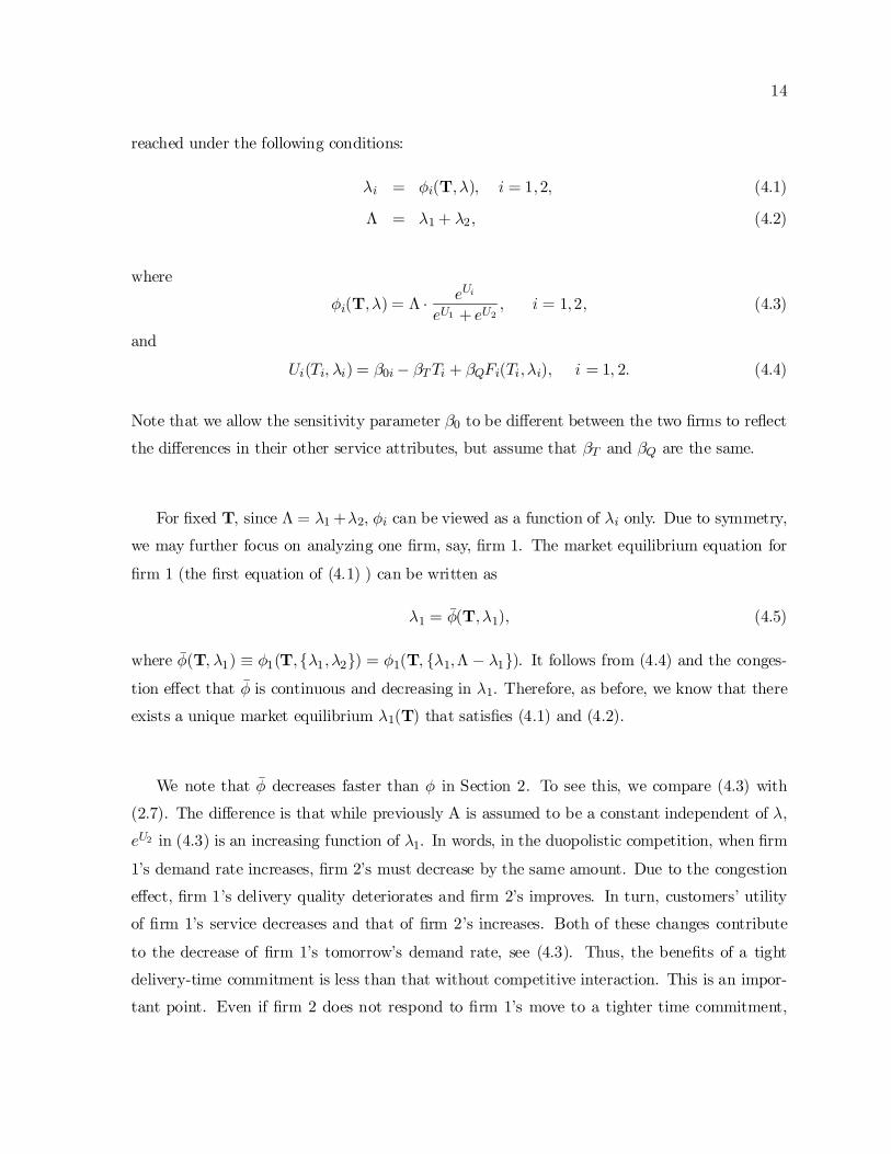
reached under the following conditions:

¸i = Ái(T;¸); i = 1;2; (4.1)

¤ = ¸1 + ¸2; (4.2)

where

Ái(T;¸) = ¤ ¢ eUieU1 + eU2

; i = 1;2; (4.3)

and

Ui(Ti; i̧) = ¯0i¡ ¯TTi + ¯QFi(Ti;¸i); i = 1; 2: (4.4)

Note that we allow the sensitivity parameter ¯0 to be di®erent between the two ¯rms to re°ect

the di®erences in their other service attributes, but assume that ¯T and ¯Q are the same.

For ¯xed T, since ¤ = ¸1 +¸2, Ái can be viewed as a function of ¸i only. Due to symmetry,

we may further focus on analyzing one ¯rm, say, ¯rm 1. The market equilibrium equation for

¯rm 1 (the ¯rst equation of (4.1) ) can be written as

¸1 = ¹Á(T;¸1); (4.5)

where ¹Á(T; ¸1) ´ Á1(T;f¸1;¸2g) = Á1(T; f¸1;¤ ¡ ¸1g). It follows from (4.4) and the conges-

tion e®ect that ¹Á is continuous and decreasing in ¸1. Therefore, as before, we know that there

exists a unique market equilibrium ¸1(T) that satis¯es (4.1) and (4.2).

We note that ¹Á decreases faster than Á in Section 2. To see this, we compare (4.3) with

(2.7). The di®erence is that while previously A is assumed to be a constant independent of ¸,

eU2 in (4.3) is an increasing function of ¸1. In words, in the duopolistic competition, when ¯rm

1's demand rate increases, ¯rm 2's must decrease by the same amount. Due to the congestion

e®ect, ¯rm 1's delivery quality deteriorates and ¯rm 2's improves. In turn, customers' utility

of ¯rm 1's service decreases and that of ¯rm 2's increases. Both of these changes contribute

to the decrease of ¯rm 1's tomorrow's demand rate, see (4.3). Thus, the bene¯ts of a tight

delivery-time commitment is less than that without competitive interaction. This is an impor-

tant point. Even if ¯rm 2 does not respond to ¯rm 1's move to a tighter time commitment,

15

¯rm 2's delivery quality will improve as a result of less congestion. This challenges the wisdom

that a drop in delivery-time will lead to a quantum leap in market share.

Next, we address the question of whether a Nash equilibrium exists in this duopolistic com-

petition. A set of time commitments is in equilibrium if, given time commitments of other ¯rms,

a ¯rm cannot increase its own market share by choosing a time commitment other than the equi-

librium time commitment. To show its existence, it su±ces to show that ¸1(T) = ¸1(fT1;T2g)is unimodal in T1 for any given T2 (i.e., ¸1(T) is quasi-concave in T1 given T2). Fix T2. Focus

on ¯rm 1 so that we may drop the subscript 1 whenever this would not cause confusion. Let¹̧(T )´ ¸1(fT; T2g). It is geometrically clear (see Figure 3) that in order to show the unimodal-

ity of ¹̧(T), it su±ces to show that for any Tc > T b > Ta,

(i) ¹Á(fTb;T2g; 0) < ¹Á(fTa;T2g; 0),

(ii) ¹Á(fTb;T2g; ¸) and ¹Á(fTa;T2g; ¸) cross at most once; and

(iii) Á(fTc;T2g;¸) and Á(fTb;T2g; ¸) do not cross before Á(fTb;T2g;¸) and Á(fTa;T2g;¸) do.

f Insert Figure 3 g

Since for ¯xed ¸, U2 is the same for ¹Á's with di®erent T1 values, and since ¹Á is strictly

increasing in U1, it su±ces to show the above properties (i){ (iii) for U1 instead of ¹Á.

Proposition 4 Nash equilibrium exists if the service processes of the two ¯rms in the duopolis-

tic competition are M=M=1 systems and the delivery time of interest is the total system time.

Proof:

1. When ¸' 0, the delivery quality is F (T; 0) = 1¡ e¡¹T (see equation 2.3), and U (T; 0) =

¯0¡¯TT +¯Q(1¡ e¡¹T ); which is the utility function of the corresponding uncongested

system. Note that U (T; 0) is not monotone in T . In fact, from the discussion in Section

3.1, we know that U (T; 0) is concave and reaches its maximum at To = 1¹ ln( ¯Q¹¯T ). We

16

also know when the delivery quality is su±ciently high, the optimal time commitment is

decreasing in the service rate. For any positive ,̧ U(T;¸) = ¯0¡¯TT+¯Q(1¡e¡(¹¡ )̧T ),

which can be viewed as the utility function of the uncongested system with an e®ective

service rate ¹̂ = ¹ ¡ ¸(< ¹). Therefore, the ¯rm's choice of time commitment must be

larger than To. So, we may restrict our discussion within the range of fT : T > Togwithout loss of rigor. Clearly, U(T; 0) is decreasing in T.

2. We show that for any T b > Ta, U (T b; ¸) ¡ U (T a;¸) is monotonely increasing in the

relevant range of ,̧ which in turn implies that U(Ta; ¸) and U (T b; ¸) cross at most once.

Since

d[U (Tb;¸)¡ U(T a; ¸)]d¸

= Tae¡(¹¡ )̧Ta ¡T be¡(¹¡ )̧Tb ;

it reduces to show that Te¡(¹¡ )̧T is decreasing in T . Di®erentiating it with respect

to T, we have @(Te¡(¹¡ )̧T )=@T = e¡(¹¡¸)T ¡ T(¹ ¡ ¸)e¡(¹¡¸)T . It is negative when

T (¹¡¸) > 1, or the delivery quality is higher than 63.2%. Therefore, we have shown that

U (Ta;¸) and U(Tb;¸) cross at most once in the range of ¸ where the delivery quality is

higher than 63.2%.

3. For any Tc > Tb > Ta(> To). Let ¸ab be an intersection of U (T a;¸) and U (T b; ¸), and

¸bc be an intersection of U(T b;¸) and U(T c; ¸). By de¯nition, we have U(Ta;¸ab) =

U (Tb;¸ab) and U(Tb;¸bc) = U (Tc;¸bc). From these two equalities, we obtain

F(Tb;¸ab)¡ F(Ta;¸ab)Tb ¡ Ta =

¯T¯Q

=F(T c; ¸bc)¡ F(Tb;¸bc)

T c¡ Tb :

We need to show that U(T c; ¸ab) < U(Tb;¸ab) and U(Ta;¸bc) < U (Tb;¸bc). The ¯rstinequality is true since

U (T c ; ¸ab) ¡ U(T b; ¸ab) = ¯Q(T c ¡ T b)[F (T c; ¸ab)¡ F (T b; ¸ab)T c ¡ T b ¡ ¯T

¯Q];

= ¯Q(T c ¡ T b)[F (T c; ¸ab)¡ F (T b; ¸ab)T c ¡ T b ¡ F (T b ; ¸ab) ¡ F (T a; ¸ab)

T b ¡ Ta ];

and F(T; ¸) is (exponentially) concave in T . Similarly, U(T a; ¸bc)< U(Tb;¸bc) because

U (T b; ¸bc)¡ U (Ta ; ¸bc) = ¯Q(T b ¡ T a)[F (T b; ¸bc)¡ F (T a; ¸bc)

T b ¡ T a ¡ F (T c; ¸bc)¡ F (T b ;¸bc)T c ¡ T b ]:

Thus, ¹̧(T ) is unimodal, and the proposition is proven.

17

For ¯rms with M=M=c service systems and the queuing time being of interest, it is easy to

show that (i) and (iii) holds: (i) is true because when ¸ ' 0, the service quality F(T; 0) = 1 (a

customer hardly needs to wait). Therefore, U(T;0) = ¯0¡¯TT, and it is obvious that U (T;0) is

decreasing in T ; (iii) holds because the waiting time distribution is also exponential and hence

concave in T. For general M=M=c case, we have not been able to prove analytically that (ii)

holds. We conjecture this on the basis of numerical examples. We prove this for the special

case of M=M=1 with queuing time.

Proposition 5 Nash equilibrium exists if the service processes of the ¯rms in the duopolistic

competition are M=M=1 systems and the delivery time of interest is the waiting time in queue.

Proof: The service quality of theM=M=1 system (in waiting time) is F(T;¸) = 1¡ ¸¹e¡(¹¡¸)T .

As before, we needs to show that @F=@¸ is an increasing function of T . Since

@F=@¸ =¡ 1¹e¡(¹¡¸)T ¡ ¸

¹Te¡(¹¡ )̧T;

where the ¯rst term is clearly increasing in T , and the second has been shown (in the proof of

the previous proposition) to be increasing in the range of (¹ ¡¸)T > 1. For ¸ in the range of

(¹¡¸)T < 1 and F(T; ¸) is high, we need to show that

@2F@¸@T

= ¹¡ 2¸+¸T(¹¡ ¸) ¸ 0;

which holds true for ¹ ¸ 2 .̧ Note, however, that for (¹ ¡ ¸)T > 1, the service quality

Q < 1¡ (¸=¹)e¡1. The service level would be lower than 1 ¡ (1=2)e¡1 ' :82, which is not

relevant in today's service environment.

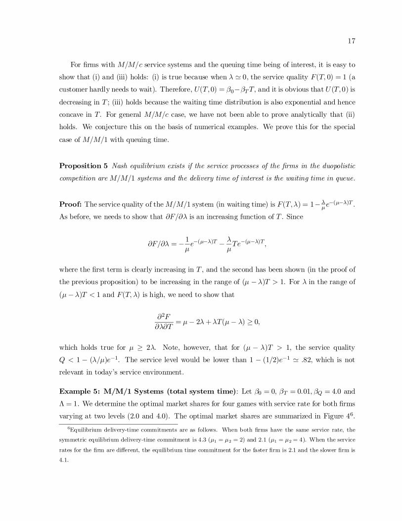
Example 5: M/M/1 Systems (total system time): Let ¯0 = 0, ¯T = 0:01; ¯Q = 4:0 and

¤ = 1. We determine the optimal market shares for four games with service rate for both ¯rms

varying at two levels (2.0 and 4.0). The optimal market shares are summarized in Figure 46.6Equilibrium delivery-time commitments are as follows. When both r̄ms have the same service rate, the

symmetric equilibrium delivery-time commitment is 4.3 (¹1 = ¹2 = 2) and 2.1 (¹1 = ¹2 = 4). When the service

rates for the ¯rm are di®erent, the equilibrium time commitment for the faster ¯rm is 2.1 and the slower ¯rm is

4.1.

18

In Figure 4, the ¯rst number in each cell is the payo® (in units of market share) to ¯rm 1 and

the second number to ¯rm 2. For instance, when both ¯rms have the same capacity of 2.0,

each ¯rm receives a payo® of 0.5. The value of ² captures the additional cost of high service

capacity. If ² is smaller than 0.01, then the game is similar to a Prisoners' Dilemma. Both

¯rms will choose a service rate of 4.0 and receive a pareto-inferior payo® of 0:5¡ ². If ² > 0:01,

then the equilibrium is (2.0, 2.0) with both ¯rms receiving 0.5. Finally, it is worth noting that

while both ¯rms will experience a lower payo® for investing in additional service capacity, the

resulting levels of delivery quality experienced by the customers will be higher.

f Insert Figure 4 g

5 Conclusion and Future Research

In this paper, we have presented a simple model for studying how a ¯rm should set its delivery-

time guarantee in managing service delivery. The model integrates the gap model of service

quality from marketing with the classical queuing models from operations. We obtain a closed-

form solution for the optimal delivery-time commitment when the ¯rm has an ample capacity.

Under congestion, we characterize the optimal delivery-time commitment with a set of condi-

tions and use it to design a computational scheme. We prove the existence of Nash equilibria

in a duopolistic game and show that the delivery-time game is similar to a Prisoners' Dilemma

when the cost of adding capacity is small.

The model allows us to study several marketing-operations interface issues. First, if there

exists multiple classes of customers which have signi¯cantly di®erent ¯T and ¯Q values, then the

delivery-time commitment for each class may be di®erent and it would be interesting to examine

how the delivery-time commitment decision is tied to the pricing in each service class. So and

Song (1998) and So (2000) consider the pricing issue in a single market segment case. Second,

if a ¯rm has service outlets in multiple locations with di®erent total demand intensity and level

of competition, it will be interesting to analyze the choice of a delivery-time commitment and

the capacity design problem for each service outlet. Finally, if the reputation of a ¯rm's service

19

quality takes time to spread through the population, it is worthwhile to see how this might

impact the choice of a delivery-time commitment (c.f., Gans, 2002).

References

[1] Anderson, R. E. `Consumer dissatisfaction: The e®ect of discon¯rmed expectancy on per-

ceived product performance,' Journal of Marketing Research 10 (February 1973): 38-44.

[2] Boulding, W.; Staelin, R.; Kalra, A.; and Zeithamal, A. `A Dynamic Process Model of Ser-

vice Quality: From Expectations to Behavioral Intentions,' Journal of Marketing Research,

1994.

[3] Carmon, Z.; Shanthikumar, G. and Carmon, T. F. `A Psychological Perspective on Service

Segmentation: The Signi¯cance of Accounting for Consumers' Perceptions of Waiting and

Service,' Management Science, 41, 1806-1815, 1995.

[4] Cooper R. B. `Queueing Theory,' Chapter 10 in Stochastic Models, Handbooks in Oper-

ations Research and Management Science, Vol. 2, (eds. Heyman D. P. and Sobel, M. J.)

North-Holland, Amsterdam,1990.

[5] Cooper, L. G., `Market-Share Models' Chapter 6 in Marketing, Handbooks in Operations

Research and Management Science, Vol. 3, (eds. J. Eliashberg and G. L. Lilien) North-

Holland, Amsterdam,1993.

[6] Gans, N. `Customer Loyalty and Supplier Quality Competition,' Management Science, 48,

202-221, 2002.

[7] Greenleaf, E. and Lehmann, D. R., `A Typology of Reasons for Substantial Delay in

Consumer Decision Making,' Journal of Consumer Research, 22 (September), 186-99, 1995.

[8] Green, L. and Kolesar, P. `On the validity and utility of queueing models of human service

systems,' Annals of Operations Research, 1987, 9:469-479.

[9] Green, L.; Lehmann, D. and Schmitt, B. `Queues, Service, and Customer Satisfaction:

A Framework for Managing Time Perceptions,' Columbia University Graduate School of

Business Working Paper, 1992.

20

[10] Hall, R. W. Queueing Methods for Services and Manufacturing, Prentice Hall, New Jersey,

1991.

[11] Katz, K. L.; Larson, B. M.; Larson, R. C. `Prescription for the waiting-in-line blues:

Entertain, enlighten, and engage,' Sloan Management Review (Winter 1991): 44-53.

[12] Kleinrock, L. Queueing Systems, Vol I:Theory. John Wiley and Sons, 1975.

[13] Larson, R. C.`Perspectives on queues: Social justice and the psychology of queuing,' Op-

erations Research 35 (Nov-Dec 1987): 895-905.

[14] Lee, H. and Cohen, M. `Equilibrium analysis of disgregate facility choice systems subject

to congestion-elastic demand,' Operations Research 33 (March-April 1985): 293-311.

[15] Lilien, G. L.; Kotler, P.; and Moorthy, K. S. Marketing Models, Prentice Hall, 1992.

[16] McFadden, D. `Econometric models for probabilistic choice among products,' Journal of

Business, 53(3):513-530, Part 2, July.

[17] Oliver, R. L. `E®ect of expectation and discon¯rmation of post-exposure product evalua-

tion:An alternative interpretation,' Journal of Applied Psychology 62 (April 1977): 480-6.

[18] Parasuraman, A.; Zeithaml, V. A.; Berry, L. `A conceptual model of service quality and

implications for future research,' Journal of Marketing 64(Spring 1985): 12-40.

[19] Rothkopf, M. and Reck, P. `Perspectives on queues,: Combining queues is not always

bene¯cial,' Operations Research, 35:906-909, 1987.

[20] So, R. and Song, J. S. `Price, Delivery Time Guarantees and Capacity Selection,' European

Journal of Operational Research, 111(1), 28-49 (1998).

[21] So, R. `Price and Time Competition for Service Delivery,' Manufacturing and Services

Operations Management, 2(4), 392-409 (2000).

[22] Tse, D. K. and Wilton, P. C. `Models of consumer satisfaction formation: An extension,"

Journals of Marketing Research, 25:203-212, 1988.

[23] Zeithaml, V., B. Berry and A. Parasuraman `The nature and determinants of customer

expectations of service,' Marketing Science Institute, Cambridge MA, Working Paper,

1991.

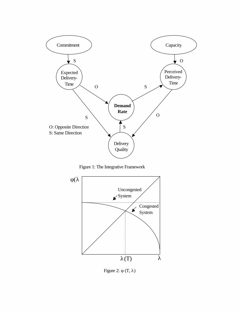
Figure 1: The Integrative Framework

Figure 2: φ (T, λ)

Commitment Capacity

Expected Delivery-

Time

Perceived Delivery-

Time

Demand Rate

Delivery Quality

S O

O

O

S

S

S

O: Opposite Direction S: Same Direction

Uncongested System

Congested System

φ(λ)

λ(T) λ

Figure 3: Proof of Existence of Nash Equilibrium

Figure 4: The Duopolistic Game

Firm 2’s Service Rate (µ2)

Firm 1’s Service Rate (µ1)

2.0

2.0

4.0

4.0

0.5, 0.5 0.49, 0.51 - ε

0.51 – ε, 0.49 0.5 – ε, 0.5 − ε

λab λbc

Ta

Tb

Tc

Λ

Λ