conditional expectation
TRANSCRIPT

Conditional Expectation
Andreas Klappenecker
Texas A&M University
© 2018 by Andreas Klappenecker. All rights reserved.
1 / 63

Conditional Expectation
We are going to define the conditional expectation of a randomvariable given
1 an event,
2 another random variable,
3 a σ-algebra.
Conditional expectations can be convenient in some computations.
2 / 63

Conditional Expectation given an Event
DefinitionThe conditional expectation of a discrete random variable Xgiven an event A is denoted as ErX | As and is defined by
ErX | As “ÿ
x
x PrrX “ x | As.
It follows that
ErX | As “ÿ
x
x PrrX “ x | As “ÿ
x
xPrrX “ x and As
PrrAs.
3 / 63
Example
Problem
Suppose that X and Y are discrete random variables with values in t1, 2u s.t.
PrrX “ 1,Y “ 1s “ 12, PrrX “ 1,Y “ 2s “ 1
10,
PrrX “ 2,Y “ 1s “ 110, PrrX “ 2,Y “ 2s “ 3
10.
Calculate ErX | Y “ 1s.
By definition
ErX | Y “ 1s “ 1 PrrX “ 1 | Y “ 1s ` 2 PrrX “ 2 | Y “ 1s.
“ 1PrrX “ 1,Y “ 1s
PrrY “ 1s` 2
PrrX “ 2,Y “ 1s
PrrY “ 1s.
4 / 63

Example
Problem
Suppose that X and Y are discrete random variables with values in t1, 2u s.t.
PrrX “ 1,Y “ 1s “ 12, PrrX “ 1,Y “ 2s “ 1
10,
PrrX “ 2,Y “ 1s “ 110, PrrX “ 2,Y “ 2s “ 3
10.
We have PrrY “ 1s “ PrrX “ 1,Y “ 1s ` PrrX “ 2,Y “ 1s “ 12` 1
10“ 3
5.
ErX | Y “ 1s “ 1PrrX “ 1,Y “ 1s
PrrY “ 1s` 2
PrrX “ 2,Y “ 1s
PrrY “ 1s
“ 112
35` 2
110
35“
5
6` 2
1
6“
7
6
5 / 63
Conditional Expectation
Interpretation
Let F “ 2Ω with Ω finite. For a random variable X and an event A,we can interpret ErX | As as the average of X pωq over all ω P A.
Indeed, we have
ErX |As “ÿ
x
x PrrX “ x | As “ÿ
x
xPr rX “ x and As
PrrAs
“ÿ
ωPA
X pωqPrrωs
PrrAs.
Caveat
This interpretation does not work for all random variables, but it gives a better understandingof the meaning of ErX | As.
6 / 63

Conditional Expectation
PropositionWe have
ErX | As “ErX IAs
PrrAs.
Proof.
As we have seen,
ErX |As “ÿ
x
xPr rX “ x and As
PrrAs“
1
PrrAs
ÿ
x
xPr rX “ x and As.
We can rewrite the latter expression in the form
ErX |As “ErX IAs
PrrAs.
7 / 63

Definition for General Random Variables
Definition
The conditional expectation ErX | As of an arbitrary randomvariable X given an event A is defined by
ErX |As “
$
&
%
ErX IAs
PrrAsif PrrAs ą 0,
0 otherwise.
8 / 63
Properties
9 / 63

Linearity
Proposition
If a and b are real numbers and X and Y are random variables, then
EraX ` bY | As “ aErX | As ` bErY | As.
Proof.
EraX ` bY | As “ErpaX ` bY q IAs
PrrAs
“ aErX IAs
PrrAs` b
ErY IAs
PrrAs
“ aErX | As ` bErY | As.
10 / 63

Independence
Proposition
If X and Y are independent discrete random variables, then
ErY | X “ xs “ ErY s.
Proof.By definition,
ErY | X “ xs “ÿ
y
y PrrY “ y | X “ xs
“ÿ
y
y PrrY “ y s “ ErY s.
11 / 63

Important Application
12 / 63
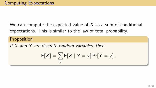
Computing Expectations
We can compute the expected value of X as a sum of conditionalexpectations. This is similar to the law of total probability.
Proposition
If X and Y are discrete random variables, then
ErX s “ÿ
y
ErX | Y “ y sPrrY “ y s.
13 / 63
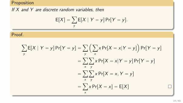
Proposition
If X and Y are discrete random variables, then
ErX s “ÿ
y
ErX | Y “ y sPrrY “ y s.
Proof.
ÿ
y
ErX | Y “ y sPrrY “ y s “ÿ
y
´
ÿ
x
x PrrX “ x |Y “ y s¯
PrrY “ y s
“ÿ
x
ÿ
y
x PrrX “ x |Y “ y sPrrY “ y s
“ÿ
x
ÿ
y
x PrrX “ x ,Y “ y s
“ÿ
x
x PrrX “ xs “ ErX s
14 / 63

Why We Need More than One Type ofConditional Expectation
15 / 63
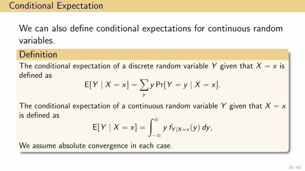
Conditional Expectation
We can also define conditional expectations for continuous randomvariables.
DefinitionThe conditional expectation of a discrete random variable Y given that X “ x isdefined as
ErY | X “ xs “ÿ
y
y PrrY “ y | X “ xs.
The conditional expectation of a continuous random variable Y given that X “ xis defined as
ErY | X “ xs “
ż 8
´8
y fY |X“xpyq dy ,
We assume absolute convergence in each case.
16 / 63

Motivating Example
ProblemA stick of length one is broken at a random point, uniformlydistributed over the stick. The remaining piece is broken oncemore.
Find the expected value of the piece that now remains.
17 / 63
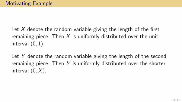
Motivating Example
Let X denote the random variable giving the length of the firstremaining piece. Then X is uniformly distributed over the unitinterval p0, 1q.
Let Y denote the random variable giving the length of the secondremaining piece. Then Y is uniformly distributed over the shorterinterval p0,X q.
18 / 63

Motivating Example: Interpretation
Given that X “ x , the random variable Y is uniformly distributedover the interval p0, xq. In other words,
Y | X “ x
has the density function
fY |X“xpyq “1
x
for all y in p0, xq.
19 / 63

Motivating Example: Expectation
For a random variable Z that is uniformly distributed on the interval pa, bq, wehave
ErZ s “
ż b
a
x1
b ´ adx “
1
b ´ a
1
2x2ˇ
ˇ
ˇ
ˇ
b
a
“b2 ´ a2
2pb ´ aq“
b ` a
2.
Example
Since the random variable X is uniformly distributed over the interval p0, 1q, wehave
ErX s “1` 0
2“
1
2.
20 / 63
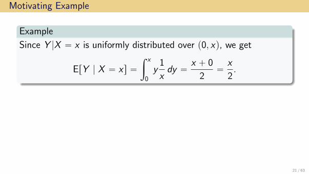
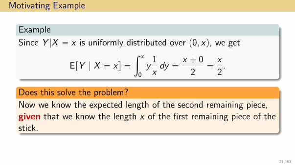
Motivating Example
Example
Since Y |X “ x is uniformly distributed over p0, xq, we get
ErY | X “ xs “
ż x
0
y1
xdy “
x ` 0
2“
x
2.
Does this solve the problem?
Now we know the expected length of the second remaining piece,given that we know the length x of the first remaining piece of thestick.
21 / 63
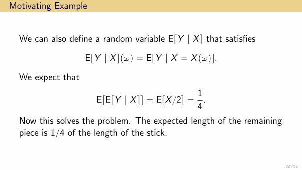
Motivating Example
We can also define a random variable ErY | X s that satisfies
ErY | X spωq “ ErY | X “ X pωqs.
We expect that
ErErY | X ss “ ErX 2s “1
4.
Now this solves the problem. The expected length of the remainingpiece is 1/4 of the length of the stick.
22 / 63

Conditional Expectation given a RandomVariable
23 / 63

Motivation
Question
How should we think about ErX | Y s?
Answer
Suppose that Y is a discrete random variable. If we observe one of the values yof Y , then the conditional expectation should be given by
ErX | Y “ y s.
If we do not know the value y of Y , then we need to contend ourselves withthe possible expectations
ErX | Y “ y1s, ErX | Y “ y2s, ErX | Y “ y2s, . . .
So ErX | Y s should be a σpY q-measurable random variable itself.
24 / 63

Definition
DefinitionLet X and Y be two discrete random variables.
The conditional expectation ErX | Y s of X given Y is therandom variable defined by
ErX | Y spωq “ ErX | Y “ Y pωqs.
Caveat
Sometimes ErX | Y s is defined differently as a BpRq-measurable functiony ÞÑ ErX | Y “ y s. We prefer to think about ErX | Y s as a function Ω Ñ R.The two definitions are obviously not equivalent. Our choice generalizes nicely.
25 / 63

A Pair of Fair Coin Flips
Example
Suppose that X and Y are random variables describing independentfair coin flips with values 0 and 1. Then the sample space ofpX ,Y q is given by
Ω “ tp0, 0q, p0, 1q, p1, 0q, p1, 1qu.
Let Z denote the random variable Z “ X ` Y . Then we have
Z p0, 0q “ 0, Z p0, 1q “ 1, Z p1, 0q “ 1, Z p1, 1q “ 2.
26 / 63

A Pair of Fair Coin Flips
Example (Continued.)
Suppose that we want to know ErZ | X s. We calculate
ErZ | X “ 0s “ 0 ¨1
2` 1 ¨
1
2“
1
2,
ErZ | X “ 1s “ 1 ¨1
2` 2 ¨
1
2“
3
2.
ThenErZ | X sp0, 0q “ 1
2 , ErZ | X sp0, 1q “ 12 ,
ErZ | X sp1, 0q “ 32 , ErZ | X sp1, 1q “ 3
2 .
27 / 63
A Pair of Fair Coin Flips
Example (Continued.)
Suppose that we now want to know ErZ | Y s. We calculate
ErZ | Y “ 0s “ 0 ¨1
2` 1 ¨
1
2“
1
2,
ErZ | Y “ 1s “ 1 ¨1
2` 2 ¨
1
2“
3
2.
ThenErZ | Y sp0, 0q “ 1
2 , ErZ | Y sp0, 1q “ 32 ,
ErZ | Y sp1, 0q “ 12 , ErZ | Y sp1, 1q “ 3
2 .
28 / 63

A Pair of Fair Coin Flips
Example (Continued.)
Suppose that we now want to know ErX | Z s. We calculate
ErX | Z “ 0s “ 0
ErX | Z “ 1s “ 0 ¨1
2` 1 ¨
1
2“
1
2,
ErX | Z “ 2s “ 1
ThenErX | Z sp0, 0q “ 0, ErX | Z sp0, 1q “ 1
2 ,
ErX | Z sp1, 0q “ 12 , ErX | Z sp1, 1q “ 1.
29 / 63

Properties of the Conditional Expectation
30 / 63

Functions
Proposition
If X is a function of Y , then ErX | Y s “ X .
Proof.
Suppose that X “ f pY q. Then
ErX | Y spωq “ ErX | Y “ Y pωqs
“ Erf pY pωqq | Y “ Y pωqs
“ f pY pωqq “ X pωq.
31 / 63
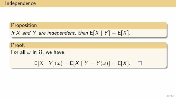
Independence
Proposition
If X and Y are independent, then ErX | Y s “ ErX s.
Proof.For all ω in Ω, we have
ErX | Y spωq “ ErX | Y “ Y pωqs “ ErX s.
32 / 63

Linearity
Proposition
If a and b are real numbers and X ,Y , and Z discrete randomvariables, then
EraX ` bY | Z s “ aErX | Z s ` bErY | Z s.
33 / 63

A Pair of Fair Coin Flips
Example
Suppose that X and Y are independent random variables describingfair coin flips with values 0 and 1. Let Z “ X ` Y . We determinedErZ |X s, but it was a bit cumbersome. Here is an easier way:
ErZ | X s “ ErX ` Y | X s by definition
“ ErX | X s ` ErY | X s by linearity
“ X ` ErY s by function and by independence
“ X `1
2.
34 / 63

Law of the Iterated Expectation
Proposition
ErErX | Y ss “ ErX s.
Proof.
ErErX | Y ss “ÿ
y
ErErX | Y s|Y “ y sPrrY “ y s
“ÿ
y
ErX | Y “ y sPrrY “ y s
“ ErX s
35 / 63

Applications
36 / 63

Wald’s Theorem
TheoremSuppose that X1,X2, . . . are independent random variables, all withthe same mean. Suppose that N is a nonnegative, integer-valuedrandom variable that is independent of the Xi ’s. If ErX1s ă 8 andErNs ă 8, then
E
«
Nÿ
k“1
Xi
ff
“ ErNsErX1s.
37 / 63

Proof.By double expectation, we have
E
«
Nÿ
k“1
Xi
ff
“ E
«
E
«
Nÿ
k“1
Xi
ˇ
ˇ
ˇ
ˇ
N
ffff
“
8ÿ
n“1
E
«
Nÿ
k“1
Xi
ˇ
ˇ
ˇ
ˇ
N “ n
ff
PrrN “ ns
“
8ÿ
n“1
E
«
nÿ
k“1
Xi
ˇ
ˇ
ˇ
ˇ
N “ n
ff
PrrN “ ns
38 / 63

Proof. (Continued)
E
«
Nÿ
k“1
Xi
ff
“
8ÿ
n“1
E
«
nÿ
k“1
Xi
ˇ
ˇ
ˇ
ˇ
N “ n
ff
PrrN “ ns
“
8ÿ
n“1
E
«
nÿ
k“1
Xi
ff
PrrN “ ns
“
8ÿ
n“1
nE rX1sPrrN “ ns
“ ErX1s
8ÿ
n“1
n PrrN “ ns “ ErX1sErNs. 2
39 / 63

Dice
Example
Suppose that we roll a navy die. The face value N of the die rangesfrom 1 to 6. Depending on the face value of the navy die, we roll Nivory dice and sum their values.
On average, what is the resulting value of the sum face values ofthe N ivory dice?
40 / 63
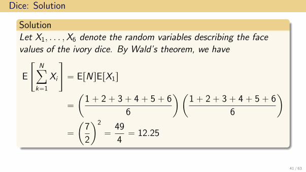
Dice: Solution
SolutionLet X1, . . . ,X6 denote the random variables describing the facevalues of the ivory dice. By Wald’s theorem, we have
E
«
Nÿ
k“1
Xi
ff
“ ErNsErX1s
“
ˆ
1` 2` 3` 4` 5` 6
6
˙ˆ
1` 2` 3` 4` 5` 6
6
˙
“
ˆ
7
2
˙2
“49
4“ 12.25
41 / 63

Conditional Expectation Given a σ-Algebra
42 / 63

Motivation
Suppose that a sample space Ω is partitioned into measurable sets
B1,B2, . . . ,Bn.
We know know the expectation of a random variable X given thatone of the events Bk will happen, but we do not know which one.
We want to form a conditional expectation ErX | Gs withG “ σpB1,B2, . . . ,Bnq such that
ErX | Gspωq “ ErX | Bks “ErX IBk
s
PrrBks
for ω P Bk . Then ErErX | Gs s “ ErX s.43 / 63

Conditional Expectation
DefinitionLet F be a σ-algebra with sub-σ-algebra G. A random variable Y iscalled a conditional expectation of X given G, writtenY “ ErX | Gs if and only if
1 Y is G-measurable
2 ErY IG s “ ErX IG s for all G P G.
44 / 63

Single Event
Example
Let A and B be events with 0 ă PrrAs ă 1. If we define G “ σpBq,then G “ tH,B ,Bc ,Ωu. Then
ErX | Gs “ ErX IBs
PrrBsIB `
ErX IBc s
PrrBcsIBc .
Indeed, the right-hand side is clearly G-measurable. We have
ErErX | GsIB s “ ErX IBs
andErErX | GsIBc s “ ErX IBc s.
45 / 63
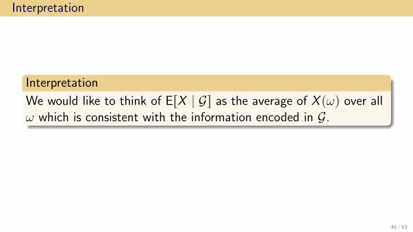
Interpretation
Interpretation
We would like to think of ErX | Gs as the average of X pωq over allω which is consistent with the information encoded in G.
46 / 63

σ-Algebra Generated by a Random Variable
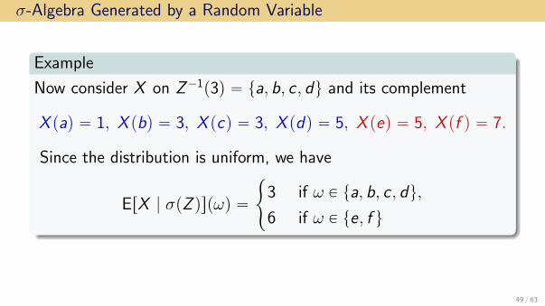
Example
Suppose that pΩ,F ,Prq is a probability space withΩ “ ta, b, c , d , e, f u, F “ 2Ω, and Pr uniform. Define a randomvariable X by
X paq “ 1, X pbq “ 3, X pcq “ 3, X pdq “ 5, X peq “ 5, X pf q “ 7.
Suppose that another random variable Z is given by
Z paq “ 3, Z pbq “ 3, Z pcq “ 3, Z pdq “ 3, Z peq “ 2, Z pf q “ 2.
We want to determine ErX | Gs with G “ σpZ q.
47 / 63

σ-Algebra Generated by a Random Variable
Example
Since
Z paq “ 3, Z pbq “ 3, Z pcq “ 3, Z pdq “ 3, Z peq “ 2, Z pf q “ 2,
the σ-algebra σpZ q is generated by the event Z´1p3q and itscomplement
Z´1p3q “ ta, b, c , du and Z´1
p2q “ te, f u.
48 / 63
σ-Algebra Generated by a Random Variable
Example
Now consider X on Z´1p3q “ ta, b, c , du and its complement
X paq “ 1, X pbq “ 3, X pcq “ 3, X pdq “ 5, X peq “ 5, X pf q “ 7.
Since the distribution is uniform, we have
ErX | σpZ qspωq “
#
3 if ω P ta, b, c , du,
6 if ω P te, f u
49 / 63
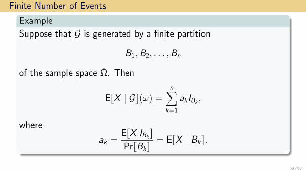
Finite Number of Events
Example
Suppose that G is generated by a finite partition
B1,B2, . . . ,Bn
of the sample space Ω. Then
ErX | Gspωq “nÿ
k“1
ak IBk,
where
ak “ErX IBk
s
PrrBks“ ErX | Bks.
50 / 63

Finite Number of Events
Example (Continued.)
If
ErX | Gs “nÿ
k“1
ErX IBks
PrrBksIBk,
then it is certainly G-measurable and
ErErX | Gs sIBks “ ErX IBk
s.
Therefore,
ErErX | Gs s “nÿ
k“1
ErX IBks “ ErX IΩs “ ErX s.
51 / 63

Conditional Expectation: Main Questions
DefinitionLet F be a σ-algebra with sub-σ-algebra G. A random variable Y iscalled a conditional expectation of X given G, writtenY “ ErX | Gs if and only if
1 Y is G-measurable
2 ErY IG s “ ErX IG s for all G P G.
Questions1 Is the conditional expectation unique?
2 Does conditional expectation always exist?
52 / 63
Uniqueness
Suppose that Y and Y 1 are G-measurable random variables suchthat
ErY IG s “ ErX IG s “ ErY 1 IG s
holds for all G P G. Then G “ tY ą Y 1u is an event in G. We have
0 “ ErY IAs ´ ErY 1 IAs “ ErpY ´ Y 1qIAs.
Since pY ´ Y 1qIA ě 0, we have PrrAs “ 0.
We can conclude that Y ď Y 1 almost surely (meaning withprobability 1). Similarly, Y 1 ď Y almost surely.
So Y 1 “ Y almost surely.53 / 63

Existence (Sketch for those who know integration on measures)
Let X` “ maxtX , 0u and X´ “ X` ´ X . We can define two finitemeasures on pΩ,Fq by
Q˘pAq :“ ErX˘ IAs
for all A P F .
If A satisfies PrrAs “ 0, then Q˘pAq “ 0.
Therefore, it follows from the Radon-Nikodym theorem that thereexist densities Y ˘ such that
Q˘pAq “
ż
A
Y ˘d Pr “ ErY ˘ IAs.
Now define the conditional expectation by Y “ Y ` ´ Y ´.54 / 63

Linearity
Proposition
EraX ` bY | Gs “ aErX | Gs ` bErY | Gs.
Proof.The right-hand side is G-measurable by definition, hence, for G P G
ErIG paErX | Gs ` bErY | Gsqs “ aErIGErX | Gss ` bErIGErY | Gss“ aErIGX s ` bErIGY s
“ ErIG paX ` bY qs.
55 / 63

MonotonicityProposition
If X ě Y almost surely, then
ErX | Gs ě ErY | Gs.
Proof.
Let A denote the event tErX | Gs ă ErY | Gsu P G.Since we have X ě Y , we get
ErIApX ´ Y qs ě 0.
Therefore, PrrAs “ 0.
For this proof, make sure that you understand what the event A encodes.56 / 63

Products
Proposition
If Er|XY |s ă 8 and Y is G-measurable, then
ErXY | Gs “ YErX | Gs and ErY | Gs “ ErY | Y s “ Y .
The proof is a bit more involved.
57 / 63
Tower Property
Proposition
Let G Ď F Ď A be σ-algebras. Let X be an A-measurable random variable.Then
ErErX | Fs | Gs “ ErErX | Gs | Fs “ ErX | Gs.
Proof.
The second equality follows from the product property with X “ 1 andY “ ErX | Gs, since Y is F -measurable.
If A P G, then A P F and
ErIA ErErX | Fs | Gss “ ErIAErX | Fss“ ErIA X s
“ ErIA ErX | Gss.
58 / 63

Triangle Inequality
Proposition
Er|X | | Gs ě |ErX | Gs|
59 / 63

Independence
Proposition
If σpX q and G are independent σ-algebras, so
PrrAX Bs “ PrrAsPrrBs
for all A P σpX q and B P G, then
ErX | Gs “ ErX s.
60 / 63

Lack of Information
Proposition
If PrrAs P t0, 1u for all A P G, then
ErX | Gs “ ErX s.
61 / 63

Best Prediction
The conditional expectation ErX | Gs is supposed to be the “best”prediction one can make about X if we only have the informationcontained in σ-algebra G.
Extremal Case 1
If σpX q Ď G, thenErX | Gs “ X .
Extremal Case 2
If σpX q and G are independent, then
ErX | Gs “ ErX s.
62 / 63

Best Prediction
Proposition
Let G Ď A be σ-algebras. Let X be an A-measurable randomvariable with ErX 2s ă 8. Then for any G-measurable randomvariable Y with ErY 2s ă 8, we have
ErpX ´ Y q2s ě ErpX ´ ErX | Gsq2s
with equality if and only if Y “ ErX | Gs.
63 / 63