sentinels of climate change: coastal indicators of

1

Sentinels of climate change: coastal indicators of wildlife and ecosystem change in Long Island Sound

Final report

September, 2014

Chris Field1 and Chris Elphick1,*,

With key contributions from co-investigators: Maureen Correll2, Min Huang3, and Brian Olsen2

1 Department of Ecology and Evolutionary Biology and Center for Conservation and Biodiversity, University of Connecticut, 75 North Eagleville Road, Storrs, CT 06268

2 School of Biology & Ecology, Climate Change Institute, University of Maine, Orono,

Maine 04469

3 CT Department of Energy and Environmental Protection, Migratory Game Bird Program, 391 Route 32, North Franklin, CT 06254

*Please direct correspondence to: [email protected]

Project funded by Connecticut Department of Energy and Environmental Protection/Long Island Sound Study

Summary: We investigated potential indicators of climate change effects on key wildlife and ecosystem resources in coastal Long Island Sound (LIS). Our focus was on biological indicators with high potential to show climate responses, available historical data, ease of cost-effective future data collection, and the ability to inform real-world management decisions. For wildlife measures with long enough time series, we investigated whether variation was explained by a set of core parameters: measures of temperature, precipitation, and sea level. We found that beach-nesting and colonial waterbirds, which represent some of the longest time series for wildlife in LIS, are not strongly influenced by the core parameters. In contrast, several saltmarsh bird and plant measures are strong indicators of sea level and tidal flooding. Additionally, we conducted pilot investigations and collected baseline data for other potential indicators in an attempt to address topics that lacked a historical record, in particular rates of ecosystem change in areas thought to be experiencing marine transgression. Overall, our results suggest that (1) several components of saltmarsh ecosystems are already being affected by increased coastal flooding and (2) coastal forest ecosystems are potentially resilient to change in the face of increased coastal flooding. This temporal mismatch in responses to coastal flooding will likely create challenges for management aimed at saltmarsh conservation in LIS. Additional research and monitoring is needed to understand rates of marine transgression and the factors influencing them.

2

Key recommendations: We recommend the following steps to advance monitoring biological responses to climate change along the Long Island Sound coast. Items on this list are divided into those that are of top priority (i.e., essential to tracking climate-related change) and those that are of high priority (i.e., would enhance our understanding and have good potential to improve sentinel monitoring). Lower priority recommendations can be found within the body of the report. Top priority action items:

Conduct regular monitoring of specialist saltmarsh bird (clapper rail, willet,

saltmarsh sparrow, seaside sparrow) abundance and nest success at existing

georeferenced points and using protocols now in use throughout the Northeast and

Mid-Atlantic states. Optimal survey frequency is under investigation and annual

surveys might not be necessary; until those results are available, planning for

surveys at least every 2-3 years would be conservative.

Conduct regular resurveys of the coastal margin transects created to quantify

baseline conditions during this study. Expanding this baseline survey beyond

forest habitats would broaden the inferences that can be made about marine

transgression. With only one year of data it is impossible to estimate the optimal

frequency for resurveys, but every 5-10 years is likely suitable. More frequent

surveys in the near term (e.g., annual for 3-5 years) would allow formal

investigation of optimal timing.

Conduct regular resurveys of tidal marsh vegetation at existing georeferenced

sites. Permanently marked points, newly surveyed in this study, should be visited

every 2 years to ensure that rapid change is detected and the larger, pre-existing,

set of randomly located plots should be visited every 5-10 years to ensure a

representative sample and continuation of the longer time series.

Deploy a network of “PlantCam” photo stations to quantify phenology of coastal

vegetation change. Ideally, this network should be developed such that it

simultaneously gathers data on other potential indicators of changing marsh

conditions. Siting photo stations in a manner coincident with other tidal marsh

monitoring work is also advised.

High priority action items:

Expand tree core sampling of oaks to describe spatial variation in the resilience of

coastal forests to marsh encroachment and climate-related growth patterns.

Compile historic data sets describing tidal marsh vegetation and organize them in

a consistent format. During our work we identified several such data sets, and

others have been working to make this information more accessible. Analyzing

that information was beyond the scope of our study and the wide range of

different methods used made it unclear how fruitful further analysis would prove.

Given the magnitude of vegetation change detected in our study, and uncertainty

over the magnitude and nature of longer-term (multi-decadal) vegetation change,

however, a focused project to systematically complete this task would be

valuable.

3

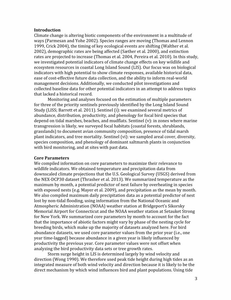
Introduction Climate change is altering biotic components of the environment in a multitude of ways (Parmesan and Yohe 2002). Species ranges are moving (Thomas and Lennon 1999, Crick 2004), the timing of key ecological events are shifting (Walther et al. 2002), demographic rates are being affected (Sæther et al. 2000), and extinction rates are projected to increase (Thomas et al. 2004, Pereira et al. 2010). In this study, we investigated potential indicators of climate change effects on key wildlife and ecosystem resources in coastal Long Island Sound (LIS). Our focus was on biological indicators with high potential to show climate responses, available historical data, ease of cost-effective future data collection, and the ability to inform real-world management decisions. Additionally, we conducted pilot investigations and collected baseline data for other potential indicators in an attempt to address topics that lacked a historical record.

Monitoring and analyses focused on the estimation of multiple parameters for three of the priority sentinels previously identified by the Long Island Sound Study (LISS; Barrett et al. 2011). Sentinel (i): we examined several metrics of abundance, distribution, productivity, and phenology for focal bird species that depend on tidal marshes, beaches, and mudflats. Sentinel (v): in zones where marine transgression is likely, we surveyed focal habitats (coastal forests, shrublands, grasslands) to document avian community composition, presence of tidal marsh plant indicators, and tree mortality. Sentinel (vi): we sampled areal cover, diversity, species composition, and phenology of dominant saltmarsh plants in conjunction with bird monitoring, and at sites with past data. Core Parameters We compiled information on core parameters to maximize their relevance to wildlife indicators. We obtained temperature and precipitation data from downscaled climate projections that the U.S. Geological Survey (USGS) derived from the NEX-DCP30 dataset (Thrasher et al. 2013). We summarized temperature as the maximum by month, a potential predictor of nest failure by overheating in species with exposed nests (e.g. Mayer et al. 2009), and precipitation as the mean by month. We also compiled maximum daily precipitation data as a potential predictor of nest lost by non-tidal flooding, using information from the National Oceanic and Atmospheric Administration (NOAA) weather station at Bridgeport’s Sikorsky Memorial Airport for Connecticut and the NOAA weather station at Setauket Strong for New York. We summarized core parameters by month to account for the fact that the importance of abiotic factors might vary by phase of the nesting cycle for breeding birds, which make up the majority of datasets analyzed here. For bird abundance datasets, we used core parameter values from the prior year (i.e., one year time-lagged) because abundance in a given year is likely influenced by productivity the previous year. Core parameter values were not offset when analyzing the bird productivity data sets or tree growth rates.

Storm surge height in LIS is determined largely by wind velocity and direction (Wong 1990). We therefore used peak tide height during high tides as an integrated measure of both wind velocity and direction because it is likely to be the direct mechanism by which wind influences bird and plant populations. Using tide

4

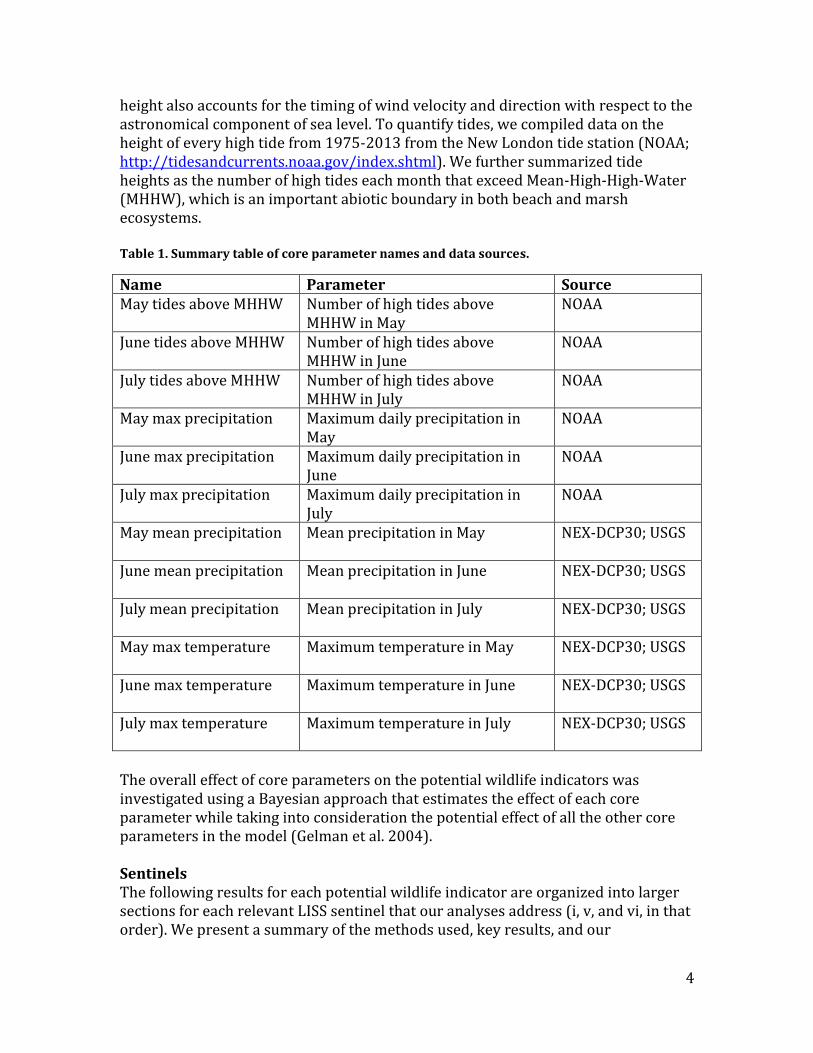
height also accounts for the timing of wind velocity and direction with respect to the astronomical component of sea level. To quantify tides, we compiled data on the height of every high tide from 1975-2013 from the New London tide station (NOAA; http://tidesandcurrents.noaa.gov/index.shtml). We further summarized tide heights as the number of high tides each month that exceed Mean-High-High-Water (MHHW), which is an important abiotic boundary in both beach and marsh ecosystems. Table 1. Summary table of core parameter names and data sources.

Name Parameter Source May tides above MHHW Number of high tides above

MHHW in May NOAA

June tides above MHHW Number of high tides above MHHW in June

NOAA

July tides above MHHW Number of high tides above MHHW in July

NOAA

May max precipitation Maximum daily precipitation in May

NOAA

June max precipitation Maximum daily precipitation in June

NOAA

July max precipitation Maximum daily precipitation in July

NOAA

May mean precipitation Mean precipitation in May

NEX-DCP30; USGS

June mean precipitation Mean precipitation in June

NEX-DCP30; USGS

July mean precipitation Mean precipitation in July

NEX-DCP30; USGS

May max temperature Maximum temperature in May

NEX-DCP30; USGS

June max temperature Maximum temperature in June

NEX-DCP30; USGS

July max temperature Maximum temperature in July

NEX-DCP30; USGS

The overall effect of core parameters on the potential wildlife indicators was investigated using a Bayesian approach that estimates the effect of each core parameter while taking into consideration the potential effect of all the other core parameters in the model (Gelman et al. 2004). Sentinels The following results for each potential wildlife indicator are organized into larger sections for each relevant LISS sentinel that our analyses address (i, v, and vi, in that order). We present a summary of the methods used, key results, and our

http://tidesandcurrents.noaa.gov/index.shtml

5

recommendations on the potential of each indicator to provide information on the core parameters and important trends in LIS ecosystems. LISS sentinel (i): Distribution, abundance, and species composition of marsh birds, colonial nesting birds, shorebirds, waterfowl. Specialist saltmarsh bird abundance Methods – In May-August of 2013, we conducted surveys of specialist saltmarsh bird abundance and habitat at 141 locations (91 in Connecticut; 50 in New York) across LIS. These surveys contributed to baseline monitoring, initiated in 2011, of the distribution, abundance, and species composition of saltmarsh birds and plants from Virginia to Maine. In 2014, surveys were repeated to further build the baseline database. Survey locations were selected for the Saltmarsh Habitat and Avian Research Program (SHARP; www.tidalmarshbirds.org) using a spatially balanced generalized random tessellation stratified (GRTS) design (see 40 km Atlantic Flyway Hexagon Grid; http://www.tidalmarshbirds.net/?page_id=1595) that ensures that the resulting data are representative of Connecticut, New York, or Long Island Sound, depending on the desired scale of inference. Using this sampling scheme, surveys can be scaled back for streamlined monitoring without losing representativeness. The survey protocol, which includes both passive sampling and a callback period for secretive marsh birds, is described in the SHARP Callback Survey Protocol at http://www.tidalmarshbirds.net/?page_id=1595.

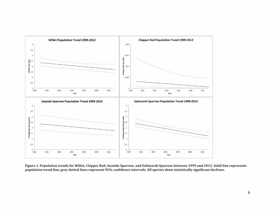
We compared surveys from 2011-2014 to historical bird surveys conducted within Connecticut by UConn (2002 – 2008, n = 110 points) and the Maine Department of Inland Fisheries and Wildlife (1999-2000, n=155 points) to quantify population trends at sites occupied by our focal specialist species: Clapper Rail, Willet, Saltmarsh Sparrow and Seaside Sparrow. The data did not contain enough observations of American Black Ducks to support analyses. We conducted analyses using generalized mixed effects models that account for point-level, hexagon-level, and year effects. Results – Our analysis shows that all focal species are declining (Figure 1). Saltmarsh Sparrows have the steepest decline, losing an average of 1.15 birds per 50-m radius point over the time span explored. Seaside Sparrows and Willets show nearly identical declines, respectively losing 0.62 and 0.63 birds per point. Clapper Rail numbers were modeled differently and are not directly comparable to the sparrow and Willet models, however, they also show a statistically significant decline. Tracking specialist saltmarsh birds as a composite group was not necessary because all species that were analyzed are declining, so the group trend will also indicate an overall decline.

http://www.tidalmarshbirds.org/

http://www.tidalmarshbirds.net/?page_id=1595


6

Figure 1. Population trends for Willet, Clapper Rail, Seaside Sparrow, and Saltmarsh Sparrow between 1999 and 2012. Solid line represents population trend line; grey dotted lines represent 95% confidence intervals. All species show statistically significant declines.

7

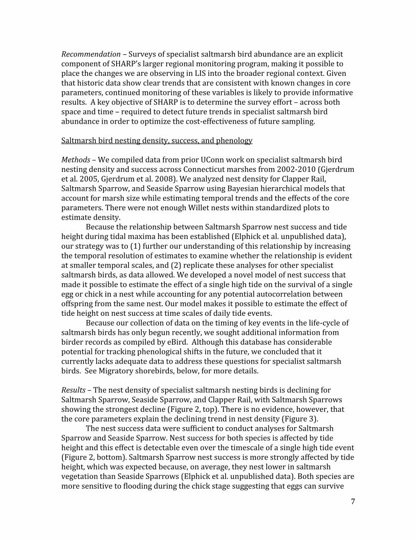
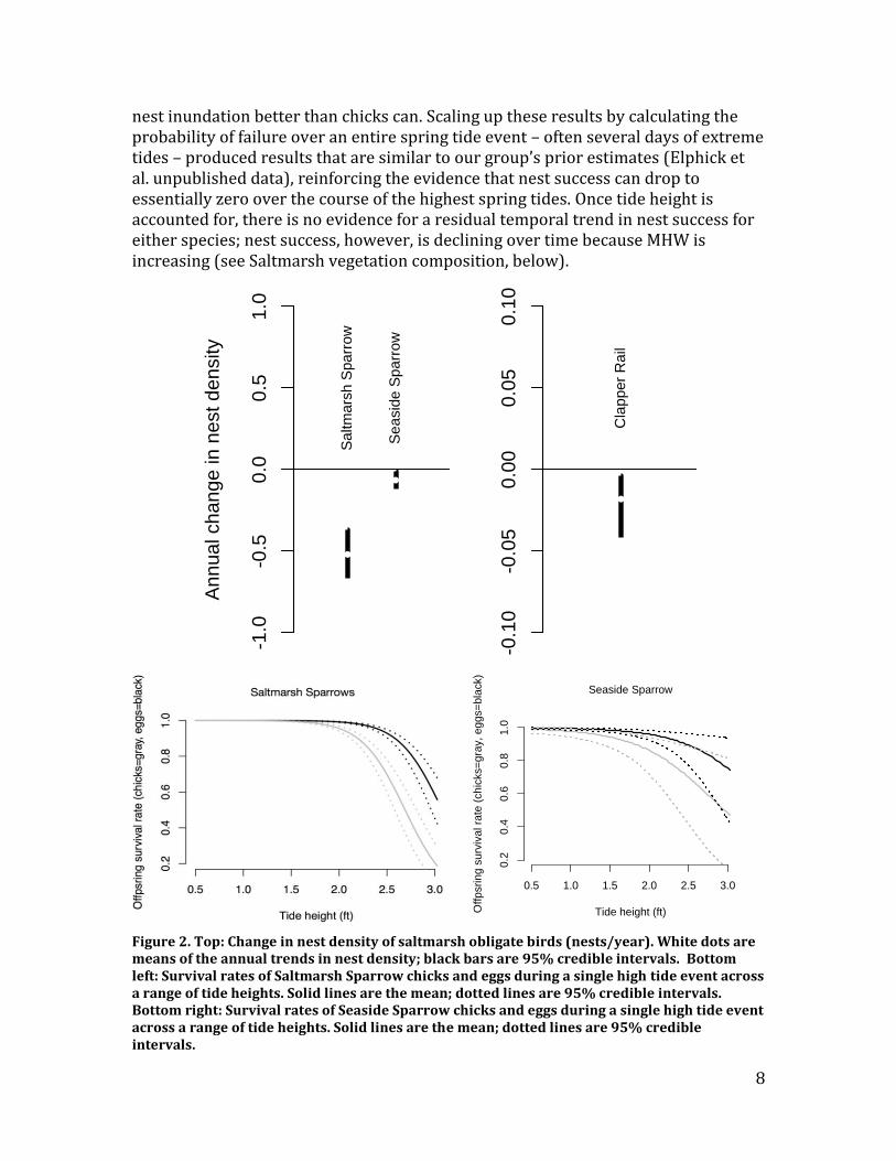
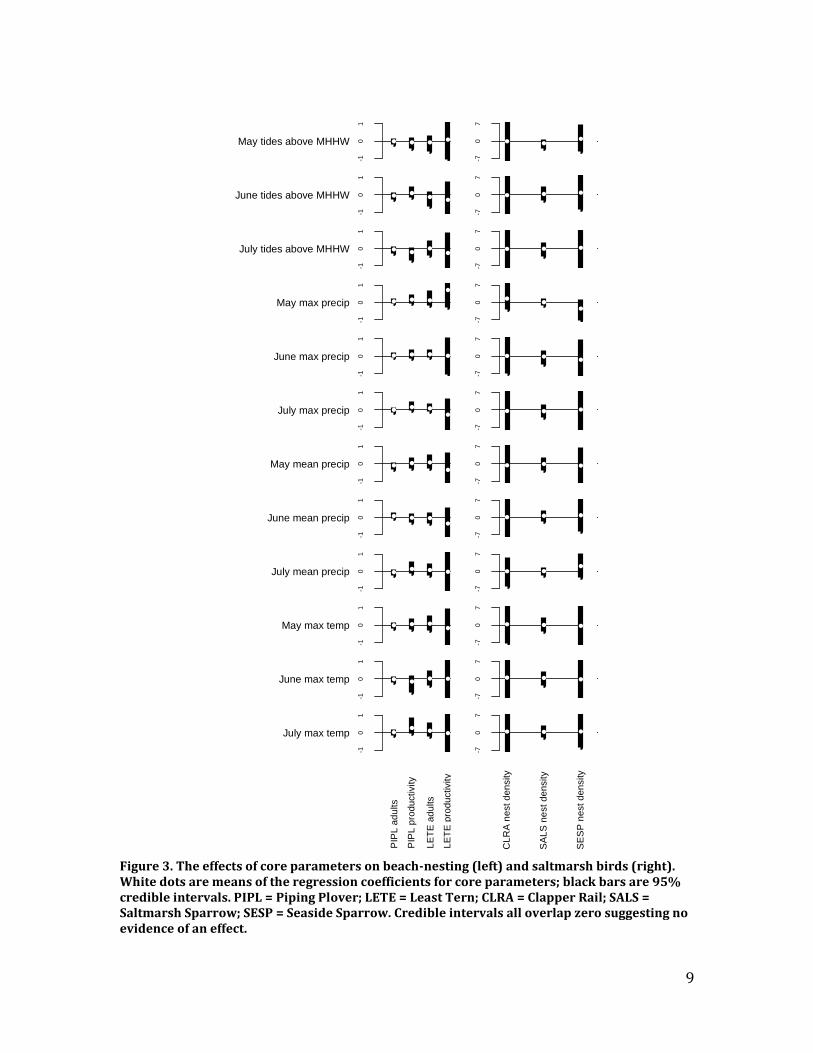
Recommendation – Surveys of specialist saltmarsh bird abundance are an explicit component of SHARP’s larger regional monitoring program, making it possible to place the changes we are observing in LIS into the broader regional context. Given that historic data show clear trends that are consistent with known changes in core parameters, continued monitoring of these variables is likely to provide informative results. A key objective of SHARP is to determine the survey effort – across both space and time – required to detect future trends in specialist saltmarsh bird abundance in order to optimize the cost-effectiveness of future sampling. Saltmarsh bird nesting density, success, and phenology Methods – We compiled data from prior UConn work on specialist saltmarsh bird nesting density and success across Connecticut marshes from 2002-2010 (Gjerdrum et al. 2005, Gjerdrum et al. 2008). We analyzed nest density for Clapper Rail, Saltmarsh Sparrow, and Seaside Sparrow using Bayesian hierarchical models that account for marsh size while estimating temporal trends and the effects of the core parameters. There were not enough Willet nests within standardized plots to estimate density. Because the relationship between Saltmarsh Sparrow nest success and tide height during tidal maxima has been established (Elphick et al. unpublished data), our strategy was to (1) further our understanding of this relationship by increasing the temporal resolution of estimates to examine whether the relationship is evident at smaller temporal scales, and (2) replicate these analyses for other specialist saltmarsh birds, as data allowed. We developed a novel model of nest success that made it possible to estimate the effect of a single high tide on the survival of a single egg or chick in a nest while accounting for any potential autocorrelation between offspring from the same nest. Our model makes it possible to estimate the effect of tide height on nest success at time scales of daily tide events. Because our collection of data on the timing of key events in the life-cycle of saltmarsh birds has only begun recently, we sought additional information from birder records as compiled by eBird. Although this database has considerable potential for tracking phenological shifts in the future, we concluded that it currently lacks adequate data to address these questions for specialist saltmarsh birds. See Migratory shorebirds, below, for more details. Results – The nest density of specialist saltmarsh nesting birds is declining for Saltmarsh Sparrow, Seaside Sparrow, and Clapper Rail, with Saltmarsh Sparrows showing the strongest decline (Figure 2, top). There is no evidence, however, that the core parameters explain the declining trend in nest density (Figure 3). The nest success data were sufficient to conduct analyses for Saltmarsh Sparrow and Seaside Sparrow. Nest success for both species is affected by tide height and this effect is detectable even over the timescale of a single high tide event (Figure 2, bottom). Saltmarsh Sparrow nest success is more strongly affected by tide height, which was expected because, on average, they nest lower in saltmarsh vegetation than Seaside Sparrows (Elphick et al. unpublished data). Both species are more sensitive to flooding during the chick stage suggesting that eggs can survive

8

nest inundation better than chicks can. Scaling up these results by calculating the probability of failure over an entire spring tide event – often several days of extreme tides – produced results that are similar to our group’s prior estimates (Elphick et al. unpublished data), reinforcing the evidence that nest success can drop to essentially zero over the course of the highest spring tides. Once tide height is accounted for, there is no evidence for a residual temporal trend in nest success for either species; nest success, however, is declining over time because MHW is increasing (see Saltmarsh vegetation composition, below).

Figure 2. Top: Change in nest density of saltmarsh obligate birds (nests/year). White dots are means of the annual trends in nest density; black bars are 95% credible intervals. Bottom left: Survival rates of Saltmarsh Sparrow chicks and eggs during a single high tide event across a range of tide heights. Solid lines are the mean; dotted lines are 95% credible intervals. Bottom right: Survival rates of Seaside Sparrow chicks and eggs during a single high tide event across a range of tide heights. Solid lines are the mean; dotted lines are 95% credible intervals.

-1.0

-0.5

0.0

0.5

1.0

An

nua

l ch

an

ge

in

ne

st

den

sity

Sa

ltm

ars

h S

pa

rro

w

Se

asid

e S

pa

rro

w

-0.1

0-0

.05

0.0

00

.05

0.1

0

Cla

pp

er

Ra

il

0.5 1.0 1.5 2.0 2.5 3.0

0.2

0.4

0.6

0.8

1.0

Tide height (ft)Offp

sri

ng

surv

iva

l ra

te (

chic

ks=

gra

y, eg

gs=

bla

ck)

Seaside Sparrow

9

Figure 3. The effects of core parameters on beach-nesting (left) and saltmarsh birds (right). White dots are means of the regression coefficients for core parameters; black bars are 95% credible intervals. PIPL = Piping Plover; LETE = Least Tern; CLRA = Clapper Rail; SALS = Saltmarsh Sparrow; SESP = Seaside Sparrow. Credible intervals all overlap zero suggesting no evidence of an effect.

Beach-nesting birds

May tides above MHHW

-10

1

June tides above MHHW

-10

1

July tides above MHHW

-10

1

May max precip

-10

1

June max precip-1

01

July max precip

-10

1

May mean precip

-10

1

June mean precip

-10

1

July mean precip

-10

1

May max temp

-10

1

June max temp

-10

1

July max temp

-10

1

PIP

L a

du

lts

PIP

L p

rod

uctivity

LE

TE

ad

ults

LE

TE

pro

du

ctivity

Tidal marsh birds

-70

7

-70

7

-70

7

-70

7

-70

7

-70

7

-70

7

-70

7

-70

7

-70

7

-70

7

-70

7

CL

RA

ne

st

de

nsity

SA

LS

ne

st

de

nsity

SE

SP

ne

st

de

nsity

10

Recommendations – Because its relationship with tide height is well-established, Saltmarsh Sparrow nest success can be used as an indicator of the tidal flooding regime of marshes as well as the likely future of nest success for other specialist saltmarsh nesting species, like Seaside Sparrow, Clapper Rail, and Willet. Monitoring Saltmarsh Sparrow nests is relatively inexpensive and could be implemented across large spatial scales, providing data in areas where tidal regime is not currently being monitored. Methods for standardized monitoring of nests and assignment of nest fates exist (SHARP Nest Searching and Monitoring SOP and SHARP Nest Fate Assignment SOP) and are at: http://www.tidalmarshbirds.net/?page_id=1596.

Nest density data for multiple species can be collected with no additional effort where Saltmarsh Sparrow nest monitoring is taking place and provides a measure of population trend that is more directly related to population dynamics. Monitoring nest density is especially important for Saltmarsh Sparrows because abundance estimates from standard surveys do not accurately reflect nest density (Meiman et al. 2012; Elphick et al. unpublished data). Colonial waterbirds Methods – We digitized data collected at waterbird colonies by the United States Fish and Wildlife Service (USFWS), the Connecticut Department of Energy and Environmental Protection (DEEP), and the New York State Department of Environmental Conservation (DEC), covering the time period of 1977-2010 at roughly three-year intervals. We analyzed the LIS-wide population sizes over time for 12 species simultaneously in a multi-species hierarchical model that makes it possible to estimate both the species-level and community-level effects of the core parameters (cf. Sauer and Link 2002). This model also incorporated year effects and allowed for state-specific trends.

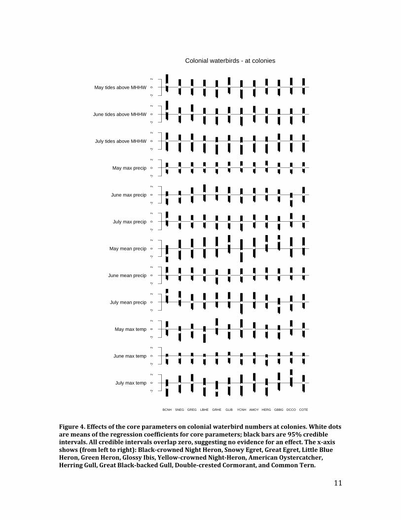
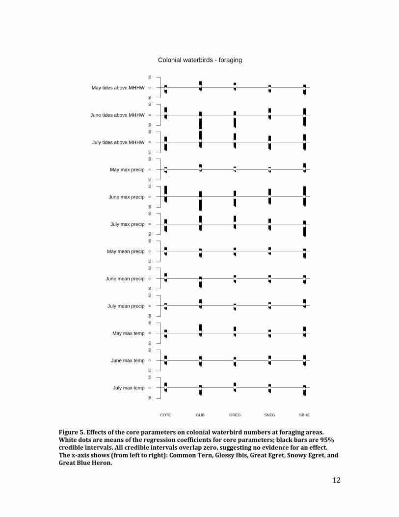
We also conducted an analysis of colonial waterbird distribution and abundance at foraging locations using data that we collected during saltmarsh point counts from 2002-2008. Five species – Great Blue Heron, Great Egret, Snowy Egret, Glossy Ibis, and Common Tern – had enough data from foraging areas to warrant analyses. Results – We did not detect species-level or community-level effects for any of the core parameters at colonies or foraging areas (Figures 4 and 5). We also did not detect population trends at the species-level or community-level. Recommendations – LIS colonial waterbird surveys do not provide information on the effects of the core parameters on coastal island or saltmarsh ecosystems. The community-level analyses serve as an intuitive waterbird index that quantifies the effect of the core parameters on the entire community, but they were not informative here because the core parameters did not have a detectable effect at any level (Figure 6).


11

Figure 4. Effects of the core parameters on colonial waterbird numbers at colonies. White dots are means of the regression coefficients for core parameters; black bars are 95% credible intervals. All credible intervals overlap zero, suggesting no evidence for an effect. The x-axis shows (from left to right): Black-crowned Night Heron, Snowy Egret, Great Egret, Little Blue Heron, Green Heron, Glossy Ibis, Yellow-crowned Night-Heron, American Oystercatcher, Herring Gull, Great Black-backed Gull, Double-crested Cormorant, and Common Tern.

Colonial waterbirds - at colonies


-20

2


-20

2


-20

2

May max precip

-20

2

June max precip

-20

2

July max precip

-20

2

May mean precip

-20

2

June mean precip

-20

2

July mean precip

-20

2

May max temp

-20

2

June max temp

-20

2

July max temp

-20

2

BCNH SNEG GREG LBHE GRHE GLIB YCNH AMOY HERG GBBG DCCO COTE

12

Figure 5. Effects of the core parameters on colonial waterbird numbers at foraging areas. White dots are means of the regression coefficients for core parameters; black bars are 95% credible intervals. All credible intervals overlap zero, suggesting no evidence for an effect. The x-axis shows (from left to right): Common Tern, Glossy Ibis, Great Egret, Snowy Egret, and Great Blue Heron.

Colonial waterbirds - foraging


-50

05

0


-50

05

0


-50

05

0

May max precip

-50

05

0

June max precip

-50

05

0

July max precip

-50

05

0

May mean precip

-50

050

June mean precip

-50

05

0

July mean precip

-50

05

0

May max temp

-50

050

June max temp

-50

05

0

July max temp

-50

05

0

COTE GLIB GREG SNEG GBHE

13

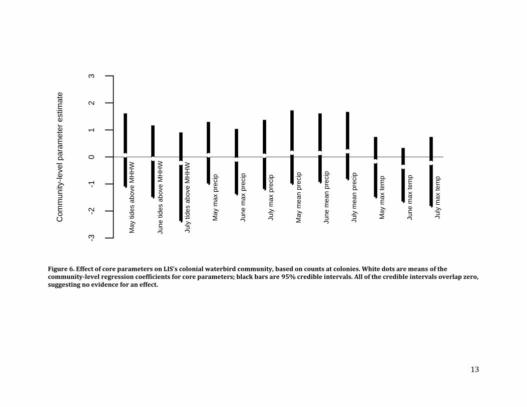
Figure 6. Effect of core parameters on LIS’s colonial waterbird community, based on counts at colonies. White dots are means of the community-level regression coefficients for core parameters; black bars are 95% credible intervals. All of the credible intervals overlap zero, suggesting no evidence for an effect.

-3-2

-10

12

3

Com

mu

nity-le

vel p

ara

me

ter

estim

ate

Ma

y tid

es a

bo

ve M

HH

W

Jun

e t

ides a

bove

MH

HW

Ju

ly tid

es a

bove

MH

HW

Ma

y m

ax p

recip

Jun

e m

ax p

recip

Ju

ly m

ax p

recip

May m

ean

pre

cip

Ju

ne

me

an

pre

cip

July

mea

n p

recip

Ma

y m

ax t

em

p

Jun

e m

ax t

em

p

Ju

ly m

ax te

mp

14

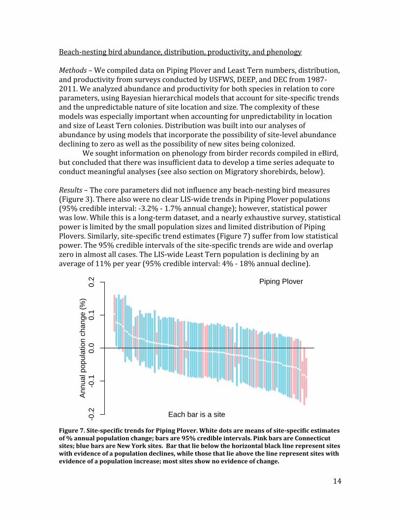
Beach-nesting bird abundance, distribution, productivity, and phenology Methods – We compiled data on Piping Plover and Least Tern numbers, distribution, and productivity from surveys conducted by USFWS, DEEP, and DEC from 1987-2011. We analyzed abundance and productivity for both species in relation to core parameters, using Bayesian hierarchical models that account for site-specific trends and the unpredictable nature of site location and size. The complexity of these models was especially important when accounting for unpredictability in location and size of Least Tern colonies. Distribution was built into our analyses of abundance by using models that incorporate the possibility of site-level abundance declining to zero as well as the possibility of new sites being colonized. We sought information on phenology from birder records compiled in eBird, but concluded that there was insufficient data to develop a time series adequate to conduct meaningful analyses (see also section on Migratory shorebirds, below). Results – The core parameters did not influence any beach-nesting bird measures (Figure 3). There also were no clear LIS-wide trends in Piping Plover populations (95% credible interval: -3.2% - 1.7% annual change); however, statistical power was low. While this is a long-term dataset, and a nearly exhaustive survey, statistical power is limited by the small population sizes and limited distribution of Piping Plovers. Similarly, site-specific trend estimates (Figure 7) suffer from low statistical power. The 95% credible intervals of the site-specific trends are wide and overlap zero in almost all cases. The LIS-wide Least Tern population is declining by an average of 11% per year (95% credible interval: 4% - 18% annual decline).

Figure 7. Site-specific trends for Piping Plover. White dots are means of site-specific estimates of % annual population change; bars are 95% credible intervals. Pink bars are Connecticut sites; blue bars are New York sites. Bar that lie below the horizontal black line represent sites with evidence of a population declines, while those that lie above the line represent sites with evidence of a population increase; most sites show no evidence of change.

-0.2

-0.1

0.0

0.1

0.2

Each bar is a site

Piping Plover

An

nu

al p

op

ula

tio

n c

han

ge (

%)

15

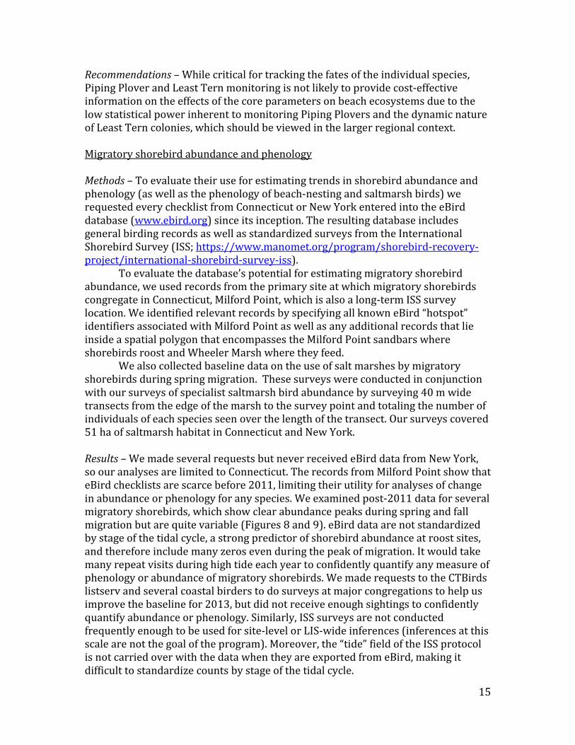
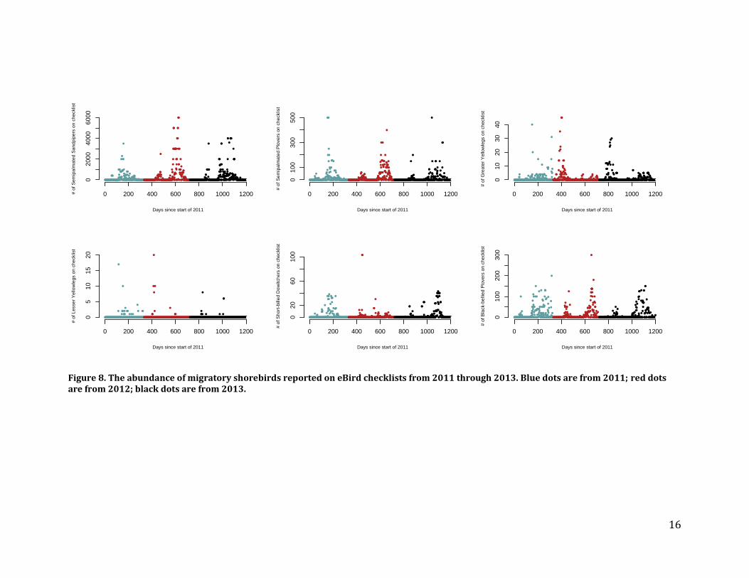
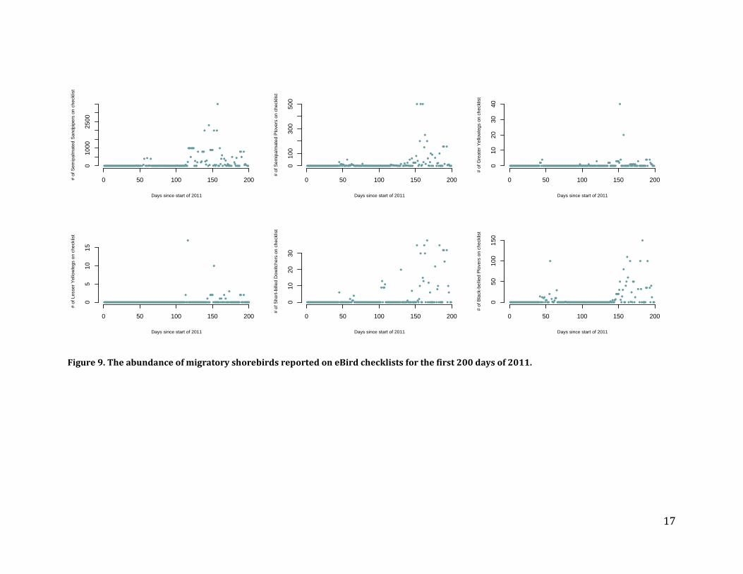
Recommendations – While critical for tracking the fates of the individual species, Piping Plover and Least Tern monitoring is not likely to provide cost-effective information on the effects of the core parameters on beach ecosystems due to the low statistical power inherent to monitoring Piping Plovers and the dynamic nature of Least Tern colonies, which should be viewed in the larger regional context. Migratory shorebird abundance and phenology Methods – To evaluate their use for estimating trends in shorebird abundance and phenology (as well as the phenology of beach-nesting and saltmarsh birds) we requested every checklist from Connecticut or New York entered into the eBird database (www.ebird.org) since its inception. The resulting database includes general birding records as well as standardized surveys from the International Shorebird Survey (ISS; https://www.manomet.org/program/shorebird-recovery-project/international-shorebird-survey-iss). To evaluate the database’s potential for estimating migratory shorebird abundance, we used records from the primary site at which migratory shorebirds congregate in Connecticut, Milford Point, which is also a long-term ISS survey location. We identified relevant records by specifying all known eBird “hotspot” identifiers associated with Milford Point as well as any additional records that lie inside a spatial polygon that encompasses the Milford Point sandbars where shorebirds roost and Wheeler Marsh where they feed. We also collected baseline data on the use of salt marshes by migratory shorebirds during spring migration. These surveys were conducted in conjunction with our surveys of specialist saltmarsh bird abundance by surveying 40 m wide transects from the edge of the marsh to the survey point and totaling the number of individuals of each species seen over the length of the transect. Our surveys covered 51 ha of saltmarsh habitat in Connecticut and New York. Results – We made several requests but never received eBird data from New York, so our analyses are limited to Connecticut. The records from Milford Point show that eBird checklists are scarce before 2011, limiting their utility for analyses of change in abundance or phenology for any species. We examined post-2011 data for several migratory shorebirds, which show clear abundance peaks during spring and fall migration but are quite variable (Figures 8 and 9). eBird data are not standardized by stage of the tidal cycle, a strong predictor of shorebird abundance at roost sites, and therefore include many zeros even during the peak of migration. It would take many repeat visits during high tide each year to confidently quantify any measure of phenology or abundance of migratory shorebirds. We made requests to the CTBirds listserv and several coastal birders to do surveys at major congregations to help us improve the baseline for 2013, but did not receive enough sightings to confidently quantify abundance or phenology. Similarly, ISS surveys are not conducted frequently enough to be used for site-level or LIS-wide inferences (inferences at this scale are not the goal of the program). Moreover, the “tide” field of the ISS protocol is not carried over with the data when they are exported from eBird, making it difficult to standardize counts by stage of the tidal cycle.

http://www.ebird.org/

https://www.manomet.org/program/shorebird-recovery-project/international-shorebird-survey-iss

https://www.manomet.org/program/shorebird-recovery-project/international-shorebird-survey-iss

16

Figure 8. The abundance of migratory shorebirds reported on eBird checklists from 2011 through 2013. Blue dots are from 2011; red dots are from 2012; black dots are from 2013.

0 200 400 600 800 1000 1200

02

00

04

00

06

00

0

Days since start of 2011

# o

f S

em

ipa

lma

ted

Sa

nd

pip

ers

on

ch

ecklis

t

0 200 400 600 800 1000 1200

01

00

30

05

00


# o

f S

em

ipa

lma

ted

Plo

ve

rs o

n c

he

cklis

t

0 200 400 600 800 1000 1200

010

20

30

40


# o

f G

rea

ter

Ye

llow

leg

s o

n c

he

cklis

t

0 200 400 600 800 1000 1200

05

10

15

20


# o

f L

esse

r Y

ello

wle

gs o

n c

he

cklis

t

0 200 400 600 800 1000 1200

02

06

010

0


# o

f S

ho

rt-b

ille

d D

ow

itch

ers

on

ch

ecklis

t

0 200 400 600 800 1000 1200

010

020

030

0


# o

f B

lack-b

elli

ed

Plo

ve

rs o

n c

he

cklis

t

17

Figure 9. The abundance of migratory shorebirds reported on eBird checklists for the first 200 days of 2011.

0 50 100 150 200

010

00

25

00


# o

f S

em

ipa

lma

ted

Sa

nd

pip

ers

on

ch

ecklis

t

0 50 100 150 200

01

00

30

05

00


# o

f S

em

ipa

lma

ted

Plo

ve

rs o

n c

he

cklis

t

0 50 100 150 200

01

02

03

040


# o

f G

rea

ter

Ye

llow

leg

s o

n c

he

cklis

t

0 50 100 150 200

05

10

15


# o

f L

esse

r Y

ello

wle

gs o

n c

he

cklis

t

0 50 100 150 200

01

020

30


# o

f S

ho

rt-b

ille

d D

ow

itch

ers

on

ch

ecklis

t

0 50 100 150 200

05

010

015

0


# o

f B

lack-b

elli

ed

Plo

ve

rs o

n c

he

cklis

t

18

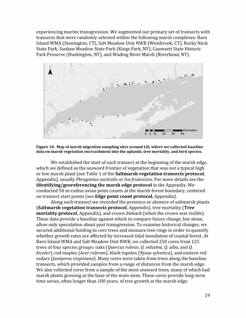
We detected six shorebird species on our saltmarsh transects: Black-bellied Plover, Greater Yellowlegs, Lesser Yellowlegs, Ruddy Turnstone, Least Sandpiper, and Short-billed Dowitcher. Together, these species were found at a density of only 0.375 birds/ha. This low density is driven by the fact that 91% of transects in Connecticut and 100% of transects in New York had zero counts. Recommendations – eBird data will potentially be more useful in the future as longer time series accumulate, but our experience was that gaining access to eBird data can be challenging and should be factored into any planned use. Similarly, our experience suggests that conducting standardized surveys to quantify the abundance or phenology of migratory shorebirds at either statewide or LIS-wide scales would be time intensive relative to the amount of information gained. Our pilot saltmarsh surveys suggest that, relative to the total available area, migratory shorebirds are uncommon in salt marshes during spring migration. Although the total numbers of shorebirds in marshes are not inconsequential, the low densities and high frequency of zero counts, means that high sampling rates will be required to make informative estimates. Our surveys will function as a baseline, which is important as there are no other systematic surveys of migrant shorebirds throughout LIS salt marshes. We recommend, however, that any future monitoring should be stratified by habitats – with a focus on increased sampling in sub-habitats where shorebirds are more likely to be found (e.g., pannes). Overall, the results suggest that sentinel monitoring focused on shorebirds will require a much larger data collection effort than was possible in the current project. LISS sentinel (v): Species composition within coastal forests, shrublands, and grasslands. The following measures all relate to baseline data collection, which we developed from transects conducted at the marsh-to-forest boundary in Connecticut and New York during 2013 (Elphick and Field 2014). We established 170 transects across both shores of LIS that can be resurveyed in the future (Figure 10). We georeferenced the start points of each transect using the average of at least three GPS readings and by drawing the start point on color aerial photographs, which we subsequently scanned and archived. At Barn Island Wildlife Management Area (WMA) and the Salt Meadow Unit of Stewart B. McKinney National Wildlife Refuge (NWR), we marked trees along transects with aluminum tags, providing another method for relocating transects in the future. We took the bearing of each transect, relative to true north, to the nearest degree. We randomly located transects in areas that were most likely to be experiencing marine transgression, which we identified by finding areas that had a slope of less than 3.5 degrees over the first 10 m (equivalent to an elevation change of two feet or less, which was chosen because the current digital elevation models estimate elevation at one foot intervals). Because a large part of the LIS coast is privately owned, many transects fell on private land. We obtained permission for private land and only dropped transects from the study when we were denied permission, which was rare. As a result, the data obtained from these transects should be representative of LIS areas that are most likely to be

19

experiencing marine transgression. We augmented our primary set of transects with transects that were randomly selected within the following marsh complexes: Barn Island WMA (Stonington, CT), Salt Meadow Unit NWR (Westbrook, CT), Rocky Neck State Park, Sunken Meadow State Park (Kings Park, NY), Caumsett State Historic Park Preserve (Huntington, NY), and Wading River Marsh (Riverhead, NY).

Figure 10. Map of marsh migration sampling sites around LIS, where we collected baseline data on marsh vegetation encroachment into the uplands, tree mortality, and bird species.

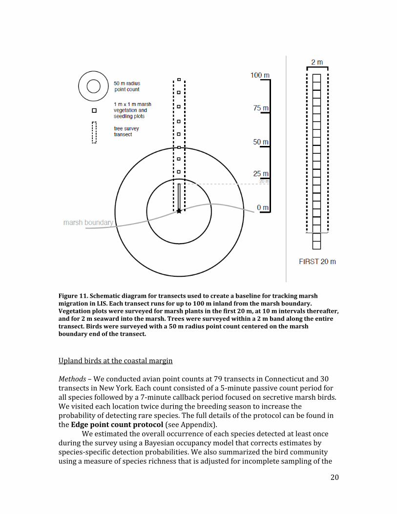
We established the start of each transect at the beginning of the marsh edge,

which we defined as the seaward frontier of vegetation that was not a typical high or low marsh plant (see Table 1 of the Saltmarsh vegetation transects protocol, Appendix), usually Phragmites australis or Iva frutescens. For more details see the Identifying/georeferencing the marsh edge protocol in the Appendix. We conducted 50 m-radius avian point counts at the marsh-forest boundary, centered on transect start points (see Edge point count protocol, Appendix).

Along each transect we recorded the presence or absence of saltmarsh plants (Saltmarsh vegetation transects protocol, Appendix), tree mortality (Tree mortality protocol, Appendix), and crown dieback (when the crown was visible). These data provide a baseline against which to compare future change, but alone, allow only speculation about past transgression. To examine historical changes, we secured additional funding to core trees and measure tree rings in order to quantify whether growth rates are affected by increased tidal inundation of coastal forest. At Barn Island WMA and Salt Meadow Unit NWR, we collected 250 cores from 125 trees of four species groups: oaks (Quercus rubrus, Q. velutina, Q. alba, and Q. bicolor), red maples (Acer rubrum), black tupelos (Nyssa sylvatica), and eastern red cedars (Juniperus virginiana). Many cores were taken from trees along the baseline transects, which provided samples from a range of distances from the marsh edge. We also collected cores from a sample of the most seaward trees, many of which had marsh plants growing at the base of the main stem. These cores provide long-term time series, often longer than 100 years, of tree growth at the marsh edge.

20

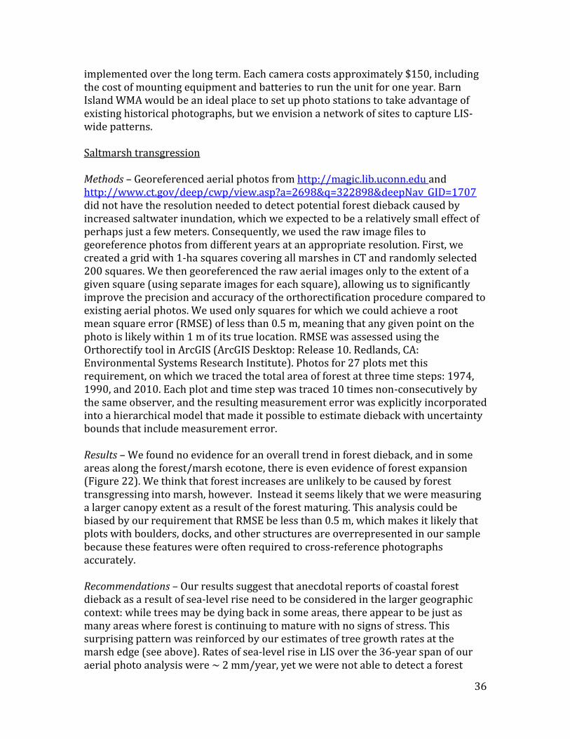
Figure 11. Schematic diagram for transects used to create a baseline for tracking marsh migration in LIS. Each transect runs for up to 100 m inland from the marsh boundary. Vegetation plots were surveyed for marsh plants in the first 20 m, at 10 m intervals thereafter, and for 2 m seaward into the marsh. Trees were surveyed within a 2 m band along the entire transect. Birds were surveyed with a 50 m radius point count centered on the marsh boundary end of the transect.

Upland birds at the coastal margin Methods – We conducted avian point counts at 79 transects in Connecticut and 30 transects in New York. Each count consisted of a 5-minute passive count period for all species followed by a 7-minute callback period focused on secretive marsh birds. We visited each location twice during the breeding season to increase the probability of detecting rare species. The full details of the protocol can be found in the Edge point count protocol (see Appendix). We estimated the overall occurrence of each species detected at least once during the survey using a Bayesian occupancy model that corrects estimates by species-specific detection probabilities. We also summarized the bird community using a measure of species richness that is adjusted for incomplete sampling of the

21

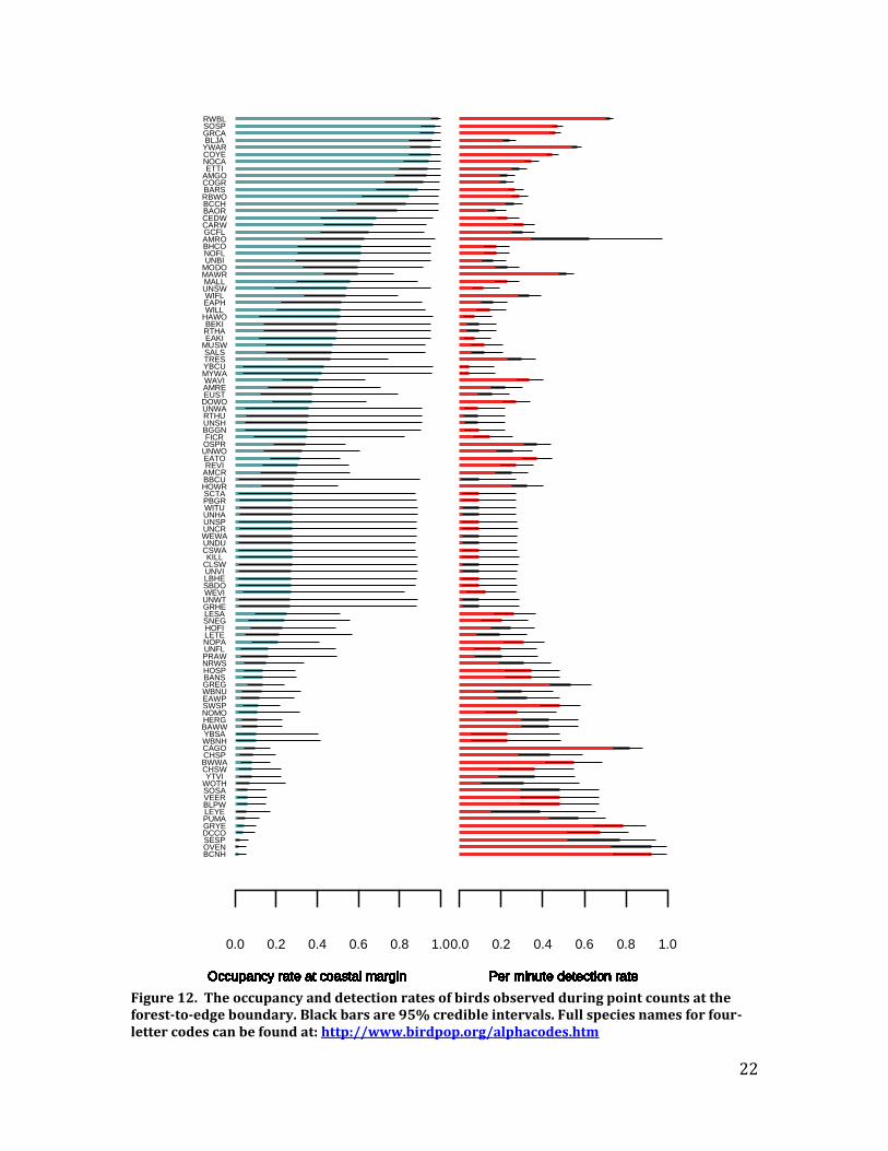
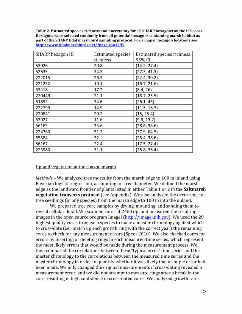
community. We estimated species richness of upland birds at the coastal margin within the randomly-selected hexagons chosen for the Saltmarsh Habitat and Avian Research Program (see http://www.tidalmarshbirds.net/?page_id=1295). We corrected hexagon-wide species richness estimates for incomplete sampling using the Chao 2 non-parametric estimator (Chao 1987). Average upland bird species richness was modeled across LIS using conjugate distribution sampling (Gelman et al. 2004). This approach makes it possible to estimate the lower and upper bounds on species richness in areas that were not sampled. Using a non-parametric estimator with conjugate distribution sampling also means that the entire analysis can be carried out using only a few lines of code in the most basic version of the open source software R (http://www.r-project.org). As a result, it will be possible for others to update the model in almost real-time if additional point counts are conducted. This flexibility would allow for rapid assessments of the bird community before any potential management actions are implemented at the forest-to-marsh boundary. Results – The most common species (occurrence rates of 0.8 or greater) were, in order of occurrence: Red-winged Blackbird, Song Sparrow, Gray Catbird, Blue Jay, Yellow Warbler, Common Yellowthroat, Northern Cardinal, Tufted Titmouse, American Goldfinch, Common Grackle, Barn Swallow, Red-bellied Woodpecker, and Black-capped Chickadee (Figure 12). All of these species are common and widespread in Connecticut, and most are not declining (www.ctbirdtrends.org); Blue Jay and Red-winged Blackbird do have negative trends, but are sufficiently abundant locally and globally that they are not a conservation concern. In general, specialist saltmarsh birds were less common than upland birds at the marsh edge. Estimated occurrence of Saltmarsh Sparrows was ~ 0.5 and estimated occurrence of Seaside Sparrows was < 0.1. Recommendations – Historical data lacked sufficient spatial resolution for comparison so it is impossible to judge how well change in these variables will reflect change in core parameters. Nonetheless, our upland edge surveys provide a baseline for future assessments of the effects of climate change and can be used to assess future change and to examine geographic variation in species occurrence and richness (Table 2). Occupancy estimates for upland birds also will be incorporated into conservation planning assessments currently being developed by C. Field, making it possible for land managers to avoid areas of high species richness if management actions (such as tree cutting or girdling) at the coastal margin are implemented. Our data suggest, however, that there are not severe trade-offs between upland and tidal marsh Greatest Conservation Needs (GCN) species, as most upland GCN species have very low occupancy rates at the coastal margin (Figure 12).


http://www.r-project.org/

http://www.ctbirdtrends.org/

22

Figure 12. The occupancy and detection rates of birds observed during point counts at the forest-to-edge boundary. Black bars are 95% credible intervals. Full species names for four-letter codes can be found at: http://www.birdpop.org/alphacodes.htm

0.0 0.2 0.4 0.6 0.8 1.0

BCNH

Occupancy rate at coastal margin

OVEN


SESP


DCCO


GRYE


PUMA


LEYE


BLPW


VEER


SOSA


WOTH


YTVI


CHSW


BWWA


CHSP


CAGO


WBNH


YBSA


BAWW


HERG


NOMO


SWSP


EAWP


WBNU


GREG


BANS


HOSP


NRWS


PRAW


UNFL


NOPA


LETE


HOFI


SNEG


LESA


GRHE


UNWT


WEVI


SBDO


LBHE


UNVI


CLSW


KILL


CSWA


UNDU


WEWA


UNCR


UNSP


UNHA


WITU


PBGR


SCTA


HOWR


BBCU


AMCR


REVI


EATO


UNWO


OSPR


FICR


BGGN


UNSH


RTHU


UNWA


DOWO


EUST


AMRE


WAVI


MYWA


YBCU


TRES


SALS


MUSW


EAKI


RTHA


BEKI


HAWO


WILL


EAPH


WIFL


UNSW


MALL


MAWR


MODO


UNBI


NOFL


BHCO


AMRO


GCFL


CARW


CEDW


BAOR


BCCH


RBWO


BARS


COGR


AMGO


ETTI


NOCA


COYE


YWAR


BLJA


GRCA


SOSP


RWBL


0.0 0.2 0.4 0.6 0.8 1.0

Per minute detection ratePer minute detection ratePer minute detection ratePer minute detection ratePer minute detection ratePer minute detection ratePer minute detection ratePer minute detection ratePer minute detection ratePer minute detection ratePer minute detection ratePer minute detection ratePer minute detection ratePer minute detection ratePer minute detection ratePer minute detection ratePer minute detection ratePer minute detection ratePer minute detection ratePer minute detection ratePer minute detection ratePer minute detection ratePer minute detection ratePer minute detection ratePer minute detection ratePer minute detection ratePer minute detection ratePer minute detection ratePer minute detection ratePer minute detection ratePer minute detection ratePer minute detection ratePer minute detection ratePer minute detection ratePer minute detection ratePer minute detection ratePer minute detection ratePer minute detection ratePer minute detection ratePer minute detection ratePer minute detection ratePer minute detection ratePer minute detection ratePer minute detection ratePer minute detection ratePer minute detection ratePer minute detection ratePer minute detection ratePer minute detection ratePer minute detection ratePer minute detection ratePer minute detection ratePer minute detection ratePer minute detection ratePer minute detection ratePer minute detection ratePer minute detection ratePer minute detection ratePer minute detection ratePer minute detection ratePer minute detection ratePer minute detection ratePer minute detection ratePer minute detection ratePer minute detection ratePer minute detection ratePer minute detection ratePer minute detection ratePer minute detection ratePer minute detection ratePer minute detection ratePer minute detection ratePer minute detection ratePer minute detection ratePer minute detection ratePer minute detection ratePer minute detection ratePer minute detection ratePer minute detection ratePer minute detection ratePer minute detection ratePer minute detection ratePer minute detection ratePer minute detection ratePer minute detection ratePer minute detection ratePer minute detection ratePer minute detection ratePer minute detection ratePer minute detection ratePer minute detection ratePer minute detection ratePer minute detection ratePer minute detection ratePer minute detection ratePer minute detection ratePer minute detection ratePer minute detection ratePer minute detection ratePer minute detection ratePer minute detection ratePer minute detection ratePer minute detection ratePer minute detection ratePer minute detection rate

http://www.birdpop.org/alphacodes.htm

23

Table 2. Estimated species richness and uncertainty for 15 SHARP hexagons on the LIS coast. Hexagons were selected randomly from all potential hexagons containing marsh habitat as part of the SHARP tidal marsh bird sampling protocol. For a map of hexagon locations see http://www.tidalmarshbirds.net/?page_id=1295.

SHARP hexagon ID Estimated species richness

Estimated species richness 95% CI

53026 20.8 (14.2, 27.4)

52635 34.3 (27.3, 41.3)

222015 26.3 (22.4, 30.2)

221232 19.1 (16.7, 21.6)

53418 17.2 (8.4, 26)

220449 21.1 (18.7, 23.5)

51852 34.6 (26.1, 43)

222799 14.9 (11.5, 18.3)

220841 20.2 (15, 25.4)

53027 11.6 (9.9, 13.2)

56165 33.6 (28.6, 38.6)

224763 51.2 (37.9, 64.5)

55384 32 (25.4, 38.6)

56167 22.4 (17.5, 27.4)

223980 31.1 (25.8, 36.4)

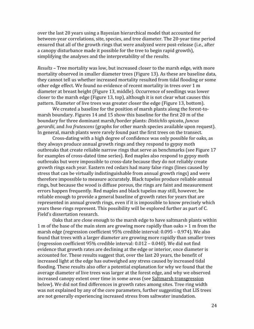
Upland vegetation at the coastal margin Methods – We analyzed tree mortality from the marsh edge to 100 m inland using Bayesian logistic regression, accounting for tree diameter. We defined the marsh edge as the landward frontier of plants listed in either Table 1 or 2 in the Saltmarsh vegetation transects protocol (see Appendix). We also analyzed the occurrence of tree seedlings (of any species) from the marsh edge to 100 m into the upland. We prepared tree core samples by drying, mounting, and sanding them to reveal cellular detail. We scanned cores at 2400 dpi and measured the resulting images in the open source program ImageJ (http://imagej.nih.gov). We used the 20 highest quality cores from each species to make a master chronology against which to cross-date (i.e., match up each growth ring with the correct year) the remaining cores to check for any measurement errors (Speer 2010). We also checked cores for errors by inserting or deleting rings in each measured time series, which represent the most likely errors that would be made during the measurement process. We then compared the correlations between these “typical error” time series and the master chronology to the correlations between the measured time series and the master chronology in order to quantify whether it was likely that a simple error had been made. We only changed the original measurements if cross-dating revealed a measurement error, and we did not attempt to measure rings after a break in the core, resulting in high confidence in cross-dated cores. We analyzed growth rates


http://imagej.nih.gov/

24

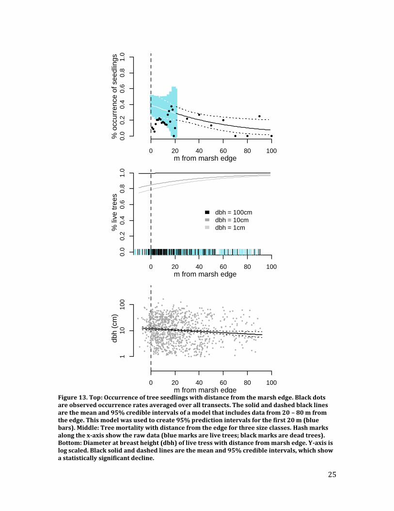
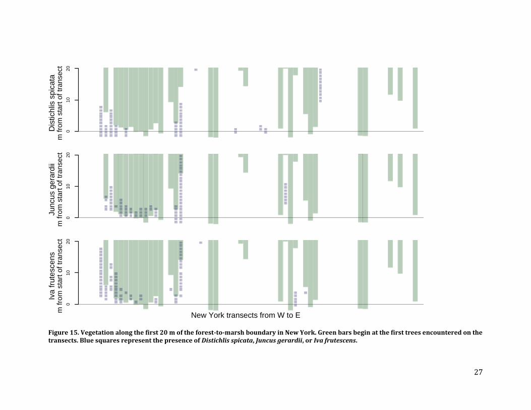
over the last 20 years using a Bayesian hierarchical model that accounted for between-year correlations, site, species, and tree diameter. The 20-year time period ensured that all of the growth rings that were analyzed were post-release (i.e., after a canopy disturbance made it possible for the tree to begin rapid growth), simplifying the analyses and the interpretability of the results. Results – Tree mortality was low, but increased closer to the marsh edge, with more mortality observed in smaller diameter trees (Figure 13). As these are baseline data, they cannot tell us whether increased mortality resulted from tidal flooding or some other edge effect. We found no evidence of recent mortality in trees over 1 m diameter at breast height (Figure 13, middle). Occurrence of seedlings was lower closer to the marsh edge (Figure 13, top), although it is not clear what causes this pattern. Diameter of live trees was greater closer the edge (Figure 13, bottom). We created a baseline for the position of marsh plants along the forest-to-marsh boundary. Figures 14 and 15 show this baseline for the first 20 m of the boundary for three dominant marsh/border plants: Distichlis spicata, Juncus gerardii, and Iva frutescens (graphs for other marsh species available upon request). In general, marsh plants were rarely found past the first trees on the transect.

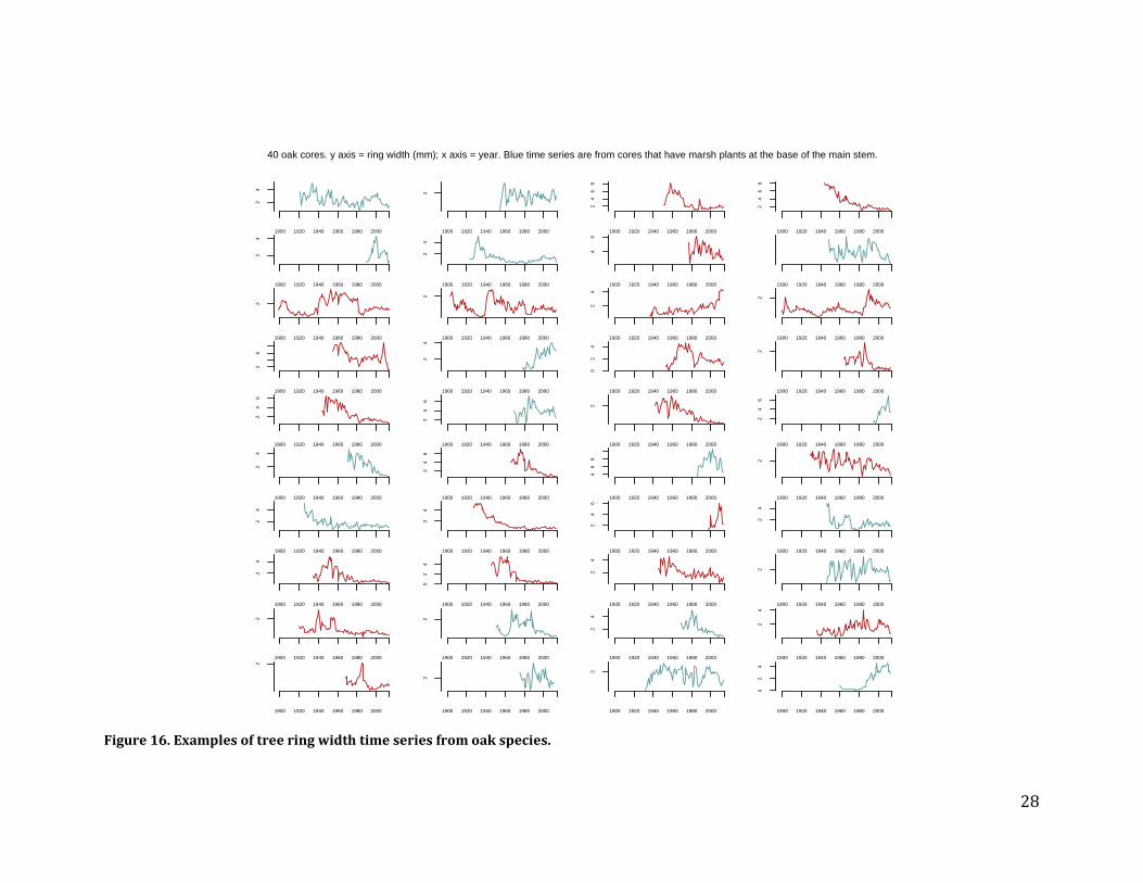
Cross-dating with a high degree of confidence was only possible for oaks, as they always produce annual growth rings and they respond to gypsy moth outbreaks that create reliable narrow rings that serve as benchmarks (see Figure 17 for examples of cross-dated time series). Red maples also respond to gypsy moth outbreaks but were impossible to cross-date because they do not reliably create growth rings each year. Eastern red cedars had many false rings (lines caused by stress that can be virtually indistinguishable from annual growth rings) and were therefore impossible to measure accurately. Black tupelos produce reliable annual rings, but because the wood is diffuse porous, the rings are faint and measurement errors happen frequently. Red maples and black tupelos may still, however, be reliable enough to provide a general baseline of growth rates for years that are represented in annual growth rings, even if it is impossible to know precisely which years these rings represent. This possibility will be explored further as part of C. Field’s dissertation research. Oaks that are close enough to the marsh edge to have saltmarsh plants within 1 m of the base of the main stem are growing more rapidly than oaks > 1 m from the marsh edge (regression coefficient 95% credible interval: 0.095 – 0.974). We also found that trees with a larger diameter are growing more rapidly than smaller trees (regression coefficient 95% credible interval: 0.012 – 0.040). We did not find evidence that growth rates are declining at the edge or interior, once diameter is accounted for. These results suggest that, over the last 20 years, the benefit of increased light at the edge has outweighed any stress caused by increased tidal flooding. These results also offer a potential explanation for why we found that the average diameter of live trees was larger at the forest edge, and why we observed increased canopy extent over time in some areas (see Saltmarsh transgression below). We did not find differences in growth rates among sites. Tree ring width was not explained by any of the core parameters, further suggesting that LIS trees are not generally experiencing increased stress from saltwater inundation.

25

Figure 13. Top: Occurrence of tree seedlings with distance from the marsh edge. Black dots are observed occurrence rates averaged over all transects. The solid and dashed black lines are the mean and 95% credible intervals of a model that includes data from 20 – 80 m from the edge. This model was used to create 95% prediction intervals for the first 20 m (blue bars). Middle: Tree mortality with distance from the edge for three size classes. Hash marks along the x-axis show the raw data (blue marks are live trees; black marks are dead trees). Bottom: Diameter at breast height (dbh) of live tress with distance from marsh edge. Y-axis is log scaled. Black solid and dashed lines are the mean and 95% credible intervals, which show a statistically significant decline.

0 20 40 60 80 100

0.0

0.2

0.4

0.6

0.8

1.0

m from marsh edge

% o

ccu

rre

nce

of se

ed

lings

0 20 40 60 80 100

0.0

0.2

0.4

0.6

0.8

1.0

m from marsh edge

| | | | ||||| || ||||| || ||||| | ||| || || | | | |||||||||||||||||| | | ||| | ||| ||| || |||| || | || ||||||||||||| || |||| || || || | | | || |||| ||| | | |||| | | ||| |||| | ||||||| | || | | | ||||| | | ||||| | || | || || | | | | ||| | ||||| | | || ||||||||||| | || | | ||||| ||| || | | ||| | || | | || || | | | |||||||| ||| || || || || |||| ||| | | || ||| | ||| ||| ||||| | ||| | |||||||||| |||||||||||||||||||||||||||||| || || || ||| ||||||| | | | | | ||| ||||| ||||| || ||||||||| |||||| | | | | | | | | | | | | | | | ||| || || | | || ||||| | || | | || | | || | | | ||| || || | | || || | ||| || | |||| | ||| || | | ||||| | | ||||||||||||| | | | | || | | ||||| | || || |||||| |||||||||| | | |||| ||||| | | || | || | | | || || ||| ||| || | ||| |||| ||| | | || | | | | | || || | || | | ||| | | || | | | | | | || | || | |||| | || | | | || | || | ||| | | | | || | || || | | | ||| | | | | | | | || || | ||||| | | | | ||| | || || | || | || | | | | || | | ||| || ||| | | | || | |||| || || | ||| | | | |||| | | | | || |||| |||||| ||||| || || | | || | | ||| | | || || | ||| |||| | || | | || | ||||| | ||| || ||||| ||||| ||||| | || || || | ||| |||||||| | |||| |||||| |||| |||| || | | || || |||||| ||| ||||| | | || | | || ||| | |||| ||| ||| | | || | ||| || | | | | ||| | |||| || || | | | |||| | | || | || |||| |||| || |||| | ||| ||| | || |||| | || | | || || | | | | |||| | | ||||| |||||| |||| ||| | ||||| ||| | |||| | || | | || |||| || | | || || || | || | |||| | || ||| || |||| | || || | || |||| | || || | | ||| || | ||| | | || || |||| | | || | | ||| || || ||| | || ||| | ||| ||||||| || | | | ||| | | | | | | |

% liv

e tre

es

dbh = 100cm

dbh = 10cm

dbh = 1cm

0 20 40 60 80 100

db

h (

cm

)

110

10

0

m from marsh edge

dbh

(cm

)

26

Figure 14. Vegetation along the first 20 m of the forest-to-marsh boundary in Connecticut. Green bars begin at the first trees encountered on the transects. Blue squares represent the presence of Distichlis spicata, Juncus gerardii, or Iva frutescens.

Index

01

02

0

Dis

tichlis

sp

icata

m f

rom

sta

rt o

f tr

an

sect

Index

01

02

0

Juncu

s g

era

rdii

m f

rom

sta

rt o

f tr

an

sect

01

02

0

Connecticut transects from W to E

Iva fru

tescens

m f

rom

sta

rt o

f tr

an

sect

27

Figure 15. Vegetation along the first 20 m of the forest-to-marsh boundary in New York. Green bars begin at the first trees encountered on the transects. Blue squares represent the presence of Distichlis spicata, Juncus gerardii, or Iva frutescens.

Index

01

02

0

Dis

tichlis

sp

icata

m f

rom

sta

rt o

f tr

an

sect

Index

01

02

0

Juncu

s g

era

rdii

m f

rom

sta

rt o

f tr

an

sect

01

02

0

New York transects from W to E

Iva fru

tescens

m f

rom

sta

rt o

f tr

an

sect

28

Figure 16. Examples of tree ring width time series from oak species.

Index

40 oak cores. y axis = ring width (mm); x axis = year. Blue time series are from cores that have marsh plants at the base of the main stem.

1900 1920 1940 1960 1980 2000

24

1900 1920 1940 1960 1980 2000

2

1900 1920 1940 1960 1980 2000

24

68

1900 1920 1940 1960 1980 2000

24

68

1900 1920 1940 1960 1980 2000

24

1900 1920 1940 1960 1980 2000

24

1900 1920 1940 1960 1980 2000

46

1900 1920 1940 1960 1980 2000

1900 1920 1940 1960 1980 2000

2

1900 1920 1940 1960 1980 2000

2

1900 1920 1940 1960 1980 2000

24

1900 1920 1940 1960 1980 2000

2

1900 1920 1940 1960 1980 2000

26

1900 1920 1940 1960 1980 2000

24

1900 1920 1940 1960 1980 2000

02

4

1900 1920 1940 1960 1980 2000

2

1900 1920 1940 1960 1980 2000

24

6

1900 1920 1940 1960 1980 2000

24

6

1900 1920 1940 1960 1980 2000

2

1900 1920 1940 1960 1980 2000

24

6

1900 1920 1940 1960 1980 2000

24

1900 1920 1940 1960 1980 2000

24

6

1900 1920 1940 1960 1980 2000

46

8

1900 1920 1940 1960 1980 2000

2

1900 1920 1940 1960 1980 2000

24

1900 1920 1940 1960 1980 2000

24

1900 1920 1940 1960 1980 2000

24

6

1900 1920 1940 1960 1980 2000

24

1900 1920 1940 1960 1980 2000

24

1900 1920 1940 1960 1980 2000

02

4

1900 1920 1940 1960 1980 2000

24

1900 1920 1940 1960 1980 2000

2

1900 1920 1940 1960 1980 2000

2

1900 1920 1940 1960 1980 2000

2

1900 1920 1940 1960 1980 2000

24

1900 1920 1940 1960 1980 2000

24

1900 1920 1940 1960 1980 2000

2

1900 1920 1940 1960 1980 2000

2

1900 1920 1940 1960 1980 2000

2

1900 1920 1940 1960 1980 2000

02

4

29

Recommendations – The data from the 170 baseline transects will make it possible to estimate LIS-wide rates of tree mortality and marsh plant transgression into the upland when they are resurveyed. Because these are the first regional-scale data on marine transgression in LIS, it is difficult to know how frequently sites should be resurveyed. Between five and ten years is likely a reasonable benchmark for the first resurvey given the evidence presented for sentinels (v) and (vi), which suggests that marine transgression is a relatively slow process in this region.

Tree cores are a cost-effective method for obtaining longer time series that track the resilience of the forest-to-marsh boundary. Future sampling should focus on oaks, which are dominant in the forest-edge community and produce reliable annual growth rings that are easy to distinguish and measure with little training. We recommend taking tree cores from other sites, ideally where elevation of the marsh-to-forest boundary is known, to explore whether the resilience of coastal forest observed at Barn Island WMA and Salt Meadow Unit NWR is representative of LIS as a whole. It is possible to quantify differences in growth rates between trees at the marsh edge and trees farther into the forest using ~ 20 trees in each sample. LISS sentinel (vi): Aerial extent, diversity, composition, and marine transgression of salt marshes. The measures for LISS sentinel (vi) consist of only two or three time points because of the limited availability of historical data at the relevant scales. As such, the following measures were not analyzed with respect to the core parameters because such analyses would require more complete time series. Saltmarsh vegetation composition Methods – We compiled historical data on saltmarsh vegetation collected by our group in 2002-2004. These data came from 55 1-ha plots in eight marsh complexes in Connecticut that were initially studied to describe nest site selection in tidal marsh birds (Gjerdrum et al. 2005). The focal marshes include most of the largest in the state and plots were randomly selected from all habitat that could plausibly be used by marsh-nesting sparrows; only extensive Phragmites stands and open water were excluded. Thus, the data are likely to be representative of Connecticut marshes. To assess vegetation change, we resampled these plots in 2013. Before plots were resurveyed, we conducted a statistical power analysis to determine how many samples would be needed from each historical plot to detect changes over the 11-year period. The resulting design had the power to distinguish a ± 5% change in either direction at the 1-ha scale with 95% confidence. We collected all 2013 data during the first three weeks of August, the same sampling period as in 2002-2004.

We also collected vegetation data at 65 locations where we encountered existing equipment, such as PVC wells and wooden stakes, that had been installed in the marsh by other researchers but that was no longer in use. This sample will provide finer resolution data (1 m-squared plots) at points that can be easily re-found and resurveyed in future years without expensive GIS equipment and with considerably less effort than it takes to get trend estimates at the 1-ha scale. It

30

should be noted, however, that these 1 m-squared plots are not a random sample and therefore are not necessarily representative of Connecticut marshes. To facilitate future sampling, we have created a standardized protocol for surveying marsh vegetation aimed at detecting changes in vegetation distributions over time (Saltmarsh vegetation resurvey protocol, Appendix).

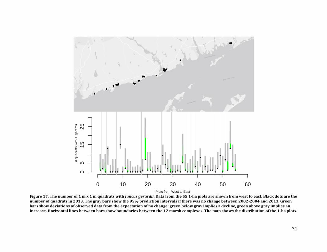
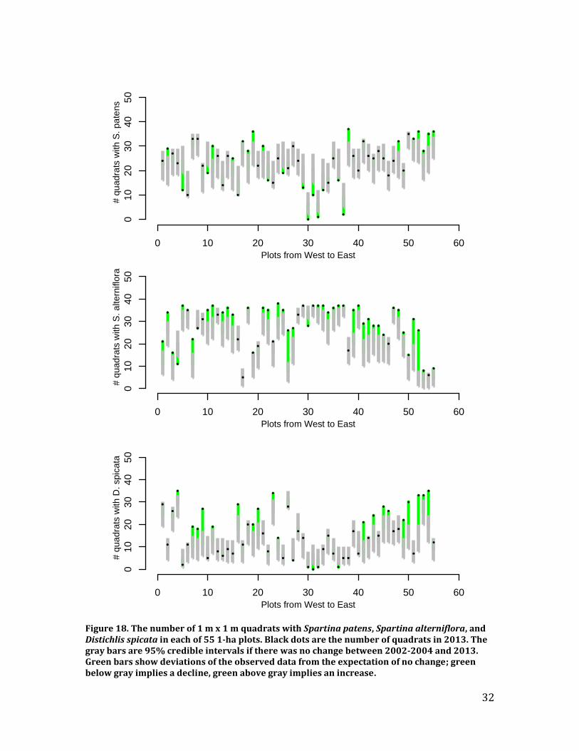
We analyzed data in a Bayesian hierarchical framework that makes it possible to account for site and plot effects while estimating 10-year trends for the four dominant saltmarsh plants: Spartina patens, Spartina alterniflora, Distichlis spicata, and Juncus gerardii. Results – We found that Juncus gerardii, a high marsh species, is becoming less widespread while Spartina alterniflora, a low marsh species, is becoming more widespread (Figures 17-19). Spartina patens, which is the dominant high marsh species, although not at the highest elevations, is increasing in some areas while decreasing in others. Disitchlis spicata, a salt-tolerant pioneer species, increased in most plots (Figures 18 and 19). This increase might be caused by increases in salt concentration and/or the amount of de-vegetated habitat in recent years, potentially caused by storm surges during Hurricanes Irene and Sandy.

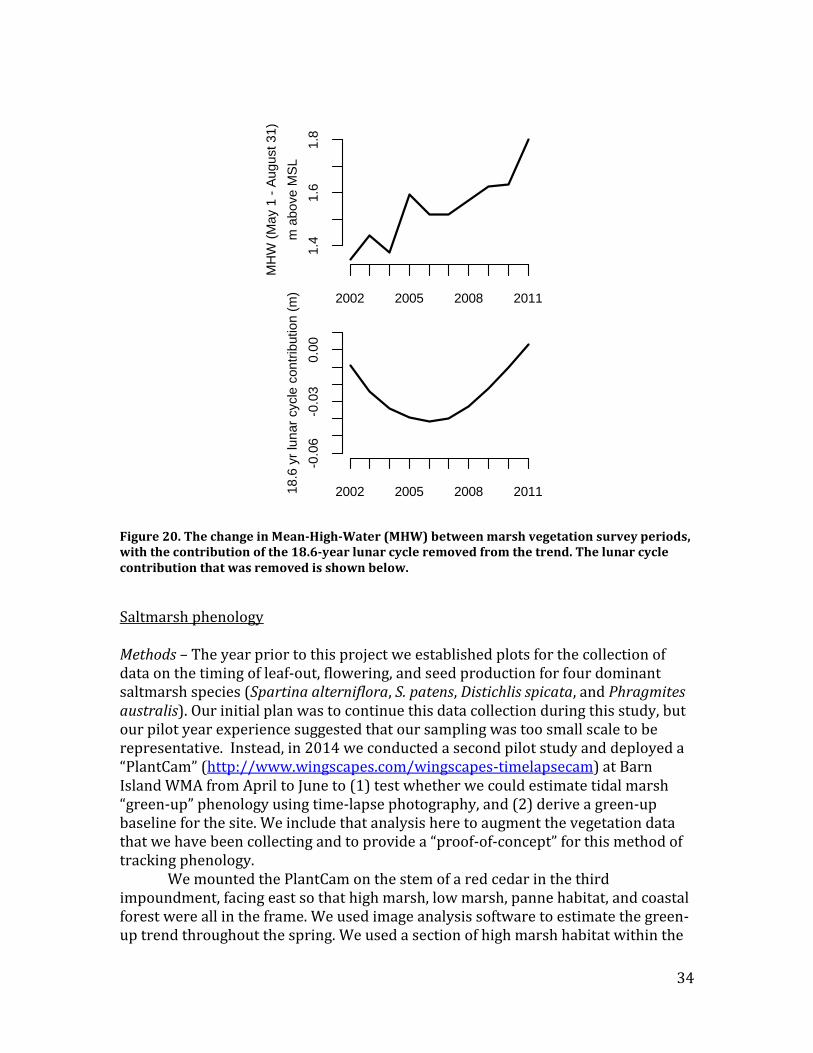
Potentially confounding factors that might explain the saltmarsh vegetation trends are the 18.6-year lunar cycle, which results in changes in peak tide heights (Ivan et al. 2011), and the effects of hurricanes on marsh elevation (Morton and Barras 2011). The nodal cycle, however, has a trivial contribution to total inundation hours of salt marshes compared to the overall trend in Mean-High-Water (MHW), and so is unlikely to account for substantial vegetation changes across the marsh surface (Figure 20). Recommendations – The decline of Juncus gerardii and the increase of Spartina alterniflora across almost every plot sampled in eight different marsh systems spread out along the Connecticut coast suggests that sea-level rise is causing marshes to get wetter over timescales as short as a decade. Our results are consistent with previous site-level studies from southern New England (Warren and Niering 1993; Donnelly and Bertness 2001), indicating that the trends observed in these studies are representative of the wider LIS. The magnitude and wide spatial impact of this trend suggests that continued monitoring of marsh vegetation should be a high priority. The continued loss of high elevation marsh vegetation is likely to have dramatic consequences for tidal marsh ecosystem, including the potential loss of the entire tidal marsh nesting bird community. Our 1-ha plots can be adequately surveyed to detect trends in vegetation with approximately 4 weeks of surveys conducted by a three-person field crew. The 65 1 m-square plots can be surveyed in only a few days of fieldwork by a one or two person field crew and accordingly should be monitored more frequently, perhaps biennially given how quickly marshes appear to be changing. Less frequent monitoring of the 1-ha plots might also be warranted, albeit less frequently (e.g., every 5-10 years), both because this sample was selected via a randomization process and because we have an older baseline for these plots.

31

Figure 17. The number of 1 m x 1 m quadrats with Juncus gerardii. Data from the 55 1-ha plots are shown from west to east. Black dots are the number of quadrats in 2013. The gray bars show the 95% prediction intervals if there was no change between 2002-2004 and 2013. Green bars show deviations of observed data from the expectation of no change; green below gray implies a decline, green above gray implies an increase. Horizontal lines between bars show boundaries between the 12 marsh complexes. The map shows the distribution of the 1-ha plots.

0 10 20 30 40 50 60

05

15

25

Plots from West to East

# q

ua

dra

ts w

ith J

. g

era

rdii

32

Figure 18. The number of 1 m x 1 m quadrats with Spartina patens, Spartina alterniflora, and Distichlis spicata in each of 55 1-ha plots. Black dots are the number of quadrats in 2013. The gray bars are 95% credible intervals if there was no change between 2002-2004 and 2013. Green bars show deviations of the observed data from the expectation of no change; green below gray implies a decline, green above gray implies an increase.

0 10 20 30 40 50 60

01

02

03

040

50


# q

uadra

ts w

ith

S.

pa

tens

0 10 20 30 40 50 60

010

20

30

40

50


# q

uad

rats

with S

. a

ltern

iflo

ra

0 10 20 30 40 50 60

010

20

30

40

50


# q

ua

dra

ts w

ith

D. spic

ata

33

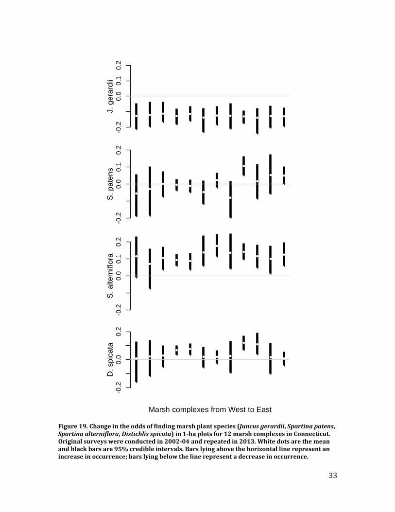
Figure 19. Change in the odds of finding marsh plant species (Juncus gerardii, Spartina patens, Spartina alterniflora, Distichlis spicata) in 1-ha plots for 12 marsh complexes in Connecticut. Original surveys were conducted in 2002-04 and repeated in 2013. White dots are the mean and black bars are 95% credible intervals. Bars lying above the horizontal line represent an increase in occurrence; bars lying below the line represent a decrease in occurrence.

-0.2

0.0

0.1

0.2

1

J.

gera

rdii

-0.2

0.0

0.1

0.2

1

S. p

ate

ns

-0.2

0.0

0.1

0.2

1

S. a

lte

rniflo

ra-0

.20

.00

.2

1

D. sp

icata

Marsh complexes from West to East

34

Figure 20. The change in Mean-High-Water (MHW) between marsh vegetation survey periods, with the contribution of the 18.6-year lunar cycle removed from the trend. The lunar cycle contribution that was removed is shown below.

Saltmarsh phenology Methods – The year prior to this project we established plots for the collection of data on the timing of leaf-out, flowering, and seed production for four dominant saltmarsh species (Spartina alterniflora, S. patens, Distichlis spicata, and Phragmites australis). Our initial plan was to continue this data collection during this study, but our pilot year experience suggested that our sampling was too small scale to be representative. Instead, in 2014 we conducted a second pilot study and deployed a “PlantCam” (http://www.wingscapes.com/wingscapes-timelapsecam) at Barn Island WMA from April to June to (1) test whether we could estimate tidal marsh “green-up” phenology using time-lapse photography, and (2) derive a green-up baseline for the site. We include that analysis here to augment the vegetation data that we have been collecting and to provide a “proof-of-concept” for this method of tracking phenology.

We mounted the PlantCam on the stem of a red cedar in the third impoundment, facing east so that high marsh, low marsh, panne habitat, and coastal forest were all in the frame. We used image analysis software to estimate the green-up trend throughout the spring. We used a section of high marsh habitat within the

1.4

1.6

1.8

MH

W (

Ma

y 1

- A

ug

ust 3

1)

m a

bo

ve M

SL

2002 2005 2008 2011-0

.06

-0.0

30.0

0

18

.6 y

r lu

nar

cycle

con

trib

utio

n (

m)

2002 2005 2008 2011

http://www.wingscapes.com/wingscapes-timelapsecam

35

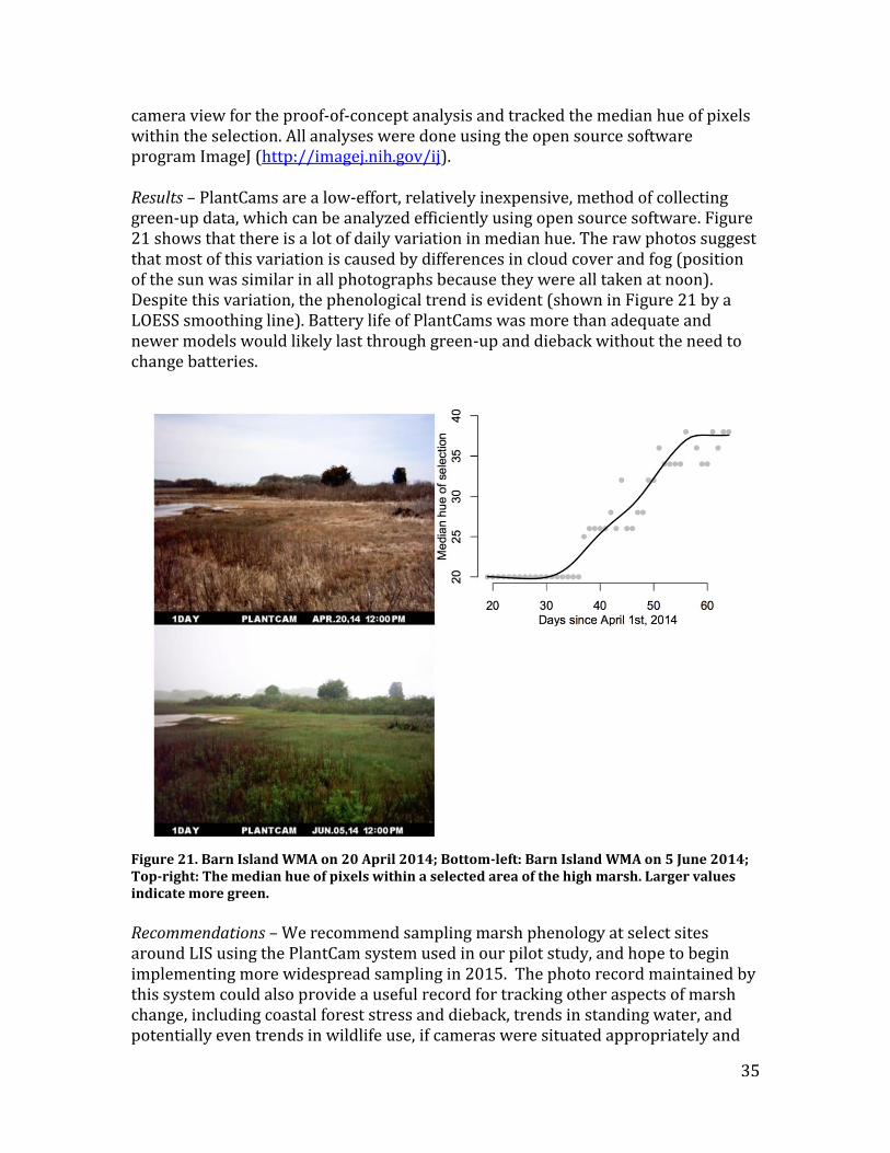
camera view for the proof-of-concept analysis and tracked the median hue of pixels within the selection. All analyses were done using the open source software program ImageJ (http://imagej.nih.gov/ij). Results – PlantCams are a low-effort, relatively inexpensive, method of collecting green-up data, which can be analyzed efficiently using open source software. Figure 21 shows that there is a lot of daily variation in median hue. The raw photos suggest that most of this variation is caused by differences in cloud cover and fog (position of the sun was similar in all photographs because they were all taken at noon). Despite this variation, the phenological trend is evident (shown in Figure 21 by a LOESS smoothing line). Battery life of PlantCams was more than adequate and newer models would likely last through green-up and dieback without the need to change batteries.

Figure 21. Barn Island WMA on 20 April 2014; Bottom-left: Barn Island WMA on 5 June 2014; Top-right: The median hue of pixels within a selected area of the high marsh. Larger values indicate more green.

Recommendations – We recommend sampling marsh phenology at select sites around LIS using the PlantCam system used in our pilot study, and hope to begin implementing more widespread sampling in 2015. The photo record maintained by this system could also provide a useful record for tracking other aspects of marsh change, including coastal forest stress and dieback, trends in standing water, and potentially even trends in wildlife use, if cameras were situated appropriately and

http://imagej.nih.gov/ij

36

implemented over the long term. Each camera costs approximately $150, including the cost of mounting equipment and batteries to run the unit for one year. Barn Island WMA would be an ideal place to set up photo stations to take advantage of existing historical photographs, but we envision a network of sites to capture LIS-wide patterns. Saltmarsh transgression Methods – Georeferenced aerial photos from http://magic.lib.uconn.edu and http://www.ct.gov/deep/cwp/view.asp?a=2698&q=322898&deepNav_GID=1707 did not have the resolution needed to detect potential forest dieback caused by increased saltwater inundation, which we expected to be a relatively small effect of perhaps just a few meters. Consequently, we used the raw image files to georeference photos from different years at an appropriate resolution. First, we created a grid with 1-ha squares covering all marshes in CT and randomly selected 200 squares. We then georeferenced the raw aerial images only to the extent of a given square (using separate images for each square), allowing us to significantly improve the precision and accuracy of the orthorectification procedure compared to existing aerial photos. We used only squares for which we could achieve a root mean square error (RMSE) of less than 0.5 m, meaning that any given point on the photo is likely within 1 m of its true location. RMSE was assessed using the Orthorectify tool in ArcGIS (ArcGIS Desktop: Release 10. Redlands, CA: Environmental Systems Research Institute). Photos for 27 plots met this requirement, on which we traced the total area of forest at three time steps: 1974, 1990, and 2010. Each plot and time step was traced 10 times non-consecutively by the same observer, and the resulting measurement error was explicitly incorporated into a hierarchical model that made it possible to estimate dieback with uncertainty bounds that include measurement error. Results – We found no evidence for an overall trend in forest dieback, and in some areas along the forest/marsh ecotone, there is even evidence of forest expansion (Figure 22). We think that forest increases are unlikely to be caused by forest transgressing into marsh, however. Instead it seems likely that we were measuring a larger canopy extent as a result of the forest maturing. This analysis could be biased by our requirement that RMSE be less than 0.5 m, which makes it likely that plots with boulders, docks, and other structures are overrepresented in our sample because these features were often required to cross-reference photographs accurately. Recommendations – Our results suggest that anecdotal reports of coastal forest dieback as a result of sea-level rise need to be considered in the larger geographic context: while trees may be dying back in some areas, there appear to be just as many areas where forest is continuing to mature with no signs of stress. This surprising pattern was reinforced by our estimates of tree growth rates at the marsh edge (see above). Rates of sea-level rise in LIS over the 36-year span of our aerial photo analysis were ~ 2 mm/year, yet we were not able to detect a forest

http://magic.lib.uconn.edu/

http://www.ct.gov/deep/cwp/view.asp?a=2698&q=322898&deepNav_GID=1707

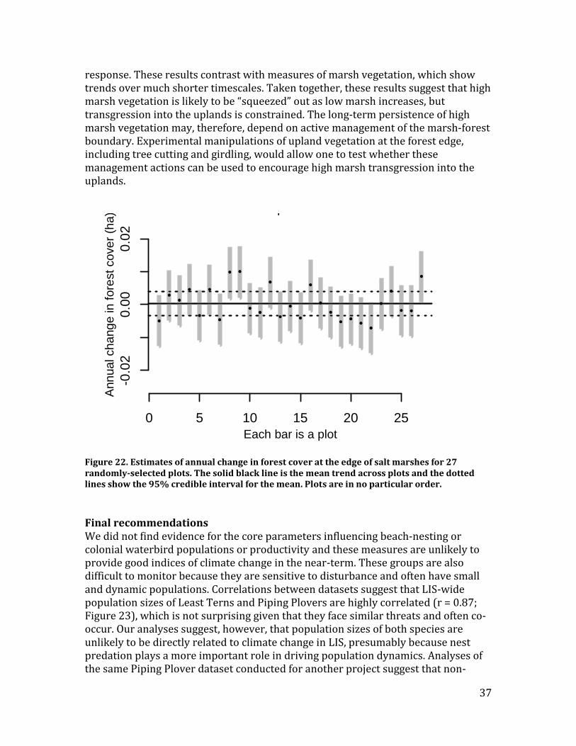
37

response. These results contrast with measures of marsh vegetation, which show trends over much shorter timescales. Taken together, these results suggest that high marsh vegetation is likely to be “squeezed” out as low marsh increases, but transgression into the uplands is constrained. The long-term persistence of high marsh vegetation may, therefore, depend on active management of the marsh-forest boundary. Experimental manipulations of upland vegetation at the forest edge, including tree cutting and girdling, would allow one to test whether these management actions can be used to encourage high marsh transgression into the uplands.

Figure 22. Estimates of annual change in forest cover at the edge of salt marshes for 27 randomly-selected plots. The solid black line is the mean trend across plots and the dotted lines show the 95% credible interval for the mean. Plots are in no particular order.

Final recommendations We did not find evidence for the core parameters influencing beach-nesting or colonial waterbird populations or productivity and these measures are unlikely to provide good indices of climate change in the near-term. These groups are also difficult to monitor because they are sensitive to disturbance and often have small and dynamic populations. Correlations between datasets suggest that LIS-wide population sizes of Least Terns and Piping Plovers are highly correlated (r = 0.87; Figure 23), which is not surprising given that they face similar threats and often co-occur. Our analyses suggest, however, that population sizes of both species are unlikely to be directly related to climate change in LIS, presumably because nest predation plays a more important role in driving population dynamics. Analyses of the same Piping Plover dataset conducted for another project suggest that non-

-2 -1 0 1 2

-5e-0

45

e-0

4

norm quantiles

Inte

rce

pts

-2 -1 0 1 2

-0.0

05

0.0

05

norm quantiles

Slo

pe

s

0 5 10 15 20 25

-0.0

20.0

00

.02

Each bar is a plot

Ann

ual ch

ang

e in

fore

st cove

r (h

a)

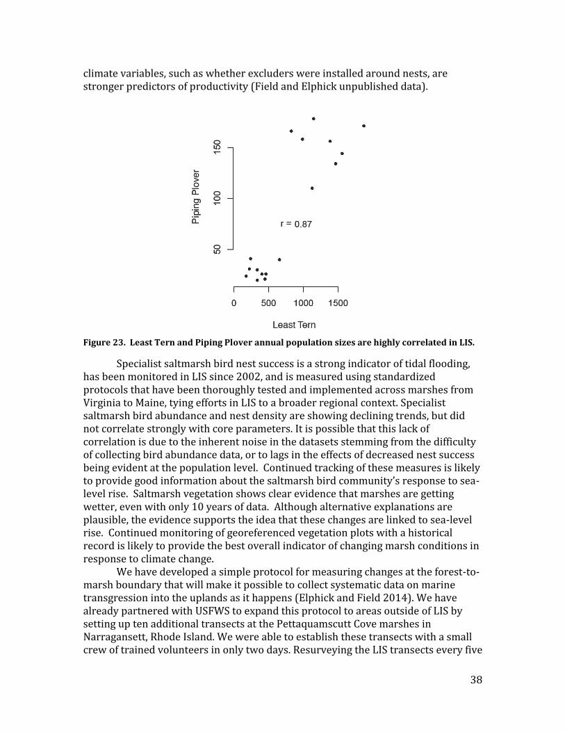
38

climate variables, such as whether excluders were installed around nests, are stronger predictors of productivity (Field and Elphick unpublished data).

Figure 23. Least Tern and Piping Plover annual population sizes are highly correlated in LIS.

Specialist saltmarsh bird nest success is a strong indicator of tidal flooding, has been monitored in LIS since 2002, and is measured using standardized protocols that have been thoroughly tested and implemented across marshes from Virginia to Maine, tying efforts in LIS to a broader regional context. Specialist saltmarsh bird abundance and nest density are showing declining trends, but did not correlate strongly with core parameters. It is possible that this lack of correlation is due to the inherent noise in the datasets stemming from the difficulty of collecting bird abundance data, or to lags in the effects of decreased nest success being evident at the population level. Continued tracking of these measures is likely to provide good information about the saltmarsh bird community’s response to sea-level rise. Saltmarsh vegetation shows clear evidence that marshes are getting wetter, even with only 10 years of data. Although alternative explanations are plausible, the evidence supports the idea that these changes are linked to sea-level rise. Continued monitoring of georeferenced vegetation plots with a historical record is likely to provide the best overall indicator of changing marsh conditions in response to climate change. We have developed a simple protocol for measuring changes at the forest-to-marsh boundary that will make it possible to collect systematic data on marine transgression into the uplands as it happens (Elphick and Field 2014). We have already partnered with USFWS to expand this protocol to areas outside of LIS by setting up ten additional transects at the Pettaquamscutt Cove marshes in Narragansett, Rhode Island. We were able to establish these transects with a small crew of trained volunteers in only two days. Resurveying the LIS transects every five

39

to ten years should be a high priority to begin quantifying rates of marine transgression across LIS. This is especially critical as our analyses of forest cover and growth rates at the forest-to-marsh boundary suggest that rates of transgression could be very low, while shifts from high marsh to low marsh vegetation appear to be happening quite rapidly. Tree cores, especially from oaks, at the marsh edge are a cost-effective method for monitoring changes over longer timescales and will likely provide the first indication that coastal forests are reaching a tipping point that would allow marine transgression to occur. Additional analysis efforts using the tree cores collected for this project, which we will archive in the international tree ring data bank (http://www.ncdc.noaa.gov/data-access/paleoclimatology-data/datasets/tree-ring), could extend the scope of inference beyond the 20 years examined here. Our results suggest that management experiments aimed at encouraging more rapid marine transgression should be a high priority because our results suggest that the natural rate of transgression will not be rapid enough to provide habitat in time to avoid the first extinctions of specialist saltmarsh fauna. Acknowledgments This work was primarily funded by a grant from the Connecticut Department of Energy and Environmental Protection/Long Island Sound Study. We also thank other sponsors of our work over past 12 years, as the data collected for those projects was integral to some of our current analyses: U.S. Environmental Protection Agency (Long Island Sound Study), National Oceanic and Atmospheric Administration (Connecticut Sea Grant), Connecticut Department of Environmental Protection (Wildlife Division, Office of Long Island Sound Programs), United States Fish and Wildlife Service, and the University of Connecticut (Ecology and Evolutionary Biology Bamford Fund). The project also would not have been possible without the cooperation and help of many other individuals and organizations. First, we thank the many Federal and state agencies, towns, land trusts, non-profit conservation organizations and private land owners who have given us access to their properties or provided other forms of assistance. Second, we thank Michael Whalen, Emma Young and the many UConn field assistants who have collected the body of data upon which this report is based. Third, we thank the many other researchers and citizen scientists who contributed information to the datasets that we have drawn on. Finally, this project arose from the Saltmarsh Habitat and Avian Research Program and we have benefited greatly from many lengthy discussions with our other collaborators in this long-term endeavor. References Barrett, J., J. Rose, S. Deonarine, A. Clemetson, J. Pagach, M. Parker, and M. Tedesco.

2011. Sentinel monitoring for climate change in the Long Island Sound estuarine and coastal ecosystems of New York and Connecticut. Available at: http://longislandsoundstudy.net/wp-content/uploads/2011/04/LIS_SMstrategy_v1.pdf

Bellard, C., C. Bertelsmeier, P. Leadley, W. Thuiller, and F. Courchamp. 2012 Impacts

http://www.ncdc.noaa.gov/data-access/paleoclimatology-data/datasets/tree-ring

http://www.ncdc.noaa.gov/data-access/paleoclimatology-data/datasets/tree-ring

http://longislandsoundstudy.net/wp-content/uploads/2011/04/LIS_SMstrategy_v1.pdf

http://longislandsoundstudy.net/wp-content/uploads/2011/04/LIS_SMstrategy_v1.pdf

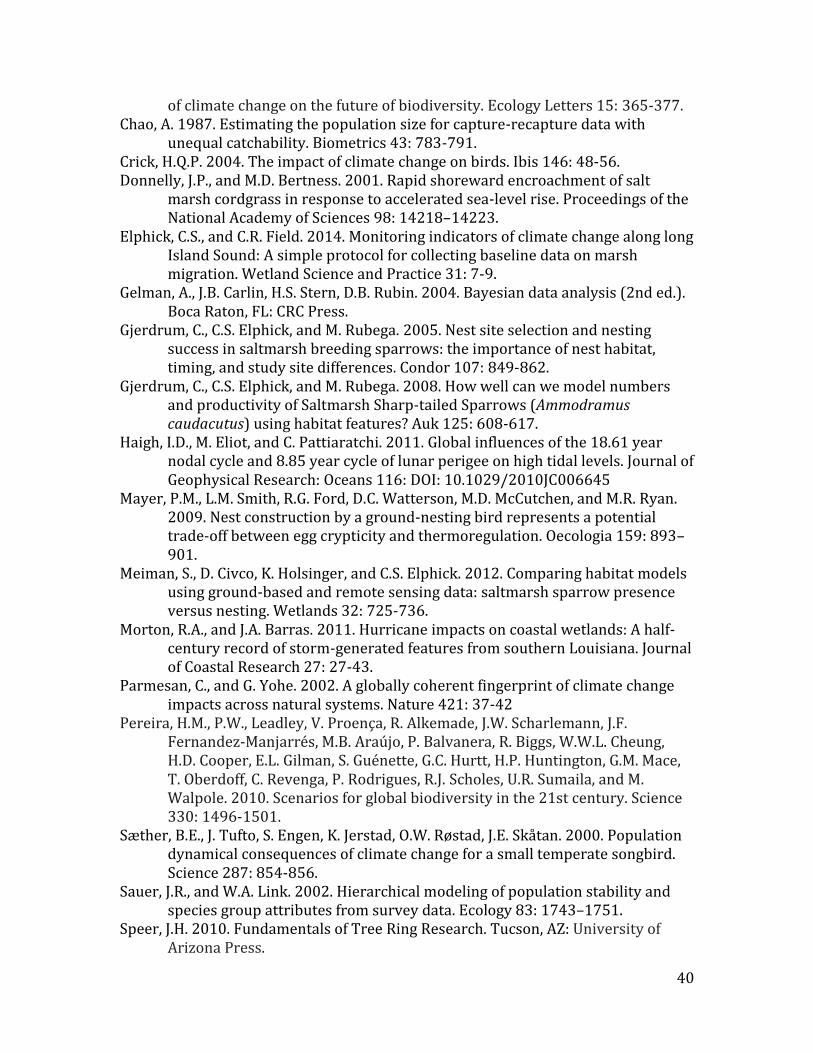
40

of climate change on the future of biodiversity. Ecology Letters 15: 365-377. Chao, A. 1987. Estimating the population size for capture-recapture data with

unequal catchability. Biometrics 43: 783-791. Crick, H.Q.P. 2004. The impact of climate change on birds. Ibis 146: 48-56. Donnelly, J.P., and M.D. Bertness. 2001. Rapid shoreward encroachment of salt

marsh cordgrass in response to accelerated sea-level rise. Proceedings of the National Academy of Sciences 98: 14218–14223.

Elphick, C.S., and C.R. Field. 2014. Monitoring indicators of climate change along long Island Sound: A simple protocol for collecting baseline data on marsh migration. Wetland Science and Practice 31: 7-9.

Gelman, A., J.B. Carlin, H.S. Stern, D.B. Rubin. 2004. Bayesian data analysis (2nd ed.). Boca Raton, FL: CRC Press.

Gjerdrum, C., C.S. Elphick, and M. Rubega. 2005. Nest site selection and nesting success in saltmarsh breeding sparrows: the importance of nest habitat, timing, and study site differences. Condor 107: 849-862.

Gjerdrum, C., C.S. Elphick, and M. Rubega. 2008. How well can we model numbers and productivity of Saltmarsh Sharp-tailed Sparrows (Ammodramus caudacutus) using habitat features? Auk 125: 608-617.

Haigh, I.D., M. Eliot, and C. Pattiaratchi. 2011. Global influences of the 18.61 year nodal cycle and 8.85 year cycle of lunar perigee on high tidal levels. Journal of Geophysical Research: Oceans 116: DOI: 10.1029/2010JC006645

Mayer, P.M., L.M. Smith, R.G. Ford, D.C. Watterson, M.D. McCutchen, and M.R. Ryan. 2009. Nest construction by a ground-nesting bird represents a potential trade-off between egg crypticity and thermoregulation. Oecologia 159: 893–901.

Meiman, S., D. Civco, K. Holsinger, and C.S. Elphick. 2012. Comparing habitat models using ground-based and remote sensing data: saltmarsh sparrow presence versus nesting. Wetlands 32: 725-736.

Morton, R.A., and J.A. Barras. 2011. Hurricane impacts on coastal wetlands: A half-century record of storm-generated features from southern Louisiana. Journal of Coastal Research 27: 27-43.

Parmesan, C., and G. Yohe. 2002. A globally coherent fingerprint of climate change impacts across natural systems. Nature 421: 37-42

Pereira, H.M., P.W., Leadley, V. Proença, R. Alkemade, J.W. Scharlemann, J.F. Fernandez-Manjarrés, M.B. Araújo, P. Balvanera, R. Biggs, W.W.L. Cheung, H.D. Cooper, E.L. Gilman, S. Guénette, G.C. Hurtt, H.P. Huntington, G.M. Mace, T. Oberdoff, C. Revenga, P. Rodrigues, R.J. Scholes, U.R. Sumaila, and M. Walpole. 2010. Scenarios for global biodiversity in the 21st century. Science 330: 1496-1501.

Sæther, B.E., J. Tufto, S. Engen, K. Jerstad, O.W. Røstad, J.E. Skåtan. 2000. Population dynamical consequences of climate change for a small temperate songbird. Science 287: 854-856.

Sauer, J.R., and W.A. Link. 2002. Hierarchical modeling of population stability and species group attributes from survey data. Ecology 83: 1743–1751.

Speer, J.H. 2010. Fundamentals of Tree Ring Research. Tucson, AZ: University of Arizona Press.

41

Thomas, C.D., and J.J. Lennon. 1999. Birds extend their ranges northwards. Nature 399: 213.

Thomas, C.D., A. Cameron, R.E. Green, M. Bakkenes, L.J., Beaumont, Y.C. Collingham, B.F.N, Erasmus, M.F.D, Siqueira, A. Grainger, and L. Hannah. 2004 Extinction risk from climate change. Nature 427:145-148.

Thrasher, B., J. Xiong, W. Wang, F. Melton, A. Michaelis, and R. Nemani. 2013. Downscaled climate projections suitable for resource management. Eos, Transactions American Geophysical Union 94: 321–323.

Walther, G.R., E. Post, P. Convey, A. Menzel, C. Parmesan, T.J.C. Beebee, J.M. Fromentin, O. Hoegh-Guldberg, and F. Bairlein. 2002. Ecological responses to recent climate change. Nature 416: 389-395.

Warren, R.S., W.A. Niering. 1993. Vegetation change on a northeast tidal marsh: Interaction of sea-level rise and marsh accretion. Ecology 74: 96–103.

Wong, K.C. 1990. Sea level variability in Long Island Sound. Estuaries 13: 362-372.

42

APPENDIX: Field Protocols Sentinels climate change monitoring: Identifying/georeferencing the marsh edge protocol (written by C. Field, January 2013; latest update Oct 2014) Each transect into the upland (see plot schematic) starts at a point located at the transition between salt marsh and upland vegetation. Identifying and creating a long-term record of this location with the greatest possible accuracy and precision is a top priority, as this information will be used to look for evidence of past marine transgression and will ensure that we have an accurate baseline that will allow us to make comparisons in the future. The first part of this protocol deals with identifying the marsh edge in the field, and the second part deals with georeferencing this location with the greatest possible accuracy and precision. Identifying the marsh edge We define the marsh edge according to vegetation because 1) we are primarily interested in monitoring how plant community composition changes across the transgression zone, and 2) it is likely that shifts in vegetation are the indicator of transgression that is most relevant to wildlife. We define the marsh edge as the seaward frontier of upland vegetation. For Long Island Sound, we define upland vegetation as any plant NOT listed in Table 1 of the Saltmarsh vegetation transects protocol. After navigating to your best estimate of where the point is located (accepting some error from the GPS unit), use the compass to identify the bearing of a transect that is perpendicular to the marsh edge. Record the bearing (relative to magnetic north) on the georeferencing datasheet. Within 2 m on either side of this transect, find the southern-most stem of upland vegetation. Place the flagged PVC on the transect line directly perpendicular to the identified stem and take a GPS reading (see below). Georeferencing the point The best strategy for georeferencing the point will depend on the GPS equipment being used. To be sure we can properly quantify the error in the estimated point coordinates, it is important to keep a record of what equipment is used and the details of the procedure on the georeferencing datasheet. All measurements should be taken in NAD83, UTM 18N. When using a Trimble w/ external antenna: Details will depend on 1) what software/routines are being used on the handheld computer to correct biases and increase precision, and 2) what post-processing will be used. Whatever combination of routines is used, it is important to attain sub-meter precision; sub-decimeter precision should be possible under most circumstances. One way to achieve this is to mount the external antenna in the PVC point marker and take a reading for at least 10 minutes.

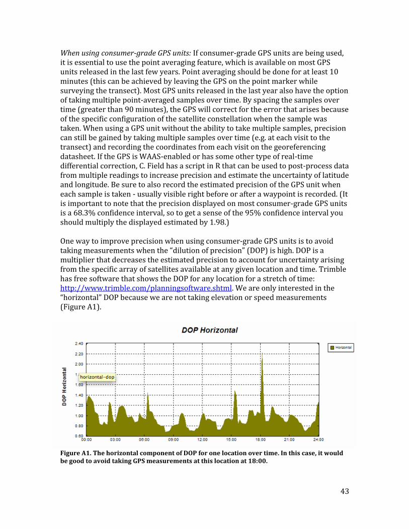
43

When using consumer-grade GPS units: If consumer-grade GPS units are being used, it is essential to use the point averaging feature, which is available on most GPS units released in the last few years. Point averaging should be done for at least 10 minutes (this can be achieved by leaving the GPS on the point marker while surveying the transect). Most GPS units released in the last year also have the option of taking multiple point-averaged samples over time. By spacing the samples over time (greater than 90 minutes), the GPS will correct for the error that arises because of the specific configuration of the satellite constellation when the sample was taken. When using a GPS unit without the ability to take multiple samples, precision can still be gained by taking multiple samples over time (e.g. at each visit to the transect) and recording the coordinates from each visit on the georeferencing datasheet. If the GPS is WAAS-enabled or has some other type of real-time differential correction, C. Field has a script in R that can be used to post-process data from multiple readings to increase precision and estimate the uncertainty of latitude and longitude. Be sure to also record the estimated precision of the GPS unit when each sample is taken - usually visible right before or after a waypoint is recorded. (It is important to note that the precision displayed on most consumer-grade GPS units is a 68.3% confidence interval, so to get a sense of the 95% confidence interval you should multiply the displayed estimated by 1.98.) One way to improve precision when using consumer-grade GPS units is to avoid taking measurements when the “dilution of precision” (DOP) is high. DOP is a multiplier that decreases the estimated precision to account for uncertainty arising from the specific array of satellites available at any given location and time. Trimble has free software that shows the DOP for any location for a stretch of time: http://www.trimble.com/planningsoftware.shtml. We are only interested in the “horizontal” DOP because we are not taking elevation or speed measurements (Figure A1).

Figure A1. The horizontal component of DOP for one location over time. In this case, it would be good to avoid taking GPS measurements at this location at 18:00.

http://www.trimble.com/planningsoftware.shtml

44

Sentinels climate change monitoring: Saltmarsh vegetation transects protocol (written by C. Field, February 2013; latest update Oct 2014) The purposes of this protocol are (1) to quantify the extent to which high marsh vegetation is present in the upland to look for evidence of marine transgression and (2) to create a baseline for future monitoring. The point of reference for this transect is the point that was marked and georeferenced and the bearing that was taken at the marsh edge according to the Identifying/georeferencing the marsh edge protocol. The saltmarsh vegetation transect protocol is based on two types of measurements which require a compass, measuring tape, and 1 m x 1 m plot square. Presence/absence in square plots Using the compass as a guide, roll out the measuring tape from the marsh edge point to 20 m in the direction of the transect bearing. Record the presence or absence of each high marsh or border species in each of 20 1 m x 1 m plots along the first 20 m of the transect (the center of each point will be at the half-meter mark - e.g. 0.5, 1.5, 2.5, etc.). Tables A1 and A2 have a list of all high marsh and border species likely to be found in Long Island Sound. Also survey two plots in the direction of the marsh (180 degrees from the transect bearing), with plots centered on -0.5 m and -1.5 m from the edge point. These are denoted as V00a and V00b (Distance = -1 and -2, respectively) on the data sheet. Record the presence of any high/low marsh or border species found within a 1 m x 1 m plot at 10 m intervals beyond the end of the original 20 m transect. Be sure to center the plot at each maker - e.g. centered on 30 m, 40 m, etc. Table A1. High or low marsh species likely to be encountered in Long Island Sound.

Common name Scientific name

Black grass Juncus gerardii

Salt grass Distichlis spicata

Salt hay grass Spartina patens

Saltmarsh cord grass Spartina alterniflora

Glasswort, pickleweed Salicornia spp.

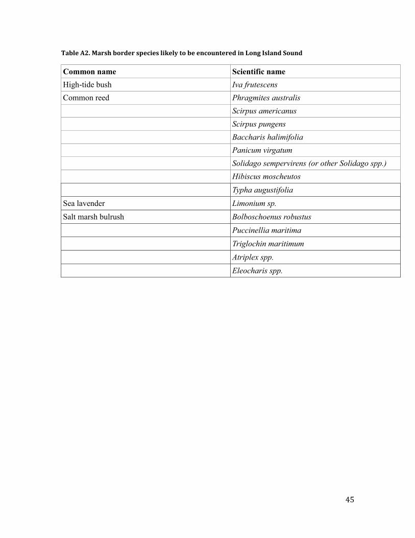
45

Table A2. Marsh border species likely to be encountered in Long Island Sound

Common name Scientific name

High-tide bush Iva frutescens

Common reed Phragmites australis

Scirpus americanus

Scirpus pungens

Baccharis halimifolia

Panicum virgatum

Solidago sempervirens (or other Solidago spp.)

Hibiscus moscheutos

Typha augustifolia

Sea lavender Limonium sp.

Salt marsh bulrush Bolboschoenus robustus

Puccinellia maritima

Triglochin maritimum

Atriplex spp.

Eleocharis spp.

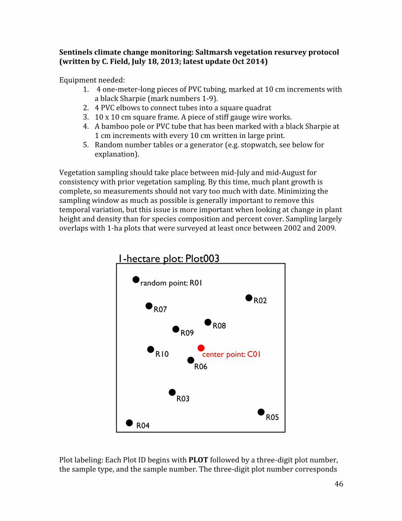
46

Sentinels climate change monitoring: Saltmarsh vegetation resurvey protocol (written by C. Field, July 18, 2013; latest update Oct 2014) Equipment needed:

1. 4 one-meter-long pieces of PVC tubing, marked at 10 cm increments with a black Sharpie (mark numbers 1-9).

2. 4 PVC elbows to connect tubes into a square quadrat 3. 10 x 10 cm square frame. A piece of stiff gauge wire works. 4. A bamboo pole or PVC tube that has been marked with a black Sharpie at

1 cm increments with every 10 cm written in large print. 5. Random number tables or a generator (e.g. stopwatch, see below for

explanation). Vegetation sampling should take place between mid-July and mid-August for consistency with prior vegetation sampling. By this time, much plant growth is complete, so measurements should not vary too much with date. Minimizing the sampling window as much as possible is generally important to remove this temporal variation, but this issue is more important when looking at change in plant height and density than for species composition and percent cover. Sampling largely overlaps with 1-ha plots that were surveyed at least once between 2002 and 2009.

Plot labeling: Each Plot ID begins with PLOT followed by a three-digit plot number, the sample type, and the sample number. The three-digit plot number corresponds

1-hectare plot: Plot003

center point: C01

random point: R01

R03

R02

R04R05

R06

R07

R08R09

R10

47

to the “universal plot number” used in previous years’ bird and plant surveys. The sample type denotes whether the sample is at a center point (C) of a historical 1-ha plot, a sample randomly selected from within the 1-ha plot (R), or at a point with a permanent marker (P; includes any plots done around abandoned sampling equipment, such as wooden stakes or PVC wells). The sample number is a two-digit number that provides unique identifiers to samples within a sample type, within a 1-ha plot. For example, the 14th random sample from within universal plot 3 should be recorded as PLOT003R14. In most cases, there will only be one sample labeled with a C for each 1-hectare plot, which should be labeled with the last three characters C01. If the sample is not located in a historical plot, record XXX for the plot number – e.g. PLOTXXXP01. The center point and permanent points should be surveyed using the full protocol outlined below (front and back of the data sheet). Random points should be surveyed using the streamlined set of measurements in green below (front of the data sheet only). Random points should be pre-loaded on a GPS unit, and care should be taken to get as close as possible to the point. If any portion of a random sample falls in a ditch, discard the point and select the next random point on the list. Do NOT just move the sample to one side of the ditch as doing this may bias sampling. Sampling should follow the order listed on the datasheet and outlined below to avoid disturbance to the vegetation that could bias subsequent measurements.

Locating the sampling frame

1. Place meter frame in any orientation such that target point lies at center of the

frame. When possible, all of the random samples within a 1-ha plot should be

done on the same day.

Vegetation cover measurement

2. Estimate the cover of major vegetation types as seen from above the sample. If

each plant species was a different color, and you were to take a high-resolution

picture of the sample from overhead, the percentage of pixels of each color is

what we are aiming to estimate. We are focusing on the plants listed on the data

sheet (including bare ground) such that values add to 100%: J. gerardii, S. patens,

D. spicata, S. alt short form, S. alt tall form, Salicornia sp., I. frutescens,

Limonium sp., P. australis, bare ground, wrack, and thatch. Note that we are

estimating the tall and short forms of S. alterniflora separately. Short form is less

than 14 inches tall. If a plant not listed on the datasheet is present and its coverage

is greater than 5%, you may add it to a blank slot on the datasheet. But, record

the percentage of all the major species on the datasheet, even if it is less than

5%. When a cover type is less than 1% (as can happen with Salicornia for

example), round up to 1%. Each species cover estimate should be broken out into

live vegetation and dead (but not thatch) vegetation. For example, if the sample

frame is 60% S. patens, 20% of which is dead (but not thatch), record 40% under

S. patens – alive and 20% under S. patens – dead. Be sure that the sum of all

48

cover types listed on the front page of the datasheet (which includes the live and

dead subcategories for each species) is 100%.

Thatch height

3. Measure the distance from the ground to the top of the thatch at the center point in

cm.

Bearing 4. Take the bearing along one side of the sample square to the nearest half-degree.

Be as accurate as possible.

Vegetation height measurement

5. Measure the height (in cm) and record the species of the tallest piece of vegetation

at each of the four corners of the frame. Be sure to follow the stem of the tallest

vegetation down to the mud and hold it flush against the measuring stick.

Vegetation density measurement

6. Generate 2-digit random numbers for the vegetation density measurements.

Ideally, this will have been done before going out into the field using an online

random number generator (this approach is best because it gives greater

confidence that the numbers truly are random). Random number generators are

also available as free smart phone apps, providing an in-field alternative. If these

options are unavailable, an alternative is to use the stopwatch or timer function on

a watch. One person should press the stop button at periodic intervals, yielding 2-

digit millisecond values. Be sure to write the random numbers in the appropriate

box on the datasheet.

7. Use these numbers to place the 10 x 10 cm frame for each vegetation density

measurement, using the southern-most corner of the square as the origin of an X-

Y plane. For example, for 26, go to the 2 (20 centimeter) mark on the PVC tube

that is along the X-axis and the 6 mark on the tube that is along the Y-axis. Place

the 10 cm frame where these values meet in the center of the quadrat. For a zero

or a nine, the small frame will lie against the edge of the meter frame, up against

the PVC.

8. Once the location for the density count has been established, count the number of

stems within the 10 x 10 cm frame for each of three groups: 1) J. gerardii, 2) S.

patens, and 3) all other species combined.

9. Repeat this process for five measures of stem density for each sample frame. If a

pair of random numbers is repeated within the five pairs selected, simply select

another pair of numbers.

Frequently asked questions What is thatch, and what is dead vegetation? Thatch is dead vegetation that is lying down, but rooted, that often (but not always) has live vegetation sticking up through it. When thatch is no longer rooted, it is wrack. The grass species (with the exception of P. australis) make thatch, although D. spicata most often has dead plants that are standing up, and thus have not yet become thatch. Dead Limonium, Salicornia, P. australis, and I. frutescens do not fit our definition of thatch, but dead plants should be noted in the comments, as described above. Sometimes in the tall S. alterniflora, the layer of thatch is very loose, so defining what constitutes thatch vs. dead plants

49

is difficult. In these cases, record thatch as the "main" layer that is lying down, and don't worry about the sticky-uppy stuff that protrudes above this horizontal layer. What do I record for thatch height if there is no real thatch layer? Zero. I’m doing a survey at high tide, and the live vegetation is covered by water. While standing water usually falls under the “bare” category, we ignore any water that covers live vegetation – just pretend it is not there. When possible, it is a good idea to avoid doing vegetation surveys during the highest tides. When doing the percent cover measurement, is it OK to part the grass to figure out which plants are dead, look for rare cover types I might be missing, and ID any ambiguous stems? Yes. Just be sure to follow the protocol outlined above once you have good idea of what is in the plot and are ready to take the percent cover measurement.

50

Sentinels climate change monitoring: Tree mortality protocol (written by C. Field, March 2013; latest update Oct 2014) The purpose of this protocol is to quantify the extent of crown dieback and tree mortality along a transect from the marsh edge into the forest. The point of reference for this transect is the point that was marked and georeferenced and the bearing that was taken at the marsh edge according to the Identifying/georeferencing the marsh edge protocol. The tree mortality transect protocol requires a 100 m measuring tape (metric), a compass, measuring tape, a two m measuring stick, diameter tape (metric), and a tree ID guide - Sibley's Guide to Trees is probably the best guide to use if you're an ornithologist. Setting up the transect Using the compass as a guide, roll out the measuring tape from the marsh edge point to the full length of the transect in the direction of the transect bearing. The full length of the transect is determined before going out into the field (you should aim for 75 – 100 m), but often it is impossible to go the full length before reaching a property line, wall, cliff, or trail. Transects should be at least 20 m long. For each tree > 1 cm diameter at breast height (dbh) within 1 m on either side of the transect line, take several measures: Distance Record how far along the transect each tree is, measuring the point along the transect that intersects with a perpendicular line from the center of the base of the tree. Distances should be recorded to the nearest cm - e.g. 14.05 m. Alive? Record a 1 if the tree has at least one leaf; 0 if there are no leaves. Broken? Record a 1 if a main stem of the tree is broken; 0 if there is no physical damage or only branches are broken. % dieback Percent crown dieback is a measure of current stresses on a tree. To measure dieback, we are following the procedures outlined in the Forest Inventory and Analysis (FIA) Program. First, identify the base of the “obvious live crown”. From the FIA protocol: “The "obvious live crown" is described as the point on the tree where most live

branches/twigs above that point are continuous and typical for a tree species (and/or tree

size) on a particular site. Include most crown branches/twigs, but exclude epicormic

twigs/sprigs and straggler branches that usually do not contribute much to the tree's

growth. The base of the live branch/twig bearing the lowest foliage may be above or

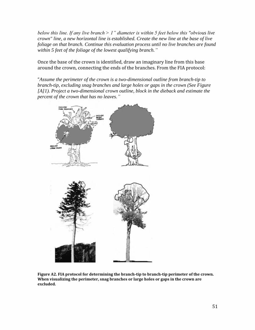
51

below this line. If any live branch > 1” diameter is within 5 feet below this "obvious live

crown" line, a new horizontal line is established. Create the new line at the base of live

foliage on that branch. Continue this evaluation process until no live branches are found

within 5 feet of the foliage of the lowest qualifying branch.” Once the base of the crown is identified, draw an imaginary line from this base around the crown, connecting the ends of the branches. From the FIA protocol: “Assume the perimeter of the crown is a two-dimensional outline from branch-tip to

branch-tip, excluding snag branches and large holes or gaps in the crown (See Figure

[A]1). Project a two-dimensional crown outline, block in the dieback and estimate the

percent of the crown that has no leaves.”

Figure A2. FIA protocol for determining the branch-tip to branch-tip perimeter of the crown. When visualizing the perimeter, snag branches or large holes or gaps in the crown are excluded.

52

Species Record the tree species. If you cannot determine species in the field, collect or take a picture of a leaf (on a whiteboard with the point and tree ID number) to bring back to the lab for identification. Diameter at breast height (dbh) Use the diameter tape to measure diameter of the stem at 1.3 m off the ground. If there are multiple stems at this height, measure and record the diameter of each stem. Sandy? If a tree is dead, is it likely a casualty of hurricane Sandy? 1 - Yes; 0 - No; M - Maybe; UK - unknown. If tree damage is suspected to be Sandy-related, it might be useful to take a picture to send to a manager later. Sandy how? If a 1, 0, or M, record how you made this determination. E.g. “Clearly fresh break, and in an area that is known to have been impacted by Sandy” or “Expert opinion from NAME”. Picture and core (Y/N) Was a picture taken for ID or to evaluate whether it was Sandy damage? Was a tree core taken to measure growth rings?

53

Sentinels climate change monitoring: Edge point count protocol (written by C. Field, April 2013; last update Oct 2014) The edge count should be conducted at the point that was marked at the marsh edge according to the Identifying/georeferencing the marsh edge protocol. The protocol for the count is based on the SHARP Callback Survey Protocol (http://www.tidalmarshbirds.net/?page_id=1595), but with several important modifications: For both Primary and Secondary Species, the distance bands are 0-25m, 25-50m (there is no >50m). For Primary Species, just follow the protocol outlined in the SHARP Callback Survey Protocol using the modified distance bands. For Secondary Species, follow the protocol outlined in the SHARP Callback Survey Protocol, but (1) we are tracking species, not individuals, and (2) we are not recording the distance band or the precise distance (the last column before comments on the datasheet). Because these details are being omitted, secondary species only need one line per species, with an X (rather than tick marks) if any individual of a species was detected in one of the 5 passive count minutes.

sentinels of climate change: coastal indicators of

Documents