seasonal cycle of cloud cover analyzed using meteosat · pdf fileseasonal cycle of cloud cover...

Seasonal cycle of cloud cover analyzed using Meteosat images

J. Massons1, D. Domingo1, J. Lorente2

1 Lab. FõÂ sica Aplicada, Univ. Rovira i Virgili. Pl. Imperial Tarraco 1, E-43005 Tarragona, Spain2Dept. Astronomia i Meteorologia. Univ. Barcelona. Avda. Diagonal 647, E-08028 Barcelona, Spain

Received: 8 October 1996 /Revised: 8 September 1997 /Accepted: 9 September 1997

Abstract. A cloud-detection method was used to re-trieve cloudy pixels from Meteosat images. High spatialresolution (one pixel), monthly averaged cloud-coverdistribution was obtained for a 1-year period. Theseasonal cycle of cloud amount was analyzed. Cloudparameters obtained include the total cloud amount andthe percentage of occurrence of clouds at three altitudes.Hourly variations of cloud cover are also analyzed.Cloud properties determined are coherent with thoseobtained in previous studies.

Key words. Cloud cover á Meteosat

1 Introduction

Clouds have a powerful in¯uence on the radiationbudget because they provide the greatest contribution tothe scattering of solar radiation, enhancing the albedo ofthe earth-atmosphere system. Randall et al. (1984)estimate that a 4% increase in global low-cloud fractioncould o�set a 2±3 K rise in global temperature due to adoubling of CO2. However, the full role of clouds incontrolling the current climate is still far from under-stood, and remains one of the main causes of uncer-tainty in climate modelling. In order better to usesatellite images for analyzing cloud distributions, manyworks have been devoted to cloud detection by sepa-rating the satellite observations into clear and cloudycategories (Saunders, 1986; Rossow and Garder, 1993).

Although the measurement of cloudiness poses manyproblems, the need to study clouds and predict themcorrectly is widely recognized. As pointed out by severalauthors (Slingo, 1987) the major problem in the valida-tion of cloudiness is the di�erence in de®nition betweenmodels and observations. Surface observations have

been compiled from many years of observation (Warrenet al., 1986, 1988). In recent years these data have beensupplemented by satellite observations, which providebetter global distribution and spatial resolution. Inaddition to providing poor spatial coverage, surfaceobservations cannot view the cloud top, which is thepart of the cloud re¯ecting solar radiation and emittingthermal radiation. Satellite radiometers view the cloudtops and are able to produce a global data set ofspatially averaged cloud parameters.

Following Rossow et al. (1985), there are severallimitations on the evaluation of the cloud amount usingsatellite data. Among them must be cited the limitationsin global uniformity and space and time resolution ofthe data and the lack of a ``truth'' data set against whichto compare the results of each algorithm in order tojudge the performance of each method. The advantagesof a cloud climatology derived from satellite data haveled to the implementation of important internationalprograms such as the International Satellite CloudClimatology Project (ISCCP) (Rossow and Schi�er,1991; Drake, 1993). ISCCP has created a global clima-tology by combining data collected by both geostation-ary and polar orbiting satellites. The data used in thisresearch span the years 1984±1990. The cloud-detectionprocess is discussed in detail in Rossow and Garder(1993). The pixel level results are averaged to an equal-area grid with spatial resolution of about 280 km toproduce cloud fraction and average cloud properties at3-h intervals. These data have been used to analyze thediurnal variation of cloudiness over large areas (Rossowand Schi�er, 1991; Kondragunta and Gruber, 1994;Rozendal et al., 1995). Ground-based observations ofclouds include classi®cation by morphology and baseheight above the local terrain (Warren et al., 1986,1988). Classi®cation made from satellite observationsuses the division of clouds by their top height and/oroptical thicknesses (Minnis and Harrison, 1984; Desboisand SeÁ ze, 1984; Pankiewicz, 1995; Massons et al., 1996).In the present paper the temporal and spatial variationsof cloud fractions are investigated using satellite data

Correspondence to: Dr. J. Massonse-mail: [email protected]

Ann. Geophysicae 16, 331±341 (1998) Ó EGS ± Springer-Verlag 1998

provided by Meteosat for one complete year. Theanalysis is performed at 12:00 GMT with a resolutionof one pixel (about 7 ´ 5 km). In recent years, greatattention has been paid to the analysis of the cycles ofcloud fraction, both seasonal and diurnal (Minnis andHarrison, 1984; Duvel and Kaudel, 1985; Warren et al.,1985; Rossow and Lacis, 1990; Rossow and Schi�er,1991; Thiao and Turpeinen, 1992; Drake, 1993; Carlstonand Wolf, 1993; Klein and Hartmann, 1993; Norris andLeovy, 1994). Most of them use ISCCP data averagedover large spatial regions or are restricted to only a shortperiod. Data available through ISCCP provide a highnumber of global cloud data whose full potential willtake time to be discovered. Unfortunately, this does notallow a pixel-scale spatial analysis; this requirement isessential for the study of small-scale cloud structuresand/or heterogeneous land areas, and demands acomplementary higher-resolution data base. There havebeen many assessments of the e�ect of image pixel sizeon cloud cover determination (see references in Rossowet al., 1985, 1993). So, for example, the analysis of sub-pixel-size clouds such as cumulus indicates (Rozendaalet al., 1995) that missing small cumulus clouds becauseof their spatial scale and small e�ects on thermalinfrared radiances will produce substantial errors inthe statistical analysis of the cloud ®eld.

The analysis of the satellite data is described inSect. 2. In particular it includes a brief description of thecloud-detection scheme used. As Rossow et al. (1985)pointed out, the largest di�erences between cloud-detection methods occur in areas where the surfaceproperties varied rapidly in time or over small spatialscales. Areas where a signi®cant portion of clouds wereeither very low level and broken or optically very thinalso require a speci®c treatment. In order to increase theaccuracy, all the algorithms should be made sensitive tothe presence of clouds in low contrast situations. So, inthe present study an algorithm based on the analysis ofspatial and time variations in the image was used. Themethod follows the work of Coakley and Bretherton(1982) which uses the local spatial variance to separatethe homogeneous regions from intermediate points,interpreted as a partially covered ®eld of view. TheCoakley and Bretherton method uses the general obser-vation that clear regions exhibit smaller spatial varia-tions than do broken cloud regions. This methodologywas also applied by Coakley and Baldwin (1984) foranalyzing fair-weather and trade-wind cumulus. Themain results obtained from the application of thealgorithm are presented in Sect. 3. They include com-parisons of the cloud amount obtained here and ISCCPdata, as well as a series of plots describing the seasonalvariation of the parameters analyzed.

2 Satellite data and preprocessing

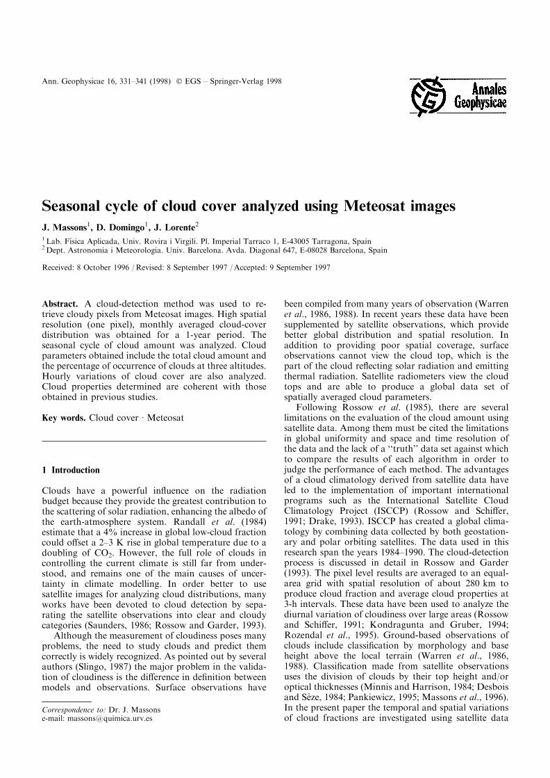
The images used in the present work correspond toMeteosat digital images. Images correspond to awindow region of 512 ´ 512 pixels centered on theIberian Peninsula and cover the domain shown in Fig. 1.

Visible (VIS) and thermal infrared (IR) images of 12:00GMT from August 1994 to July 1995 were analyzed.The e�ects on the radiance of satellite viewing angle andsolar illumination geometries were reduced using astandard Lambertian correction model, i.e., dividing allVIS counts in the image by the cosine of the solar zenithangle. Hereafter, VIS data will refer to the VIS correctedimage. The conversion from IR counts to radiance ismade using the coe�cients stored in the calibrationblock of the header. Radiance is then converted tobrightness temperature using the inverse of the Planckfunction. Working with temperatures, instead of IRcount numbers, has the advantage of avoiding changesdue to the variations of the thermal calibration param-eters. This allows images from di�erent days to beaccurately compared. Hereafter IR data will refer tobrightness temperature computed from IR grey level.

Two kinds of result will be presented here: monthlyaveraged time-evolution of percentage of occurrence ofclouds over selected areas of the image, and seasonallyaveraged cloud amount over the whole analyzed win-dow. For the ®rst, cloud amount was analyzed in somedetail at points of the line AB (see Fig. 1). This lineincludes sea areas and land points and is especiallyinteresting for analysis of the spatial and temporalvariability of the cloudiness. The analysis is particular-ized for the points a, b, and c. These points, located overthe AB line, correspond both to sea areas (one locatedover the Mediterranean and the another over theAtlantic) and land surfaces (over Spain). Seasonallyaveraged cloud data will not be presented in the shadedarea located in the northern part of the analyzedwindow (Fig. 1). Data at those high latitudes havesigni®cant errors due to the low sun elevation anglesduring a great part of the year.

Fig. 1. Schematic view of the analyzed area; symbols are explained inthe text

332 J. Massons et al.: Seasonal cycle of cloud cover analyzed using Meteosat images

In the ®rst step of the image processing, clouds wereisolated using a cloud-detection method. This methoduses bispectral VIS-IR histograms (SeÁ ze and Desbois,1987; SeÁ ze and Rossow, 1991) together with spatialvariance (Coakley and Bretherton, 1982) and short-termtime-series to detect cloudy pixels in the image. Asestablished by Rossow et al. (1985), the diversity ofconditions encountered on earth precludes the use ofany one method everywhere. A successful global cloudalgorithm must be situation independent and employ aseries of tests to retain ¯exibility. For this reason, thecloud-detection algorithm used here employs both spaceand time contrast tests as well as radiance thresholdmethods (both in IR and VIS images). The method usesthe VIS-IR image pair corresponding to the instant to beanalyzed and the image pair of the previous hour. Itmust be indicated that the time contrast test has beenfound more e�ective than the spatial variant. Summa-rizing, the method divides the image into eight geo-graphical areas (1±8, see Fig. 1) more or lesshomogeneous, and uses a temporal coherence functionbetween the VIS-IR images to be analyzed and those of1 h earlier. The ®rst step in the processing involves thecomputation of the time composite coherence functionbetween the VIS (and IR) image to be analyzed and theone corresponding to 1 h earlier. The temporal coher-ence function at pixel �i; j� for VIS images is de®ned as:

where the subscript 1 indicates values evaluated in theimage of the analyzed hour and subscript 2 refers to dataobtained from the images of 1 h earlier. Overbarsindicate spatial mean values computed averaging thegrey levels on a 3 ´ 3 window centered on the computedpixel. A similar calculation is realized for IR images.Both VIS and IR temporal coherence functions measurethe temporal variability of the pixel. If a pixel is clear inboth the present-time and 1-h-earlier images, these twocoe�cients show high values. If the pixel is cloudy in thepresent-time and/or in the previous image, a greatervariability is introduced, which produces lower values ofthe coherence functions. The pixels having a lowtemporal variability in both VIS and IR channels areused as applicants for clear pixels and are used to buildthe bidimensional VIS-IR histogram (H2D) for high-coherence pixels. Pixels having low temporal variabilityare not necessarily clear because static cloud clusters arealso detected by this operator. A new step in the processis needed in order to eliminate cloudy pixels from theH2D obtained (and add clear pixels not detected bythe ®rst calculation). However, it must be indicatedthat the time coherence ®lter runs acceptably well,mainly because it allows the elimination of almost allpartially covered pixels and broken clouds, which are

the most di�cult to be detected. As already indicated,not all clear pixels are found to have high coherencevalues, but using the present method only a represen-tative portion of clear pixel population is needed to runthe detection procedure. The following step in theprocessing involves the computation of H2D for eachone of the eight geographically homogeneous zones ofthe image. Only the points having a high VIS and IRcoherence are used. After that, the warmest and darkestclass in the H2D is located. Each pixel of the imagehaving a brightness temperature (or VIS grey level)greater than (or lower than) the elements of that class isconsidered clear. This step collects the clear pixels thathave not been detected in the ®rst step (temporalcoherence method). Several authors have noted thedi�culties of the cloud-detection process in coastlines(Desbois and SeÁ ze, 1984; Saunders, 1986). For thisreason, every point belonging to a three-pixels-widecoastline is analyzed again in more detail. If it isclassi®ed as cloudy, the algorithm computes the mostpopulated class in the 5 ´ 5 neighboring pixels (outsidethe coastline) and the current pixel is assigned to thisclass. On the other hand, if the pixel is initially classi®edas clear, then the label of the pixel is not modi®ed andno other calculations are realized with it. Finally, it mustbe indicated that pixels classi®ed as clear in the 1-h-earlier image and cloudy in the current image are tested

for being assigned to mixed or undecided pixels (theyusually correspond to broken clouds, edges of greatcloud formations, etc.). For these pixels, the variance ofthe VIS and IR data is computed using a 3 ´ 3 windowcentered on the pixel. If the variance in the VIS and orIR channel is greater than 20 units, the pixel is classi®edas mixed. Otherwise it remains in the cloudy class. Theproduction of a cloud mask for a typical pair of imagesrequires less than 40 s on a Pentium PC running at160 MHz. The more consuming time process is thecomputation of the time coherence (about 60%). Clouddetection performs well, not only at noon, but at otherhours of the day.

As an example, Fig. 2a shows the time-evolution of12:00 GMT VIS and IR data from August to December1994 for point b, located over Spain. Points labelled `0'correspond to pixels detected as clear, `2' indicatescloudy pixels and `1' represents mixed or undecidedpixels; these pixels were not clearly identi®ed as cloudyor cloud-free using the thresholds. As can be observed,the proportion of the last group is relatively small(about 7%). In this work this last group of pixels weretreated as cloudy. Note the presence of cloudy pixelswith VIS or IR data values closer to the onescorresponding to clear pixels. This similarity in grey

CO�i; j� �

P1k;j;m�ÿ1

VIS1�i� k; j� m� ÿ VIS1�i; j��

VIS2�i� k; j� m� ÿ VIS2�i; j��

��P1k;j;m�ÿ1

VIS1�i� k; j� m� ÿ VIS1�i; j�� 2 P1

k;j;m�ÿ1VIS2�i� k; j� m� ÿ VIS2�i; j�� 2s ;

J. Massons et al.: Seasonal cycle of cloud cover analyzed using Meteosat images 333

levels, which occurs in semitransparent high-level cloudsor low-level stratus, hinders the use of cloud-detectionalgorithms. Days with no data in Fig. 2 were days forwhich the image of 11:00 or 12:00 GMT were not in ourhourly image data base.

As an indicator of cloud-detection performance,these short-term time-series of VIS and IR values werenumerically treated in order to determine the thresholdsto be used as separators between cloudy and clear pixels.Analyzing the frequency histograms of the data in amedium-term series of 31 days (15 before and 15 afterthe analyzed day), a standard class separation methodwas used to detect the threshold separating cloud andclear pixels. The VIS and IR threshold levels determinedin this way are plotted in Fig. 2a as solid lines. So, therelative value of the VIS-IR data indicates whether thepixel is detected clear or cloudy by this time-evolutionmethod. Few disagreements between both assignments(method used and medium-term time-series analysis)were found, showing the power of the method. Thesedisagreements are labelled as `x'. The amount ofdisagreement is relatively small (about 2% of the total).This amount is even smaller over sea surfaces, where thegrey level of the clear pixels is more homogeneous. Thecloud-detection method requires few computer resourcesand little a priori information (only the 1-h-previousVIS-IR image pair).

A comparison of the satellite-retrieved cloudiness forAugust±December 1994 with surface observations forpoint b (see Fig. 1) are presented in Fig. 2b. Surfaceobservation data were supplied in okta code by theInstituto Nacional de MeteorologõÂ a, the national mete-orological service of Spain, and correspond to thesynoptic surface station of Zamora, Spain (stationnumber 81300, located at 41.30°N, 5.44°W). All cloud

data were measured at 12:00 GMT. The upper part ofthe ®gure also includes the class, determined by thecloud-detection algorithm. A general agreement betweensurface observations and satellite derived cloudiness canbe observed, but, as indicated by SeÁ ze et al. (1983), it isalmost impossible to make general statements about thelevel of agreement between surface and satellite obser-vations of cloud amounts, especially as the area overwhich the comparation was undertaken is relativelysmall and su�ers from rapidly changing weather. Also,the di�erent point of view of both observations and thedi�erent area cover make di�cult the direct comparisonbetween these data. As indicated by Henderson-Sellerset al. (1987), the area of vision of a surface observer is100 ´ 100 km. This fact produces signi®cant di�erencesbetween surface and (one pixel) satellite observationswhen the cloud ®eld is nonuniform. Table 1 summarizesthe preceding comparison. The number of occurrencesof every octa value is computed for each pixel label(clear/mixed/cloudy) both for low and total cloudiness.The results indicate that almost all of the cases that aredetermined as clear by the cloud-detection algorithmcorrespond to low okta measurements and that thehigher octa values are associated with cases seen ascloudy by the algorithm. Taking into account the abovementioned reasons, the agreement between surface andsatellite observations is considered reasonable.

3 Results obtained

In order to test the accuracy of the cloud-detectionprogram, the results provided by the program for totalcloud amount at 12:00 GMT were compared withISCCP C1 data obtained for the 7-year period 1984±1990. For each pixel and each month, the total cloudamount is computed as the fraction of days duringwhich the pixel is seen as cloudy by the cloud-detectionprogram. Cloud amount is expressed as a percentageand corresponds to a time-averaged cloud-cover fractionover the pixel. The comparison between yearly averagedISCCP data and the present data spatially averagedonto the ISCCP grid shows a general agreement betweenboth data sets. So, for example, the averaged RMS ofthe di�erences between total cloud amount in the gridpoints for March, July, and November are respectively8, 7, and 12 (over 100). These di�erences can beconsidered su�ciently low, taking into account that

Fig. 2. a Time-evolution of VIS and IR data for August±December1994 and for point b. The legend is explained in the text. b Surfaceobservations in oktas of the cloudiness for point b

Table 1. Number of occurrences of okta values (total and low-levelclouds) for each clear-mixed-cloudy situation for point b

Octas 0 1 2 3 4 5 6 7 8

totalClear pixels 17 12 10 3 3 0 1 2 0Mixed pixels 0 1 0 0 1 1 3 2 1Cloudy pixels 1 2 0 4 3 2 12 21 20

lowClear pixels 4 3 3 1 1 0 1 0 0Mixed pixels 1 2 1 0 2 1 0 0 0Cloudy pixels 2 2 0 3 5 13 10 12 9


the data correspond to di�erent years and the greattemporal and spatial variability of the cloud ®eld.

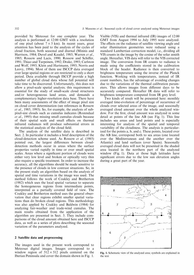
These two data ®elds are compared in more detailover the AB line (see Fig. 1). The cloud amountsdetermined for the AB line are depicted in Fig. 3 forJanuary, March, May, July, September, and November.ISCCP data are represented as solid lines (one line forevery year) and symbols are used to plot the cloud-amount data obtained here. In order to increase thelegibility of the plot, only one point is presented forevery 16 data values obtained (32 points for 512 datavalues). The plots show that the obtained cloud amountreproduces the behavior of the ISCCP data acceptably.This fact indicates that the cloud-amount data obtainedfor the time-period analyzed are representative of theclimatology of the area and that the cloud-detectionalgorithm correctly captures the threshold level separat-ing cloudy and cloud-free pixels. Cloud amount over theocean has a maintained behavior with cloud amount ofaround 70±80%, more or less independent of the season.Cloud amount over Spain is less (with cloud-amountdata ranging from 10±20% to 40±50%), with minimumvalues in winter and summer. Finally, cloud amountover the Mediterranean Sea is generally higher than overland, having pronounced minimum values during sum-mer months. Minor di�erences between ISCCP data andthe present data can be easily explained by the spatial

and temporal variability of the cloud-amount datadistribution, especially over land.

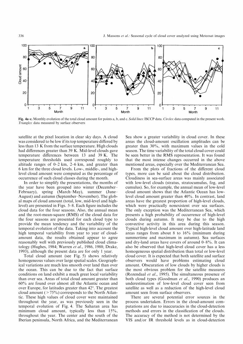
The monthly time-evolution of the cloud-cover datais presented in Fig. 4 for the three points a, b, and c(Fig. 1). ISCCP data for these points are also included.Again, the seasonal behavior of the obtained data agreesreasonably with ISCCP results. The data tendencyagrees with the preceding comments: high and main-tained cloud-amount values over points located on theocean, and more season-dependent values over theMediterranean Sea and (especially) over the land area.Strong gradients of percentage of occurrence of cloudscan be observed in the coastal areas, especially on theAtlantic coastlines. Cloud-amount values over Spain(point b), have been compared with okta values mea-sured by surface observers, provided by the NationalMeteorological Service of Spain and converted topercentage of cloud cover. The comparison showsdiscrepancies lower than 7% in average.

Global maps of cloud amount were obtained for theanalyzed window. The total cloud amount is the sum ofmean low-, middle-, and high-level cloud amount. Cloudlevel was determined from the di�erence between theequivalent black-body temperature of the surface and thetemperature of the cloud top (Minnis and Harrison,1984). For each pixel, surface temperature was computedas the monthly mean brightness temperature seen by the

Fig. 3a±f. Total cloud amount for the line section AB for di�erent months. a January, bMarch, cMay, d July, e September, f November. Solidlines: ISCCP data. Symbols: data computed in the present work


satellite at the pixel location in clear sky days. A cloudwas considered to be low if its top temperature di�ered byless than 13 K from the surface temperature. High cloudshad di�erences greater than 39 K. Mid-level clouds gavetemperature di�erences between 13 and 39 K. Thetemperature thresholds used correspond roughly toaltitude ranges of 0±2 km, 2±6 km, and greater than6 km for the three cloud levels. Low-, middle-, and high-level cloud amount were computed as the percentage ofoccurrence of such cloud classes during the month.

In order to simplify the presentations, the months ofthe year have been grouped into winter (December±February), spring (March±May), summer (June±August) and autumn (September±November). The glob-al maps of cloud amount (total, low, mid-level and high-level) are presented in Figs. 5±8. Each ®gure includes thecloud data for the four seasons. Also, the annual meanand the root-mean-square (RMS) of the cloud data forthe four seasons are presented for each cloud type toprovide the mean tendency and the variability of thetemporal evolution of the data. Taking into account thehigh temporal variability from year to year of cloud-amount data, the results obtained appear to agreereasonably well with previously published cloud clima-tology (Hughes, 1984; Warren et al., 1986, 1988; Drake,1993), although the present data are for only 1 year.

Total cloud amount (see Fig. 5) shows relativelyhomogeneous values over large spatial scales. Geograph-ical variations are much less smooth over land than overthe ocean. This can be due to the fact that surfaceconditions on land exhibit a much great local variabilitythan over sea. Areas of total cloud amount greater than60% are found over almost all the Atlantic ocean andover Europe, for latitudes greater than 42°. The greatestcloud amount (>75%) corresponds to the North Atlan-tic. These high values of cloud cover were maintainedthroughout the year, as was previously seen in thetemporal evolution of Fig. 4. The Saharan area hasminimum cloud amount, typically less than 15%,throughout the year. The center and the south of theIberian peninsula, North Africa, and the Mediterranean

Sea show a greater variability in cloud cover. In theseareas the cloud-amount oscillation amplitudes can begreater than 30%, with maximum values in the coldseason. The time variability of the total cloud cover couldbe seen better in the RMS representation. It was foundthat the most intense changes occurred in the abovementioned areas, especially over the Mediterranean Sea.

From the plots of fractions of the di�erent cloudtypes, more can be said about the cloud distribution.Cloudiness in sea-surface areas was mainly associatedwith low-level clouds (stratus, stratocumulus, fog, andcumulus). So, for example, the annual mean of low-levelcloud amount shows that the Atlantic Ocean has low-level cloud amount greater than 40%. In contrast, landareas have the greatest proportion of high-level clouds,which were practically nonexistent over sea surfaces.The only exception was the Mediterranean Sea, whichpresents a high probability of occurrence of high-levelclouds during autumn. It may be due to the highconvective activity in this area during this season.Typical high-level cloud amount over high-latitude landareas ranges from about 8 to 16% (minimum duringsummertime and maximum in autumn). Sea surfacesand dry-land areas have covers of around 0±8%. It canalso be observed that high-level cloud cover has a lesshomogeneous spatial distribution than total or low-levelcloud cover. It is expected that both satellite and surfaceobservers would have problems estimating cloudamount. Obscuration of low clouds by higher clouds isthe most obvious problem for the satellite measures(Rozendaal et al., 1995). The simultaneous presence ofboth cloud types (Goodman et al., 1990) produces anunderestimation of low-level cloud cover seen fromsatellite as well as a reduction of the high-level cloudamount seen from surface observers.

There are several potential error sources in theprocess undertaken. Errors in the cloud-amount com-putations are due to inaccuracies in the cloud-detectionmethods and errors in the classi®cation of the clouds.The accuracy of the method is not determined by theVIS and/or IR threshold levels as in cloud-detection

Fig. 4a±c.Monthly evolution of the total cloud amount for points a, b, and c.Solid lines: ISCCP data.Circles: data computed in the present work.Triangles: data measured by surface observers


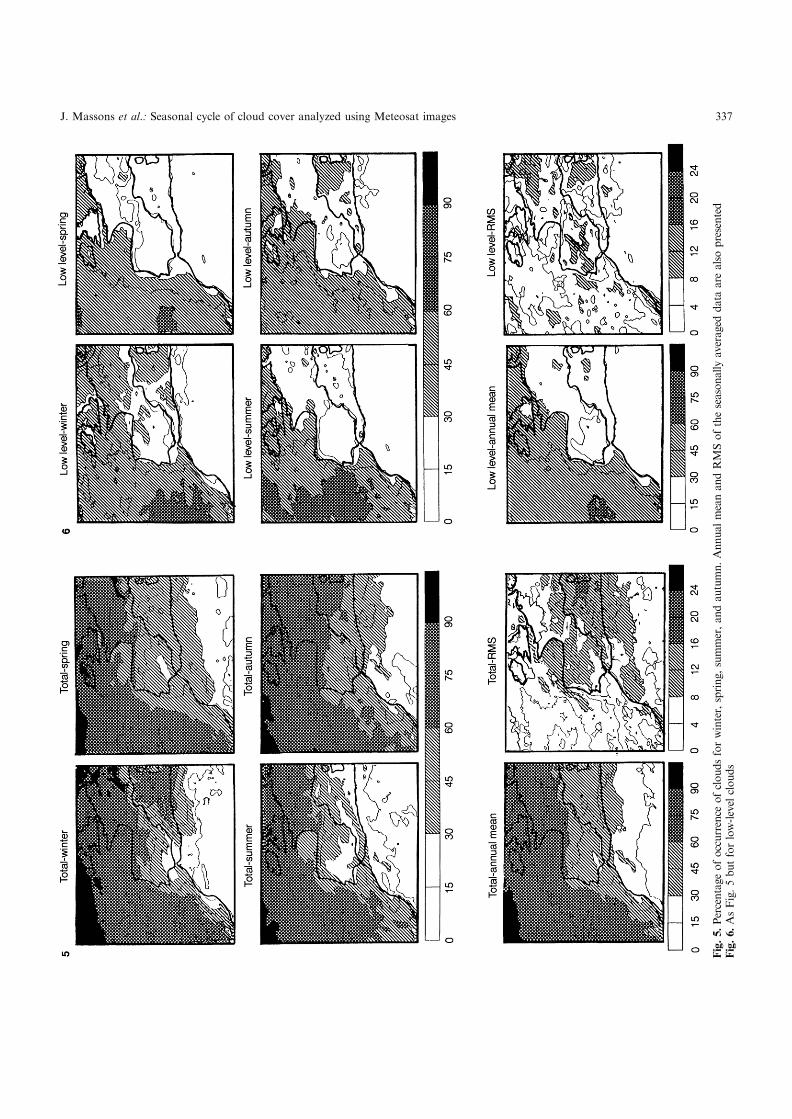
Fig.5.Percentage

ofoccurrence

ofcloudsforwinter,spring,summer,andautumn.AnnualmeanandRMSoftheseasonallyaveraged

dataarealso

presented

Fig.6.AsFig.5butforlow-levelclouds


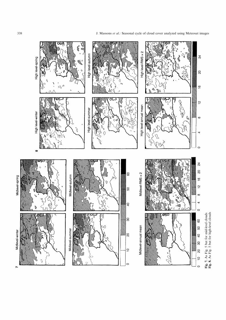
Fig.7.AsFig.5butformid-levelclouds

Fig.8.AsFig.5butforhigh-levelclouds


algorithms based on threshold techniques. Cloud-detec-tion errors are mainly produced in scenes where cloudscause few variations of the radiance. In other situations,even where cloudiness is usually persistent, the com-bined time-variation test and H2D histogram analysissuccessfully separate the radiance distribution into clearand cloudy categories. It should be noted that thealgorithm performs better over oceans than over land.In particular, complex situations over land, like snowcover during winter, are not correctly resolved by themethod. Even if a pixel is correctly classi®ed as cloudy,an additional error can occur in its classi®cation as low,mid-level or high-level cloud. The cloud-height calcula-tions are a�ected both by errors in the determinations ofthe surface temperature and the cloud-top temperature,mainly due to inaccuracies in the knowledge of theemissivity of the surface. Also, the uncertainties inthe vertical temperature gradient produce errors in theheight assignment.

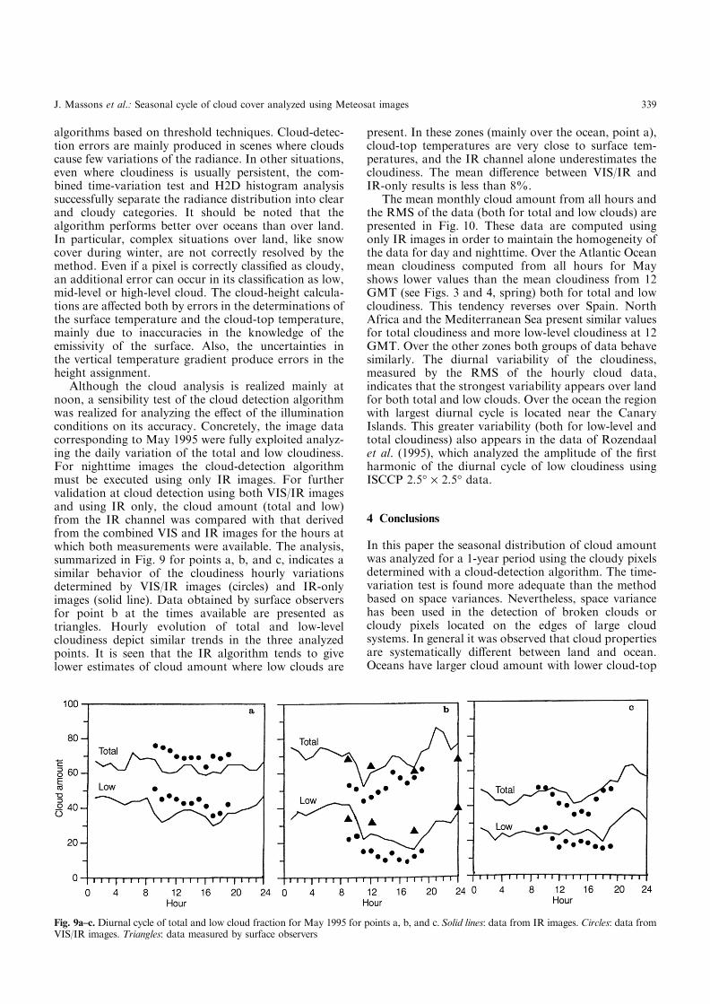
Although the cloud analysis is realized mainly atnoon, a sensibility test of the cloud detection algorithmwas realized for analyzing the e�ect of the illuminationconditions on its accuracy. Concretely, the image datacorresponding to May 1995 were fully exploited analyz-ing the daily variation of the total and low cloudiness.For nighttime images the cloud-detection algorithmmust be executed using only IR images. For furthervalidation at cloud detection using both VIS/IR imagesand using IR only, the cloud amount (total and low)from the IR channel was compared with that derivedfrom the combined VIS and IR images for the hours atwhich both measurements were available. The analysis,summarized in Fig. 9 for points a, b, and c, indicates asimilar behavior of the cloudiness hourly variationsdetermined by VIS/IR images (circles) and IR-onlyimages (solid line). Data obtained by surface observersfor point b at the times available are presented astriangles. Hourly evolution of total and low-levelcloudiness depict similar trends in the three analyzedpoints. It is seen that the IR algorithm tends to givelower estimates of cloud amount where low clouds are

present. In these zones (mainly over the ocean, point a),cloud-top temperatures are very close to surface tem-peratures, and the IR channel alone underestimates thecloudiness. The mean di�erence between VIS/IR andIR-only results is less than 8%.

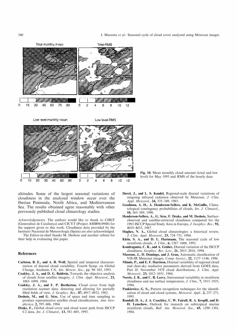
The mean monthly cloud amount from all hours andthe RMS of the data (both for total and low clouds) arepresented in Fig. 10. These data are computed usingonly IR images in order to maintain the homogeneity ofthe data for day and nighttime. Over the Atlantic Oceanmean cloudiness computed from all hours for Mayshows lower values than the mean cloudiness from 12GMT (see Figs. 3 and 4, spring) both for total and lowcloudiness. This tendency reverses over Spain. NorthAfrica and the Mediterranean Sea present similar valuesfor total cloudiness and more low-level cloudiness at 12GMT. Over the other zones both groups of data behavesimilarly. The diurnal variability of the cloudiness,measured by the RMS of the hourly cloud data,indicates that the strongest variability appears over landfor both total and low clouds. Over the ocean the regionwith largest diurnal cycle is located near the CanaryIslands. This greater variability (both for low-level andtotal cloudiness) also appears in the data of Rozendaalet al. (1995), which analyzed the amplitude of the ®rstharmonic of the diurnal cycle of low cloudiness usingISCCP 2.5° ´ 2.5° data.

4 Conclusions

In this paper the seasonal distribution of cloud amountwas analyzed for a 1-year period using the cloudy pixelsdetermined with a cloud-detection algorithm. The time-variation test is found more adequate than the methodbased on space variances. Nevertheless, space variancehas been used in the detection of broken clouds orcloudy pixels located on the edges of large cloudsystems. In general it was observed that cloud propertiesare systematically di�erent between land and ocean.Oceans have larger cloud amount with lower cloud-top

Fig. 9a±c. Diurnal cycle of total and low cloud fraction for May 1995 for points a, b, and c.Solid lines: data from IR images. Circles: data fromVIS/IR images. Triangles: data measured by surface observers


altitudes. Some of the largest seasonal variations ofcloudiness in the analyzed window occur over theIberian Peninsula, North Africa, and MediterraneanSea. The results obtained agree reasonably with otherpreviously published cloud climatology studies.

Acknowledgements. The authors would like to thank to CIRIT(Generalitat de Catalunya) and CICYT (Project AMB94-0948) forthe support given to this work. Cloudiness data provided by theInstituto Nacional de Meteorologia (Spain) are also acknowledged.

The Editor-in-chief thanks M. Desbois and another referee fortheir help in evaluating this paper.

References

Carlston, B. E., and A. B. Wolf, Spatial and temporal character-ization of diurnal cloud variability. Fourth Symp. on GlobalChange, Anaheim, CA, Am. Meteor. Soc., pp. 98±103, 1993.

Coakley, J. A., and D. G. Baldwin, Towards the objective analysisof clouds from satellite imagery, J. Clim. Appl. Meteorol., 23,1065±1099, 1984.

Coakley, J. A., and F. P. Bretherton, Cloud cover from highresolution scanner data: detecting and allowing for partially®lled ®elds of view, J. Geophys. Res., 87, 4917±4932, 1982.

Desbois, M., and G. SeÁ ze, Use of space and time sampling toproduce representative satellite cloud classi®cations, Ann. Geo-physica, 2, 595±606, 1984.

Drake, F., Global cloud cover and cloud water path from ISCCPC2 data, Int. J. Climatol., 13, 581±605, 1993.

Duvel, J., and L. S. Kaudel, Regional-scale diurnal variations ofoutgoing infrared radiation observed by Meteosat, J. Clim.Appl. Meteorol., 24, 335±349, 1985.

Goodman, A. H., A. Henderson-Sellers, and K. McGu�e, Clima-tological contingency probabilities of clouds, Int. J. Climatol.,10, 565±589, 1990.

Henderson-Sellers, A., G. SeÁ ze, F. Drake, and M. Desbois, Surface-observed and satellite-retrieved cloudiness compared for the1983 ISCCP Special Study Area in Europa, J. Geophys. Res., 92,4019±4033, 1987.

Hughes, N. A., Global cloud climatologies: a historical review,J. Clim. Appl. Meteorol., 23, 724±751, 1984.

Klein, S. A., and D. L. Hartmann, The seasonal cycle of lowstratiform clouds, J. Clim., 6, 1587±1606, 1993.

Kondragunta, C. R., and A. Gruber,Diurnal variation of the ISCCPcloudiness, Geophys. Res. Lett., 21, 2015±2018, 1994.

Massons, J., D. Domingo, and J. Grau, Automatic classi®cation ofVIS-IR Meteosat images, Comp. Geosci., 22, 1137±1146, 1996.

Minnis, P., and E. F. Harrison,Diurnal variability of regional cloudand clear-sky readiative parameters derived from GOES data.Part II: November 1978 cloud distributions, J. Clim. Appl.Meteorol., 23, 1012±1031, 1984.

Norris, J. R., and C. B. Leovy, Interannual variability in stratiformcloudiness and sea surface temperature, J. Clim., 7, 1915±1925,1994.

Pankiewicz, G. S., Pattern recognition techniques for the identi®-cation of cloud and cloud systems, Meteorol. Appl., 2, 257±271,1995.

Randall, D. A., J. A. Coackley, C. W. Fairall, R. A. Krop¯i, and D.H. Lenschow, Outlook for research on subtropical marinestratiform clouds, Bull. Am. Meteorol. Soc., 65, 1290±1301,1984.

Fig. 10. Mean monthly cloud amount (total and lowlevel) for May 1995 and RMS of the hourly data


Rossow, W. B., and L. C. Garder, Cloud detection using satellitemeasurements of infrared and visible radiances for ISCCP,J. Clim., 5, 2341±2369, 1993.

Rossow, W. B., and A. A. Lacis, Global, seasonal cloud variationsfrom satellite radiance measurements. Part II: properties andradiative e�ects, J. Clim., 3, 1204±1253, 1990.

Rossow, W. B., and R. A. Schi�er, ISCCP cloud data products,Bull. Am. Meteorol. Soc., 72, 2±20, 1991.

Rossow, W. B., F. Mosher, E. Kinsella, A. Arking, M. Desbois,E. Harrison, P. Minnis, E. Ruprecht, G. SeÁ zeÂ , C. Simmer, andE. Smith, ISCCP cloud algorithm intercomparison, J. Clim.Appl. Meteorol., 24, 877±903, 1985.

Rossow, W. B., A. W. Walker, and L. C. Garder, Comparison ofISCCP and other cloud amounts, J. Clim., 6, 2394±2418, 1993.

Rozendaal, M. A., C. B. Leovy, and S. A. Klein, An observationalstudy of diurnal variations of marine stratiform clouds, J. Clim.,8, 1795±1809, 1995.

Saunders, R. W., An automated scheme for removal of cloudcontamination from AVHRR radiances over western Europe,Int. J. Rem. Sensing, 7, 867±886, 1986.

SeÁ ze, G., and M. Desbois, Cloud cover analysis from satelliteimagery using spatial and temporal characteristics of the data,J. Appl. Meteorol., 26, 287±303, 1987.

SeÁ ze, G., and W. B. Rossow, Time cumulated visible and infraredradiance histograms used as descriptors of surface and cloudvariations, Int. J. Rem. Sensing, 12, 877±920, 1991.

(SeÁ ze et al. 1983)Slingo, J. M., The development and veri®cation of a cloud

prediction scheme for the ECMWF model, Q. J. R. Meteorol.Soc., 113, 899±927, 1987.

Thiao, W., and O. M. Turpeinen, Large-scale diurnal variations oftropical cold cloudiness based on a simple cloud indexingmethod, J. Clim., 5, 173±180, 1992.

Warren, S. G., C. J. Hann, and J. London, Simultaneousoccurrence of di�erent cloud types, J. Clim. Appl. Meteorol.,24, 658±667, 1985.

Warren, S. G., C. J. Hann, J. London, R. M. Chervin, and R. L.Jenne, Global distribution of total cloud cover and cloud typeamounts over land, NCAR/TN-273+STR, 1986.

Warren, S. G., C. J. Hann, J. London, R. M. Chervin, and R. L.Jenne, Global distribution of total cloud cover and cloudtype amounts over the ocean, NCAR/TN-317+STR, 1988.


seasonal cycle of cloud cover analyzed using meteosat · pdf fileseasonal cycle of cloud cover...

Documents