estimation of rainfall rates using 3d cloud ... - itc · properties from the meteosat second...
TRANSCRIPT

Estimation of Rainfall Rates Using 3D Cloud Properties from the Meteosat Second Generation and CloudSat Satellites
Edward L. Amoni March, 2010

Estimation of Rainfall Rates using 3D Cloud Properties from Meteosat Second Generation and CloudSat
Satellites
by
Edward L. Amoni Thesis submitted to the International Institute for Geo-information Science and Earth Observation in partial fulfilment of the requirements for the degree of Master of Science in Geo-information Science and Earth Observation, Specialisation: Advanced use of Remote Sensing in Water resource Management. Thesis Assessment Board Chairman Dr. Chris Mannaerts, WRS, ITC, Enschede External Examiner Dr. Rob Roebeling KNMI, De Bilt First Supervisor Prof. Bob (Z) Su WRS, ITC, Enschede Second Supervisor Ir. Joris Timmermanns WRS, ITC, Enschede
INTERNATIONAL INSTITUTE FOR GEO-INFORMATION SCIENCE AND EARTH OBSERVATION
ENSCHEDE, THE NETHERLANDS

Disclaimer This document describes work undertaken as part of a programme of study at the International Institute for Geo-information Science and Earth Observation. All views and opinions expressed therein remain the sole responsibility of the author, and do not necessarily represent those of the institute.

ESTIMATION OF RAINFALL RATES USING 3D PROPERTIES FROM THE METEOSAT SECOND GENERATION AND CLOUDSAT SATELLITES
1
Abstract
Availability of fresh water supply is essential to humans and all forms of life. Precipitation, being the source of most of fresh water plays an important role in the socio-economic activities as human settlement is often found in regions abundant with this precious commodity in its various forms either sourced directly from rainfall or from rivers, lakes, springs, etc. A good estimate of the amount of precipitation in any place assists the population in better planning of their activities that may include agriculture, infrastructure development and maintenance, flood and forest fire monitoring, etc. Several remote sensing based rainfall monitoring schemes are currently in existence. One of the best known is the Meteosat Second Generation, MSG’s Multi-sensor Precipitation Estimate (MPE). The MPE product relies mainly on the cloud top temperatures, a proxy for the cloud top-height, to estimate the rainfall intensity emanating from particular kinds of clouds with large vertical extent. The MSG has been useful in the estimation of rainfall intensity estimates especially for remote places over Africa and over the oceanic areas. On the other hand, as opposed to their counterparts in Western Europe, most of Africa is not covered by weather radar. This is attributed to affordability as these radars are costly. The weather radars have been known to give more accurate rainfall intensity estimates than the MSG, as demonstrated in Europe which is endowed with a network of weather radars under the OPERA network. An advantage of the radar technology is that it penetrates into the cloud to examine the properties of water and ice and considers them in estimation of rainfall intensities. The CloudSat satellite was introduced into orbit by NASA on 26 April 2006 as polar-orbiting experimental satellite. It applies active radar to penetrate the cloud and analyze its internal cloud properties. This satellite radar technology can be used to improve on the rainfall intensity estimation especially for those countries that are yet to acquire ground radar technology. However, being polar orbiting, the satellite also has its limitations, one which is its poor temporal resolution with a return cycle of between 14 – 16 days. Nevertheless, a synergetic use of the CloudSat and MSG products can be used to enhance the accuracy of rainfall forecasts. In this study, data from different clouds in several countries of Western Europe during the summer season was used, due to their advantage of having a network of weather radars under the OPERA system. Different cloud classes were tested, and the results showed that some properties of the clouds, namely the cloud ice water path (IWP), ice water content (IWC) and ice effective radius are important in the confirmation rainfall clouds. The thresholds were computed as IWP ≥ 38 gmˉ², IWC≥ 5.6
mgmˉ³ and ice effective radius ≥ 4.2 µm to sufficiently classify a cloud as a “rainy” cloud. The methodology was tested for the case of the Ewaso Nyiro catchment in the Kenya. The thresholds were tested for one rainy day, 24 October 2006, where hypothesis was confirmed.

ESTIMATION OF RAINFALL RATES USING 3D PROPERTIES FROM THE METEOSAT SECOND GENERATION AND CLOUDSAT SATELLITES
2
Acknowledgements
First and foremost I give thanks to God the Almighty for seeing me through this MSc Course. I also take this opportunity to thank my sponsor, the Netherlands Fellowship Programme (NFP), for providing me with this opportunity to study at the ITC. My appreciation goes to my employer, the Kenya Government through the Kenya Meteorological Department for giving me this chance to fulfil my dream of acquiring an MSc Course in Remote Sensing and Water Resources Management. My greatest gratitude goes to my first supervisor, Prof Bob (Z) Su, for his useful comments and advises that encouraged me during the entire period of my pursuance of the thesis. To my second supervisor, Ir. Joris Timmermans, I appreciate the tremendous support you gave towards me in the accomplishment of my work especially during our many weekly progress meetings. Great thanks to the WREM staff especially Dr. Ben H. P. Maathuis for his advice, and Dr. Chris Mannaerts and PhD student, Ms. Jennifer Kinoti for their assistance in my data acquisition. Great thanks to my WREM 2009 classmates, especially Amos, Emmanuel, Marijani, Chenai and Donald. To the others that I may have not mentioned by name, credit goes to them for their continuous support and friendship during the entire duration of our study in the Netherlands. Special thanks to all friends whom we shared good company during the 18- month stay in Enschede. To my fellow Kenyans, I am glad to say that I had the most pleasant time with you all. To my family, my dear wife Lucy and our two sons Cedric and Eugene, I really appreciated your patience and prayers for my success and good health while I was away. To my parents, brothers and sisters, and all other members of the extended family, your support was not in vain.

ESTIMATION OF RAINFALL RATES USING 3D PROPERTIES FROM THE METEOSAT SECOND GENERATION AND CLOUDSAT SATELLITES
3
Table of contents
1. INTRODUCTION ......................................................................................................................... 8
1.1. BACKGROUND AND JUSTIFICATION ......................................................................................... 9
1.2. RESEARCH PROBLEM ............................................................................................................... 9
1.3. RESEARCH OBJECTIVE ........................................................................................................... 11
1.4. RESEARCH QUESTIONS .......................................................................................................... 12
1.5. RESEARCH HYPOTHESIS ........................................................................................................ 12
1.6. STUDY AREA .......................................................................................................................... 12
1.7. SATELLITES ............................................................................................................................ 13
1.7.1. CloudSat ........................................................................................................................ 13
1.7.2. MSG ............................................................................................................................... 13
2. THEORY ...................................................................................................................................... 15
2.1. THE RAINFALL FROM GROUND RADAR ................................................................................. 15
2.1.1. Reflectivity: .................................................................................................................... 15
2.1.2. The range and power of radar ....................................................................................... 17
2.1.3. Doppler radar ................................................................................................................ 17
2.1.4. Interpreting radar imagery ............................................................................................ 18
2.1.5. Causes of Error ............................................................................................................. 18
2.1.6. Advantages and Disadvantages of the Weather Radar ................................................. 19
2.2. DETAILED CLOUDSAT ALGORITHMS ..................................................................................... 20
2.2.1. Ice Water Algorithm ...................................................................................................... 20
2.2.2. Forward model and measurements ............................................................................... 20
2.2.3. The physics behind......................................................................................................... 20
2.2.4. Liquid water algorithm .................................................................................................. 21
2.2.5. Departures from lognormal distribution ....................................................................... 23
2.3. RETRIEVAL BY OPTICAL REMOTE SENSING SENSORS ........................................................... 24
2.3.1. Overview ........................................................................................................................ 24
2.3.2. Algorithm Description ................................................................................................... 24
2.3.3. Estimation of instantaneous rain rates .......................................................................... 24
3. MATERIALS AND METHODS ................................................................................................ 25
3.1. CLOUD TYPES ........................................................................................................................ 27
3.2. MSG DATA ............................................................................................................................ 27
3.3. CLOUDSAT DATA ................................................................................................................... 28
3.4. RETRIEVAL BY GROUND RADAR SENSORS ............................................................................ 29
3.4.1. Ground radar ................................................................................................................. 30
3.5. ASSUMPTIONS ........................................................................................................................ 32
4. RESULTS ..................................................................................................................................... 34
4.1. DENSE AND DRIZZLE CLOUDS ............................................................................................... 34
4.1.1. Case 1: Dense cloud in Belgium.................................................................................... 34
4.1.2. Case 2: Drizzle cloud in S. West Netherlands ............................................................... 36

ESTIMATION OF RAINFALL RATES USING 3D PROPERTIES FROM THE METEOSAT SECOND GENERATION AND CLOUDSAT SATELLITES
4
4.1.3. Case 3: Drizzle cloud: N.E Netherlands and E. Germany ............................................ 36
4.1.4. Case 4: Drizzle cloud over W. Germany, 10 June 2009 ............................................... 37
4.2. PRECIPITATING CLOUDS ........................................................................................................ 37
4.2.1. Case 1: United Kingdom, 27 May 2007 ........................................................................ 37
4.2.2. Case 2: Southern France, 31 May 2007 ........................................................................ 40
4.2.3. Case 3: Northern France, 9 May 2007 .......................................................................... 40
4.2.4. Case 4: South Eastern Netherlands, 7 June 2009 ......................................................... 42
4.3. NON - PRECIPITATING CLOUDS .............................................................................................. 44
4.3.1. Case 1: S.W. Netherlands, 10 March 2009 ................................................................... 44
4.3.2. Case 2: Western Germany, 7 June 2009, 12:45 UTC ................................................... 44
4.3.3. Case 3: Northern Netherlands 1 June 2009 at 02:10 UTC ........................................... 45
4.3.4. Case 4: Eastern Netherlands 7 June 2009 .................................................................... 45
4.4. STATISTICAL ANALYSIS ......................................................................................................... 48
5. DISCUSSION ............................................................................................................................... 51
5.1. CLOUD ICE AND RAIN THRESHOLDS ...................................................................................... 51
5.2. SOURCES OF ERROR ............................................................................................................... 51
5.2.1. Parallax ......................................................................................................................... 51
5.2.2. Time Difference ............................................................................................................. 52
5.2.3. Diverging Liquid Water Measurements......................................................................... 52
5.2.4. Inadequate Tropical Data.............................................................................................. 52
6. CONCLUSION AND OUTLOOK ............................................................................................. 53
6.1. RESEARCH QUESTIONS .......................................................................................................... 53
6.2. RESEARCH HYPOTHESIS ......................................................................................................... 53
6.3. CONCLUSION .......................................................................................................................... 54
6.4. OUTLOOK ............................................................................................................................... 54
REFERENCES ...................................................................................................................................... 55
APPENDIX 1:ILWIS STUFF ................................................................................................................... 58
APPENDIX 2: MAP PROJECTIONS ....................................................................................................... 58
APPENDIX 3: FORMAT OVERVIEW OF CLOUDSAT DATA PRODUCTS ................................................. 59
APPENDIX 4: BATCH ALGORITHM...................................................................................................... 62
APPENDIX 5: EWASO NYIRO (KENYA) DATA .................................................................................... 63

ESTIMATION OF RAINFALL RATES USING 3D PROPERTIES FROM THE METEOSAT SECOND GENERATION AND CLOUDSAT SATELLITES
5
List of figures
Figure 1-1: Simplified Hydrological cycle (Source: University of Nebraska-Lincoln, USA) ................ 9
Figure 1-2: CloudSat Cloud Profiling Radar (CPR) operational geometry. ........................................ 13
Figure 2-1: Sample of resultant map on ILWIS, after using the formula that converts reflectivity to rainfall intensity .................................................................................................................................... 17
Figure 3-1: Computer screen snapshot of the data retrieval using the HDF View .............................. 27
Figure 3-2: A screen-shot of MPE product of MSG indication areas of varying rainfall intensities. . 28
Figure 3-3: Image of the vertical cross-section of a CloudRadar Data (NASA) .................................. 29
Figure 3-4: Data from the Opera Network. In the left panel, the backscatter radar image is shown, for 31 May 2007, 13:00 UTC from the OPERA radar Network, (source KNMI). In the right panel, the retrieved rain rates are shown for 31 May 2007, 13:00 UTC. ............................................................. 31
Figure 3-5: Flow chart of methodology ................................................................................................ 32
Figure 4-1: Graph above showing the variation between ice water path and ice effective radius. ..... 35
Figure 4-2: Variation of the mean Ice effective radius per bin with the number of cloudy bins in the profile .................................................................................................................................................... 35
Figure 4-3: Graph showing the relationship between the mean RE and the mean IWC in a cloud during CloudSat overpass in N.E Netherland and W. Germany on 15 May 2009 at 12:40 UTC. ........ 37
Figure 4-4: Graph showing the direct relationship between the IWP and the Number of Cloudy bins38
Figure 4-5: Graph showing the variation between the mean ice water content and the resultant rainfall intensity. ................................................................................................................................... 39
Figure 4-6:Graph showing the variation between the MSG rainfall rates and those of the Radar Radar ..................................................................................................................................................... 39
Figure 4-7: Graph depicting direct relationship between mean ice effective radius within a profile with the corresponding number of icy bins. .......................................................................................... 40
Fig 4-8: Graph showing the relationship between the number of icy bins and the ice water content of the cloud within the CloudSat profiles. ................................................................................................. 41
Figure 4-9: Doppler radar backscatter image for the clouds on 7 June 2009, 12:45 UTC over the Netherlands, Belgium and Germany. .................................................................................................... 42
Figure 4-10: Doppler radar rainfall rate for the 7 June 2009, at 12:45 UTC ..................................... 42
Figure 4-11: Variation of vertical cloud ice water content with the rainfall rates for a cloud over South Eastern Netherlands on 7 June 2009 at about 12:45 UTC ......................................................... 43
Figure 4-12: Graph depicting the variation of the radar rainfall intensity with the cloud mean ice water content for the case of average value conditions for various cloud samples over Western Europe. .................................................................................................................................................. 46
Figure 4-13: Graph depicting the linear relationship between the ice effective radius and the radar rainfall for a clouds under mean conditions ......................................................................................... 47
Figure 4-14:Graph showing the relationship between the Ice water path and the Radar rainfall intensity for the on the average for the various clouds ......................................................................... 47
Figure 4-15: Summary of the MSG and radar rainfall rates comparison for all the study sites.......... 48
Figure 4-16: Flow chart of radar rain algorithm ................................................................................. 49

ESTIMATION OF RAINFALL RATES USING 3D PROPERTIES FROM THE METEOSAT SECOND GENERATION AND CLOUDSAT SATELLITES
6
List of tables
Table 4-1: Summary of the different internal cloud properties of a dense, non–precipitating cloud by CloudSat over Belgium on 4 May 2009. ................................................................................................ 34
Table 4-2: Light rain cloud, South West Netherlands, 13 May 2009, 1250 UTC ................................. 36
Table 4-3: Summary of internal cloud properties from CloudSat on a cloud over N.E Netherlands and W. Germany on 15 May 2009 at about 12:40 UTC. .............................................................................. 36
Table 4-4: Summary table of internal cloud properties of a drizzle cloud over West of Germany on 10 June 2009 at about 02:05 UTC ............................................................................................................. 37
Table 4-5: Summary of cloud properties from CloudSat during a rainy episode over the United Kingdom on 27 May 2007...................................................................................................................... 38
Table 4-6: Summary of the internal cloud properties from CloudSat over Southern France, 31 May 2007. ...................................................................................................................................................... 40
Table 4-7: Summary of the internal cloud properties from CloudSat over Northern France, 9 May 2007 ....................................................................................................................................................... 41
Table 4-8: Summary of internal cloud properties for a cloud over South Eastern Netherlands, 7 June 2009, 12:45 UTC ................................................................................................................................... 43
Table 4-9: Summary of internal cloud properties for a cloud over S.W Netherlands .......................... 44
Table 4-10: Summary of internal cloud properties for a cloud over W Germany ................................ 44
Table 4-11: Summary of internal cloud properties for a cloud over N. Netherlands ........................... 45
4-12: Summary of internal cloud properties for a cloud over Eastern Netherlands ............................ 45
Table 4-13: Summary of table of mean values of cloud properties against corresponding rainfall rates ............................................................................................................................................................... 46
Table 4-14: Summary for the threshold values of cloud internal ice properties with rainfall rates .... 47
Table 0-1: Summary of the Image Projection used for the KNMI radar image.................................... 58
Table 0-2: Summary of table of max value of cloud Properties against corresponding rainfall rates 68
Table 0-3: Summary of table of min value of cloud Properties against corresponding rainfall rates . 69

ESTIMATION OF RAINFALL RATES USING 3D PROPERTIES FROM THE METEOSAT SECOND GENERATION AND CLOUDSAT SATELLITES
7
Nomenclature
AFWA Air Force Weather Agency
CPR Cloud Profiling Radar
CloudSat Cloud Satellite mission operated by NASA
CDP Co-located Data Point
CWC Combined Water Content
DMSP Defence Meteorological Satellite Program DSD Drop Size Distribution
EBBT Equivalent Black body Brightness Temperatures ESA European Space Agency
ESSP Earth System Science Pathfinder
EUMETNET Network of European Meteorological Services
EUMETSAT European Organization for the Exploitation of Meteorological Satellites
FoV Field of View
HDF5 Hierarchical Data Format 5
K Kelvin
ILWIS Integrated Land and Water Information System
IPCC Intergovernmental Panel on Climate Change
IWC Ice Water Content
IWP Ice Water Path
KNMI Royal Netherlands Meteorological Institute (Koninklijk Nederlands Meteorologisch Instituut)
LUTs Look Up Tables
LWC Liquid Water Content
LWP Liquid Water Path
MPEF Meteorological Products Extraction Facility
MSG Meteosat Second Generation
MPE Multi-sensor Precipitation Estimate
OPERA Operational Programme on the Exchange of Weather Radar Information
NASA National Aeronautics and Space Administration
NWP Numerical Weather Prediction
PBs Processing Boxes
QPE Quantitative Precipitation Estimates
RADAR RAdio Detection And Ranging
SEVIRI Spinning Enhanced Visible and Infrared Imager
SSM/I Special Sensor Microwave Imager TRMM Tropical Rainfall Measuring Mission
UTC Universal Time Coordinate
VPR Vertical Profile of Reflectivity


ESTIMATION OF RAINFALL RATES USING 3D PROPERTIES FROM THE METEOSAT SECOND GENERATION AND CLOUDSAT SATELLITES
8
1. Introduction
Clouds play an important role in the water cycle of the Earth. Water continually moves between oceans, atmosphere, cryosphere and land. The properties and motion of the coherent cloud features are primarily determined by large-scale atmospheric circulations, which are pertinent manifestation of the weather systems (Menzel, 2001). The amount of water moved through the atmosphere in the hydrologic cycle per year is equivalent to the amount of water uniformly distributed over the surface of Earth with a depth of 1m. This amount of water annually enters the atmosphere through evaporation and returns to the surface as precipitation (Hartmann, 1994). In this cycle, clouds are the medium through which the transport takes place. Accurate information on cloud properties and their spatial and temporal variations are vital to studies regarding climate. Clouds regulate the energy balance between the ground and atmosphere by use of solar and thermal radiation (Cess et al., 1989). Despite the important role clouds play in the overall climate and weather forecast models, in most simulations they are characterized too simple resulting in large uncertainties in these models. This has led to the Intergovernmental Panel on Climate Change (IPCC) to call for more detailed quantification of cloud properties (IPCC., 2001), in order to have more accurate climate prediction models. Studies show that the radiative behaviour of clouds relies mainly upon the cloud physical properties like optical thickness, thermodynamic phase and droplet effective radius. Various methods have been developed to retrieve cloud optical thickness and effective radius using satellite radiances at wavelengths in the non-absorbing visible and moderately absorbing infra-red part of the electromagnetic spectrum (Nakajima et al., 1990). In addition to the climate impacts of clouds, they also directly influence many organisms on the earth, through precipitation. Areas perceived to have adequate precipitation are characterized by high population of both plant and animal species. This is caused by the many benefits of available water resulting from abundant rainfall. Measurements of rainfall have improved many aspects of human life, through the incorporation of rainfall rates and rainfall amount in atmospheric studies, development in water supplies, agriculture, transport (air and water), run-off (for hydroelectric power generation). It has become vital that more accurate measurements of rainfall amounts and rates need to be known, due to the ever increasing demand for precipitation water by the various sectors of the economy. This information of rainfall (rates and amount) should be made available to the end users within the shortest time possible. Meeting this demand requires the establishment of meteorological stations that represent the rainfall characteristics of every local area. As this is difficult to achieve with in-situ measurements most countries of Western Europe and Northern America have managed to establish a fairly good meteorological network.

ESTIMATION OF RAINFALL RATES USING 3D PROPERTIES FROM THE METEOSAT SECOND GENERATION AND CLOUDSAT SATELLITES
9
Figure 1-1: Simplified Hydrological cycle (Source: University of Nebraska-Lincoln, USA)
1.1. Background and Justification
Climatological data is vital in projects like road and bridge construction, dam construction, and even tourism expeditions. In many cases, this data may be unavailable because it was never recorded in the first place. In the years 2007 and 2008, many parts of the Southern Africa experienced one of their worst droughts in history, while Eastern Africa had one of their most severe floods to date. This resulted in bridges and roads being damaged by raging floods as a result of abnormally heavy rainfall. One of the reasons for this massive destruction of infrastructure was caused by flawed design. In their design the construction engineers implemented low thresholds for the endurance of the structures. These thresholds are supposed to be derived from historical data. In the case of absent historical data proxy data needs to be used, which tends to be subjective and therefore possess big error margins. If this data had been had been available the destruction of the infrastructure could had been greatly reduced. Despite the essential role that clouds play , good information on clouds is not everywhere available (Rossow et al., 1999). Vast lands are still unrepresented (although the number of operational networks for rainfall data is growing (especially over Europe and North America). This is because it is costly to establish a single fully fledged meteorological station together with associated infrastructure. In addition, meteorological equipment are general unique in design expensive and prone to periodic break-down, due to the effects of the environment. Quantitative Precipitation Estimates (QPE) both on high spatial and temporal resolution is vital in water management and Numerical Weather Prediction (NWP) studies for the meteorological and related fields.
1.2. Research Problem
Precipitation, is characterized by high spatial and temporal variation, yet is one of critical inputs for hydrological modelling. It is also an important factor influencing agriculture, water resources and ecosystems. Accurate measurements and prediction of precipitation are, therefore, are very important
for all rainfall-related applications (Wang et al., 2007). In reality many cases, weather forecasts have
ESTIMATION OF RAINFALL RATES USING 3D PROPERTIES FROM THE METEOSAT SECOND GENERATION AND CLOUDSAT SATELLITES
10
ended up being inaccurate to the disappointment of members of the public and other interested parties. It is believed that this is mainly due to the effect of clouds that are yet to be correctly represented in weather prediction models. Clouds play an important role of bringing water from the air, back to the ground. Their other important function is the important role they play in the earth’s solar and thermal radiation energy budget. In fact small changes in the cloud cover significantly alter the weather of any particular day. In spite of this, there has been lack of sufficient observational data to fully understand the properties and dynamics of the clouds, factors which can be important inputs in the weather prediction models. Generally speaking, rain gauge observations yield relatively accurate point measurements of precipitation, but they may suffer from sampling error in representing areal means, and also, they are absent in oceanic and sparsely populated land areas (Xie et al., 1995).In many areas of the developing world, especially in Africa, there is lack of precipitation data due to poor meteorological station network. This is mainly caused by high cost of running the weather stations, making them a non-priority for many developing countries. Rain gauges have over the years been used to physically measure daily rainfall accumulation at a point (~324 cm²) and have been providing fairly good quality data valid for small areas. These point measurements have been used in all kinds of hydrological models (Jayakrishnan et al., 2004). However, inconveniences caused with gauge rainfall measurements were documented in several studies (Legates et al., 1993). Another problem gauge networks is that they are vulnerable to poor levels of accuracy with increased rainfall intensities of flood producing storms. In general, rain gauge networks are not capable of detecting precipitation at the resolution and extent necessary for most hydrometeorology application. Errors caused by this inadequate gauge representation of precipitation fields are usually enhanced in runoff predictions (Finnerty et al., 1997). It is such challenges that make it prudent for the development of new approaches in the estimation of rainfall intensities. Most sectors of an economy require rainfall data for adequate planning. However, existing methods of estimating of rainfall amounts and rates are in most cases erroneous due to the fact that the present algorithms fail to capture the properties inside the clouds and details of the water and ice content from the vertical extent of the cloud. The current algorithms can be divided into 2 groups: infrared, microwave and radar.
• Infrared techniques which depend on cloud-top temperatures have a tendency of underestimating rainfall emanating from relatively warm clouds, and also often give misleading rainfall estimates for certain anvil and thick cirrus clouds with cold IR brightness temperature properties. The Spinning Enhanced Visible and Infra Red Imager (SEVIRI) which is on board the Meteosat Second Generation (MSG) satellite, is good at detecting back-scattered radiation from cloud tops in terms of brightness temperature. Since the atmospheric temperatures reduce with increasing altitude, cloud top are used to denote high clouds. In some cases, these cold clouds give an indication of precipitation although this is not always the case.

ESTIMATION OF RAINFALL RATES USING 3D PROPERTIES FROM THE METEOSAT SECOND GENERATION AND CLOUDSAT SATELLITES
11
• Microwave sensors and precipitation radar are the other tools that have recently gained popularity in this field, with the potential to improve precipitation estimates from the surface and from space. Microwave retrievals over the ocean are thought to rival radar retrievals for accuracy, but retrievals over land are compromised because of variations of the surface emissivity (Kummerow et al., 2001). Unlike IR, these techniques directly sense precipitation particles of water and ice rather than cloud top temperatures. Despite this, significant difficulties still remain. By use of infrared and visible techniques, satellite screening often detect many clouds because of cirrus which obscures lower clouds.
A new satellite-based cloud experiment, named the Cloud Satellite mission (CloudSat) was launched under the National Aeronautics Space Administration (NASA’s) Earth System Science Pathfinder (ESSP) programme in 2006 to assist in the quantification of the water and ice in clouds. It was the first space-borne millimetre wavelength radar. It is expected that data from CloudSat will fill the void that are currently inherent in the existing climate models. Scientists have good information from satellites regarding radiant energy distribution at the top of the atmosphere. However, little is known about how this energy is distributed within the atmosphere. CloudSat utilizes a special radar system to probe the cloud cover, and give information regarding the thickness of the cloud-layer, altitude of base and top layers, ice and water content within the clouds amongst other parameters that it measures. The unique feature of the radar lies in its ability to observe jointly most of the cloud condensate and precipitation within its nadir fields of view and its ability to provide profiles of these properties with a vertical resolution of 240 metres (Stephens et al., 2002). However, the most notable shortcoming of the CloudSat is its poor temporal resolution. The satellite’s revisit time at the equator is 16 days. On the other hand, MSG has better temporal resolution of 15 minutes. It is for this reason that images from both satellites will be used in unison to complement each other. Both the vertical extent of a cloud and its cloud top height may give an indication of the type of cloud, therefore enabling the designation of higher rainfall rates for deeper clouds and lower rainfall rates for shallower clouds. In the past, it was only the properties of the cloud tops that were used to determine the cloud characteristics, running the risk of designating rainfall to high-cold cirrus clouds with no potential for precipitation; and assigning of low rainfall to warm stratus-like clouds that are capable of precipitating.
1.3. Research Objective
The main objective of the study is the estimation of rainfall rates combining aspects of two satellites MSG’s SEVIRI and CloudSat. The specific objectives of the study are:
• To create a simple algorithm with the ability to estimates of rainfall rates with both aspects namely, high spatial resolution and high temporal resolution.
• Make use of the CloudSat to calibrate the SEVIRI Cloud top temperature (10.8µm band).

ESTIMATION OF RAINFALL RATES USING 3D PROPERTIES FROM THE METEOSAT SECOND GENERATION AND CLOUDSAT SATELLITES
12
• Estimate the rainfall rates for Europe, and then to compare the developed algorithm with the existing ones applicable for Africa in order to compensate for the vast areas which are currently un-gauged.
• To determine the type of cloud and therefore the probability of rainfall events.
1.4. Research Questions
• How can the rainfall estimates be improved by merging high temporal resolution Remote Sensing data from MSG with high spatial resolution Remote Sensing data from CloudSat?
• How can vertical profile information from CloudSat be merged with integrated profile information from SEVIRI?
• How do the sensor specifications (viewing angle, pixel size) influence the resultant rainfall rates?
1.5. Research Hypothesis
The study set the following Hypothesis: • Rainfall occurrence can be determined from the internal properties of clouds. • Ice particle characteristics within clouds are an important factor in determination of rainfall
intensity.
1.6. Study Area
The study area is the Western part of Europe within 35° N to 65° N latitude and 10°W and 20° E longitude. The area is preferred in the study due to its data reliability and good network of meteorological data. Most of the area in Northern and Central Europe receive good amounts of rainfall throughout the year with the exception of some areas, e.g. Spain in the Southern Europe part which is mainly of semi-arid nature.
Fig 2: Map of the countries of Western Europe (designed by Gecan/Waterfall HUM)
ESTIMATION OF RAINFALL RATES USING 3D PROPERTIES FROM THE METEOSAT SECOND GENERATION AND CLOUDSAT SATELLITES
13
1.7. Satellites
1.7.1. CloudSat
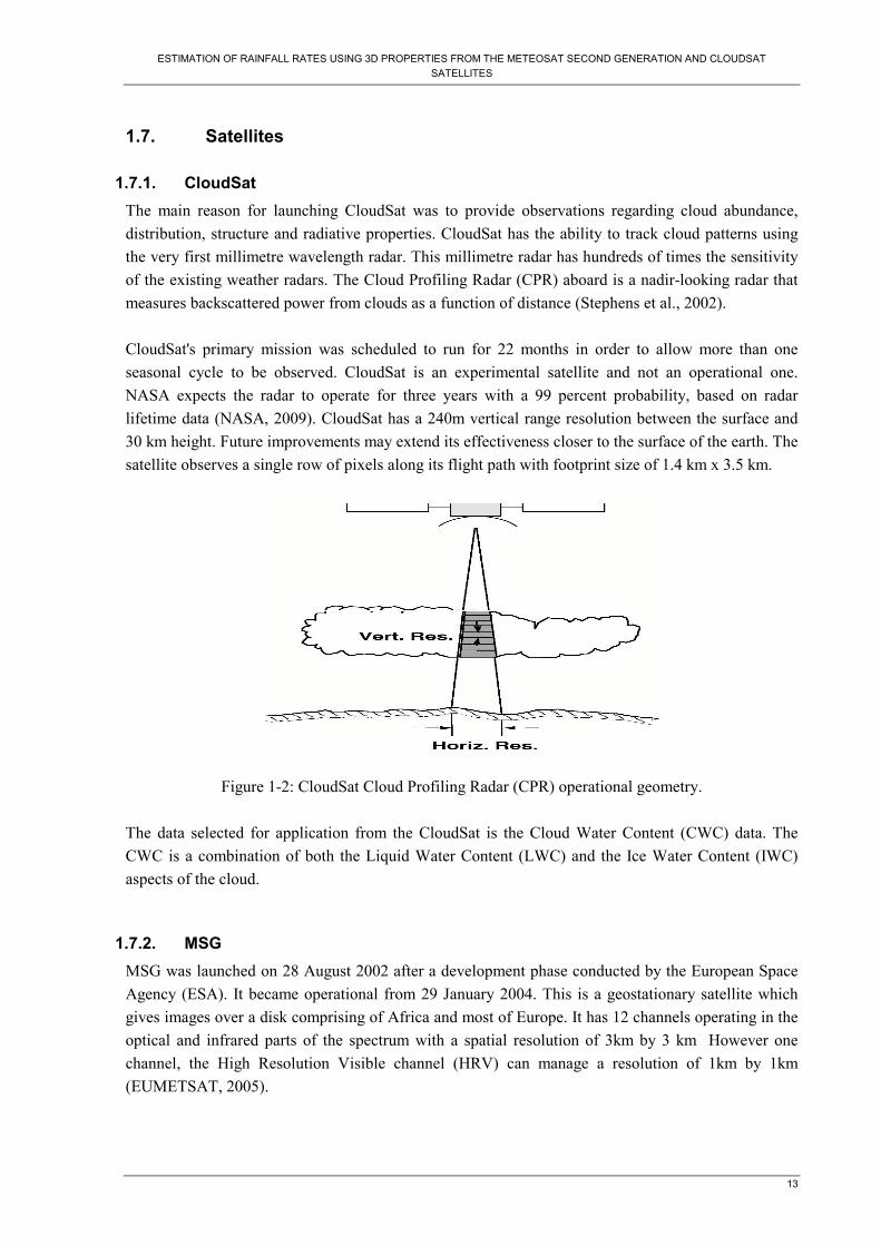
The main reason for launching CloudSat was to provide observations regarding cloud abundance, distribution, structure and radiative properties. CloudSat has the ability to track cloud patterns using the very first millimetre wavelength radar. This millimetre radar has hundreds of times the sensitivity of the existing weather radars. The Cloud Profiling Radar (CPR) aboard is a nadir-looking radar that measures backscattered power from clouds as a function of distance (Stephens et al., 2002). CloudSat's primary mission was scheduled to run for 22 months in order to allow more than one seasonal cycle to be observed. CloudSat is an experimental satellite and not an operational one. NASA expects the radar to operate for three years with a 99 percent probability, based on radar lifetime data (NASA, 2009). CloudSat has a 240m vertical range resolution between the surface and 30 km height. Future improvements may extend its effectiveness closer to the surface of the earth. The satellite observes a single row of pixels along its flight path with footprint size of 1.4 km x 3.5 km.
Figure 1-2: CloudSat Cloud Profiling Radar (CPR) operational geometry. The data selected for application from the CloudSat is the Cloud Water Content (CWC) data. The CWC is a combination of both the Liquid Water Content (LWC) and the Ice Water Content (IWC) aspects of the cloud.
1.7.2. MSG
MSG was launched on 28 August 2002 after a development phase conducted by the European Space Agency (ESA). It became operational from 29 January 2004. This is a geostationary satellite which gives images over a disk comprising of Africa and most of Europe. It has 12 channels operating in the optical and infrared parts of the spectrum with a spatial resolution of 3km by 3 km However one channel, the High Resolution Visible channel (HRV) can manage a resolution of 1km by 1km (EUMETSAT, 2005).

ESTIMATION OF RAINFALL RATES USING 3D PROPERTIES FROM THE METEOSAT SECOND GENERATION AND CLOUDSAT SATELLITES
14
The range of wavelengths of the MSG channels varies from the visible range at 0.6µm wavelength to 12 µm Infra Red wavelength. Each of the wavelengths has unique capabilities of detecting the unique characteristics of the clouds, even though some may overlap from one channel to another. The table below summarized the list of MSG Channels and their respective detection capabilities. Table 1: Characteristics of the SEVIRI Imaging Channels Channel Name Central
Wavelength (µm)
Applications
01 VIS 0.6
0.635 Cloud detection and tracking, scene identification, land surface and aerosol monitoring and generation of vegetative indices 02 VIS
0.8 0.81
03 NIR 1.6
1.64 Discrimination between snow and cloud; and ice and water clouds. Provision of aerosol information.
04 IR 3.9 3.90 Night detection of low clouds and fog. Land and sea temperature determination at night and detection of wildfires.
05 WV 6.2
6.25 Measurement of mid-atmospheric water vapour content and provision of tracers for atmospheric winds. Height assignment for transparent clouds. Each channel representing a different layer.
06 WV 7.3
7.35
07 IR 8.7 8.70 Quantitative information on thin cirrus clouds and discrimination between ice and water clouds.
08 IR 9.7 9.66 Responsive to ozone concentration in the lower stratosphere. Used to monitor total ozone and assess diurnal variability. Potential for tracking ozone patterns as an indicator of wind fields at that level.
09 IR 10.8
10.80 Each responds to the temperature of clouds and the surface; used jointly to assist reduce atmospheric effects when measuring surface and cloud-top temperatures. Also used for cloud tracking, for atmospheric winds and for estimation of atmospheric instability.
10 IR 12.0
12.00
11 IR 13.4
13.40 A CO2 absorption channel. Estimation of atmospheric instability and temperatures of the lower troposphere. Supports height assignment of semi-transparent clouds.
12 HRV 0.4 -1.1 Broadband visible channel. Similar application as the VIS 0.6 but with an improved resolution of 1km by 1km.

ESTIMATION OF RAINFALL RATES USING 3D PROPERTIES FROM THE METEOSAT SECOND GENERATION AND CLOUDSAT SATELLITES
15
2. Theory The assumed vertical distribution of a cloud influences the precipitation as predicted by models, for example assumptions about the cloud vertical structure directly influences the seeder-feeder precipitation mechanism in large scale models (Jakob et al., 1999). Also, the identification of cloud property thresholds in terms of temperature and other qualities is useful in the development of such algorithms.
Direct measurements of vertical structures of clouds have until now been confined to ground –based radar sites, which in most places are not adequate. More direct approaches to obtain global-scale scrutiny of vertical cloud structure depend on water vapour variations observed by the radio-sonde network all over the world. Studies have shown that overlapping cloud layers occur, on the average, about 40% of the time. This may vary from 10% in the case of deserts and mountains to about 80% in the tropical convective zones (Poore et al., 1995). Retrieval can be performed using:
• Optical
• Radar, (ground and remote sensing)
In the next paragraphs the retrieval from MSG, CloudSat and ground radar will be explained shortly. The complete algorithm creation can be found in the appendix. First the ground radar will be discussed as it serves as a theoretical basis for the other retrievals.
2.1. The Rainfall from Ground Radar
2.1.1. Reflectivity:
Radar reflectivity data are typically obtained in the form of a volume scan, i.e. a sequence of sweeps for increasing antenna elevation angles. A volume scan is available every 5–15 min and consists of data given in polar coordinates. The volume scan reflectivity data, collected on a polar grid with a resolution of about 1 by 1 km, are converted to radar-rainfall maps (or products), the conversion includes applying a Z–R relationship, usually in polar coordinates, averaging the polar grid to a rectangular grid, and selecting or averaging the information on the vertical extent of the storm. In this approach, which we will term the drop size distribution (DSD) approach, Z–R relations are derived from raindrop size distribution observations, typically made at the surface and representing a sample volume of the order 1 m³. Due to the fact that rainfall rate and radar reflectivity factor can both be derived from observed raindrop size distributions, Z–R relations can be computed directed by statistical methods (for example, regression of natural logarithms of reflectivity versus natural logarithms of rainfall rate in the case of power law Z–R relationships). In this approach, a Z–R relationship is selected based on analysis of raindrop size (Krajewski et al., 2002).

ESTIMATION OF RAINFALL RATES USING 3D PROPERTIES FROM THE METEOSAT SECOND GENERATION AND CLOUDSAT SATELLITES
16
The echo power of calibrated weather radars is converted to units of the radar reflectivity Z, a property of distributed scatterers [dimension mm6/m3]. These echo values have been normalized for range. The reflectivity is usually given in logarithmic units (base 10):
LOGZdBZ 10= Equation 2-1 In the radar HDF5 files the reflectivity data are converted to 8-bit integers (0-254) and 255 is used to
indicate "no data". The scale and offset of the conversion are given in the HDF5 file:
5.31*5.0 −= valuedBZ Equation 2-2 Rainfall Intensity: There is a fixed range-independent relation between the reflectivity value Z and the rainfall intensity R [mmhrˉ¹]. The following semi-empirical relation, so-called Z-R relationship, is used (Holleman, 2007b) :
Equation 2-3
or using the logarithmic reflectivity:
0.23200*0.16 += LOGRdBZ Equation 2-4
Examples: 7 dBZ will result in 0.1 mmhrˉ¹, 23 dBZ yields 1 mmhrˉ¹, and so on.
In the radar HDF5 files the reflectivity data are converted to 8-bit integers (0-254) and 255 is used to indicate "no data". The scale and offset of the conversion are given in the HDF5 file:
5.31*5.0 −= valuedBZ Equation 2-5
Using the Z-R relationship, the logarithm (base 10) of the rainfall intensity can be obtained from:
0.23200*0.16 += LOGRdBZ Equation 2-6
A rainfall intensity of 0.1 mmhrˉ¹ is represented by the value 77, 1 mmhrˉ¹ by 109, and so on. A data value 255 is used to indicate that no measurement is available, i.e., beyond 320 km from the radar site. In the ILWIS conversion the formula, the rainfall intensity (R) (mm h¯¹) is given by
R=10^ (value-109)/32 Equation 2-7
6.1*200 RZ =

ESTIMATION OF RAINFALL RATES USING 3D PROPERTIES FROM THE METEOSAT SECOND GENERATION AND CLOUDSAT SATELLITES
17
where in the script, say for the image of 12:40 UTC on 15 May 2009, it was presented as: rain200905151240=10^((RAD_NL25_PCP_NA_200905151240.mpr-109)/32), which was used to derive the radar rainfall intensities.
Figure 2-1: Sample of resultant map on ILWIS, after using the formula that converts reflectivity to rainfall intensity
2.1.2. The range and power of radar
Since radars cannot send and receive at the same time. The transmitted pulse must therefore be very short (or echoes from close range will be lost), and the listening time must be as long as possible. Increasing the transmitted power is subject to engineering constraints and cost. A longer transmission pulse would give more power and better long-range performance, but would reduce the close-range capability (Met Office, 2007b). The returning echo is very much weaker than the transmitted pulse and depends on several factors, like attenuation, absorption of energy by particles/dust/cloud droplets. The returning echo also becomes increasingly weak with distance; due to the inverse square relationship with range (i.e. doubling the range cuts the return power to one quarter). The beam width of many modern types of radar is approximately 1° and, as the target distance increases, only an increasingly small part of the transmitted beam is reflected back to the radar.
2.1.3. Doppler radar
Doppler techniques can be used to increase the accuracy of the forecasts. Depending on the equipment installed it is possible to obtain direction and speed information on the droplets observed out to a range of 100 km from the radar. This data is then used, amongst others, by the Met Office’s Numerical Weather Prediction team for improving the numerical model that is used to forecast the weather. The way Doppler radar works is that two pulses of electromagnetic radiation are transmitted. The first pulse is sent from the radar and the returning echoes are received. Almost immediately a second pulse

ESTIMATION OF RAINFALL RATES USING 3D PROPERTIES FROM THE METEOSAT SECOND GENERATION AND CLOUDSAT SATELLITES
18
is sent from the radar and again the returning echo is received. The computer then analyses these two returned echoes and the movement of the droplets of water is calculated from the change in frequency. This movement is only very slight but it is enough to calculate the wind speed within the cloud and the direction of the water droplets.
2.1.4. Interpreting radar imagery
The radars do not receive echoes from tiny cloud particles, but only from the precipitation-sized droplets. Drizzle is generally too small to be reliably observed but rain, snow and hail are all observed without difficulty. It is important to interpret the radar imagery in terms of the beam’s elevation and ‘width’ and the earth’s curvature. For example, the latter means that echoes come from an increasingly higher level the further away precipitation is from the radar. Thus at a range of 100 km, the radar beam is being reflected from the raindrops in a cloud at a height of 1.5 km, but beneath that level rain may be falling from the cloud which the radar misses. For this and other reasons (listed below), the radar rainfall display may not fully represent the rainfall observed at the ground.
2.1.5. Causes of Error
Errors in the received signal can also arise from either meteorological or non-meteorological causes as listed below:-
2.1.5.1. Meteorological Causes of Error
• Radar beam above the cloud at long ranges. Even with a beam elevation of only 1°, individual radar may not detect low-level rain clouds at long distances. A network of overlapping radars helps to minimize this problem.
• Evaporation of rainfall at lower levels beneath the beam. Precipitation detected by the radar at high levels may evaporate if it falls through drier air nearer the ground. The radar rainfall display will then give an over-estimate of the actual rainfall.
• Orographic enhancement of rainfall at low levels. The rather light precipitation which is generated in layers of medium-level frontal cloud can increase in intensity by sweeping up other small droplets as it falls through moist, cloudy layers at low levels. This seeder - feeder mechanism is very common over hills, resulting in very high rainfall rates and accumulations. Even with a network of radars, the screening effect of hills can make the detection of this orographic enhancement difficult, resulting in an under-estimate of the actual rainfall.
• Bright Band. Radar echoes from both raindrops and snowflakes are calibrated to give correct intensities on the rainfall display. But at the level where the temperature is near 0°C, melting snowflakes with large, wet, reflective surfaces give strong echoes. These produce a false band of heavier rain, or bright band, on the radar picture.
• Drop sizes of precipitation within a cloud. Every cloud has a different composition of droplets; in particular, frontal rainfall clouds differ from convective shower clouds. In deriving rainfall rates from radar echo intensities, average values for cloud compositions are used. Radars under-estimate the rain from clouds composed of smaller-than-average drops

ESTIMATION OF RAINFALL RATES USING 3D PROPERTIES FROM THE METEOSAT SECOND GENERATION AND CLOUDSAT SATELLITES
19
(e.g. drizzle), and over estimate the rain falling from clouds with very large drops (e.g. showers). However, averaging the rain over 5 km squares on the radar rainfall display reduces the peak intensities in convective cells.
• Anomalous propagation. Radar beams are like light beams, in that they travel in straight lines through a uniform medium but will be bent (refracted) when passing through air of varying density. When a low-level temperature inversion exists, the radar beam is bent downwards and strong echoes are returned from the ground, in a manner akin to the formation of mirages. This usually occurs in anticyclones, where rain is unlikely and so anomalous propagation is normally recognized without difficulty.
2.1.5.2. Non-meteorological Causes of Error
• Permanent echoes (occultation). These are caused by hills or surface obstacles blocking the radar beam, and are often referred to as clutter. Clutter is rarely seen on radar imagery as it can be mapped on a cloudless day, and then taken out or subsequent pictures by the on-site computer. Occultation is caused by the radar beam being obstructed by a hill or building. A network of overlapping radars helps to minimize this problem.
• Spurious echoes. These may be caused by ships, aircraft, sea waves, and chaff in use on military exercises, technical problems or interference from other radars. The patterns formed by spurious echoes are short-lived, and can usually be identified as they look very different from genuine precipitation echoes.
2.1.6. Advantages and Disadvantages of the Weather Radar
The merits and demerits of use of the weather radar for rainfall intensity estimation are listed below:-
• Advantages: o Detailed, instantaneous and integrated rainfall rates o Areal rainfall estimates over a wide area o Information in near-real time o Information in remote land areas and over adjacent seas o Location of frontal and convective (shower) precipitation o Monitoring movement and development of precipitation areas o Short-range forecasts made by extrapolation o Data can be assimilated into numerical weather prediction models
• Disadvantages:
o Display does not show rainfall actually at the surface o Display may also shows non-meteorological echoes o Estimates liable to error due to technical and meteorological related causes

ESTIMATION OF RAINFALL RATES USING 3D PROPERTIES FROM THE METEOSAT SECOND GENERATION AND CLOUDSAT SATELLITES
20
2.2. Detailed CloudSat Algorithms
2.2.1. Ice Water Algorithm This algorithm tries to differentiate between the ice, mixed phases, and water droplets in the clouds putting emphasis on the ice and the mixed phase droplets.
2.2.2. Forward model and measurements The retrieval combines both active and passive remote sensed data whenever both are available. The vertical profiles of the backscatter are provided by the radar measurements while the vertical integral of a moment of the cloud particle distribution are provided by optical measurements from passive data.
2.2.3. The physics behind
The forward model, derived by (Benedetti et al., 2003) assumes a modified gamma size distribution of the ice crystals (Austin, 2003; Austin, 2004).
−
−Γ
=−
nnnT D
DDD
DNDn exp
1)(
1)(
1ν
γ ν Equation 2-8
where: NT is the ice particle number concentration,
D is the (equivalent) diameter; Dn is the characteristic diameter, υ is the width parameter.
The ice water content (IWC) and the effective radius re are defined in terms of moments of the size
distribution
dDDDnIWC i3)(
6 γπρ=
Equation 2-9
The ice water content (IWC) and the effective radius re are defined in terms of moments of the size distribution
∫
∫∞
∞
=
0
2
0
3
)(
)(
21
dDDDn
dDDDnre
γ
γ Equation 2-10
Where ρi is the density of ice In the case of thin cloud ice particles, these particles are sufficiently small to be modeled as Rayleigh scatterers at the CloudSat radar wavelength and yet sufficiently large that their extinction efficiency approaches 2 for visible wavelengths. These assumptions yield the following definitions of radar reflectivity factor Z and visible coefficient σ ext:
dDDDnZ ray6
0)(∫
∞= γ Equation 2-11

ESTIMATION OF RAINFALL RATES USING 3D PROPERTIES FROM THE METEOSAT SECOND GENERATION AND CLOUDSAT SATELLITES
21
dDDDnext2
0 4)(2πσ γ∫
∞=
Equation 2-12
By applying Equation 2-8 for the size distribution in Equation 2-9 through Equation 2-12 this yields the following equations for the various cloud properties.
)()()(
)3(6
3 zDzNIWC nTi ννπρΓ+Γ
= Equation 2-13
ne Dr2
)2( +=ν
Equation 2-14
)()()(
)2(2
2 zDzN nText ννπ
σΓ+Γ
= Equation 2-15
)()()(
)6( 6 zDzNZ nTray ννΓ+Γ
= Equation 2-16
All of the above properties are functions of position within the cloud column, and we can therefore write IWC (z), re(z), σext (z) , and ZRay (z). We can also specify the columnar ice water content or simply the Ice water path (IWP) as
∫=top
base
z
zdzzIWCIWP )( Equation 2-17
The parameters NT(z), Dn(z) and ν(z) fully define the size distribution. In practice, the measured data are limited to a single radar reflectivity, Z, for each radar resolution bin plus one value of visible optical depth τ for the entire vertical profile. It, therefore, becomes unavoidable to make assumptions by reducing our number of unknowns to be retrieved. Examples are that the number concentration NT and the distribution width ν are assumed to be constant with height. In addition, the distribution width is fixed in the forward model to a specified model for a given scenario. This value is selected based on the cloud type and location. Reference values for each of these categories are obtained from a database of values collected from published statistics of in situ measurements.
2.2.4. Liquid water algorithm The liquid cloud retrieval algorithm is a modification of the method described by Austin and Stephens 2001. The forward model developed for the retrieval assumes a lognormal size distribution of cloud droplets (Austin, 2003)):
−=
2log
2
log 2
lnexp
2)(
σσπgTrr
r
NrN
Equation 2-18

ESTIMATION OF RAINFALL RATES USING 3D PROPERTIES FROM THE METEOSAT SECOND GENERATION AND CLOUDSAT SATELLITES
22
where NT is the droplet number density, r is the droplet radius, and, rg, σlog, and σg are defined by
rrg lnln = Equation 2-19
gσσ lnlog = Equation 2-20
( )22 lnln gg rr −=σ Equation 2-21
where rg is the geometric radius, σlog is the distribution width parameter, σg is the geometric standard deviation, ln is the natural (base e) logarithm.
The liquid water content (LWC) and the effective radius re are defined in terms of moments of size
distribution.
drrrNLWC 3
0 34
)( πρω∫∞
=
Equation 2-22
∫
∫∞
∞
=
0
2
0
3
)(
)(
drrrN
drrrNre Equation 2-23
where ρω is the density of water, For clouds with negligible drizzle and precipitation, cloud droplets are sufficiently small to be modelled as Rayleigh scatterers at the CloudSat radar wavelength and sufficiently large that their extinction efficiency approaches 2 for visible wavelengths. The assumptions result to the following equations for radar reflectivity factor Z and visible extinction coefficient σ ext:
drrrNZ ∫∞
=0
6)(64 Equation 2-24
drrrNext ∫∞
=0
2)(2 πσ Equation 2-25
Using Equation 2-18 for the size distribution in Equation 2-22 through Equation 2-25 results in the
following equations for the various cloud properties:
= 2log
3
29
exp3
4 σρπω gT rNLWC Equation 2-26

ESTIMATION OF RAINFALL RATES USING 3D PROPERTIES FROM THE METEOSAT SECOND GENERATION AND CLOUDSAT SATELLITES
23
= 2log2
5exp σge rr Equation 2-27
( )2log
6 18exp64 σgT rNZ = Equation 2-28
( )2log
2 2exp2 σπσ gText rN= Equation 2-29
Similarly, as with the case with IWC, these functions are functions of position in the atmospheric column: we can therefore write, LWC (z), re (z), Z(z) and σext (z) . We can also specify the columnar ice water content or simply the Liquid water path (LWP) as
∫=top
base
z
zdzzLWCLWP )( Equation 2-30
The scattered energy received by the radar from particles at a given range will be attenuated in both directions by cloud particles between that range and the radar receiver. The measured reflectivity factor Z’ will be reduced from the intrinsic reflectivity factor Z according to the following expression:
( ) ( ) ( )
−= ∫
pathabs dzzzZzZ ''' 2exp σ , Equation 2-31
where the path integral is over the portion of the cloud between z and the radar.
2.2.5. Departures from lognormal distribution
The retrieval assumes a lognormal distribution of cloud droplets. Any departures from this distribution will have a degrading effect on the retrieval. One source of such departures is the presence of drizzle or rain within the cloud. Detection criteria for the presence of drizzle or rain are still under development. Since the current procedure only identifies drizzle or precipitation for any case where dBZZ 15'=≥ . At the moment, drizzle/precipitation is identified in the output by setting a flag in the status variable. The algorithm is still run as normal producing output values (unless it diverges). In the case of divergence, the flag serves as an indicator that the solution is most probably unreliable due to non – compliance to the lognormal distribution assumption. It has been found, in practice, that significant presence of precipitation caused a failure of convergence. This resulted in the issuance of error signal (-44.44). The retrieval of cloud properties in the presence of precipitation is a difficult problem due to the sensitivity of the radar to the precipitation-sized particles. The CloudSat research team is trying to solve this problem, and this research is also aimed at getting a solution using cloud ice particle properties as a proxy.

ESTIMATION OF RAINFALL RATES USING 3D PROPERTIES FROM THE METEOSAT SECOND GENERATION AND CLOUDSAT SATELLITES
24
2.3. Retrieval by Optical Remote Sensing Sensors
One of the methods of determining precipitating clouds in use is the comparison of the brightness temperatures of the IR 10.8 µm and WV 6.2 µm MSG images. If the difference is less than 11K, then the cloud is qualified to be a precipitating cloud (pcloud). Then creation of a cloud mask (clm) within ILWIS and later integration of the cloud mask with the precipitating cloud, i.e. one detected by TRMM satellite. The two images are blended from and a correlation between the TRMM or the SSM/I in this case and cloud top temperature from MSG. The general trend follows that rainfall intensity increases with coldness of the cloud top temperature.
2.3.1. Overview
The main inputs to the MPE algorithm are as follows (deriving from two separate satellite sources): • Level 1.5 data from the MSG IR10.8 channel. • Microwave imager data from the SSM/I instruments on board the polar-orbiting satellites of
the US Defence Meteorological Satellite Program (DMSP).
The MSG IR10.8 image data are availed in the form of equivalent black body brightness temperatures (EBBT) in Kelvin (K). The MPE algorithm processes MSG data from channel IR10.8 in near real-time (or some time later in the event of delayed processing) and derives instantaneous rain rates at full MSG pixel resolution. As additional input, external satellite data from the SSM/I instrument are be required from up to 24 hours before the acquisition time of the MSG image (EUMETSAT, 2008).
2.3.2. Algorithm Description
The algorithm consists of two independent steps: the co-location of SSM/I and MSG data, and the product generation on the basis of the co-located data sets. In the framework of Meteorological Products Extraction Facility (MPEF) these two steps are realised by two activities of the MPE software unit, which include the acquisition and the decoding of the SSM/I data files as well as the calculation of rain rates from the SSM/I data at the original SSM/I resolution. The time difference between the measurement of the SSM/I data and the MSG pixel shall be smaller than 10 minutes. The real pixel sensing time and not the image time stamp of the MSG image is relevant in this context. Each co-located data point (CDP) consists of the geographical location of the centre of the SSM/I pixel (latitude and longitude), the rain rate derived from SSM/I data and the co-located average MSG EBBT. The CDPs are stored in intermediate data files. For the product generation the MSG image is divided into processing boxes (PBs) which are equally spaced in latitude and longitude.
2.3.3. Estimation of instantaneous rain rates
The image for channel IR10.8 is read for the reference time of the product generation activity. This step can be done either in real-time or delayed. For a given pixel, the rain-rate estimation is performed only if the scene type is cloudy; otherwise, the rain rate is set to zero. For each pixel of the image the geographical location is calculated. Then the corresponding PB and its surrounding eight PBs are identified. At the edge of the processing area the number of surrounding PBs can be smaller. The look

ESTIMATION OF RAINFALL RATES USING 3D PROPERTIES FROM THE METEOSAT SECOND GENERATION AND CLOUDSAT SATELLITES
25
up tables LUTs of the (up to nine) PBs are used to determine rain rates for the pixel EBBTs. The final rain rate is determined as a weighted mean of the (up to nine) pixel rain rates. For each processing box, there are two Quality Indicators (QIs): a standard deviation and a correlation coefficient. MSG rain rates are first derived from the EBBTs using the LUTs for each CDP. These values are then compared to the initial SSM/I rain rates, by calculating their standard deviation and correlation coefficient. The correlation coefficient can be used to identify areas where the confidence in the rain retrieval is not sufficient. The standard deviation is useful for estimating the accuracy of the SSM/I rain rates themselves.
3. Materials and Methods The main challenge was the creation of an algorithm from CloudSat to eventually be used to improve the MSG rain rate algorithm. It should be noted that the properties of CloudSat are predominantly

ESTIMATION OF RAINFALL RATES USING 3D PROPERTIES FROM THE METEOSAT SECOND GENERATION AND CLOUDSAT SATELLITES
26
vertically oriented while those of MSG SEVIRI are horizontally oriented. Recalling, CloudSat is a polar orbiting satellite with a maximum temporal resolution of about16 days at the equator and about 14 days at the mid latitudes. The other difference between these satellites is in their spatial resolution. MSG boasts of 3km by 3km pixel resolution while CloudSat has 1.4 Km x 3.5 Km oblong Field of View (FoV) with no swath capabilities. It is evident that the two sensors are not perfect in every aspect and they can together be used to complement each other to derive a better method of estimating rainfall rates. This procedure will first involve the download of MSG Precipitation Estimates (MPE) images which contained data on the rainfall rates every 15 minutes derived from both IR and water vapour channels. The next step was to track the flight path of the CloudSat image over Europe which can be found on the NASA website1 as well as the CloudSat website. Data regarding CloudSat path1 and internal cloud properties2 was collected online for various dates within the six months period of summer from March to August 2009 and also for the summer season (May to August) of 2007. This data captured instances of both rainy and non-rainy cloud episodes over Western Europe. The critical selection of the cloud episodes was the collocation of the clouds with an overpass of the CloudSat satellite. Data for the CloudSat Combined Water Content (CWC) hdf images containing information about the merged water and ice content within the vertical extent of the clouds was also downloaded. These hdf files can be downloaded using the Hierarchical Data Format, HDF View software to view their characteristics and attributes (geographic or otherwise) among other details. The next step was to gathering the values of the various cloud properties of CloudSat after importing them from the HDF View. From the HDF View, the cloud vertical profile was downloaded as depicted in Figure 3-1 for the purpose of determining its properties which were later compared with the MPE product to estimate a relationship between the rainfall estimates from SEVIRI and CWC from CloudSat.
• The physical properties of the cloud downloaded from the CloudSat data will be extracted to see which of them and how they contribute to the amount of rainfall emanating from the cloud.
• The cloud physical properties were observed on a profile by profile basis, but considering the high number of profiles on a cloud, and also the fact that CloudSat’s spatial resolution of 1.1 km is higher than that of MSG’s 3km. In order to ensure that the CloudSat readings are not done more than once within the same MSG pixel, I decided to skip every two profiles in the series. An example is considering profiles 1, 4, 7, 10, 13, 16, etc.
1 : http://www-angler.larc.nasa.gov/public/predicts/gif/world/cloudsat/ 2 : http://www.cloudsat.cira.colostate.edu/

ESTIMATION OF RAINFALL RATES USING 3D PROPERTIES FROM THE METEOSAT SECOND GENERATION AND CLOUDSAT SATELLITES
27
• For the purpose of this study, the rain radar data and the daily rain gauge data, where applicable, was assumed to represent the ground truth for the purpose of calibrating the findings from MSG and CloudSat.
• Data from sub Sahara Africa (Kenya) was used to gauge whether the same results could be
used in the tropical cloud scenario.
Figure 3-1: Computer screen snapshot of the data retrieval using the HDF View
3.1. Cloud Types The cloud types were grouped into three main categories, i.e.
• rainy clouds, • Light non- rainy clouds • Dense and drizzle clouds
The profiled data regarding each of the clouds was gathered in order to study the relationship between the observed characteristics and the resultant rainfall.
3.2. MSG Data
The MSG data was collocated for selected dates from the MSG database at the ITC together with the corresponding MPE rain rates for are extracted using the ILWIS software via the pixel information toolbar. Analysis of the various parameters and how they contribute to the rain rates and also how they are related to one another was observed. Figure 3-2 shows a screen shot from the MPE product dated 31 May 2007 at 1300UTC. Red colour indicates regions of highest rainfall intensity while blue are for regions experiencing a dry spell.

ESTIMATION OF RAINFALL RATES USING 3D PROPERTIES FROM THE METEOSAT SECOND GENERATION AND CLOUDSAT SATELLITES
28
Figure 3-2: A screen-shot of MPE product of MSG indication areas of varying rainfall intensities.
3.3. Cloudsat Data
In this study, the Western Europe continent was preferred due to the availability of data, especially radar data to confirm the results from the CloudSat observations vis-à-vis the MPE product. The data on CloudSat CWC for the periods May to August 2007, and March to August 2009 were obtained for the study to correspond with the available radar data for the same dates. The first data to be downloaded by the HDF View is the geo-location in latitude and longitude, stating from first profile labelled as profile no.0 to the last profile either no. 37080 or 37081 in the granule. The corresponding data on cloud property values follow suit with keeping in mind the matching profiles. The cloud property data extracted for this study are listed as follows:
• Number of cloudy bins • Ice Effective radius • Liquid effective radius • Liquid water path • Ice water path • Liquid water content • Ice water content
Other data is not directly available in from the HDF view but can be derived manually such as, number of icy bins2, cloud base height, etc. In this study, one of the challenges was that the CloudSat temporal resolution and areal coverage are low. Since the satellite rotates around the earth about 14 times a day and its return period is 14-16
2 Note that: Data for the number of icy bins is convenient when calculating the profile’s mean ice characteristics such as effective radius and ice water path. The direct use of no. of cloudy bins in such calculations may cause errors since not all cloudy bins may be icy at any particular moment.

ESTIMATION OF RAINFALL RATES USING 3D PROPERTIES FROM THE METEOSAT SECOND GENERATION AND CLOUDSAT SATELLITES
29
days depending on the latitude, only cases of CloudSat overpasses that coincided with various clouds categorized in terms of possibilities of them precipitating were used. As had been described earlier in this study, due to the nature of liquid water droplets diverging, especially immediately before and during precipitation, ice water quantities which are more robust under similar conditions were used as proxy data.
Figure 3-3: Image of the vertical cross-section of a CloudRadar Data (NASA) Figure 3-3 depicts an image of clouds along the CloudSat path over Northern France on 9 May 2007 between 02:15:05 and 02:18:16. The thick cloud is clearly visible at the centre of the image while the date and time of flight and the geographical location are also indicated.
3.4. Retrieval by Ground Radar Sensors
Weather radars use electromagnetic radio waves to measure precipitation and other airborne matter in the atmosphere (Rinehart, 2004). The radar releases pulses into the atmospheric targets, which bounce back as echoes.
Difficulties in the retrieval of precipitation through remote sensing radar sensors are enhanced because of the sensitivity of radar sensors. One fact is that clouds are weak scatterers of microwave radiation. The radar is supposed to achieve the maximum possible sensitivity and hence maximize cloud detection. This sensitivity is basically determined by radar-received power. Unfortunately some degree of noise level accompanies this signal. Optimization of this sensitivity involves a careful compromise between six competing and sometimes conflicting factors: cloud backscattering properties, the vertical resolution, available electrical power delivered to the radar system, satellite orbit altitude, the radar technology, and atmospheric attenuation. Even though the received signal can be enhanced by increasing the antenna size and transmitter output power; an antenna diameter is limited by launch limitations while the power is also restricted by transmitter technology and power supply capability of the spacecraft. The amount of radiation received is also determined by the cloud reflectivity and the prevailing atmospheric attenuation. The cloud reflectivity increases with increasing radar frequency, however, the atmospheric attenuation becomes prohibitive at higher frequencies.

ESTIMATION OF RAINFALL RATES USING 3D PROPERTIES FROM THE METEOSAT SECOND GENERATION AND CLOUDSAT SATELLITES
30
After considering all the above-mentioned factors, 94 GHz (3.19 mm wavelength) was found to be the optimum the operating frequency as showed an increase of 33dB over the 14 GHz (2.14 cm wavelength) TRMM radar (Stephens et al., 2002). The intensity of the echoes or radar reflectivity is converted to a radar reflectivity factor Z by use of the Rayleigh scattering approximation (Probert-Jones, 1962).
∑=i
iDZ 6 Equation 3-1
where D= diameter of raindrops for
i= number of raindrops per unit volume
The formula seems to work well when the radar wavelengths (3-10 cm) are larger than raindrop diameters (<6 mm). A simpler exponential form of the drop size distribution was suggested by (Marshall et al., 1948) in the form
)exp()( 0 DNDN Λ−= Equation 3-2
Where the drop density N0=8 x 103mm-1m-3,
Λ= (4.1R-0.21mm-1), and R is the rain rate in mmh-1.
The radar reflectivity factor can be approximated from the sixth moment of the drop size distribution:
( ) 47.170
6 290/720 RNdDDDNZ =Λ== ∫ Equation 3-3
Actually, many Z-R relationships have been derived depending on the actual meteorological conditions (e.g. cloud types). One of the most popular of these is given as:-
6.1200RZ = Equation 3-4
The first step should involve the converting of vertical profiles of Z into meaningful microphysical data quantities. An algorithm is therefore being developed for identifying cloud types and precipitation. Another more recent method is the application of the Vertical Profile of Reflectivity (VPR). However, measurements derived from the profiler have fallen short of expected accuracy due to the presence of significant gradient resulting in gross underestimation of the QPE.
3.4.1. Ground radar
The radar data was obtained courtesy of the Royal Netherlands Meteorological Institute (KNMI) and can be divided into two sets. The first set covers the Netherlands and comprised of two KNMI radars. One located is in De Bilt, in the centre of the Netherlands (52.10°N, 5.18°E) while the other is at Den Helder, in Northern part of the Netherlands (52.96°N, 4.79°E).. Both radars have a range of

ESTIMATION OF RAINFALL RATES USING 3D PROPERTIES FROM THE METEOSAT SECOND GENERATION AND CLOUDSAT SATELLITES
31
approximately 165 Km (Holleman, 2007a). These radar images overlap to cover Netherlands, most of Belgium, Western Germany, and the part of the North Sea. The second set of data comprised of overlapping network of radars covering Western Europe from the Operational Programme on the Exchange of Weather Radar Information (OPERA) project under the Network of European Meteorological Services (EUMETNET), see Figure 3-4. The data was in HDF5 format showing the backscatter reflectivity in 8 bit, i.e. values ranging from 0 – 255. For proper viewing in ILWIS, the image underwent transformation in terms of projection as shown in appendix part 1. The re-projection was done in ILWIS using tie points based on location of the European radar network bases. The rainfall values for both MSG and radar were derived from ILWIS on pixel by pixel analysis corresponding to the CloudSat flight of path. Figure 3-4 shows the backscatter reflectance radar image of clouds over most of Western Europe from the OPERA Network in 8 –bit (0-254). Values of 255 represent areas beyond the radar network. This data is later fine-tuned using the formula for conversion to rainfall rates to give the images as shown in panel on the right hand side.
Figure 3-4: Data from the Opera Network. In the left panel, the backscatter radar image is shown, for 31 May 2007, 13:00 UTC from the OPERA radar Network, (source KNMI). In the right panel, the retrieved rain rates are shown for 31 May 2007, 13:00 UTC.
Figure 3-5 shows the generalised flow chart of step by step activities of carried this in this research beginning with the data acquisition from the different sources, its analysis and finally the creation of the simple algorithm.
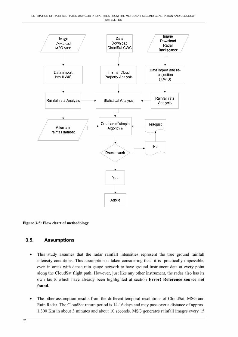
ESTIMATION OF RAINFALL RATES USING 3D PROPERTIES FROM THE METEOSAT SECOND GENERATION AND CLOUDSAT SATELLITES
32
Figure 3-5: Flow chart of methodology
3.5. Assumptions
• This study assumes that the radar rainfall intensities represent the true ground rainfall
intensity conditions. This assumption is taken considering that it is practically impossible, even in areas with dense rain gauge network to have ground instrument data at every point along the CloudSat flight path. However, just like any other instrument, the radar also has its own faults which have already been highlighted at section Error! Reference source not found..
• The other assumption results from the different temporal resolutions of CloudSat, MSG and
Rain Radar. The CloudSat return period is 14-16 days and may pass over a distance of approx. 1,300 Km in about 3 minutes and about 10 seconds. MSG generates rainfall images every 15

ESTIMATION OF RAINFALL RATES USING 3D PROPERTIES FROM THE METEOSAT SECOND GENERATION AND CLOUDSAT SATELLITES
33
minutes (say 11:00, 11:15,11:30 and 11:45 UTC) while the rain radar produces products every five minutes (e.g. 11:00, 11:05, 11:10, 11:15 UTC, …etc). To minimize the disparities, the time for the CloudSat overpass was considered first. The MSG time was considered next depending on weather the overpass was close to the end of the 15 minute interval or at the beginning. If closer to the beginning, it is allocated the previous 15 minute slot while if closer to the end, it is given the end of the current 15 minute slot. The radar data was then considered last depending on which 5 min image was closest to the CloudSat time of overpass.
• There exists a problem of parallax with cloud images or regions outside the tropics. Cloud
may appear to cover an area from the MSG image and yet in reality they may be off by several Kilometres. This problem may be inherent especially when comparing data, pixel by pixel which is likely to introduce errors.
• Whenever CloudSat encounters a cloud which is precipitating or about to, the data on the liquid water properties of the cloud diverges and is impossible to draw quantitative conclusions from it. It was decided that ice data be used as a proxy across the board for uniformity even to non-rainy clouds.

ESTIMATION OF RAINFALL RATES USING 3D PROPERTIES FROM THE METEOSAT SECOND GENERATION AND CLOUDSAT SATELLITES
34
4. Results Fourteen different clouds all over the study area were investigated and then later categorized into three major groups, of cloud scenarios. The three cloud scenarios created were the rainy clouds, the non- rainy clouds and the dense with or without drizzle which CloudSat encountered along its flight path.
4.1. Dense and Drizzle Clouds
4.1.1. Case 1: Dense cloud in Belgium
In this case the correlation coefficient between the mean ice effective radius and the MSG rainfall rates was 0.85, and that for Ice water path and the MSG rainfall rates was 0.91. In the actual sense however, the radar information available indicates that no actual precipitation occurred though the cloud appeared ‘dark’. Observing the cloud’s bins at every fourth profile, gave the results as shown in the table above. Other relationships between the cloud properties showed consistent results as given in the graphs below. Table 4-1: Summary of the different internal cloud properties of a dense, non–precipitating cloud by CloudSat over Belgium on 4 May 2009.
No of cloudy bins
No. of icy bins
Ice water path (gmˉ³)
Liquid water path (Kgmˉ²)
Mean ice eff. Radius (µm)
Mean ice water content (mgmˉ³)
MSG rainfall rate (mmhˉ¹)
Radar rainfall rate (mmhˉ¹)
Max 33 33 13.8 2.36 6.07 2.08 2.76 0.00 Min 13 13 1.8 0.07 4.99 0.43 0.00 0.00 Mean 22.83 22.81 6.72 0.89 5.58 1.18 0.82 0.00 Std Dev 6.63 6.62 3.61 0.68 0.33 0.46 0.87 0.00
The scenario depicts a moderately thick cloud either approaching maturity and almost precipitating or decaying and probably just after precipitating. This is shown by the relatively high number of cloudy and icy bins in the vertical profile. Table 4-1shows that the observed cloud has relatively low ice water content in it. This could be a factor in hindering its ability to producing rainfall. The cloud may have not have gathered enough “mass” to make it heavy enough to overcome air resistance be pulled by gravity from high up in the atmosphere to the ground. The MSG algorithm may have picked a wrong signal due to the long profile of the cloud, making it have a low cloud-top temperature. However, the cloud internal properties show that the cloud is not mature enough; it has a low cloud water path and ice water content. The mean ice effective radius could be high, but only located at the top-most part of the cloud.

ESTIMATION OF RAINFALL RATES USING 3D PROPERTIES FROM THE METEOSAT SECOND GENERATION AND CLOUDSAT SATELLITES
35
Figure 4-1: Graph above showing the variation between ice water path and ice effective radius. Figure 4-1 shows how some of the cloud properties are closely correlated to one another. Increase in ice water path within the cloud results into a higher mean ice effective radius.
Figure 4-2: Variation of the mean Ice effective radius per bin with the number of cloudy bins in the profile Figure 4-2 above depicts the relationship between the Mean ice effective radius and the no. of cloudy bins within the profile. It shows an increase of cloudy bins being indicative of bigger mean ice effective radius, though the change is very gradual. In this case the MSG rain rate algorithm gave a ‘false’ rainfall alarm. This may have been contributed by the MSG algorithm that mainly relies on the cloud-top temperature difference values. This is especially for the higher latitudes, which are out of the operational range of the TRMM that provides complementary radar data. This cloud must have been deficient of important constituents which could have enabled it to produce precipitation.

ESTIMATION OF RAINFALL RATES USING 3D PROPERTIES FROM THE METEOSAT SECOND GENERATION AND CLOUDSAT SATELLITES
36
4.1.2. Case 2: Drizzle cloud in S. West Netherlands Table 4-2: Light rain cloud, South West Netherlands, 13 May 2009, 1250 UTC
No of cloudy bins
No. of icy bins
Ice water path (gmˉ³)
Liquid water path (Kgmˉ²)
Mean ice effective Radius (µm)
Mean ice water content (mg mˉ³)
MSG rainfall rate (mmhˉ¹)
Radar rainfall rate (mmhˉ¹)
Max 22 15 35.2 7.30 9.38 10.45 0.00 0.60 Min 0 0 0.00 0.00 0.00 0.00 0.00 0.00 Mean 22.83 22.81 6.72 0.89 4.71 1.20 0.00 0.07 Std Dev 6.63 6.62 3.61 0.68 0.33 2.28 0.00 0.12
The above table highlights the of the cloud internal properties for the cloud over the South Western part of the Netherlands. It can be noted that the MSG rainfall rates algorithm did not qualify this cloud as capable of giving precipitation. On the other hand, the Doppler rainfall radar managed to detect rainfall intensities although; the individual the pixel with the highest amount generated only 0.6 mmhˉ¹. The cloud properties in this case appear to lie in the thin line that determines whether the cloud is mature enough to produce rain or not. None of the cloud properties is either too high or too low, and such clouds may be critical in providing algorithms for rainfall determination in clouds.
4.1.3. Case 3: Drizzle cloud: N.E Netherlands and E. Germany This cloud showed an extreme case of very light rain. The cloud has generally low values for ice water path and ice water content and fairly high value of ice effective radius. This is a case of a drizzle cloud emanating from a relatively thin cloud. Table 4-3: Summary of internal cloud properties from CloudSat on a cloud over N.E Netherlands and W. Germany on 15 May 2009 at about 12:40 UTC. No of
cloudy bins
No. of icy bins
Ice water path (g mˉ²)
Liquid water path* (Kg mˉ²)
Mean ice eff. Radius (µm)
Mean ice water content (mg mˉ³)
MSG rainfall rate (mmhˉ¹)
Radar rainfall rate (mmhˉ¹)
Max 25 17 8.20 7.18 9.46 3.42 0.00 0.04 Min 0 0 0.00 0.00 0.00 0.00 0.00 0.00 Mean 6.79 4.23 0.72 1.05 4.26 0.34 0.00 0.00 Std dev 6.64 4.31 1.36 1.97 2.65 0.55 0.00 0.00
Looking into the values of the LWP derived from the cloud it can be observed that some of the profiles do not follow the log-normal distribution. This is an indication of some significant instability in the cloud, reiterating its potential to produce some rainfall. The cloud’s IWP and IWC are comparatively small even though they seem to have an ice efficient radius with a mean of 4.26µm and

ESTIMATION OF RAINFALL RATES USING 3D PROPERTIES FROM THE METEOSAT SECOND GENERATION AND CLOUDSAT SATELLITES
37
a max of 9.46µm. This could be indicative of a shallow layer of ice droplets in the cloud, barely enough to warrant substantial rainfall.
Figure 4-3: Graph showing the relationship between the mean RE and the mean IWC in a cloud during CloudSat overpass in N.E Netherland and W. Germany on 15 May 2009 at 12:40 UTC.
4.1.4. Case 4: Drizzle cloud over W. Germany, 10 June 2009 The Table 4-4 shows a case of a thin low cloud which gave yield to some light rain or drizzle. The flight path of the satellite must have encountered areas of no cloud coverage but the data shows that the cloud had a shallow vertical extent with low IWP and IWC but relatively high RE. Table 4-4: Summary table of internal cloud properties of a drizzle cloud over West of Germany on 10 June 2009 at about 02:05 UTC No of
cloudy bins
No. of icy bins
Ice water path (g mˉ²)
Liquid water path* (Kg mˉ²)
Mean ice eff. Radius (µm)
Mean ice water content (mg mˉ³)
MSG rainfall rate (mmhˉ¹)
Radar rainfall rate (mmhˉ¹)
Max 12 5 2.10 7.17 10.02 1.76 0.00 0.17 Min 0 0 0.00 0.00 0.00 0.00 0.00 0.00 Mean 4.62 2.24 0.20 1.76 4.38 0.20 0.00 0.01 Std dev 4.32 2.06 0.47 2.32 3.68 0.40 0.00 0.03
4.2. Precipitating Clouds
4.2.1. Case 1: United Kingdom, 27 May 2007 This was the case of a cloud in the United Kingdom that was observed on 27 May 2007 in which it experienced rainfall. Both the MSG and radar rainfall estimation was done together with the analysis of the cloud properties from CloudSat, see Table 4-5.

ESTIMATION OF RAINFALL RATES USING 3D PROPERTIES FROM THE METEOSAT SECOND GENERATION AND CLOUDSAT SATELLITES
38
Table 4-5: Summary of cloud properties from CloudSat during a rainy episode over the United Kingdom on 27 May 2007 No of
cloudy bins
No. of icy bins
Ice water path (g mˉ²)
Liquid water path* (Kg mˉ²)
Mean ice eff. Radius (µm)
Mean ice water content (mg mˉ³)
MSG rainfall rate (mmhˉ¹)
Radar rainfall rate (mmhˉ¹)
Max 34 30 213.70 3.02 10.59 32.11 4.16 5.23 Min 0 0 0.00 0.00 0.00 0.00 0.00 0.00 Mean 21.68 1.21 44.59 1.21 7.77 7.70 1.16 0.69 Std dev 8.34 1.06 41.31 1.06 1.64 6.00 1.26 0.88
Variations within the cloud of the different inherent properties can be noticed in Table 4-5. The value for the liquid ware path is low due to the fact that most of its layers indicate errors after the diverged from the lognormal distribution assumed by the algorithm used by CloudSat. From the data that derived Table 4-5, most of the profiles had the LWP data diverged from the log-normal distribution. The figure for maximum LWP of 3.02 Kgmˉ² shown above applies only to the retrievable LWP data. This is indicative of a highly unstable cloud with a high probability of producing rainfall. One other observation is that the CloudSat overpass encountered ‘empty’ spaces within this cloud series resulting in zero value as minimum for all cloud properties. Since properties associated with ice are more robust (don’t easily diverge) compared to those of liquid nature, it can be noticed that this cloud had a mean of 44.59 gm¯² with a peak of an impressive 213.7 gm¯² was producing some precipitation during this time.
Figure 4-4: Graph showing the direct relationship between the IWP and the Number of Cloudy bins The Figure 4-4 shows that it may takes about 10 cloudy bins to create noticeable ice droplets which are essential for the condensation process that leads to precipitation. Also, it can be noticed that having more than 10 cloudy bins is no guarantee for increase in the ice water path. This is an indicator

ESTIMATION OF RAINFALL RATES USING 3D PROPERTIES FROM THE METEOSAT SECOND GENERATION AND CLOUDSAT SATELLITES
39
that there are other factors, other than the no of cloudy bins that might contribute to a cloud column with bigger ice water path.
In this study, differentiation between the number of cloudy bins (bins with either ice or water droplets or both) and that of icy bins (those that at exclusively consist of ice particles) was done. The reason was that not all cloudy bins have ice particles in them. The icy bins were therefore derived through manual counting, were used in the computation of the mean ice effective radius per cloud profile.
Figure 4-5: Graph showing the variation between the mean ice water content and the resultant rainfall intensity. Figure 4-5 shows the relationship between the mean IWC of a profile in relation to the resultant rainfall per pixel from the weather radar. The general idea is that the IWC is rarely zero within the cloud but at some threshold, it enables the cloud to produce rainfall.
Figure 4-6:Graph showing the variation between the MSG rainfall rates and those of the Radar Radar The graph on Figure 4-6 depicts that the MSG generally overestimated the rainfall for the UK on 27 May 2007. Expect for few ocassions where the radar detected a few narrow ‘spikes’ of higher rainfall,

ESTIMATION OF RAINFALL RATES USING 3D PROPERTIES FROM THE METEOSAT SECOND GENERATION AND CLOUDSAT SATELLITES
40
the MPE product recorded higher rainfall than that of the radar. This can be attributed to the higher spatial resolution of the weather radar than that of the MSG.
Figure 4-7: Graph depicting direct relationship between mean ice effective radius within a profile with the corresponding number of icy bins. In clouds studied, it had become evident as shown in Figure 4-7 that the ice effective radius increases with the number of icy bins in the cloud vertical column. This indicates that as a cloud grows, so the chances that it develops larger ice droplet radius too, and therefore increases the chances of the occurrence of rainfall.
4.2.2. Case 2: Southern France, 31 May 2007
This was a case of a thick mature and precipitating cloud over S. France that was profiled by CloudSat on 31 May 2007 at around 12:50 UTC. The cloud gives high average and maximum values for both the no. of cloudy and icy bins, ice water path, ice effective radius and IWC. It can be noticed that both the MSG and radar rainfall give fairly high amounts of precipitation. Also to be noted is that CloudSat encounters regions free of cloud cover along its path, which is the reason why the minima may be reading zero for some most parameters. Table 4-6: Summary of the internal cloud properties from CloudSat over Southern France, 31 May 2007.
No of cloudy bins
No. of icy bins
Ice water path (gmˉ³)
Liquid water path* (Kgmˉ²)
Mean ice eff. Radius (µm)
Mean ice water content (mg mˉ³)
MSG rainfall rate (mmhˉ¹)
Radar rainfall rate (mmhˉ¹)
Max 40 33 217.60 6.50 10.59 32.38 4.64 10.75 Min 0 0 0.00 0.00 0.00 0.00 0.00 0.03 Mean 28.98 23.94 47.95 1.45 7.77 7.79 1.81 1.09 Std dev 8.34 1.06 42.11 2.06 1.64 6.30 1.26 2.20
4.2.3. Case 3: Northern France, 9 May 2007
This was another case of a rainy cloud observed in Northern France on 9 May 2007 as illustrated in Table 4-7. The rainfall may not have been heavy and unfortunately the radar image for this time is

ESTIMATION OF RAINFALL RATES USING 3D PROPERTIES FROM THE METEOSAT SECOND GENERATION AND CLOUDSAT SATELLITES
41
missing. It can, however, be observed that like the previous clouds over UK and S. France, this one has the properties of a rainy cloud as shown in the table below. Table 4-7: Summary of the internal cloud properties from CloudSat over Northern France, 9 May 2007
No of cloudy bins
No. of icy bins
Ice water path (g mˉ³)
Liquid water path* (Kg mˉ²)
Mean ice eff. Radius (µm)
Mean ice water content (mgmˉ³)
MSG rainfall rate (mmhˉ¹)
Radar rainfall rate (mmhˉ¹)
Max 43 37 157.00 13.26 9.34 19.81 0.80 N/A Min 2 0 0.00 0.00 0.00 0.00 0.00 N/A Mean 25.63 20.73 33.29 3.85 6.77 4.18 0.03 N/A Std dev 12.13 11.22 43.31 3.28 1.50 4.98 0.15 N/A
Fig 4-8 shows how the ice water content varies with the number of bins containing ice particles within a profile. The increase in icy bins is an indication of the development processes within the cloud that are active in condensing water vapour around condensation nuclei. As more layer of the cloud are involved, the more water in attracted and the higher the ice content per cubic volume. From the graph, amounts of 10 mgmˉ³ are achievable with 35 icy bins or more
Fig 4-8: Graph showing the relationship between the number of icy bins and the ice water content of the cloud within the CloudSat profiles. Cloud maturity is very important in the determination of wheather a cloud will produce precipitation or not. This is contributed very much by the vertical extent of the cloud amongst other factors and can be determined by counting the cloudy bins (one bin has a height of 240 metres). For more accuracy, physical counts of bins containing ice droplets (which were named icy bins) was done to achieve more accurate averages for values involving ice (mean IWP, ice effective radius and mean IWC). The was found a relationship between the vertical extent of the cloud and the enhancement of ice properties of the cloud.

ESTIMATION OF RAINFALL RATES USING 3D PROPERTIES FROM THE METEOSAT SECOND GENERATION AND CLOUDSAT SATELLITES
42
4.2.4. Case 4: South Eastern Netherlands, 7 June 2009
This another case of a rainy cloud over South Eastern Netherlands. It has a relatively high number of cloudy and also nost of them are icy bins. It shows characteristics of thinning out in some areas along the path, but generally it depicts the characteristics of a mature cloud hiving high values in IWC, ice effective radius and IWP. Figure 4-9 shows the coverage of radar backscatter reflectance of a rainy cloud over the Netherlands, the North Sea Easter Germany and parts of Belgium by the two overlapping KNMI weather radars. Figure 4-10 shows the same image as Figure 4-9 but now calibrated to radar rainfall rates for the same areas.
Figure 4-9: Doppler radar backscatter image for the clouds on 7 June 2009, 12:45 UTC over the Netherlands, Belgium and Germany.
Figure 4-10: Doppler radar rainfall rate for the 7 June 2009, at 12:45 UTC Table 4-8 depicts a summary of the internal ice and watrer droplet measurements inside a cloud obsrved over the South Eastern part of the Netherlands during a rainy moment. It can be noticed that the IWP and RE and IWC all record high values as compared to when the cloud was not rainy. The CloudSat profiler must also have encountered gaps within the cloud thst gave rise to the low values when the minima was considered.

ESTIMATION OF RAINFALL RATES USING 3D PROPERTIES FROM THE METEOSAT SECOND GENERATION AND CLOUDSAT SATELLITES
43
Table 4-8: Summary of internal cloud properties for a cloud over South Eastern Netherlands, 7 June 2009, 12:45 UTC
No of cloudy bins
No. of icy bins
Ice water path (g mˉ³)
Liquid water path* (Kg mˉ²)
Mean ice eff. Radius (µm)
Mean ice water content (mg mˉ³)
MSG rainfall rate (mmhˉ¹)
Radar rainfall rate (mmhˉ¹)
Max 35 29 228.2 4.12 8.38 33.97 0.96 1.43 Min 1 1 0.00 0.00 4.46 0.30 0.00 0.00 Mean 22.98 19.42 40.94 1.78 6.24 6.35 0.10 0.29 Std dev 10.04 8.20 56.68 1.63 1.04 8.07 0.27 0.37
The graph on Figure 4-11 above shows how the mean IWC varies with the radar rainfall rates. The graph have similar characteristics but their peaks and troughs apper to be slightly out of phase. This, may be attributed to errors linked to the difference on the time stamp of the three different products, i.e. Cloudsat, MSG and the radar. In this case, the CloudSat overflew the are between 12:40:03 to 12:43:14 UTC, while the radar image is for 12:45 UTC. The MSG image is also for 12:45 UTC but considering it’s scanning progressive process from the South Pole to the North pole, the exact time of the cloud system is slightly different.
Figure 4-11: Variation of vertical cloud ice water content with the rainfall rates for a cloud over South Eastern Netherlands on 7 June 2009 at about 12:45 UTC It shoud be noted that during the time difference, the cloud is a huge fluid and will have slight changes in dimension and internal composition. Another factor to be considered is the inherent

ESTIMATION OF RAINFALL RATES USING 3D PROPERTIES FROM THE METEOSAT SECOND GENERATION AND CLOUDSAT SATELLITES
44
parallax error from the MSG, which increases as one moves away from the equator towards the poles. These images clould have an effect in accurate geolocation of the cloud pixels.
4.3. Non - Precipitating Clouds
4.3.1. Case 1: S.W. Netherlands, 10 March 2009 Table 4-9: Summary of internal cloud properties for a cloud over S.W Netherlands
No of cloudy bins
No. of icy bins
Ice water path (g mˉ²)
Liquid water path* (Kg mˉ²)
Mean ice eff. Radius (µm)
Mean ice water content (mg mˉ³)
MSG rainfall rate (mmhˉ¹)
Radar rainfall rate (mmhˉ¹)
Max 7 5 1.4 8.4 9.12 1.2 0.00 0.00 Min 0 0 0 0 0 0 0.00 0.00 Mean 3.58 2.72 0.12 2.70 5.07 0.11 0.00 0.00 Std dev 2.07 1.83 0.27 2.45 2.91 0.23 0.00 0.00
The cloud depicted in the above table is a typical case ofone devoid of characteristics suitable for precipitation. First, its number of cloudy bins and icy bins is too low to give any evidence a cloud that is approaching maturity. Also, the data regarding its LWP showed that some layers had diverged from the log-normal distribution assumed by the CloudSat algorithm for the cloud property retrieval. This is a sign of precipitation potential cloud, though still some way to go. Its ice water path is also low, its maximum was a paltry 1.4 gm¯², while for the mean ice water content the maximum was just 1.2 mg mˉ³. The mean ice effective radius is impressive, at 9.12 µm. But this is confined to a thin layer making it difficult to have enough weight to enable the droplets fall into the ground.
4.3.2. Case 2: Western Germany, 7 June 2009, 12:45 UTC Table 4-10: Summary of internal cloud properties for a cloud over W Germany
No of cloudy bins
No. of icy bins
Ice water path (gmˉ²)
Liquid water path (Kgmˉ²)
Mean ice eff. Radius (µm)
Mean ice water content (mg mˉ³)
MSG rainfall rate (mmhˉ¹)
Radar rainfall rate (mmhˉ¹)
Max 5 5 1.8 1.08 6.08 1.50 0.00 0.00 Min 0 0 0.00 0.00 0.00 0.00 0.00 0.00 Mean 3.11 3.11 0.52 0.45 4.39 0.52 0.00 0.00 Std dev 1.70 1.69 0.57 0.34 2.01 0.47 0.00 0.00

ESTIMATION OF RAINFALL RATES USING 3D PROPERTIES FROM THE METEOSAT SECOND GENERATION AND CLOUDSAT SATELLITES
45
The table above show a case for a dry cloud over Western part of Germany for 7 June 2009 at about 12:45 UTC. One noticeable issue is that it has few cloudy bins which all contain ice particles. This is an indicator that this is a thin high cloud. It is noticeable that it records moderate ice effective radius but scores lowly on ice water path and mean ice water content. Reading on the cloud’s LWP did not diverge, fully assuming a log-normal distribution, otherwise if they had diverged; it could have been an indicator of substantial instability within the cloud. This is a sign of a non- precipitating cloud. Simultaneous rainfall intensity readings from both the MSG and radar rainfall amounts were obtained, and both give nil amounts.
4.3.3. Case 3: Northern Netherlands 1 June 2009 at 02:10 UTC Table 4-11: Summary of internal cloud properties for a cloud over N. Netherlands
No of cloudy bins
No. of icy bins
Ice water path (gmˉ²)
Liquid water path* (Kgmˉ²)
Mean ice eff. Radius (µm)
Mean ice water content (mgmˉ³)
MSG rainfall rate (mmhˉ¹)
Radar rainfall rate (mmhˉ¹)
Max 6 6 1.00 0.00 5.62 0.90 0.00 0.00 Min 0.00 0.00 0.00 0.00 0.00 0.00 0.00 0.00 Mean 3.75 3.75 0.46 0.00 4.85 0.49 0.00 0.00 Std dev 1.48 1.48 0.30 0.00 1.32 0.23 0.00 0.00
The table shows a cloud with few cloudy bins with an identical number of icy bins (all cloudy bins have ice droplets in them). The profile with highest mean ice water path had only 1gmˉ² while that
with the highest ice water content had 0.90 mgmˉ³. The other noticeable thing is that he cloud recorded nil LWP. This is typical of a high cloud, probably a remnant of an anvil from a previous cumulonimbus cloud. The ice effective radius gives moderate values for the mean and maximum, indicating a shallow layer.
4.3.4. Case 4: Eastern Netherlands 7 June 2009 4-12: Summary of internal cloud properties for a cloud over Eastern Netherlands
No of cloudy bins
No. of icy bins
Ice water path (g mˉ²)
Liquid water path (Kgmˉ²)
Mean ice eff. Radius (µm)
Mean ice water content (mg mˉ³)
MSG rainfall rate (mmhˉ¹)
Radar rainfall rate (mmhˉ¹)
Max 15 11 2.60 6.55 8.34 0.98 0.00 0.00 Min 0 0 0.00 0.00 0.00 0.00 0.00 0.00 Mean 6.91 6.00 0.66 2.63 5.14 0.33 0.00 0.00 Std dev 4.13 2.85 0.75 1.81 1.95 0.33 0.00 0.00
The case show in the above table is of a cloud of average vertical extent at the maximum, but lacking in sufficient, however it low ice density shown by its mean ice water content. The ice water path is

ESTIMATION OF RAINFALL RATES USING 3D PROPERTIES FROM THE METEOSAT SECOND GENERATION AND CLOUDSAT SATELLITES
46
low, even at its maximum while the mean ice effective radius is average. The above mentioned properties of the cloud would not allow it to be a precipitating cloud. On analysing the Liquid Water Path (LWP) data for this cloud it was noticed that it did not diverge, fully obeying the lognormal distribution assumed it the CloudSat algorithm for its retrieval. This is an indicator that the cloud was not in a condition of instability. A summary the maximum, minimum and mean values of the cloud properties was tabulated and the graphs of correlation the parameters to the resultant radar rainfall intensity made. The tables for the maximum and minimum condition can be view in the appendix. Table 4-13: Summary of table of mean values of cloud properties against corresponding rainfall rates
Place No. of Cloudy bins
No. of Icy Bins
Ice Water Path (gmˉ²)
Liquid Water Path* (Kgmˉ²)
Ice Effective Radius (µm)
Ice Water Content (mgmˉ³)
MSG Rainfall Rates (mmhˉ¹)
Radar Rainfall Rates (mmhˉ¹)
Belgium 22.83 22.81 6.72 0.89 5.58 1.18 0.82 0.00 Netherlands 22.83 22.81 6.72 0.89 4.71 1.20 0.00 0.07 Netherlands 6.79 4.23 0.72 1.05 4.26 0.34 0.00 0.00 Germany 4.62 2.24 0.20 1.76 4.38 0.20 0.00 0.01 UK 21.68 1.21 44.59 1.21 7.77 7.70 1.16 0.69 S. France 28.98 23.94 47.95 1.45 7.77 7.79 1.81 1.09 N. France 25.63 20.73 33.29 3.85 6.77 4.18 0.03 N/A Netherlands 22.98 19.42 40.94 1.78 6.24 6.35 0.1 0.29 Netherlands 3.58 2.72 0.12 2.70 5.07 0.11 0.00 0.00 Germany 3.11 3.11 0.52 0.45 4.39 0.52 0.00 0.00 Netherlands 3.75 3.75 0.46 0.00 4.85 0.49 0.00 0.00 Netherlands 6.91 6 0.66 2.63 5.14 0.33 0.00 0.00
Figure 4-12 shows the linear relationship between the cloud’s mean ice water path and the recorded radar rainfall for the same pixel considering the cloud’s mean conditions. It is seen that rain the possibility of rainfall emerge only after IWP is almost 6 mgmˉ³ or above.
Figure 4-12: Graph depicting the variation of the radar rainfall intensity with the cloud mean ice water content for the case of average value conditions for various cloud samples over Western Europe.
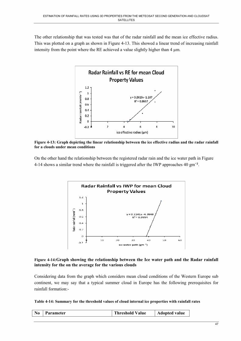
ESTIMATION OF RAINFALL RATES USING 3D PROPERTIES FROM THE METEOSAT SECOND GENERATION AND CLOUDSAT SATELLITES
47
The other relationship that was tested was that of the radar rainfall and the mean ice effective radius. This was plotted on a graph as shown in Figure 4-13. This showed a linear trend of increasing rainfall intensity from the point where the RE achieved a value slightly higher than 4 µm.
Figure 4-13: Graph depicting the linear relationship between the ice effective radius and the radar rainfall for a clouds under mean conditions On the other hand the relationship between the registered radar rain and the ice water path in Figure 4-14 shows a similar trend where the rainfall is triggered after the IWP approaches 40 gmˉ².
Figure 4-14:Graph showing the relationship between the Ice water path and the Radar rainfall intensity for the on the average for the various clouds
Considering data from the graph which considers mean cloud conditions of the Western Europe sub continent, we may say that a typical summer cloud in Europe has the following prerequisites for rainfall formation:- Table 4-14: Summary for the threshold values of cloud internal ice properties with rainfall rates No Parameter Threshold Value Adopted value

ESTIMATION OF RAINFALL RATES USING 3D PROPERTIES FROM THE METEOSAT SECOND GENERATION AND CLOUDSAT SATELLITES
48
1 Ice water path (gmˉ²) 30.147 38
2 Ice Water Content (mgmˉ³) 4.158 4.2
3 Ice Effective Radius (µm) 5.610 5.6 Figure 4-15 shows how the rainfall rates from the weather radars and that from the MSG-MPE products compare considering the mean values of variables of CloudSat referred to in Table 4-14. It illustrates that in most cases the MPE products over-estimates the rainfall as the case for the UK, S. France and S.E Netherlands but may also give a false alarm indicating rain where there isn’t any as for the case in Belgium.
Figure 4-15: Summary of the MSG and radar rainfall rates comparison for all the study sites.
4.4. Statistical Analysis
The following linear regression analysis was done on the independent (radar rainfall) and the three dependent variables (IWC, IWP and RE) Multiple Regressions on Data1: Independent: Column(C) -> Column (E) Dependent: Column (A) Parameter Value Error t-Value Prob>|t| Y-Intercept -0.13431 0.14645 -0.91713 0.35961 α1 -0.05859 0.0066 -8.87466 <0.0001 α2 0.46235 0.04477 10.32786 <0.0001 α3 0.02004 0.02728 0.73445 0.46309 R-Square (COD) Adj. R-Square Root-MSE (SD) 0.31562 0.31065 1.09823 ANOVA Table: Degrees of Item Freedom Squares Square Sum of Mean F Statistic

ESTIMATION OF RAINFALL RATES USING 3D PROPERTIES FROM THE METEOSAT SECOND GENERATION AND CLOUDSAT SATELLITES
49
Model 3 229.72453 76.57484 63.48967 Error 413 498.119 1.2061 Total 416 727.84353 Prob>F 0.0001a The results show an R-square of 0.31562, which is slightly below average for a relatively good relationship, meaning that the algorithm will have a success rate of approximately 32%. This regression analysis which considered all the observed cloud data for various Western European countries, in comparison to the radar rainfall data during the summer seasons of 2007 and 2009. The radar rainfall as a function of IWP, IWC and RE gave the following relationship:- Radar rain = -0.13431+ α1 IWP + α2 IWC + α3 RE Equation 4-1 Replacing the coefficients in Equation 4-1with the values obtained in the statistical analysis we get the following equation
Radar rain= -0.13431+-0.05859 IWP+0.46235 IWC+0.02004 RE Equation 4-2
This is a clear indication that there are other major factors of cloud properties other than just IWC, IWP and RE that may be used to estimate the rainfall rates for areas in Europe. The combined flow chart of algorithm is shown in Figure 4-16. Notice that the above formula only applies with variables possess values equal to or above their thresholds shown in Table 4-14.
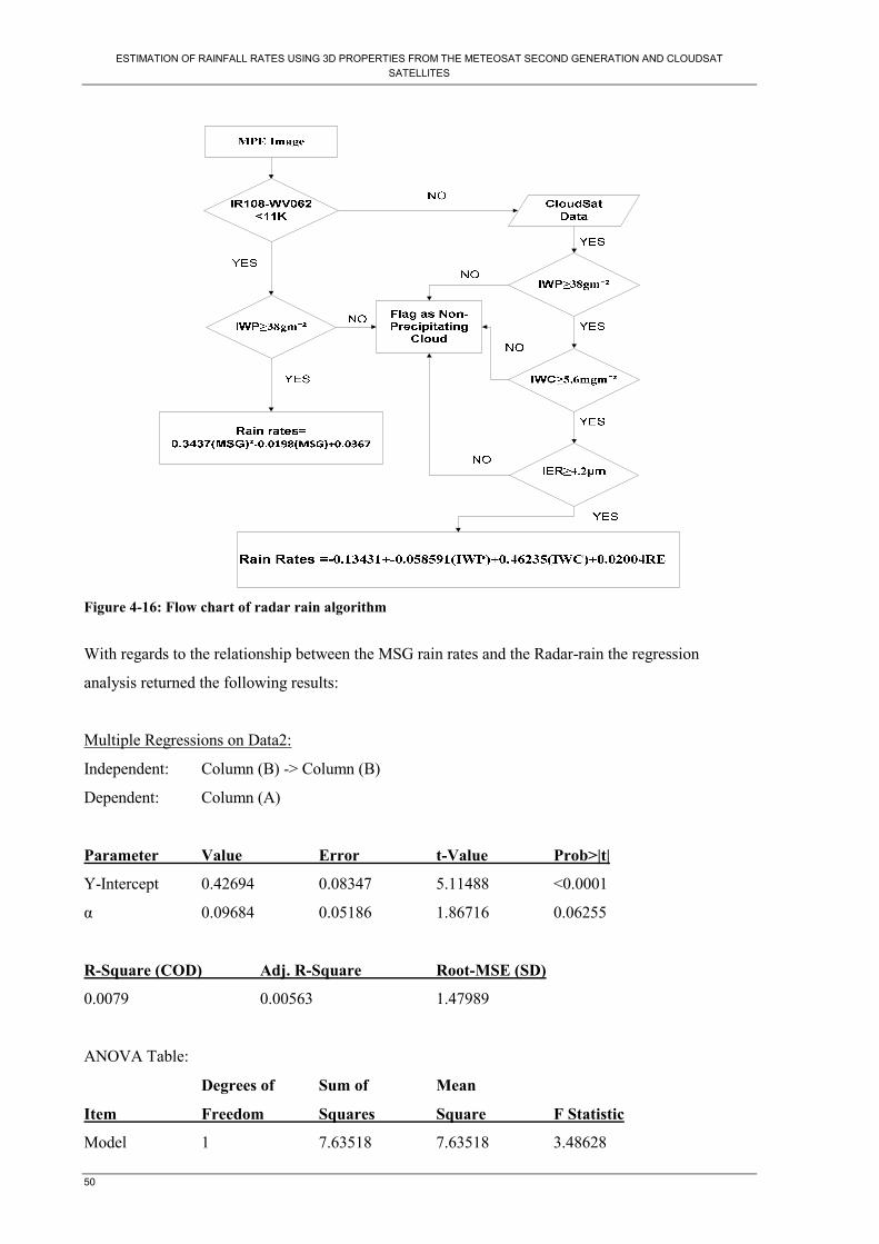
ESTIMATION OF RAINFALL RATES USING 3D PROPERTIES FROM THE METEOSAT SECOND GENERATION AND CLOUDSAT SATELLITES
50
Figure 4-16: Flow chart of radar rain algorithm
With regards to the relationship between the MSG rain rates and the Radar-rain the regression
analysis returned the following results:
Multiple Regressions on Data2:
Independent: Column (B) -> Column (B)
Dependent: Column (A)
Parameter Value Error t-Value Prob>|t|
Y-Intercept 0.42694 0.08347 5.11488 <0.0001
α 0.09684 0.05186 1.86716 0.06255
R-Square (COD) Adj. R-Square Root-MSE (SD)
0.0079 0.00563 1.47989
ANOVA Table:
Degrees of Sum of Mean
Item Freedom Squares Square F Statistic
Model 1 7.63518 7.63518 3.48628

ESTIMATION OF RAINFALL RATES USING 3D PROPERTIES FROM THE METEOSAT SECOND GENERATION AND CLOUDSAT SATELLITES
51
Error 438 959.24879 2.19007
Total 439 966.88398
Prob>F 0.06255
The relationship between the rain radar and the MSG rainfall rates will be given with this relation
Radar rain= 0.42694+0.09684(MSG) Equation 4-3
However this relation generally has a poor R-Square of 0.006255, with a very low success rate.
5. Discussion
5.1. Cloud Ice and Rain Thresholds
It can be concluded that a rainy cloud has to undergo some water and ice droplet accumulation processes before it can produce rain. This is cloud development, where the water droplets condense into super cooled water droplets ice droplets which become heavy enough for the gravitational force to overcome the turbulent winds and drag forces usually present at the high altitudes where the clouds these are located. To enable this to happen, the cloud must achieve a certain concentration of cloud constituents regarding its water amount either in form of ice or liquid) and at the appropriate sizes to trigger precipitation. From the study carried out, it comes out that some of the important cloud properties that may allow it to produce precipitation are adequate
• ice water content • ice effective radius • ice water path
These properties are all in some way correlated to one another, and a substantial decline in any of them affects the others thereby reducing the chances of the clouds ability to yield precipitation. For

ESTIMATION OF RAINFALL RATES USING 3D PROPERTIES FROM THE METEOSAT SECOND GENERATION AND CLOUDSAT SATELLITES
52
instance, high value of IWC but with high RE and but a low IWP may mean that this particular cloud may be a remnant of a cumulonimbus anvil which is full of ice crystals but is too far above and too narrow in the vertical dimension to produce rain. In fact the inclusion of IWP values in the algorithm is vital in the elimination of high cold and icy cirrus clouds from giving false alarms as rainy clouds. Apart from the IWC, IWP and RE, the final relatively below average relationship between them the radar rainfall may be attributed to other factors belonging to the cloud (e.g. LWP in which CloudSat could not measure effectively) and also external factors. One of the sources of error could have been external properties of the clouds like vertical extent and cloud height above ground had not factored in this study. These are factors which are important when describing a cloud genera (Met Office, 2007a).
5.2. Sources of Error
5.2.1. Parallax
One of the major contributors of error in this study when comparing the radar and MPE products could be due to the parallax of the MSG cloud products between the cloud and ground coordinates. CloudSat due to its orientation being always nadir to the PoV does not suffer this shortcoming (Labo et al., 2007). This could have resulted in lack of synchrony between the Radar and CloudSat pixels on one hand, and the MSG pixels on the other hand.
5.2.2. Time Difference
The sensor recording time factor was another cause of error since the sensors were out of synchrony with one another in terms of recording cloud features. This error could have been magnified due to the fluid nature of clouds with the pixels changing in character within a short time
5.2.3. Diverging Liquid Water Measurements
It was observed from the raw data from CloudSat that diverging Liquid water data LWP, RE, LWC which was giving values of- 44.44 was a good indicator of rainy clouds. The lack effective measurement of these important values could have compromised the quality of developed rainfall algorithm. The creation of an algorithm that will effectively measure this important internal property would greatly improve rainfall prediction methods.
5.2.4. Inadequate Tropical Data
When the thresholds were applied to the tropical scenario of the Ewaso Nyiro river Basin in Kenya, it appeared to hold. However, the rain intensities data was missing from the basin and only the daily rainfall totals were relied upon. It was unfortunate that the available Ewaso Nyiro rainfall data’s last recording was done on 3 January 2007 while the first MPE rainfall data begins on 25 December 2006 to date. It was only unfortunate that during this 10 day “window” there was no CloudSat overpasses in the basin to allow a comparison of MPE and CloudSat data. The data from the tropics assisted in

ESTIMATION OF RAINFALL RATES USING 3D PROPERTIES FROM THE METEOSAT SECOND GENERATION AND CLOUDSAT SATELLITES
53
confirming the presence of rainfall when the cloud ice property thresholds were attained, but not by how much.

ESTIMATION OF RAINFALL RATES USING 3D PROPERTIES FROM THE METEOSAT SECOND GENERATION AND CLOUDSAT SATELLITES
54
6. Conclusion and Outlook This chapter outlines the conclusions and recommendations of this study. The study fulfilled the research objectives and answered the research questions as outlined in sections 1.3 and 1.4. The major conclusions of the study are outlined below.
6.1. Research Questions
• How can the rainfall estimates be improved by merging high temporal resolution
Remote Sensing data from MSG with the high spatial resolution Remote Sensing data from CloudSat? This can be done by comparing the pixel information from the MPE rainfall intensity product and the corresponding internal cloud properties from CloudSat using the radar rainfall intensity product as a reference. The thresholds of some of the influencing variables determining the occurrence of rainfall are identified and a simple mathematical relation created.
• How can vertical profile information from CloudSat be merged with integrated profile information from SEVIRI? This was made possible by creating tables of pixel information regarding cloud and rainfall information for identical geographical coordinates and comparing them.
• How do the sensor specifications (viewing angle, pixel size) influence the resultant rainfall rates? There is an inherent parallax error on the MPE products. This error increases on the MSG satellite the closer the clouds move towards the poles. The location coordinates of the cloud top are slightly shifted compare to those of the ground below depending on the satellite zenith angle.
6.2. Research Hypothesis
• Rainfall occurrence can be determined from the internal properties of clouds.
o This hypothesis was proved to be true to some extent. These internal properties were
IWP, RE and IWC.

ESTIMATION OF RAINFALL RATES USING 3D PROPERTIES FROM THE METEOSAT SECOND GENERATION AND CLOUDSAT SATELLITES
55
• Ice particle characteristics within clouds are an important factor in determination of rainfall intensity.
o This was also proved to be true to also some extent, as this study has proved with IWP, RE and IWC where an increase of their respective values enhances the precipitation capabilities of the cloud.
6.3. Conclusion
It can be accepted that cloud properties, both external and internal are important for predicting the amount of rainfall by use of remote sensing based methods. The MSG has the advantage of wide coverage and high temporal of just 15 minutes. On one hand its MPE products give fairly good rainfall intensity estimates where rain-gauges and weather radars are either inadequate or unavailable. In situation like in Africa were the weather radar has not been utilized due to the high operational costs involved, MPE still plays an important role in rainfall intensity analysis. This, can however, be improved by the use of active radar based satellite like CloudSat that can profile through the cloud to assess the existence of internal measurable variables determining conditions favourable for rainfall formation. Even though CloudSat is on an experimental mission, it has proved that a space borne sensor can also be useful, albeit with limitations, to complement ground measurements.
6.4. Outlook
The outlook is that CloudSat, for now may be restricted to a no swath capabilities and narrow Field of View (FoV) due to limitations with battery power and solar panel size and rocket payload capabilities. The dilemma is that increasing the number of batteries and panel size would make the satellite bigger and heavier and thus difficult to place on board a rocket to space. But with the ever advancing technology, it is hoped that in the near future it will be possible to produce more efficient and lighter batteries and panels to allow a bigger swath area and FoV. Also, more CloudSat-like satellite would be launched in space to compensate for the poor current temporal resolution. This study was conducted on the summer months of the Northern Hemisphere, in order to simulate as closest as possible, the tropical climate, since the purpose of the results was its applications in the tropics. It would be interesting if another study would be done for the winter season to incorporate the cloud and snowfall relations. This study encountered some limitation of the data quality from Africa that was used in validation. It is hoped that in the future with the inclusion of rainfall rates and increased data from more stations from the tropics, it will be interesting to establish whether there exists more cloud characteristic thresholds for the tropics since this study used only two data sets consisting of total daily rainfall.
ESTIMATION OF RAINFALL RATES USING 3D PROPERTIES FROM THE METEOSAT SECOND GENERATION AND CLOUDSAT SATELLITES
56
References
Austin, R., 2003. Level 2B Cloud Liquid Water Content Process Description and Interface Control
Document. In: NASA (Editor). Colorado State University.
Austin, R., 2004. Level 2 Cloud Ice Water Content Product Process Description and Control
Document. In: NASA (Editor). Colorado State University, Fort Collins.
Benedetti, A. et al., 2003. Ice Cloud Microphysics Retrievals from Millimetre Radar and Visible
Optical Depth using an Estimation Theory Approach. Geophysics Research, 108(4335).
Cess, R.D. et al., 1989. Interpretation of Cloud-Climate Feedbacks as Produced by 14 General
Circulation Models. Science, 245: 513-516.
EUMETSAT, 2005. MSG-In Orbit-In Use. In: J. Morgan et al. (Editors), Darmstadt, pp. 2-6.
EUMETSAT, 2008. MSG Meteorological Products Extraction Facility Algorithm Specifications
Document. EUMETSAT, Darmstadt, pp. 236-240.
Finnerty, B.D. et al., 1997. Space-time Scale Sensitivity of the Sacramento Model to Radar-gauge
Precipitation Inputs. Journal of Hydrology, 203: 21-38.
Holleman, I., 2007a. Bias Adjustment and Long-term Verification of Radar based Precipitation
Estimates. Meteorological Applications, 14: 195-203.
Holleman, I., 2007b. Intensities from KNMI Radar Data.
IPCC., 2001. The Scientific Basis. In: J.T. Houghton, Ding, Y., Giggs, D. J., (Editor), Climate Change
2001. Cambridge University Press.
Jakob, C. et al., 1999. The Role of Vertically Varying Cloud Fraction in the Parameterization of
Microphysical Processes in the ECMWF model. Quarterly Journal of the Royal Meteorological
Society, 125: 941-965.
Jayakrishnan, R. et al., 2004. Comparison of Rain gauge and WSR-88D Stage III Precipitation Data
over the Texas-Gulf Basin. Journal of Hydrology, 292: 135-152.
Krajewski, W.F. et al., 2002. Radar Hydrology: Rainfall Estimation. Advances in Water Resources,
25: 1387-1394.

ESTIMATION OF RAINFALL RATES USING 3D PROPERTIES FROM THE METEOSAT SECOND GENERATION AND CLOUDSAT SATELLITES
57
Kummerow, C.D. et al., 2001. The Evolution of the Goddard Profiling Algorithm (GPROF) for
Rainfall Estimation from Passive Microwave Sensors. Journal of Applied Meteorology, 40: 1801-
1820.
Labo, E. et al., 2007. The Parallax Correction of MSG Images on the Basis of SAFNWC Cloud top
Height Product. In: H.M. Service (Editor). OMSZ, Budapest.
Legates, D.R. et al., 1993. Precipitation Measurement Biases in the United States, Water Resources
Bulletin, pp. 855-861.
Marshall, J. et al., 1948. The Distribution of Raindrops with Size. Journal of Meteorology, 5: 165-
166.
Menzel, P.W., 2001. Cloud Tracking with Satellite Imagery. Bulletin of the American Meteorological
Society, 82: 33-47.
Met Office, 2007a. Factsheet No. 1- Clouds, National Meteorological Library and Archive. Crown,
pp. 6-18.
Met Office, 2007b. Weather Radar, National Meteorological Library & Archive. Crown Copyright,
Exeter, pp. 11-15.
Nakajima, T. et al., 1990. Determination of the Optical Thickness and Effective Particle Radius of
Clouds from Reflected Solar Radiation Measurements. J. Atmospheric Sciences, 47: 1878-1893.
NASA, 2009. CloudSat. Department of Atmospheric Science, Colorado State University.
Poore, K.D. et al., 1995. Cloud Layer Thickness from a Combination of Surface and Upper-Air
Observations. Journal of Climate, 8: 550-568.
Probert-Jones, J.R., 1962. The Radar Equation in Meteorology. Quarterly Journal of the Royal
Meteorological Society, 88: 486-495.
Rinehart, R.E., 2004. Radar for Meteorologists. Rinehart Publications.
Rossow, W.B. et al., 1999. Advances in Understanding Clouds from ISCCP. Bulletin of the American
Meteorological Society, 80: 2261-2287.
Stephens, G.L. et al., 2002. The CloudSat Mission and the A-train. American Meteorological Society:
1771-1790.

ESTIMATION OF RAINFALL RATES USING 3D PROPERTIES FROM THE METEOSAT SECOND GENERATION AND CLOUDSAT SATELLITES
58
Wang, X. et al., 2007. Validating NEXRAD MPE and Stage III Precipitation Products for
Uniform Rainfall on the Upper Guadalupe River Basin of the Texas Hill Country
Journal of Hydrology, 348: 73-86.
Xie, P. et al., 1995. Analyses of Global monthly Precipitation Using Observations, Satellite Estimates,
and Numerical Weather Predictions. Climate, 9: 840-858.

ESTIMATION OF RAINFALL RATES USING 3D PROPERTIES FROM THE METEOSAT SECOND GENERATION AND CLOUDSAT SATELLITES
59
Appendix
Appendix 1:Ilwis stuff Table 6-1: Summary of the Image Projection used for the KNMI radar image Parameter Value
1 Projection Polar stereographic
2 Projection origin 0E, 90N
3 True scale 60N latitude
4 Pixel size 1 km by 1 km
The values for the rainfall rates in the radar image were derived using the formula R=10^ ((value-109)/32) 6-1 Where R= rainfall rates in mmhˉ¹
Value= the backscatter reflectance value in 8-bit (0 – 255)
The other radar image covers Western Europe and was also in the HDF5 format. The original radar image as projected by the HDF view had the following characteristics.
Appendix 2: Map Projections
KNMI Radar
Group size = 0 Number of attributes = 3 Projection indication = Y projection name = SATELLITE_VIEW projection proj4 params = +proj=geos +a=6378.140 (W-E diameter) +b=6356.755 (N-S diameter) +lat_0=0.0 (latitude at nadir) +lon_0=0.0 (longitude at nadir) +h=35785.86 (height above earth’s surface) +x_0=0 (pixel origin: left hand corner) +y_0=0 (pixel origin: left hand corner)

ESTIMATION OF RAINFALL RATES USING 3D PROPERTIES FROM THE METEOSAT SECOND GENERATION AND CLOUDSAT SATELLITES
60
Geographic (1576) Group size = 1 Number of attributes = 10 Geo number rows = 600 Geo number columns = 800 Geo pixel size x = 2.9986217 Geo pixel size y = -2.9986217 Geo par pixel = X, Y Geo dim pixel = KM, KM Geo column offset = -296.0 Geo row offset = -1668.0 Geo pixel def = LU Geo product corners = -9.640839, 31.384003; -17.735338, 60.108738;
33.11731, 61.38323; 16.681625, 31.558323. OPERA Radar [Ilwis] Description =polar stereographic for radar composite nl25 = Time 1252083524 = Version 3.1 =Class=Coordinate System Projection Type=CoordSystem [Domain] Type=DomainCoord [CoordSystem] CoordBounds=-1e+308 -1e+308 -1e+308 -1e+308 Width=28 Decimals=2 UnitSize=1.000000 Type=Projection Projection=StereoGraphic (Polar) Ellipsoid=International 1924 [Projection] Central Meridian=0.0000000000 Latitude of True Scale=60.0000000000 Central Parallel=90.0000000000 Scale Factor=1.0000000000 Northern Hemisphere=Yes
Appendix 3: Format Overview of CloudSat data Products The CloudSat 2B-LWC Product produces estimates of among other variables, the liquid water content, liquid water path, effective radius, and droplet number density, together with estimated uncertainties in each of these quantities. Supplementary variables indicating the retrieval’s goodness-of-fit, retrieval status, and the influence of a priori data are also included in the output. Data from two retrieval modes are included: a radar-only mode (run for the entire orbit) and a radar + visible optical depth retrieval (run for the daytime side, when optical depth information is available from 2B-TAU).

ESTIMATION OF RAINFALL RATES USING 3D PROPERTIES FROM THE METEOSAT SECOND GENERATION AND CLOUDSAT SATELLITES
61
The format chosen for CloudSat 2B-LWC data is similar to that for CPR Level 2 GEOPROF data. The format consists of metadata, which describes the data characteristics, and swath data, which includes the a priori and forward model inputs, the retrieved quantities, uncertainties, and other information. The variable nray is the number of radar block rays in a granule (orbit). Output fields for quantities not produced during the night-time half of the orbit will be filled with fill values. Each block is a 0.16 s average, based on the average 2B-GEOPROF data from the corresponding period. Time (Vdata data, array size nray, 10-byte integer) Time is determined based on VTCW time. See Table 2 of Li and Durden (2001) for data format. Geolocation (SDS, array size 2 × nray, 4-byte float). As documented in Li and Durden (2001), geolocation is defined as the Earth location of the centre of the IFOV at the altitude of the Earth ellipsoid. The first array dimension is latitude and longitude, in that order. The next dimension is ray number. Values are represented as floating point decimal degrees. Off earth is represented as less than or equal to -9999.9. Latitude is positive north, negative south. Longitude is positive east, negative west. Radar-only (RO) Retrieval RO a priori geometric mean radius (SDS, array size nray, 2-byte integer) A priori value of rg supplied to the RO retrieval algorithm. It ranges from 0 to 100 µm and is multiplied by 100 and stored as a 2-byte integer. The value is selected based on the cloud type and location as obtained from 2B-CLDCLASS. Fill values are CC: 0, UZ: −7777, and CS: −8888. RO a priori std. dev (geometric mean radius) (SDS, array size nray, 2-byte integer) Standard deviation of the a priori value of rg supplied to the RO retrieval algorithm. It ranges from 0 to 100 µm and is multiplied by 100 and stored as a 2-byte integer. The value is selected in the same manner as rg. Fill values are CC: 0, UZ: −7777, and CS: −8888. RO input column droplet number density (SDS, array size nray, 2-byte integer) Fixed value of NT supplied to the RO retrieval algorithm, selected based on cloud type and location as obtained from 2B-CLDCLASS. It ranges from 0 to 3000 cm−3 and is multiplied by 10 and stored as a 2-byte integer. (The RO version of the retrieval does not retrieve NT.) Fill values are CC: 0, UZ: −7777, and CS: −8888. RO input std. dev (column droplet number density) (SDS, array size nray, 2-byte integer) Standard deviation of the input value of NT supplied to the RO retrieval algorithm. It ranges from 0 to 3000 cm−3 and is multiplied by 10 and stored as a 2-byte integer. The value is selected in the same manner as NT. Fill values are CC: 0, UZ: −7777, and CS: −8888.

ESTIMATION OF RAINFALL RATES USING 3D PROPERTIES FROM THE METEOSAT SECOND GENERATION AND CLOUDSAT SATELLITES
62
RO input distribution width parameter (SDS, array size nray, 2-byte integer) Fixed value of _log supplied to the RO retrieval algorithm, selected based on cloud type and location as obtained from 2B-CLDCLASS. It ranges from 0 to 5 (unit less) and is multiplied by 1000 and stored as a 2-byte integer. (The retrieval does not retrieve _log.) Fill values are CC: 0, UZ: −7777, and CS: −8888. RO input std. dev (distribution width parameter) (SDS, array size nray, 2-byte integer) Standard deviation of the input value of _log supplied to the RO retrieval algorithm. It ranges from 0 to 5 (unit less) and is multiplied by 1000 and stored as a 2-byte integer. The value is selected in the same manner as _log. Fill values are CC: 0, UZ: −7777, and CS: −8888. Radar uncertainty (SDS, array size nray, 2-byte integer) Uncertainty in the radar reflectivity factor Ze as obtained from2B-GEOPROF. It ranges from 0 to 100 dBZ and is multiplied by 100 and stored as a 2-byte integer. (TBD: will this be a fixed value for long periods of time, fixed for a position in the orbit, or vary with position in the radar profile?) Fill values are CC: 0, UZ: −7777, and CS: −8888. RO effective radius (SDS, array size nbin × nray, 2-byte integer) RO retrieved profile of effective radius re. It ranges from 0 to 100 µm and is multiplied by 100 and stored as a 2-byte integer. Fill values are CC: 0, NG: −3333, DV: −4444, UZ: −7777, and CS: −8888. RO effective radius uncertainty (SDS, array size nbin × nray, 1-byte unsigned integer) Fractional uncertainty in the RO retrieved re, expressed in percent and rounded to the nearest integer. It ranges from 0 to 250% and is stored as a 1-byte unsigned integer. A value of 250 indicates an uncertainty _ 250%. Fill values are CC: 0, NG: 253, DV: 253, UZ: 253, and CS: 254. RO liquid water content (SDS, array size nbin × nray, 2-byte integer) RO retrieved profile of ` (LWC). It ranges from 0 to 10 g m−3 and is multiplied by 100 and stored as a 2-byte integer. Fill values are CC: 0, NG: −3333, DV: −4444, UZ: −7777, and CS: −8888. RO LWC uncertainty (SDS, array size nbin × nray, 1-byte unsigned integer) Fractional uncertainty in the RO retrieved `, expressed in percent and rounded to the nearest integer. It ranges from 0 to 250% and is stored as a 1-byte unsigned integer. A value of 250 indicates an uncertainty _ 250%. Fill values are CC: 0, NG: 253, DV: 253, UZ: 253, and CS: 254.

ESTIMATION OF RAINFALL RATES USING 3D PROPERTIES FROM THE METEOSAT SECOND GENERATION AND CLOUDSAT SATELLITES
63
RO liquid water path (SDS, array size nray, 2-byte integer) RO retrieved value of W (LWP). It ranges from 0 to 10 kg m−2 and is multiplied by 100 and stored as a 2-byte integer. Fill values are CC: 0, NG: −3333, DV: −4444, UZ:−7777, and CS:−8888. RO LWP uncertainty (SDS, array size nray, 1-byte unsigned integer) Fractional uncertainty in the RO retrieved W, expressed in percent and rounded to the nearest integer. It ranges from 0 to 250% and is stored as a 1-byte unsigned integer. A value of 250 indicates an uncertainty _ 250%. Fill values are CC: 0, NG: 253, DV: 253, UZ: 253, and CS: 254. RO chi-square (SDS, array size nray, 2-byte integer) Goodness-of-fit statistic _2 for the RO retrieved state vector (profile of rg). It ranges from 0 to 100 (unit less) and is multiplied by 100 and stored as a 2-byte integer. Fill values are CC: 0, NG: −3333, DV: −4444, UZ: −7777, and CS: −8888. RO profile dimension (SDS, array size nray, 1-byte integer) Number of elements n in the RO retrieved state vector. It ranges from 0 to 125 and is stored as a 1-byte integer. The retrieval works with measurement and state vectors that are just long enough to hold all the cloudy pixels, as detected by the 2B-GEOPROF algorithm. This length is usually far less than the full n bin-bin radar profile. Fill values are CC: 0, UZ:-77, and CS:-88. RO A matrix diagonal (SDS, array size nbin × nray, 2-byte integer) Diagonal elements of the “averaging kernel” matrix A. It ranges from 0 to 2 (unit less) and is multiplied by 1000 and stored as a 2-byte integer. Fill values are CC: 0, NG: −3333, DV: −4444, UZ: −7777, and CS: −8888.
Appendix 4: Batch Algorithm Batch file for converting radar image into ILWIS format compartible with polar stereographic coordinate system @echo off set longfilename=%1 set shortfilename1=%longfilename:~0,28% "C:\programfiles\FWTools2.4.2\bin\gdal_translate.exe"-of ilwishdf5:% longfilename%://image1 / image_data %longfilename% ren %1 %shortfilename1% "C:\programfiles\52N\ilwis\ilwis.exe"-C d:\thesis\data\GRad\05\%shortfilename1%_ logR.mpr: = ('d:\thesis\data\GRad\05\%shortfilename1%'.mpr-109)/32 "C:\programfiles\52N\ilwis\ilwis.exe" -C d:\thesis\data\GRad\05\%shortfilename1%_R.mpr:= pow(10,'d:\thesis\data\GRad\05\%shortfilename1%_logR'.mpr)
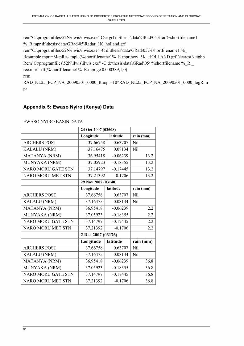
ESTIMATION OF RAINFALL RATES USING 3D PROPERTIES FROM THE METEOSAT SECOND GENERATION AND CLOUDSAT SATELLITES
64
rem"C:\programfiles\52N\ilwis\ilwis.exe"-Csetgrf d:\thesis\data\GRad\05 \frad%shortfilename1 %_R.mpr d:\thesis\data\GRad\05\Radar_1K_holland.grf rem"C:\programfiles\52N\ilwis\ilwis.exe" -C d:\thesis\data\GRad\05\%shortfilename1 %_ Resample.mpr:=MapResample(%shortfilename1%_R.mpr,new_5K_HOLLAND.grf,NearestNeighb Rem"C:\programfiles\52N\ilwis\ilwis.exe" -C d:\thesis\data\GRad\05\ %shortfilename %_R _ rec.mpr:=iff(%shortfilename1%_R.mpr ge 0.000389,1,0) rem RAD_NL25_PCP_NA_20090501_0000_R.mpr=10^RAD_NL25_PCP_NA_20090501_0000_logR.mpr
Appendix 5: Ewaso Nyiro (Kenya) Data
EWASO NYIRO BASIN DATA
24 Oct 2007 (02608) Longitude latitude rain (mm)
ARCHERS POST 37.66758 0.63707 Nil KALALU (NRM) 37.16475 0.08134 Nil MATANYA (NRM) 36.95418 -0.06239 13.2 MUNYAKA (NRM) 37.05923 -0.18355 13.2 NARO MORU GATE STN 37.14797 -0.17445 13.2 NARO MORU MET STN 37.21392 -0.1706 13.2 29 Nov 2007 (03140) Longitude latitude rain (mm)
ARCHERS POST 37.66758 0.63707 Nil KALALU (NRM) 37.16475 0.08134 Nil MATANYA (NRM) 36.95418 -0.06239 2.2 MUNYAKA (NRM) 37.05923 -0.18355 2.2 NARO MORU GATE STN 37.14797 -0.17445 2.2 NARO MORU MET STN 37.21392 -0.1706 2.2 2 Dec 2007 (03176) Longitude latitude rain (mm) ARCHERS POST 37.66758 0.63707 Nil KALALU (NRM) 37.16475 0.08134 Nil MATANYA (NRM) 36.95418 -0.06239 36.8 MUNYAKA (NRM) 37.05923 -0.18355 36.8 NARO MORU GATE STN 37.14797 -0.17445 36.8 NARO MORU MET STN 37.21392 -0.1706 36.8

ESTIMATION OF RAINFALL RATES USING 3D PROPERTIES FROM THE METEOSAT SECOND GENERATION AND CLOUDSAT SATELLITES
65
NARU MORUMETEOROLOGICALSTATION
Day of Event Day of Recording Rainfall in mm
1 20060805 20060806 5 2 20060831 20060901 4.9 3 20060901 20060902 4.9 4 20061021 20061022 7.4 5 20061022 20061023 8.3 6 20061024 20061025 13.2 7 20061025 20061026 30.5 8 20061028 20061029 3.4 9 20061029 20061030 2.2
10 20061031 20061101 7.2 11 20061101 20061102 17.1 12 20061105 20061106 7.4 13 20061107 20061108 22.5 14 20061109 20061110 12.3 15 20061110 20061111 2.8 16 20061111 20061112 3.2 17 20061115 20061116 11.1 18 20061116 20061117 0.3 19 20061119 20061120 7 20 20061120 20061121 0.7 21 20061121 20061122 9.7 22 20061122 20061123 38.4 23 20061129 20061130 10.2 24 20061130 20061201 2.6 25 20061201 20061202 2.6 26 20061202 20061203 36.8 27 20061203 20061204 2.9 28 20061207 20061208 12.2 29 20061210 20061211 2.3 30 20061212 20061213 3.5 31 20061213 20061214 24.7 32 20061219 20061220 3.5 33 20061225 20061226 19.9 34 20061230 20061231 6.9 35 20070103 20070104 16.2

ESTIMATION OF RAINFALL RATES USING 3D PROPERTIES FROM THE METEOSAT SECOND GENERATION AND CLOUDSAT SATELLITES
66
MATANYA NRM
Day of Event
Day of Recording Rainfall in mm
1 20060806 20060805 5 2 20060831 20060901 4.9 3 20060901 20060902 4.9 4 20061021 20061022 7.4 5 20061022 20061023 8.3 6 20061024 20061025 13.2 7 20061025 20061026 30.5 8 20061028 20061029 3.4 9 20061029 20061030 2.2 10 20061031 20061101 7.2 11 20061101 20061102 17.1 12 20061105 20061106 7.4 13 20061107 20061108 22.5 14 20061109 20061110 16 15 20061110 20061111 2.8 16 20061111 20061112 3.2 17 20061115 20061116 11.1 18 20061116 20061117 0.3 19 20061119 20061120 7 20 20061120 20061121 0.7 21 20061121 20061122 9.7 22 20061122 20061123 38.4 23 20061129 20061130 10.2 24 20061130 20061201 2.6 25 20061201 20061202 2.6 26 20061202 20061203 36.8 27 20061203 20061204 2.9 28 20061207 20061208 12.2 29 20061210 20061211 2.3 30 20061212 20061213 3.5 31 20061213 20061214 24.7 32 20061219 20061220 3.5 33 20061226 20061225 19.9 34 20061230 20061231 6.9 35 20070103 20070104 16.2

ESTIMATION OF RAINFALL RATES USING 3D PROPERTIES FROM THE METEOSAT SECOND GENERATION AND CLOUDSAT SATELLITES
67
NARU MORU GATE STATION
Day of Event Day of Recording
Rainfall in mm
1 20060805 20060806 5 2 20060831 20060901 4.9 3 20060901 20060902 4.9 4 20061021 20061022 7.4 5 20061022 20061023 8.3 6 20061024 20061025 13.2 7 20061025 20061026 30.5 8 20061028 20061029 3.4 9 20061029 20061030 2.2 10 20061031 20061101 7.2 11 20061101 20061102 17.1 12 20061105 20061106 7.4 13 20061107 20061108 22.5 14 20061109 20061110 12.3 15 20061110 20061111 2.8 16 20061111 20061112 3.2 17 20061115 20061116 11.1 18 20061116 20061117 0.3 19 20061119 20061120 7 20 20061120 20061121 0.7 21 20061121 20061122 9.7 22 20061122 20061123 38.4 23 20061129 20061130 10.2 24 20061130 20061201 2.6 25 20061201 20061202 2.6 26 20061202 20061203 36.8 27 20061203 20061204 2.9 28 20061207 20061208 12.2 29 20061210 20061211 2.3 30 20061212 20061213 3.5 31 20061213 20061214 24.7 32 20061219 20061220 3.5 33 20061225 20061226 19.9 34 20061230 20061231 6.9 35 20070103 20070104 16.2
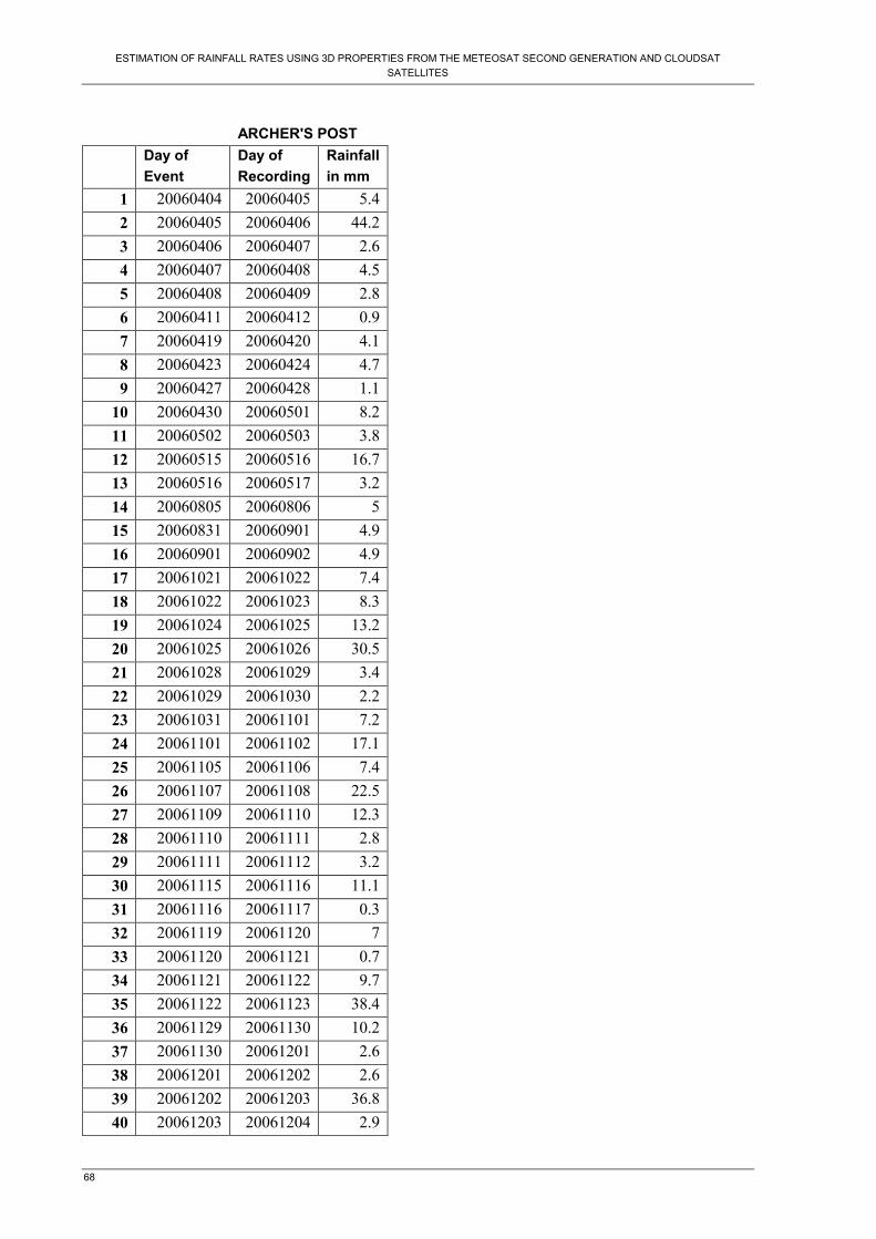
ESTIMATION OF RAINFALL RATES USING 3D PROPERTIES FROM THE METEOSAT SECOND GENERATION AND CLOUDSAT SATELLITES
68
ARCHER'S POST
Day of Event
Day of Recording
Rainfall in mm
1 20060404 20060405 5.4 2 20060405 20060406 44.2 3 20060406 20060407 2.6 4 20060407 20060408 4.5 5 20060408 20060409 2.8 6 20060411 20060412 0.9 7 20060419 20060420 4.1 8 20060423 20060424 4.7 9 20060427 20060428 1.1
10 20060430 20060501 8.2 11 20060502 20060503 3.8 12 20060515 20060516 16.7 13 20060516 20060517 3.2 14 20060805 20060806 5 15 20060831 20060901 4.9 16 20060901 20060902 4.9 17 20061021 20061022 7.4 18 20061022 20061023 8.3 19 20061024 20061025 13.2 20 20061025 20061026 30.5 21 20061028 20061029 3.4 22 20061029 20061030 2.2 23 20061031 20061101 7.2 24 20061101 20061102 17.1 25 20061105 20061106 7.4 26 20061107 20061108 22.5 27 20061109 20061110 12.3 28 20061110 20061111 2.8 29 20061111 20061112 3.2 30 20061115 20061116 11.1 31 20061116 20061117 0.3 32 20061119 20061120 7 33 20061120 20061121 0.7 34 20061121 20061122 9.7 35 20061122 20061123 38.4 36 20061129 20061130 10.2 37 20061130 20061201 2.6 38 20061201 20061202 2.6 39 20061202 20061203 36.8 40 20061203 20061204 2.9

ESTIMATION OF RAINFALL RATES USING 3D PROPERTIES FROM THE METEOSAT SECOND GENERATION AND CLOUDSAT SATELLITES
69
41 20061207 20061208 12.2 42 20061210 20061211 2.3 43 20061212 20061213 3.5 44 20061213 20061214 24.7 45 20061219 20061220 3.5 46 20061225 20061226 19.9 47 20061230 20061231 6.9 48 20070103 20070104 16.2
KALALU NRM
Day of Event Day of Recording Rainfall in mm 1 20060818 20060819 1.9
2 20060820 20060821 0.3
3 20060823 20060824 1.3
4 20060821 20060822 5.5
5 20060825 20060826 4.5
6 20060826 20060827 4
7 20060827 20060828 4.9 8 20060830 20060831 24.6 9 20060831 20060901 8.4
Table 6-2: Summary of table of max value of cloud Properties against corresponding rainfall rates
Place No. of Cloudy bins
No. of Icy Bins
Ice Water Path (gmˉ²)
Liquid Water Path* (Kgmˉ²)
Ice Effective Radius (µm)
Ice Water Content (mgmˉ³)
MSG Rainfall Rates (mmhˉ¹)
Radar Rainfall Rates (mmhˉ¹)
Belgium 33 33 13.8 2.36 6.07 2.08 2.76 0.00 Netherlands 22 15 35.2 7.3 9.38 10.45 0.00 0.60 Netherlands 25 17 8.2 7.18 9.46 3.42 0.00 0.04 Germany 12 5 2.1 7.17 10.02 1.76 0.00 0.17 UK 34 30 213.7 3.02 10.59 32.11 4.16 5.23 France 40 33 217.6 6.5 10.59 32.38 4.64 10.75 France 43 37 157 13.26 9.34 19.81 0.8 N/A Netherlands 35 29 228.2 4.12 8.38 33.97 0.96 1.43 Netherlands 7 5 1.4 8.40 9.12 1.20 0.00 0.00 Germany 5 5 1.8 1.08 6.08 1.50 0.00 0.00 Netherlands 6 6 1.0 0.00 5.62 0.90 0.00 0.00 Netherlands 15 11 2.6 6.55 8.34 0.98 0.00 0.00

ESTIMATION OF RAINFALL RATES USING 3D PROPERTIES FROM THE METEOSAT SECOND GENERATION AND CLOUDSAT SATELLITES
70
Table 6-3: Summary of table of min value of cloud Properties against corresponding rainfall rates
Place No. of Cloudy bins
No. of Icy Bins
Ice Water Path (gm¯²)
Liquid Water Path* (Kgm¯²)
Ice Effective Radius (µm)
Ice Water Content (mgm¯³)
MSG Rainfall Rates (mmh¯¹)
Radar Rainfall Rates (mmh¯¹)
Belgium 13 13 1.80 0.07 4.99 0.43 0.00 0.00 Netherlands 0 0 0.00 0.00 0.00 0.00 0.00 0.00 Netherlands 0 0 0.00 0.00 0.00 0.00 0.00 0.00 Germany 0 0 0.00 0.00 0.00 0.00 0.00 0.00 UK 0 0 0.00 0.00 0.00 0.00 0.00 0.00 S. France 0 0 0.00 0.00 0.00 0.00 0.00 0.03 N. France 2 0 0.00 0.00 0.00 0.00 0.00 N/A Netherlands 1 1 0.00 0.00 4.46 0.30 0.00 0.00 Netherlands 0 0 0.00 0.00 0.00 0.00 0.00 0.00 Germany 0 0 0.00 0.00 0.00 0.00 0.00 0.00 Netherlands 0 0 0.00 0.00 0.00 0.00 0.00 0.00 Netherlands 0 0 0.00 0.00 0.00 0.00 0.00 0.00

ESTIMATION OF RAINFALL RATES USING 3D PROPERTIES FROM THE METEOSAT SECOND GENERATION AND CLOUDSAT SATELLITES
71