Search and Game Playing

1

Overview

• Search problems: definition

• Example: 8-puzzle

• General search

• Evaluation of search strategies

• Strategies: breadth-first, uniform-cost, depth-first

• More uninformed search: depth-limited, iterative deepening,

bidirectional search

2

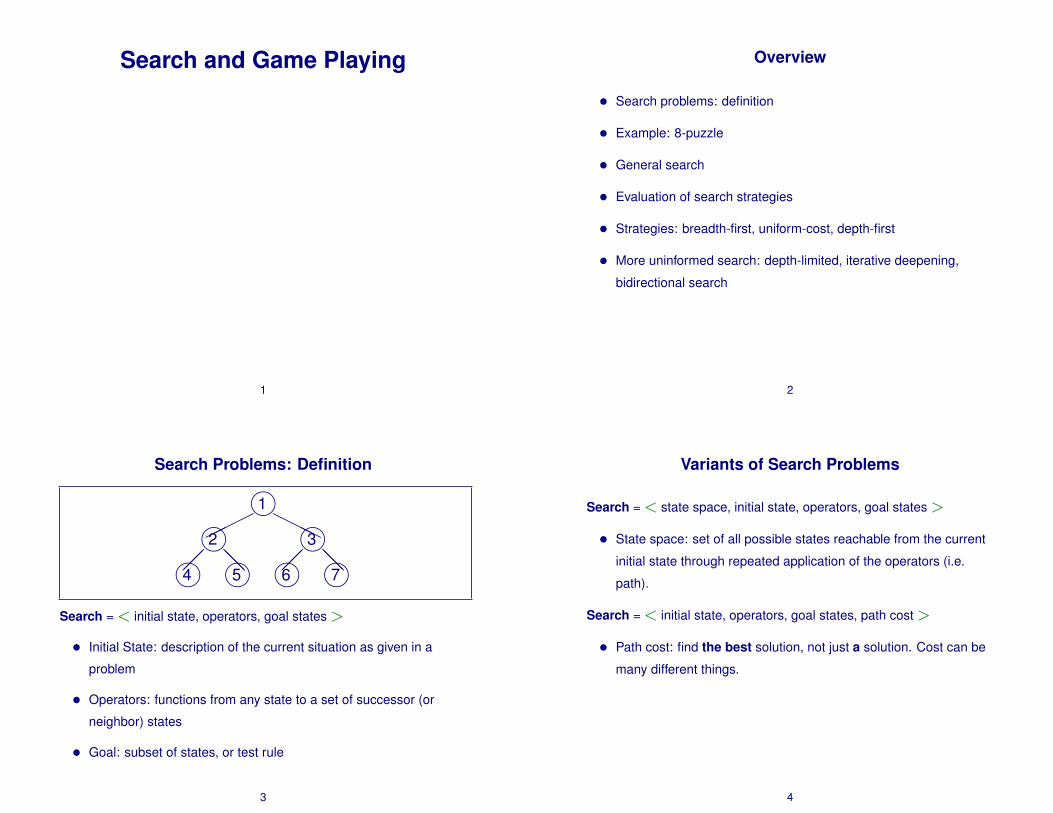
Search Problems: Definition

���HHH

k1�� @@

k2�� @@

k3k4 k5 k6 k7Search =< initial state, operators, goal states>

• Initial State: description of the current situation as given in a

problem

• Operators: functions from any state to a set of successor (or

neighbor) states

• Goal: subset of states, or test rule

3

Variants of Search Problems

Search =< state space, initial state, operators, goal states>

• State space: set of all possible states reachable from the current

initial state through repeated application of the operators (i.e.

path).

Search =< initial state, operators, goal states, path cost>

• Path cost: find the best solution, not just a solution. Cost can be

many different things.

4

Types of Search

���HHH

k1�� @@

k2�� @@

k3k4 k5 k6 k7• Uninformed: systematic strategies (Chapter 3)

• Informed: Use domain knowledge to narrow search (Chapter 4)

• Game playing as search: minimax, state pruning, probabilistic

games (Chapter 5).

5

Search State

State as Data Structure

• examples: variable assignment, properties, order in list, bitmap,

graph (vertex and edges)

• captures all possible ways world could be

• typically static, discrete (symbolic), but doe snot have to be

Choosing a Good Representation

• concise (keep only the relevant features)

• explicit (easy to compute when needed)

• embeds constraints

6

Operators

Function from state to subset of states

• drive to neighboring city

• place piece on chess board

• add person to meeting schedule

• slide tile in 8-puzzle

Characteristics

• often requires instantiation (fill in variables)

• encode constraints (only certain operations are allowed)

• generally discrete: continuous parameters→ infinite branching

7

Goals: Subset of states or test rules

Specification:

• set of states: enumerate the eligible states

• partial description: e.g. a certain variable has value over x.

• constraints: or set of constraints. Hard to enumerate all states

matching the constraints, or very hard to come up with a solution

at all (i.e. you can only verify it; P vs. NP).

Other considerations:

• space, time, quality (exact vs. approximate trade-offs)

8

An Example: 8-Puzzle

5 4

6 1 8

7 3 2

→ ... ↑ ...← ... ↓1 2 3

8 4

7 6 5

• State: location of 8 number tiles and one blank tile

• Operators: blank moves left, right, up, or down

• Goal test: state matches the configuration on the right (see

above)

• Path cost: each step cost 1, i.e. path length, or search tree depth

Generalization: 15-puzzle, ..., (N2 − 1)-puzzle

9

8-Puzzle: Example

2 3

1 8 4

7 6 5

↓1 2 3

8 4

7 6 5

→1 2 3

8 4

7 6 5

Possible state representations in LISP (0 is the blank):

• (0 2 3 1 8 4 7 6 5)

• ((0 2 3) (1 8 4) (7 6 5))

• ((0 1 7) (2 8 6) (3 4 5))

• or use the make-array, aref functions.

How easy to: (1) compare, (2) operate on, and (3) store (i.e. size).

10

8-Puzzle: Search Tree

2 3

1 8 4

7 6 5

↓1 2 3

8 4

7 6 5

→2 3

1 8 4

7 6 5

→1 2 3

8 4

7 6 5

↓1 2 3

7 8 4

6 5

→2 3

1 8 4

7 6 5

↓2 8 3

1 4

7 6 5

GOAL! ... ... ...

11

Goal Test

As simple as a single LISP call:

* (defvar *goal-state* ’(1 2 3 8 0 4 7 6 5))

*GOAL-STATE*

* (equal *goal-state* ’(1 2 3 8 0 4 7 6 5))

T

12

General Search Algorithm

Pseudo-code:

function General-Search (problem, Que-Fn)

node-list := initial-state

loop begin

// fail if node-list is empty

if Empty(node-list) then return FAIL

// pick a node from node-list

node := Get-First-Node(node-list)

// if picked node is a goal node, success!

if (node == goal) then return as SOLUTION

// otherwise, expand node and enqueue

node-list := Que-Fn(node-list, Expand(node))

loop end

13

Evaluation of Search Strategies

• time-complexity: how many nodes expanded so far?

• space-complexity: how many nodes must be stored in node-list at

any given time?

• completeness: if solution exists, guaranteed to be found?

• optimality: guaranteed to find the best solution?

14

Breadth First Search

���HHH

m1�� @@

m2�� @@

m3�� AA

m4�� AA

m5�� AA

m6�� AA

m7m8 m9 m10 m11 m12 m13 m14 m15

• node visit order (goal test): 1 2 3 4 5 6 7 8 9 10 11 12 13 14 15

• queuing function: enqueue at end (add expanded node at the end

of the list)

15

BFS: Expand Order

���HHH

m1�� @@

m2�� @@

m3�� AA

m4�� AA

m5�� AA

m6�� AA

m7m8 m9 m10 m11 m12 m13 m14 m15

Evolution of the queue (bold= expanded and added children):

1. [1] : initial state

2. [2][3] : dequeue 1 and enqueue 2 and 3

3. [3][4][5] : dequeue 2 and enqueue 4 and 5

4. [4][5][6][7] : all depth 3 nodes

...

8. [8][9][10][11][12][13][14][15] : all depth 4 nodes16

BFS: Evaluation

branching factor b, depth of solution d:

• complete: it will find the solution if it exists

• time: 1 + b+ b2 + ...+ bd

• space: O(bd+1) where d is the depth of the shallowest solution

• space is more problem than time in most cases (p 75, figure 3.12).

• time is also a major problem nonetheless (same as time)

17

Uniform Cost

BFS with expansion of lowest-cost nodes: path cost is g(node).

• BFS: g(n) = Depth(node)

18

Depth First Search

���HHH

m1�� @@

m2�� @@

m3�� AA

m4�� AA

m5�� AA

m6�� AA

m7m8 m9 m10 m11 m12 m13 m14 m15

• node visit order (goal test): 1 2 4 8 9 5 10 11 3 6 12 13 7 14 15

• queuing function: enqueue at left (stack push; add expanded

node at the beginning of the list)

19

DFS: Expand Order

���HHH

m1�� @@

m2�� @@

m3�� AA

m4�� AA

m5�� AA

m6�� AA

m7m8 m9 m10 m11 m12 m13 m14 m15

Evolution of the queue (bold=expanded and added children):

1. [1] : initial state

2. [2][3] : pop 1 and push expanded in the front

3. [4][5][3] : pop 2 and push expanded in the front

4. [8][9][5][3] : pop 4 and push expanded in the front

20

DFS: Evaluation

branching factor b, depth of solutions d, max depthm:

• incomplete: may wander down the wrong path

• time: O(bm) nodes expanded (worst case)

• space: O(bm) (just along the current path)

• good when there are many shallow goals

• bad for deep or infinite depth state space

21

Implementation

• Use of stack or queue : explicit storage of expanded nodes

• Recursion : implicit storage in the recursive call stack

22

Key Points

• Description of a search problem: initial state, goals, operators,

etc.

• Considerations in designing a representation for a state

• Evaluation criteria

• BFS, UCS, DFS: time and space complexity, completeness

• Differences and similarities between BFS and UCS

• When to use one vs. another

• Node visit orders for each strategy

• Tracking the stack or queue at any moment

23

Depth Limited Search (DLS): Limited Depth DFS

���HHH

k1�� @@

k2�� @@

k3k4 k5 k6 k7• node visit order for each depth limit l:

1 (l = 1); 1 2 3 (l = 2); 1 2 4 5 3 6 7 (l = 3);

• queuing function: enqueue at front (i.e. stack push)

• push the depth of the node as well:

(<depth><node>)

24

DLS: Expand Order

���HHH

k1�� @@

k2�� @@

k3k4 k5 k6 k7Evolution of the queue (bold=expanded and then added):

(<depth>,<node>)); Depth limit = 3

1. [(d1,1)] : initial state

2. [(d2,2)][(d2,3)] : pop 1 and push 2 and 3

3. [(d3,4)][(d3,5)][(d2,3)] : pop 2 and push 4 and 5

4. [(d3,5)][(d2,3)]: pop 4, cannot expand it further

5. [(d2,3)]: pop 5, cannot expand it further

6. [(d3,6)][(d3,7)]: pop 3, and push 6, 7

...25

DLS: Evaluation

branching factor b, depth limit l, depth of solution d:

• complete: if l ≥ d

• time: O(bl) nodes expanded (worst case)

• space: O(bl) (same as DFS, where l = m (m: max depth of

tree in DFS)

• good if solution is within the limited depth.

• non-optimal (same problem as in DFS).

26

Iterative Deepening Search: DLS by Increasing Limit

���HHH

m1�� @@

m2�� @@

m3�� AA

m4�� AA

m5�� AA

m6�� AA

m7m8 m9 m10 m11 m12 m13 m14 m15

• node visit order:

1 ; 1 2 3; 1 2 4 5 3 6 7; 1 2 4 8 9 5 10 11 3 6 12 13 7 14 15; ...

• revisits already explored nodes at successive depth limit

• queuing function: enqueue at front (i.e. stack push)

• push the depth of the node as well: (<depth><node>)

27

IDS: Expand Order

���HHH

k1�� @@

k2�� @@

k3k4 k5 k6 k7Basically the same as DLS: Evolution of the queue (bold=expanded

and then added): (<depth>,<node>)); e.g. Depth limit = 3

1. [(d1,1)] : initial state

2. [(d2,2)][(d2,3)] : pop 1 and push 2 and 3

3. [(d3,4)][(d3,5)][(d2,3)] : pop 2 and push 4 and 5

4. [(d3,5)][(d2,3)]: pop 4, cannot expand it further

5. [(d2,3)]: pop 5, cannot expand it further

6. [(d3,6)][(d3,7)]: pop 3, and push 6, 7

...28

IDS: Evaluation

branching factor b, depth of solution d:

• complete: cf. DLS, which is conditionally complete

• time: O(bd) nodes expanded (worst case)

• space: O(bd) (cf. DFS and DLS)

• optimal!: unlike DFS or DLS

• good when search space is huge and the depth of the solution is

not known (*)

29

Bidirectional Search (BDS)

GoalStart

• Search from both initial state and goal to reduce search depth.

• O(bd/2) of BDS vs.O(bd+1) of BFS.

30

BDS: Considerations

GoalStart

1. how to back trace from the goal?

2. successors and predecessors: are operations reversible?

3. are goals explicit?: need to know the goal to begin with

4. check overlap in two branches

5. BFS? DFS? which strategy to use? Same or different?

31

BDS Example: 8-Puzzle

5 4

6 1 8

7 3 2

→5 4 8

6 1

7 3 2

→ ...←1 2 3

8 4

7 6 5

←1 2 3

8 4

7 6 5

• Is it a good strategy?

• What about Chess? Would it be a good strategy?

• What kind of domains may be suitable for BDS?

32

Avoiding Repeated States

C

D

B

A

D D D D

C C

B

D D D D

C C

B

A

Repeated states can be devastating in search problems.

• Common cases: problems with reversible operators→ search

space becomes infinite

• One approach: find a spanning tree of the graph

33

Avoiding Repeated States: Strategies

5 4

6 1 8

7 3 2

→5 4 8

6 1

7 3 2

→5 4

6 1 8

7 3 2

→5 4 8

6 1

7 3 2

...

• Do not return to the node’s parent

• Avoid cycles in the path (this is a huge theoretical problem in its

own right)

• Do not generate states that you generated before: use a hash

table to make checks efficient

How to avoid storing every state? Would using a short signature (or a

checksum) of the full state description help?

34

Key Points

• DLS, IDS, BDS search order, expansions, and queuing

• DLS, IDS, BDS evaluation

• DLS, IDS, BDS: suitable domains

• Repeated states: why removing them is important

35

Overview

• Best-first search

• Heuristic function

• Greedy best-first search

• A∗

• Designing good heuristics

• IDA∗

• Iterative improvement algorithms

1. Hill-climbing

2. Simulated annealing

36

Informed Search (Chapter 4)

From domain knowledge, obtain an evaluation function.

• best-first search: order nodes according to the evaluation function

value

• greedy search: minimize estimated cost for reaching the goal –

fast, but incomplete and non-optimal.

• A∗: minimize f(n) = g(n) + h(n), where g(n) is the

current path cost from start to n, and h(n) is the estimated cost

from n to goal.

37

Best First Search

function Best-First-Search (problem, Eval-Fn)

Queuing-Fn← sorted list by Eval-Fn(node)

return General-Search(problem, Queuing-Fn)

• The queuing function queues the expanded nodes, and sorts it

every time by the Eval-Fn value of each node.

• One of the simplest Eval-Fn: estimated cost to reach the goal.

38

Heuristic Function

AB

CE

I

H

G

F

D

• h(n) = estimated cost of the cheapest path from the state at

node n to a goal state.

• The only requirement is the h(n) = 0 at the goal.

• Heuristics means “to find” or “to discover”, or more technically,

“how to solve problems” (Polya, 1957).

39

Heuristics: Example

Straight Line Distance

START

GOAL

AB

CE

I

H

G

F

D

• hSLD(n): straight line distance (SLD) is one example.

• Start from A and Goal is I: C is the most promising next step in

terms of hSLD(n), i.e. h(C) < h(B) < h(F )

• Requires some knowledge:

1. coordinates of each city

2. generally, cities toward the goal tend to have smaller SLD.

40

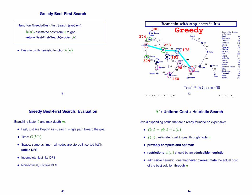
Greedy Best-First Search

function Greedy-Best-First Search (problem)

h(n)=estimated cost from n to goal

return Best-First-Search(problem,h)

• Best-first with heuristic function h(n)

41

� ��� ��� ��� �� � ������ ������ � ��� ���

Bucharest

Giurgiu

Urziceni

Hirsova

Eforie

NeamtOradea

Zerind

Arad

Timisoara

LugojMehadia

DobretaCraiova

Sibiu

Fagaras

PitestiRimnicu Vilcea

Vaslui

Iasi

Straight−line distanceto Bucharest

0160242161

77151

241

366

193

178

253329

80199

244

380

226

234

374

98

Giurgiu

UrziceniHirsova

Eforie

Neamt

Oradea

Zerind

Arad

Timisoara

Lugoj

Mehadia

DobretaCraiova

Sibiu Fagaras

Pitesti

Vaslui

Iasi

Rimnicu Vilcea

Bucharest

71

75

118

111

70

75120

151

140

99

80

97

101

211

138

146 85

90

98

142

92

87

86

���������! "$#&%('*)+,�!-/.&021/-43�.&'/'/%5 $ &026&#�78%(-/%51:9�;21/<!"$=&>&?5@A@2B C4D&02EF-G%(1IHF>J�!% ) -/"$;26&'K?MLJN!>2H O

Total Path Cost = 450

Greedy

329

253178

193

160

98

380

374

42

Greedy Best-First Search: Evaluation

Branching factor b and max depthm:

• Fast, just like Depth-First-Search: single path toward the goal.

• Time: O(bm)

• Space: same as time – all nodes are stored in sorted list(!),

unlike DFS

• Incomplete, just like DFS

• Non-optimal, just like DFS

43

A∗: Uniform Cost + Heuristic Search

Avoid expanding paths that are already found to be expensive:

• f(n) = g(n) + h(n)

• f(n) : estimated cost to goal through node n

• provably complete and optimal!

• restrictions: h(n) should be an admissible heuristic

• admissible heuristic: one that never overestimate the actual cost

of the best solution through n

44

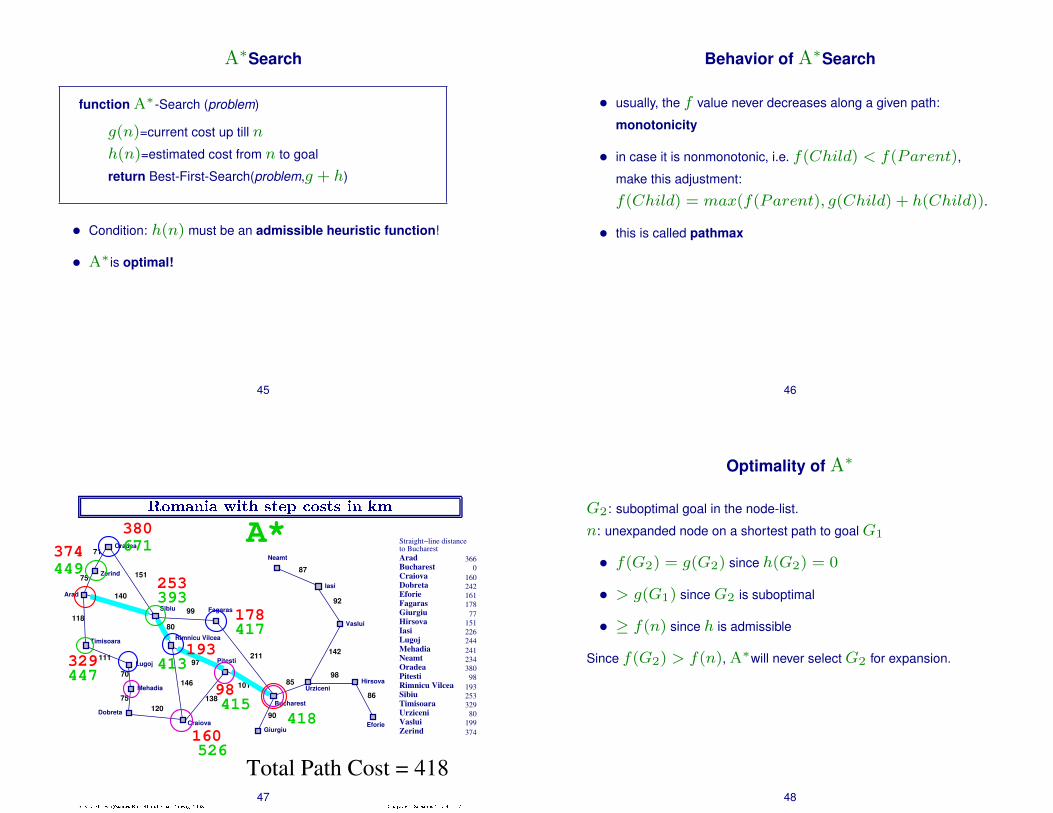
A∗Search

function A∗-Search (problem)

g(n)=current cost up till n

h(n)=estimated cost from n to goal

return Best-First-Search(problem,g + h)

• Condition: h(n) must be an admissible heuristic function!

• A∗ is optimal!

45

Behavior of A∗Search

• usually, the f value never decreases along a given path:

monotonicity

• in case it is nonmonotonic, i.e. f(Child) < f(Parent),

make this adjustment:

f(Child) = max(f(Parent), g(Child) + h(Child)).

• this is called pathmax

46

� ��� ��� ��� �� � ������ ������ � ��� ���

Bucharest

Giurgiu

Urziceni

Hirsova

Eforie

NeamtOradea

Zerind

Arad

Timisoara

LugojMehadia

DobretaCraiova

Sibiu

Fagaras

PitestiRimnicu Vilcea

Vaslui

Iasi

Straight−line distanceto Bucharest

0160242161

77151

241

366

193

178

253329

80199

244

380

226

234

374

98

Giurgiu

UrziceniHirsova

Eforie

Neamt

Oradea

Zerind

Arad

Timisoara

Lugoj

Mehadia

DobretaCraiova

Sibiu Fagaras

Pitesti

Vaslui

Iasi

Rimnicu Vilcea

Bucharest

71

75

118

111

70

75120

151

140

99

80

97

101

211

138

146 85

90

98

142

92

87

86

���������! "$#&%('*)+,�!-/.&021/-43�.&'/'/%5 $ &026&#�78%(-/%51:9�;21/<!"$=&>&?5@A@2B C4D&02EF-G%(1IHF>J�!% ) -/"$;26&'K?MLJN!>2H O

393

447

417

413

415

526

418

671449

Total Path Cost = 418

A*

178

160

98

253

329193

380374

47

Optimality of A∗

G2: suboptimal goal in the node-list.

n: unexpanded node on a shortest path to goalG1

• f(G2) = g(G2) since h(G2) = 0

• > g(G1) sinceG2 is suboptimal

• ≥ f(n) since h is admissible

Since f(G2) > f(n), A∗will never selectG2 for expansion.

48

Optimality of A∗: Example

AB

CE

I

H

G

F

D

1. Expansion of parent allowed: search fails at nodes B, D, and E.

2. Expansion of parent disallowed: paths through nodes B, D,

and E with have an inflated path cost g(n), thus will become

nonoptimal.

A→ C → E → C →︸ ︷︷ ︸inflated path cost

A→ F → ...

49

Lemma to Optimality of A∗

Lemma: A∗expands nodes in order of increasing f(n) value.

• Gradually adds f-contours of nodes (cf. BFS adds layers).

• The goal state may have a f value: let’s call it f∗

• This means that all nodes with f < f∗ will be expanded!

50

Complexity of A∗

A∗ is complete and optimal, but space complexity can become

exponential if the heuristic is not good enough.

• condition for subexponential growth:

|h(n)− h∗(n)| ≤ O(logh∗(n)),

where h∗(n) is the true cost from n to the goal.

• that is, error in the estimated cost to reach the goal should be less

than even linear, i.e.< O(h∗(n)).

Unfortunately, with most heuristics, error is at least proportional with

the true cost, i.e.≥ O(h∗(n)) > O(logh∗(n)).

51

Linear vs. Logarithmic Growth Error

0

2

4

6

8

10

1 2 3 4 5 6 7 8 9 10

xlog(x)

• Error in heuristic: |h(n)− h∗(n)|.• For most heuristics, the error is at least linear.

• For A∗to have subexponential growth, the error in the heuristic

should be on the order ofO(logh∗(n)).

52

Problem with A∗

Space complexity is usually exponential!

• we need a memory bounded version

• one solution is: Iterative Deepening A∗, or IDA∗

53

A∗: Evaluation

• Complete : unless there are infinitely many nodes with

f(n) ≤ f(G)

• Time complexity: exponential in (relative error in h× length of

solution)

• Space complexity: same as time (keep all nodes in memory)

• Optimal

54

Heuristic Functions: Example

Eight puzzle

5 4

6 1 8

7 3 2

1 2 3

8 4

7 6 5

• h1(n) = number of misplaced tiles

• h2(n) = total Manhattan distance (city block distance)

h1(n) = 7 (not counting the blank tile)

h2(n) = 2+3+3+2+4+2+0+2 = 18

* Both are admissible heuristic functions.

55

Dominance

If h2(n) ≥ h1(n) for all n and both are admissible, then we say that

h2(n) dominates h1(n), and is better for search.

Typical search costs for depth d = 14:

• Iterative Deepening : 3,473,941 nodes expanded

• A∗(h1): 539 nodes

• A∗(h2): 113 nodes

Observe that in A∗, every node with f < f∗ is expanded. Since

f = g + h, nodes with h(n) < f∗ − g(n) will be expanded, so

larger h will result in less nodes being expanded.

• f∗ is the f value for the optimal solution path.

56

Designing Admissible Heuristics

Relax the problem to obtain an admissible heuristics.

For example, in 8-puzzle:

• allow tiles to move anywhere→ h1(n)

• allow tiles to move to any adjacent location→ h2(n)

For traveling:

• allow traveler to travel by air, not just by road: SLD

57

Other Heuristic Design

• Use composite heuristics: h(n) = max(h1(n), ..., hm(n))

• Use statistical information: random sample h and true cost to

reach goal. Find out how often h and true cost is related.

58

Iterative Deepening A∗: IDA∗

A∗ is complete and optimal, but the performance is limited by the

available space.

• Basic idea: only search within a certain f bound, and gradually

increase the f bound until a solution is found.

• More on IDA∗ next time.

59

IDA∗

function IDA∗(problem)

root← Make-Node(Initial-State(problem))

f-limit← f-Cost(root)

loop do

solution, f-limit← DFS-Contour(root, f-limit)

if solution != NULL then return solution

if f-limit ==∞ then return failure

end loop

Basically, iterative deepening depth-first-search with depth defined as

the f -cost (f = g + n):

60

DFS-Contour(root, f-limit)

Find solution from node root, within the f -cost limit of f-limit.

DFS-Contour returns solution sequence and new f -cost limit.

• if f -cost(root)> f-limit, return fail.

• if root is a goal node, return solution and new f -cost limit.

• recursive call on all successors and return solution and

minimum f -limit returned by the calls

• return null solution and new f -limit by default

Similar to the recursive implementation of DFS.

61

IDA∗: Evaluation

• complete and optimal (with same restrictions as in A∗)

• space: proportional to longest path that it explores (because it is

depth first!)

• time: dependent on the number of different values h(n) can

assume.

62

IDA∗: Time Complexity

Depends on the heuristics:

• small number of possible heuristic function values→ small

number of f -contours to explore→ becomes similar to A∗

• complex problems: each f -contour only contain one new node

if A∗expandsN nodes,

IDA∗expands

1 + 2 + ..+N =N(N+1)

2= O(N2)

• a possible solution is to have a fixed increment ε for the f -limit

→ solution will be suboptimal for at most ε (ε-admissible)

63

Other Methods: Beam Search

Best-first search with a fixed limited branching factor

• expand the first n nodes with the best Eval-Fn value, where n is

a small number.

• n is called the width of the beam

• good for domains with continuous time functions (like speech

recognition)

• good for domains with huge branching factor (like above)

64

Iterative Improvement Algorithms

Start with a complete configuration (all variable values assigned, and

optimal), andgradually improve it.

• Hill-climbing (maximize cost function)

• Gradient descent (minimize cost function)

• Simulated Annealing (probabilistic)

65

Hill-Climbing

• no queue, keep only the best node

• greedy, no back-tracking

• good for domains where all nodes are solutions:

– goal is to improve quality of the solution

– optimization problems

• note that it is different from greedy search, which keeps a node list

66

Hill-Climbing Strategies

Problems of local maxima, plateau, and ridges:

• try random-restart: move to a random location in the landscape

and restart search from there

• keep n best nodes (beam search) *

• parallel search

• simulated annealing *

Hardness of problem depends on the shape of the landscape.

*: coming up next

67

Hill-Climbing: Problems

30 ft20 ft

10 ft

local maxima plateau

Ridge Slow approach toward max

• Possible solution: simulated annealing – gradually decrease

randomness of move to attain globally optimal solution (more on this

next week).

68

Simulated Annealing: Overview

Annealing:

• heating metal to a high-temperature (making it a liquid) and then

allowing to cool slowly (into a solid); this relieves internal stresses

and results in a more stable, lower-energy state in the solid.

• at high temperature, atoms move actively (large distances with

greater randomness), but as temperature is lowered, they become

more static.

Simulated annealing is similar:

• basically, hill-climbing with randomness that allows going down

as well as the standard up

• randomness (as temperature) is reduced over time

69

Simulated Annealing (SA)

Goal: minimize the energyE, as in statistical thermodynamics.

For successors of the current node,

• if ∆E ≤ 0, the move is accepted

• if ∆E > 0, the move is accepted with probability

P (∆E) = e−∆EkT , where k is the Boltzmann constant and T

is temperature.

• randomness is in the comparison: P (∆E) < rand(0, 1)

∆E = Enew − Eold.

The heuristic h(n) or f(n) representsE.

70

Temperature and P (∆E) < rand(0, 1)

00.10.20.30.40.50.60.70.80.91

0 2 4 6 8 10

T=1T=5

T=10

Downward moves of any size are allowed at high temperature, but at

low temperature, only small downward moves are allowed.

• Higher temperature T → higher probability of downward

hill-climbing

• Lower ∆E→ higher probability of downward hill-climbing

71

T Reduction Schedule

High to low temperature reduction schedule is important:

• reduction too fast: suboptimal solution

• reduction too slow: wasted time

• question: does the form of the reduction schedule curve matter?

linear, quadratic, exponential, etc.?

The proper values are usually found experimentally.

72

Simulated Annealing Applications

• VLSI wire routing and placement

• Various scheduling optimization tasks

• Traffic control

• Neural network training

• etc.

73

Constraint Satisfaction Search

Constraint Satisfaction Problem (CSP):

• state: values of a set of variables

• goal: test if a set of constraints are met

• operators: set values of variables

• general search can be used, but specialized solvers for CSP work

better

74

Constraints

• Unary, binary, and higher order constraints: how many variables

should simultaneously meet the constraint

• Absolute constraints vs. preference constraints

• Variables are defined in a certaindomain, which determines the

possible set of values, either discrete or continuous.

This is part of a much more complex problem called constrained

optimization problems in operations research consisting of cost

function (either minimize or maximize) and several constraints.

Problems can be linear, nonlinear, convex, nonconvex, etc.

Straight-forward solutions exist for a limited subclass of these (for

example, for linear programming problems can be solved by the

simplex method).

75

CSP: continued

• CSPs include NP-complete problems such as 3-SAT, thus finding

the solutions can require exponential time.

• However, constraints can help narrow down the possible options,

therefore reducing the branching factor. This is because in CSP,

the goal can be decomposed into several constraints, rather than

being a whole solution.

• Strategies: backtracking (back up when constraint is violated),

forward checking (do not expand further if look-ahead returns a

constraint violation). Forward checking is often faster and simple

to implement.

76

Heuristics for Constraint Satisfaction Problems

General strategies for variable selection:

• Most-constrained-variable heuristic (var with fewest possible

values)

• Most-constraining-variable heuristic (var involved in the largest

number of constraints)

and for value assignment:

• Least-constraining-value heuristic (value that rules out the

smallest number of values for vars)

Reducing branching factor vs. leaving freedom for future choices.

77

Key Points

• best-first-search: definition

• heuristic function h(n): what it is

• greedy search: relation to h(n) and evaluation. How it is different

from DFS (time complexity, space complexity)

• A∗: definition, evaluation, conditions of optimality

• complexity of A∗: relation to error in heuristics

• designing good heuristics: several rule-of-thumbs

• IDA∗: evaluation, time and space complexity (worst case)

• beam search concept

• hill-climbing concept and strategies

• simulated annealing: core algorithm, effect of T and ∆E, source

of randomness.

• constraint satisfaction search: what kind of domains? why

important?

78

Game Playing

79

Game Playing

• attractive AI problem because it is abstract

• one of the oldest domains in AI

• in most cases, the world state is fully accessible

• computer representation of the situation can be clear and exact

• challenging: uncertainty introduced by the opponent and the

complexity of the problem (full search is impossible)

• hard: in chess, branching factor is about 35, and 50 moves by

each player = 35100 nodes to search

- compare to 1040 possible legal board states

• game playing is more like real life than mechanical search

80

Games vs. Search Problems

“Unpredictable” opponent→ solution is a contingency plan

Time limits→ unlikely to find goal, must approximate

Plan of attack:

• algorithm for perfect play (Von Neumann, 1944)

• finite horizon, approximate evaluation (Zuse, 1945; Shannon,

1950; Samuel, 1952–57)

• pruning to reduce costs (McCarthy, 1956)

81

Types of Games

deterministic chance

perfect infochess, checkers,

go, othello backgammon, monopoly

imperfect info ?bridge, poker,

scrabble

82

Two-Person Perfect Information Game

initial state: initial position and who goes first

operators: legal moves

terminal test: game over?

utility function: outcome (win:+1, lose:-1, draw:0, etc.)

• two players (MIN and MAX) taking turns to maximize their

chances of winning (each turn generates one ply)

• one player’s victory is another’s defeat

• need a strategy to win no matter what the opponent does

83

Minimax: Strategy for Two-Person Perfect Info

GamesMAX

3 12 8 642 14 5 2

MIN

3A 1 A 3A 2

A 13A 12A 11 A 21 A 23A 22 A 33A 32A 31

3 2 2

• generate the whole tree, and apply util function to the leaves

• go back upward assigning utility value to each node

• at MIN node, assign min(successors’ utility)

• at MAX node, assign max(successors’ utility)

• assumption: the opponent acts optimally

84

Minimax Decision

function Minimax-Decision (game) returns operator

return operator that leads to a child state with the

max(Minimax-Value(child state,game))

function Minimax-Value(state,game) returns utility value

if Goal(state), return Utility(state)

else if Max’s move then

→ return max of successors’ Minimax-Value

else

→ return min of successors’ Minimax-Value

85

Minimax Exercise

−1 −4 1 3 2 6 30 1 6 1 10 3 4−1 −1 9

MAX

MAX

MIN

−10−4

86

Minimax: Evaluation

Branching factor b, max depthm:

• complete: if the game tree is finite

• optimal: if opponent is optimal

• time: bm

• space: bm – depth-first (only when utility function values of all

nodes are known!)

87

Resource Limits

• Time limit: as in Chess→ can only evaluate a fixed number of

paths

• Approaches:

- evaluation function : how desirable is a given state?

- cutoff test : depth limit

- pruning

Depth limit can result in the horizon effect: interesting or devastating

events can be just over the horizon!

88

Evaluation Functions

For chess, usually a linear weighted sum of feature values:

• Eval(s) =∑

i wifi(s)

• fi(s) = (number of white piece X) - (number of black piece X)

• other features: degree of control over the center area

• exact values do not matter: the order of Minimax-Value of the

successors matter.

89

α Cuts

When the current max value is greater than the successor’s min value,

don’t look further on that min subtree:

4 6 2

4

MAX

MIN

MAX

2

4

discard

Right subtree can be at most 2, so MAX will always choose the left

path regardless of what appears next.

90

β Cuts

When the current min value is less than the successor’s max value,

don’t look further on that max subtree:MIN

MAX

MIN1 3 5

3 5

3

discard

Right subtree can be at least 5, so MIN will always choose the left path

regardless of what appears next.

91

α− β Pruning

..

..

..

MAX

MIN

MAX

MIN V

• memory of best MAX value α and best MIN value β

• do not go further on any one that does worse than the

remembered α and β

92

α− β Exercise

−1 −4 1 3 2 6 30 1 6 1 10 3 4−1 −1 9

MAX

MAX

MIN

−10−4

93

α− β Pruning Properties

Cut off nodes that are known to be suboptimal.

Properties:

• pruning does not affect final result

• good move ordering improves effectiveness of pruning

• with perfect ordering, time complexity = bm/2

→ doubles depth of search

→ can easily reach 8-ply in chess

• bm/2 = (√b)m, thus b = 35 in chess reduces to

b =√

35 ≈ 6 !!!

94

Key Points

• Game playing: what are the types of games?

• Minimax: definition, and how to get minmax values

• Minimax: evaluation

• α-β pruning: why it saves time

95

Overview

• formal α− β pruning algorithm

• α− β pruning properties

• games with an element of chance

• state-of-the-art game playing with AI

• more complex games

96

α− β Pruning: Initialization

Along the path from the beginning to the current state:

• α: best MAX value

· initialize to−∞

• β: best MIN value

· initialize to∞

97

α− β Pruning Algorithm: Max-ValueMIN

MAX

MIN1 3 5

3 5

3

discard

function Max-Value (state, game, α, β) return utility value

α: best MAX on path to state ; β: best MIN on path to state

if Cutoff(state) then return Utility(state)

v ← −∞for each s in Successor(state) do

· v← Max(α, Min-Value(s,game,α,β))

· if v ≥ β then return v /* CUT!! */

· α←Max(α, v)

end

return v

98

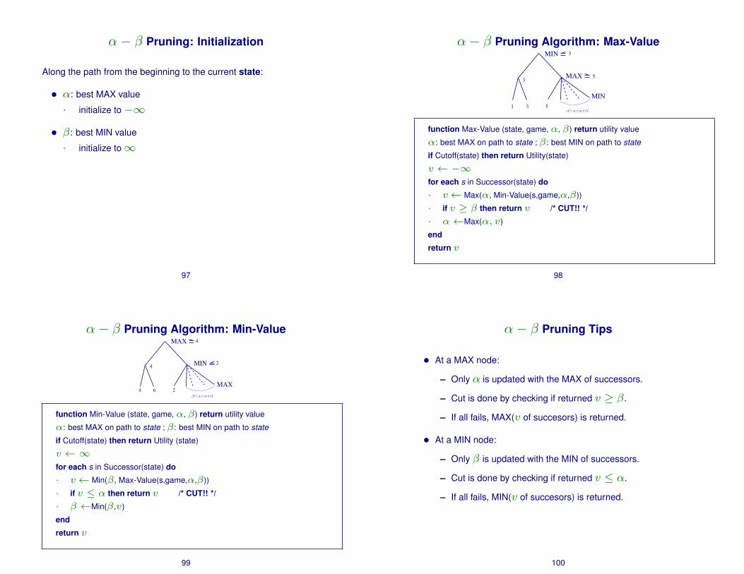
α− β Pruning Algorithm: Min-Value

4 6 2

4

MAX

MIN

MAX

2

4

discard

function Min-Value (state, game, α, β) return utility value

α: best MAX on path to state ; β: best MIN on path to state

if Cutoff(state) then return Utility (state)

v ←∞for each s in Successor(state) do

· v← Min(β, Max-Value(s,game,α,β))

· if v ≤ α then return v /* CUT!! */

· β ←Min(β,v)

end

return v

99

α− β Pruning Tips

• At a MAX node:

– Only α is updated with the MAX of successors.

– Cut is done by checking if returned v ≥ β.

– If all fails, MAX(v of succesors) is returned.

• At a MIN node:

– Only β is updated with the MIN of successors.

– Cut is done by checking if returned v ≤ α.

– If all fails, MIN(v of succesors) is returned.

100

Ordering is Important for Good Pruning

4 6 2

4

MAX

MIN

MAX

2

4

discard4 6

4

MAX

MIN

MAX

2

4

discard5 10 2

• For MIN, sorting successor’s utility in an increasing order is

better (shown above; left).

• For MAX, sorting in decreasing order is better.

101

Games With an Element of Chance

Rolling the dice, shuffling the deck of card and drawing, etc.

• chance nodes need to be included in the minimax tree

• try to make a move that maximizes the expected value→expectimax

• expected value of random variableX :

E(X) =∑

x

xP (x)

• expectimax

expectimax(C) =∑

i

P (di)maxs∈S(C,di)(utility(s))

102

Game Tree With Chance Element

MAX

dice

MIN

dice

MAX• chance element forms a new ply (e.g. dice, shown above)

103

Design Considerations for Probabilistic Games

• the value of evaluation function, not just the scale matters now!

(think of what expected value is)

• time complexity: bmnm, where n is the number of distinct dice

rolls

• pruning can be done if we are careful

104

State of the Art in Gaming With AI

• Chess: IBM’s Deep Blue defeated Garry Kasparov (1997)

• Backgammon: Tesauro’s Neural Network→ top three (1992)

• Othello: smaller search space→ superhuman performance

• Checkers: Samuel’s Checker Program running on 10Kbyte (1952)

Genetic algorithms can perform very well on select domains.

105

Hard Games

The game of Go, popular in East Asia:

• 19× 19 = 361 grid: branching factor is huge!

• brute-force search methods inevitably fail: need more structured

rules

• the bet was high: $1,400,000 prize for the first computer program

to beat a select, 12-year old player. The late Mr. Ing Chang Ki

(photo above) put up the money from his personal funds.

Photo from http://www.samsloan.com/ing.htm.

106

Google DeepMind’s AlphaGo

• AlphaGo by Google DeepMind beat the Korean Go grand master Lee

Sedol in 2015 (4 to 1).

• AlphaGo combined deep reinforcement learning with tree search.

107

Key Points

• formal α− β pruning algorithm: know how to apply pruning

• α− β pruning properties: evaluation

• games with an element of chance: what are the added elements?

how does the minmax tree get augmented?

108