screening and response surface: conceptschamilo2.grenet.fr/inp/courses/ense3m2semaaaa0/... ·...
TRANSCRIPT

21/01/2014 • 1
Screening and Response surface: Concepts
Jean-Louis COULOMB
UMR CNRS 5269 - Grenoble-INP
– Université Joseph Fourier
January 2014
Screening - Response Surface

21/01/2014 Screening - Response Surface • 2
1. Introduction: Direct optimization
Direct optimization
Optimization algorithm controls the objective function directly.
Cost optimization depends linearly on the number of tests and their unit cost.
When the unit cost is important (long simulation or prototype building), there is a need to control the overall cost optimization.
Response Surface and Screening (parts of Design Of Experiments) address this need.
Optimization
algorithm
Objective
function
x
f(x)

21/01/2014 Screening - Response Surface • 3
1. Introduction: Indirect optimization
Indirect optimization
Optimization algorithm is applied to an approximation of the objective function.
This approximation is called Response Surface.
The response surface can be constructed a priori (before optimization) or during the optimization process (then it can be adaptive).
The cost of the calls to the approximation is negligible. Only the number of evaluations of the objective function account.
Optimization
algorithm
Response
surface
x
f ap (x)
Objective
function
x grid
f( x grid )
Numerous
inexpensive
calls
Few
expensive
calls

21/01/2014 Screening - Response Surface • 4
1. Introduction: Screening
Screening
The screening is based on a simple response surface (polynomials of order 1 or 2).
The coefficients of variables and interactions are identified by means of a minimum number of tests
The most important coefficients are the mark of the most significant variables and interactions.
Not significant variables can be fixed which significantly reduces the optimization cost.
Screening
x 1 , x 2 , x 3 , … x 1 x 2 , x 2 x 3 , …
Direct
optimization
Indirect
optimization
x 1 , x 3

21/01/2014 Screening - Response Surface • 5
Summary
1. Introduction
2. Design Of Experiments
3. Response Surface
4. Design Of Experiments Practical work – Role playing

21/01/2014 Screening - Response Surface • 6
2. Design Of Experiments: History
1925: Agricultural research (Fisher) An area where experiments are long, expensive and the results are subject to variability.
It was a method to get from a given number of trials, a maximum credible information on the influence of factors and their prioritization.
1945-1960: Enrichment by statisticians (Box, Hunter) They introduced fractional plans at two levels, central composite designs and associated response surface models.
1960: Quality Approach (Taguchi) Build quality upstream from the design.
Design efficient products on average with small variation around this average.
Made efficiency less sensitive to conditions of use, to manufacturing variations and aging (robust design).

21/01/2014 Screening - Response Surface • 7
2. Design Of Experiments: Surface response: Example
Find a Surface Response for reaction efficiency Y as a function of three factors each with two levels
The study is conducted sequentially in three stages to minimize the number of experiments:
Step 1: Estimate the variability of the response Y.
Step 2: Postulate for Y a linear model without interaction.
Step 3 (if step 2 fails): Postulate for Y a linear model with interactions.
Factor Meaning Lower level Upper level Normalized - Normalized +
X1 Temperature (℃) 100 200 x1= 1 x1= +1
X2 Pressure (bar) 1 2 x2= 1 x2= +1
X3 Catalyser Product 1 Product 2 x3= 1 x3= +1

21/01/2014 Screening - Response Surface • 8
2. Design Of Experiments: Example Step 1
Step 1: Estimate the variability of the response Y Typically, this estimation is achieved by repetition of the experiment at the center of the domain. Here, this is impossible because the factor X3 is a discrete factor.
We choose to repeat 3 experiments X1=150℃ X2=1.5 bars X3=Product 2
The 3 answers are Y1=40.3% Y2=39.8% Y3=40.9%
The average is = 40.33%
The standard deviation is = 0.55%
The experimental error is quite low => a DOE is possible
Note: When results come from simulations => there is no variability
3213
1YYYY
2
3
2
2
2
113
1' YYYYYY
21/01/2014 Screening - Response Surface • 9
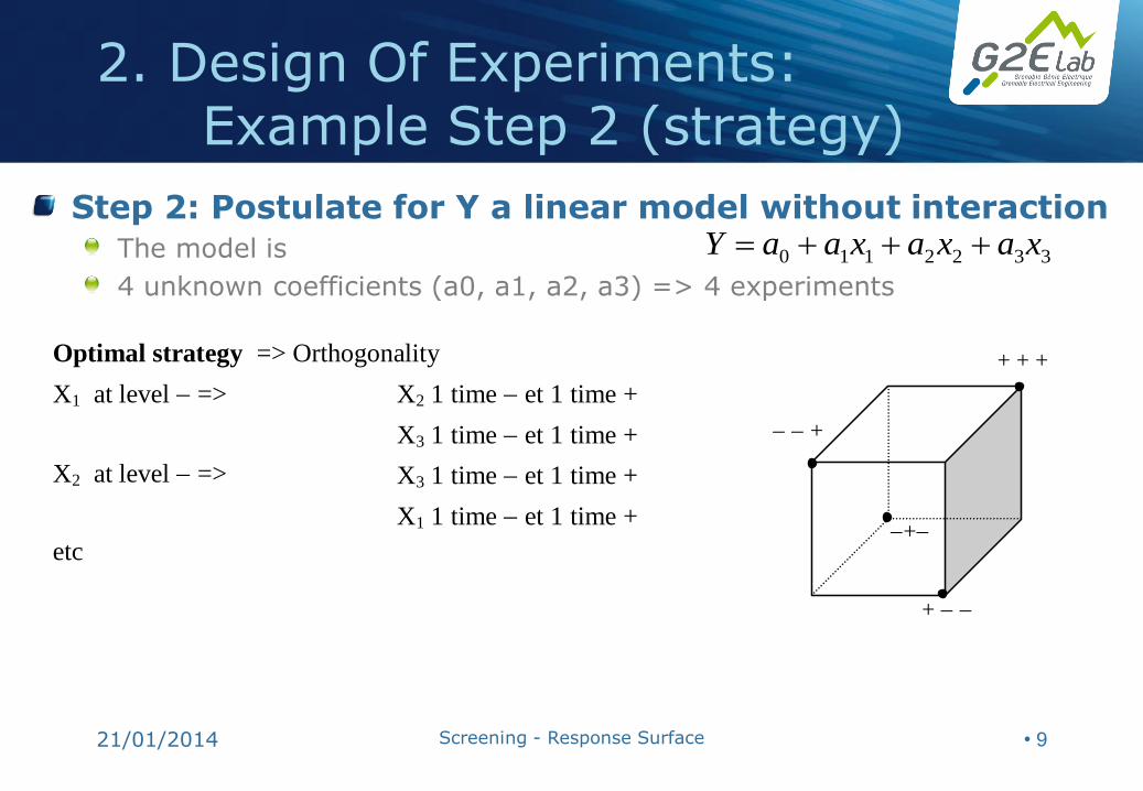
2. Design Of Experiments: Example Step 2 (strategy)
Step 2: Postulate for Y a linear model without interaction The model is
4 unknown coefficients (a0, a1, a2, a3) => 4 experiments
3322110 xaxaxaaY
Optimal strategy => Orthogonality + + +
+
+
+
X1 at level =>
X2 at level =>
etc
X2 1 time et 1 time +
X3 1 time et 1 time +
X3 1 time et 1 time +
X1 1 time et 1 time +
N° experiment Factor X1 (°C) Factor X2 (bar) Factor X3 Response Y (%)
1 200 2 Product 2 75
2 100 2 Product 1 56
3 200 1 Product 1 14
4 100 1 Product 2 9
21/01/2014 Screening - Response Surface • 10
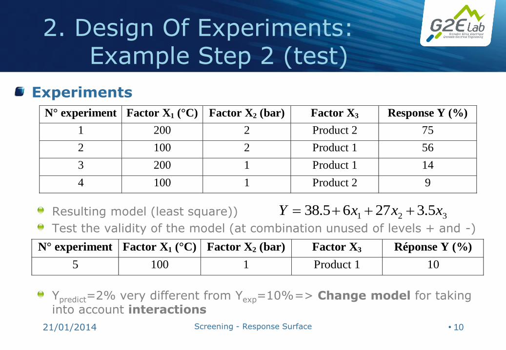
2. Design Of Experiments: Example Step 2 (test)
Experiments
Resulting model (least square))
Test the validity of the model (at combination unused of levels + and -)
Ypredict=2% very different from Yexp=10% => Change model for taking into account interactions
321 5.32765.38 xxxY
N° experiment Factor X1 (°C) Factor X2 (bar) Factor X3 Réponse Y (%)
5 100 1 Product 1 10

21/01/2014 Screening - Response Surface • 11
2. Design Of Experiments: Example Step 3 (strategy)
Step 3: Postulate for Y a linear model with interactions Model
8 unknown coefficients => 8 experiments
Optimal strategy => Full factorial design at 2 levels
5 tests are already available
• 4 for building the previous model
• +1 for testing
Only three additional experiments to perform (sequentiality)!
3211233223311321123322110 xxxaxxaxxaxxaxaxaxaaY
N° experiment Factor X1 (°C) Factor X2 (bar) Factor X3 Response Y (%)
6 200 2 Product 1 66
7 200 1 Product 2 34
8 100 2 Product 2 45

21/01/2014 Screening - Response Surface • 12
2. Design Of Experiments: Example Step 3 (test)
Resulting model
The absolute value of a coefficient given the impact of the linear effect or interaction.
The interaction x1x2x3 is negligible => refined model
Test the validity of the model Central point of start of the study (can ensure absence of non-linearity) X1=150°C, X2=1.5 bars, X3= Product 2 Responses are Y1=40.3% Y2=39.8% Y3=40.9% => Ypredict = 40.73%
Small difference => this linear model with interactions seems acceptable
We ignore here the statistical validation which is an important part of the method for real experiments (not for numerical)
Usable for interpolation only (NOT for extrapolation)
321323121321 13.063.213.538.113.288.2163.863.38 xxxxxxxxxxxxY
323121321 63.213.538.113.288.2163.863.38 xxxxxxxxxY

21/01/2014 Screening - Response Surface • 13
2. Design Of Experiments: Methodology in brief
Define N factors and the experimental region of interest
Define the normalized variables associated with variable factors
Step 1: Apply a non-linear interaction model
Conduct experiments
Determine the linear model without interaction
Validate the model
Exploitation of the linear model without interaction
Step 2 (if previous model not valid): Apply a linear model with interactions
Conduct experiments
Determine the linear model with interactions
Validate the model (center field)
Exploitation of the linear model with interaction
Step 3 (if previous model not valid): Apply a second degree model ...

21/01/2014 Screening - Response Surface • 14
2. Design Of Experiments: Fractional factorial designs
Now we have more factors, but hopefully we know a “good” model
We know that the model depends on 4 factors and only 3 of first order interactions
If we implement a 24 factorial design, it will take 16 experiences while 8 would be sufficient!
Idea
Take a subset of the 24 factorial design that respects the orthogonality between factors.
There are tables that provide designs based on the number of factors and the number of experiments (power of 2) desired (Box, Hunter and Hunter).
Note
We do not calculate the effects (a1, a13, ...) but additions of effects (a1+a234, a13+a24, ...) called contrasts (we say that a1 is an alias for a234 ...).
This introduces confusions that depend on the DOE and on the order of the factors in this DOE.
Using known a priori information on significant interactions (a234=a24= ... =0), the experimenter can choose a design such that the remaining effects (a1, a13, ...) are calculated.
433432233113443322110 xxaxxaxxaxaxaxaxaaY

21/01/2014 Screening - Response Surface • 15
2. Design Of Experiments: Summary
Design of experiments for the experimenter are a very effective way
To determine the influential factors of a system (screening)
To predict the response of a system (response surface)
Optimize system (at least second degree response surface)
The analysis of the variability of response (not shown in the introduction) allows
To build quality upstream from the design
Design efficient products on average with small variation around this average
To make the efficiency less sensitive to conditions of use, to manufacturing variations and aging (robust design)
For the numerical DOE we retain The method of screening before optimization to eliminate non-influential factors
The response surface method in place of direct calculation of the objective function

21/01/2014 Screening - Response Surface • 16
3. Response Surface: Classical Response Surfaces
Classical Response Surfaces (1st and 2nd order polynomial) Polynomial of degree 1 without interaction
Polynomial of degree 1 with interactions
Polynomial of degree 2
normalized variables,
the center value, and coefficients of the main effects and the coefficients of interactions.
These unknown coefficients can be determined by the least squares method
At least as many experiments of the objective function as unknown coefficients
Some additional experiments allow to test the response surface
Allow screening absolute value of a coefficient = impact of an effect
n
i
ii xaaxf1
0)(
1
1 11
0)(n
i
n
ij
jiij
n
i
ii xxaxaaxf
n
i
iii
n
i
n
ij
jiij
n
i
ii xaxxaxaaxf1
21
1 11
0)(
ix
0a ia iiaija

21/01/2014 Screening - Response Surface • 17
3. Response Surface: 1st order without interaction
Which experiments to choose? Fractional factorial designs at two levels
Nb
variables
Response Surface Nb
coefficients
1 110)( xaaxf 2
2 222110)( xaxaaxf 3
3 3322110)( xaxaxaaxf 4
… … …
n
n
iii xaaxf
10)(
1+n

21/01/2014 Screening - Response Surface • 18
3. Response Surface: 1st order with first interactions
Which experiments to choose? Fractional factorial designs at two levels
Nb
variables
Response Surface Nb
coefficients
1 110)( xaaxf 2
2 211222110)( xxaxaxaaxf 4
3 3113322321123322110)( xxaxxaxxaxaxaxaaxf 7
… … …
n
1
1 110)(
n
i
n
ijjiij
n
iii xxaxaaxf
2
)1.(1
nn
21/01/2014 Screening - Response Surface • 19
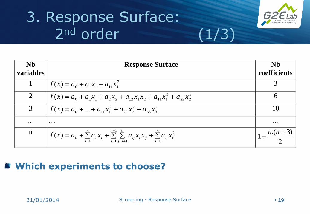
3. Response Surface: 2nd order (1/3)
Which experiments to choose?
Nb
variables
Response Surface Nb
coefficients
1 2
111110)( xaxaaxf 3
2 2
222
2
111211222110)( xaxaxxaxaxaaxf 6
3 2
3133
2
222
2
1110 ...)( xaxaxaaxf 10
… … …
n
n
iiii
n
i
n
ijjiij
n
iii xaxxaxaaxf
1
21
1 110)(
2
)3.(1
nn
21/01/2014 Screening - Response Surface • 20
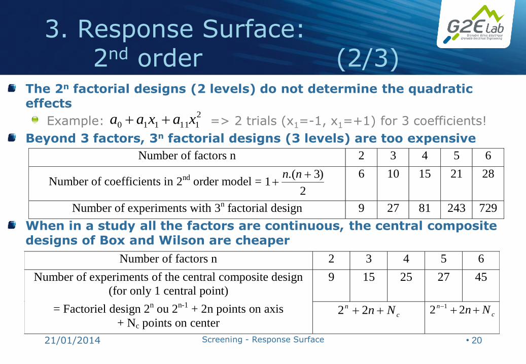
3. Response Surface: 2nd order (2/3)
The 2n factorial designs (2 levels) do not determine the quadratic effects
Example: => 2 trials (x1=-1, x1=+1) for 3 coefficients!
Beyond 3 factors, 3n factorial designs (3 levels) are too expensive
When in a study all the factors are continuous, the central composite designs of Box and Wilson are cheaper
2
111110 xaxaa
Number of factors n 2 3 4 5 6
Number of coefficients in 2nd order model = 2
)3.(1
nn
6 10 15 21 28
Number of experiments with 3n factorial design 9 27 81 243 729
Number of factors n 2 3 4 5 6
Number of experiments of the central composite design
(for only 1 central point)
9 15 25 27 45
= Factoriel design 2n ou 2n-1 + 2n points on axis
+ Nc points on center c
n Nn 22 c
n Nn 22 1

21/01/2014 Screening - Response Surface • 21
3. Response Surface: 2nd order (3/3)
Spherical central composite design
5 levels (, 1, 0, +1, +)
For n=3 : =1.682 and Nc=6
Tradeoff between
=> quasi-orthogonality
=> isovariance by rotation
=> uniform accuracy
Cubical central composite design
Only 3 levels (1, 0, +1)
Simpler

21/01/2014 Screening - Response Surface • 22
3. Response Surface: Classical Response Surfaces
Advantages and drawbacks of classical response surfaces
Advantages :
They allow the examination of the main
effects of factors and their interactions.
This can be used to exclude the least
significant factors before optimization
(screening).
Function with three local minima and a global
minimum
Drawbacks :
These response surfaces cannot replace a
multimodal function (with multiple optima).

21/01/2014 Screening - Response Surface • 23
3. Response Surface: Generalised Response Surfaces
Aim Provide a correct approximation method for multimodal function
Principles common to generalized response surface Grid points M (possibly refined around the optimum)
Approximation of the form
Method of radial basis functions Inverse multiquadric
Gaussian
M
j
jj xxhcxf1
2jxx
j exxh

21/01/2014 Screening - Response Surface • 24
4. Design Of experiments: Pratical work
Experiment “Design Of Experiments” Document “Role playing”