methods for analysis and control of dynamical systems...

Control ofdynamical systems

O.Sename

Introduction

Concept

Rules

DynamiccompensationSpecifications

Case of PID controllers

Lead compensation

Lag compensation

Matlab examples

Methods for analysis and control of dynamical systemsLecture 4: The root locus design method

O. Sename1

1Gipsa-lab, CNRS-INPG, [email protected]

www.gipsa-lab.fr/∼o.sename

5th February 2015


O.Sename

Introduction

Concept

Rules



Lead compensation

Lag compensation

Matlab examples

Outline

Introduction

Concept

Rules

Dynamic compensationSpecificationsCase of PID controllersLead compensationLag compensation

Matlab examples


O.Sename

Introduction

Concept

Rules



Lead compensation

Lag compensation

Matlab examples

References

Some interesting books:I G. Franklin, J. Powell, A. Emami-Naeini, Feedback Control of

Dynamic Systems, Prentice Hall, 2005I R.C. Dorf and R.H. Bishop, Modern Control Systems, Prentice

Hall, USA, 2005.I P.Borne, G.Dauphin-Tanguy, J.P.Richard, F.Rotella, I.Zambettakis,

Analyse et Régulation des processus industriels. Tome 1:Régulation continue, Méthodes et pratiques de l’ingénieur, EditionsTechnip, 1993.


O.Sename

Introduction

Concept

Rules



Lead compensation

Lag compensation

Matlab examples

Definition

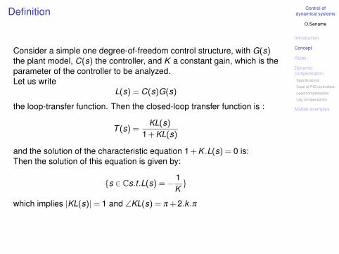
Consider a simple one degree-of-freedom control structure, with G(s)the plant model, C(s) the controller, and K a constant gain, which is theparameter of the controller to be analyzed.Let us write

L(s) = C(s)G(s)

the loop-transfer function. Then the closed-loop transfer function is :

T (s) =KL(s)

1+KL(s)

and the solution of the characteristic equation 1+K .L(s) = 0 is:Then the solution of this equation is given by:

{s ∈ Cs.t .L(s) =− 1K}

which implies |KL(s)|= 1 and ∠KL(s) = π +2.k .π


O.Sename

Introduction

Concept

Rules



Lead compensation

Lag compensation

Matlab examples

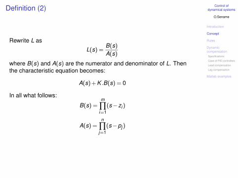
Definition (2)

Rewrite L as

L(s) =B(s)A(s)

where B(s) and A(s) are the numerator and denominator of L. Thenthe characteristic equation becomes:

A(s)+K .B(s) = 0

In all what follows:

B(s) =m

∏i=1

(s−zi )

A(s) =n

∏j=1

(s−pj )


O.Sename

Introduction

Concept

Rules



Lead compensation

Lag compensation

Matlab examples

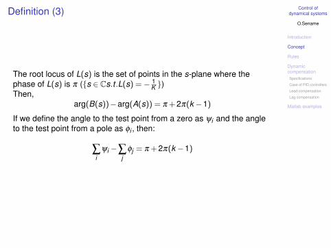
Definition (3)

The root locus of L(s) is the set of points in the s-plane where thephase of L(s) is π ({s ∈ Cs.t .L(s) =− 1

K })Then,

arg(B(s))−arg(A(s)) = π +2π(k −1)

If we define the angle to the test point from a zero as ψi and the angleto the test point from a pole as φi , then:

∑i

ψi −∑j

φj = π +2π(k −1)


O.Sename

Introduction

Concept

Rules



Lead compensation

Lag compensation

Matlab examples

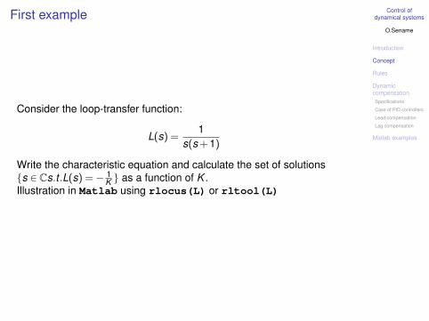
First example

Consider the loop-transfer function:

L(s) =1

s(s+1)

Write the characteristic equation and calculate the set of solutions{s ∈ Cs.t .L(s) =− 1

K } as a function of K .Illustration in Matlab using rlocus(L) or rltool(L)


O.Sename

Introduction

Concept

Rules



Lead compensation

Lag compensation

Matlab examples

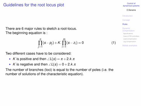
Guidelines for the root locus plot

There are 6 major rules to sketch a root-locus.The beginning equation is :

n

∏j=1

(s−pj )+K .m

∏i=1

(s−zi ) = 0 (1)

Two different cases have to be considered:I K is positive and then ∠L(s) = π +2.k .πI K is negative and then ∠L(s) = 0+2.k .π

The number of branches (loci) is equal to the number of poles (i.e. thenumber of solutions of the characteristic equation).


O.Sename

Introduction

Concept

Rules



Lead compensation

Lag compensation

Matlab examples

Rule 1: departure and arrival

Rule 1The n branches of the locus start at the poles of L(s) and m of thesebranches end on the zeros of L(s)

Indeed:

1. When K = 0, the solution of equation (1) are the poles pj .

2. from L(s) =− 1K , as K → ∞, the equation reduces to L(s) = 0, i.e.

B(s) = 0 which corresponds to the zeros of L

Example :

L(s) =1

s(s2 +8s+32)


O.Sename

Introduction

Concept

Rules



Lead compensation

Lag compensation

Matlab examples

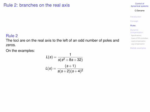
Rule 2: branches on the real axis

Rule 2The loci are on the real axis to the left of an odd number of poles andzeros.

On the examples:

L(s) =1

s(s2 +8s+32)

L(s) =(s+1)

s(s+2)(s+4)2


O.Sename

Introduction

Concept

Rules



Lead compensation

Lag compensation

Matlab examples

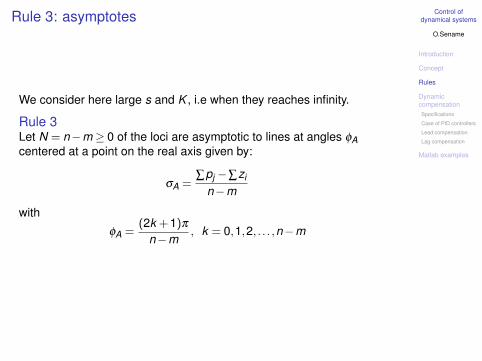
Rule 3: asymptotes

We consider here large s and K , i.e when they reaches infinity.

Rule 3Let N = n−m ≥ 0 of the loci are asymptotic to lines at angles φAcentered at a point on the real axis given by:

σA =∑pj −∑zi

n−m

with

φA =(2k +1)π

n−m, k = 0,1,2, . . . ,n−m


O.Sename

Introduction

Concept

Rules



Lead compensation

Lag compensation

Matlab examples

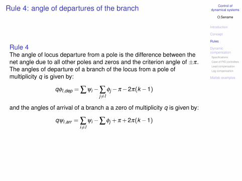
Rule 4: angle of departures of the branch

Rule 4The angle of locus departure from a pole is the difference between thenet angle due to all other poles and zeros and the criterion angle of ±π.The angles of departure of a branch of the locus from a pole ofmultiplicity q is given by:

qφl ,dep = ∑ψi −∑j 6=l

φj −π−2π(k −1)

and the angles of arrival of a branch a a zero of multiplicity q is given by:

qψl ,arr = ∑i 6=l

ψi −∑φj +π +2π(k −1)


O.Sename

Introduction

Concept

Rules



Lead compensation

Lag compensation

Matlab examples

Rule 5

Rule 5The root locus crosses the jω axis at points where the Routh criterionshows a transition from roots in the left-plane to roots in the right halfplane.

Example: L(s) = 1s(s2+8s+32) .

Rouths3 1 32s2 8 Ks1 8×32−K

8 0s0 K

For K = 0, there is a root at s = 0.No RHP roots for 0 < K < 8×32 = 256.When K = 256 roots on the jω axis (ωc = 5.66).


O.Sename

Introduction

Concept

Rules



Lead compensation

Lag compensation

Matlab examples

Rule 6: breakaway point

Rule 6The equation to be solved can be rewritten as:

A(s)B(s)

=−K

which means that the set of solutions changes of direction (tangents)whenever d

ds (A(s)B(s) ) = 0

The locus will have multiple roots at points on the locus where thederivative is zero, or:

BdAds−A

dBds

= 0


O.Sename

Introduction

Concept

Rules



Lead compensation

Lag compensation

Matlab examples

Root locus for satellite attitude control with PD control

The characteristic equation is :

1+[kp +kd s]1s2 = 0

Assume kp/kd = α is known, and note K = kd . Then it leads

1+Ks+α

s2 = 0

I R1: There are 2 branches that start at s = 0 and 1 which ends ats =−α

I R2: The real axis to the left of s =−α is on the locusI R3: There is one asymptote (n-m=1) at σA = α of angle φA = π


O.Sename

Introduction

Concept

Rules



Lead compensation

Lag compensation

Matlab examples

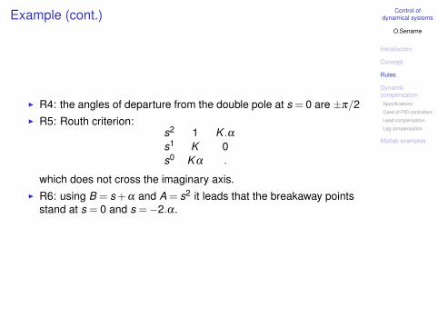
Example (cont.)

I R4: the angles of departure from the double pole at s = 0 are ±π/2I R5: Routh criterion:

s2 1 K .α

s1 K 0s0 K α .

which does not cross the imaginary axis.I R6: using B = s+α and A = s2 it leads that the breakaway points

stand at s = 0 and s =−2.α.


O.Sename

Introduction

Concept

Rules



Lead compensation

Lag compensation

Matlab examples

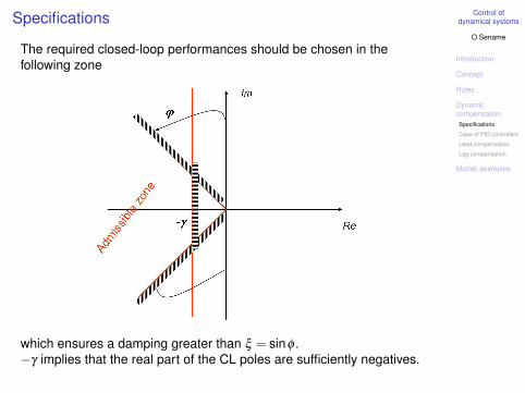
Specifications

The required closed-loop performances should be chosen in thefollowing zone

which ensures a damping greater than ξ = sinφ .−γ implies that the real part of the CL poles are sufficiently negatives.


O.Sename

Introduction

Concept

Rules



Lead compensation

Lag compensation

Matlab examples

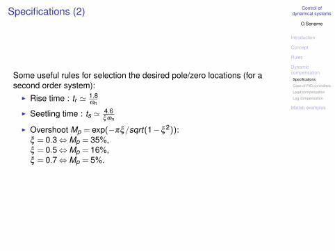
Specifications (2)

Some useful rules for selection the desired pole/zero locations (for asecond order system):

I Rise time : tr ' 1.8ωn

I Seetling time : ts ' 4.6ξ ωn

I Overshoot Mp = exp(−πξ/sqrt(1−ξ 2)):ξ = 0.3⇔Mp = 35%,ξ = 0.5⇔Mp = 16%,ξ = 0.7⇔Mp = 5%.


O.Sename

Introduction

Concept

Rules



Lead compensation

Lag compensation

Matlab examples

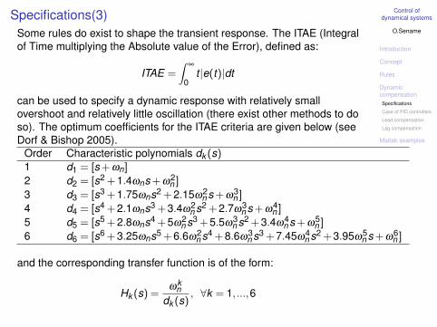
Specifications(3)Some rules do exist to shape the transient response. The ITAE (Integralof Time multiplying the Absolute value of the Error), defined as:

ITAE =∫

∞

0t |e(t)|dt

can be used to specify a dynamic response with relatively smallovershoot and relatively little oscillation (there exist other methods to doso). The optimum coefficients for the ITAE criteria are given below (seeDorf & Bishop 2005).

Order Characteristic polynomials dk (s)1 d1 = [s+ωn]

2 d2 = [s2 +1.4ωns+ω2n ]

3 d3 = [s3 +1.75ωns2 +2.15ω2n s+ω3

n ]

4 d4 = [s4 +2.1ωns3 +3.4ω2n s2 +2.7ω3

n s+ω4n ]

5 d5 = [s5 +2.8ωns4 +5ω2n s3 +5.5ω3

n s2 +3.4ω4n s+ω5

n ]

6 d6 = [s6 +3.25ωns5 +6.6ω2n s4 +8.6ω3

n s3 +7.45ω4n s2 +3.95ω5

n s+ω6n ]

and the corresponding transfer function is of the form:

Hk (s) =ωk

ndk (s)

, ∀k = 1, ...,6


O.Sename

Introduction

Concept

Rules



Lead compensation

Lag compensation

Matlab examples

Specifications(4)

0 2 4 6 8 10 12 14 160

0.2

0.4

0.6

0.8

1

1.2

NORMALIZED TIME ωn t

H1H2H3H4H5H6

STEP RESPONSE OF TRANSFER FUNCTIONSWITH ITAE CHARACTERISTIC POLYNOMIALS


O.Sename

Introduction

Concept

Rules



Lead compensation

Lag compensation

Matlab examples

PID controller

A PID controller is given by:

C(s) = Kp(1+1

Ti s+Td s) = Kp +KD s+

KIs

For convenience it will be rewritten as :

C(s) = KD(s+z1)(s+z2)

s

which has one pole at the origine and two stable zeros.


O.Sename

Introduction

Concept

Rules



Lead compensation

Lag compensation

Matlab examples

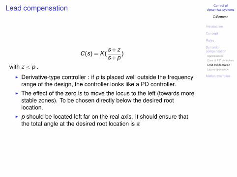
Lead compensation

C(s) = K (s+zs+p

)

with z < p .

I Derivative-type controller : if p is placed well outside the frequencyrange of the design, the controller looks like a PD controller.

I The effect of the zero is to move the locus to the left (towards morestable zones). To be chosen directly below the desired rootlocation.

I p should be located left far on the real axis. It should ensure thatthe total angle at the desired root location is π


O.Sename

Introduction

Concept

Rules



Lead compensation

Lag compensation

Matlab examples

Lag compensation

C(s) = K (s+zs+p

)

with z > p.I Integration-type controller:I p should be closed to the origine. z sufficiently far.I z/p is chosen to be between 3 and 10 (according to the need of

boosting the steady-state gain).


O.Sename

Introduction

Concept

Rules



Lead compensation

Lag compensation

Matlab examples

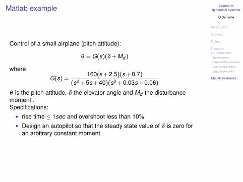
Matlab example

Control of a small airplane (pitch attitude):

θ = G(s)(δ +Md )

where

G(s) =160(s+2.5)(s+0.7)

(s2 +5s+40)(s2 +0.03s+0.06)

θ is the pitch attitude, δ the elevator angle and Md the disturbancemoment .Specifications:

I rise time ≤ 1sec and overshoot less than 10%I Design an autopilot so that the steady state value of δ is zero for

an arbitrary constant moment.


O.Sename

Introduction

Concept

Rules



Lead compensation

Lag compensation

Matlab examples

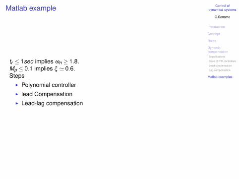
Matlab example

tr ≤ 1sec implies ωn ≥ 1.8.Mp ≤ 0.1 implies ξ ' 0.6.Steps

I Polynomial controllerI lead CompensationI Lead-lag compensation

methods for analysis and control of dynamical systems...

Documents