scientiﬁc computing: an introductory surveyheath.cs.illinois.edu/scicomp/notes/chap02.pdf ·...

Existence, Uniqueness, and ConditioningSolving Linear Systems

Special Types of Linear SystemsSoftware for Linear Systems

Scientific Computing: An Introductory SurveyChapter 2 – Systems of Linear Equations

Prof. Michael T. Heath

Department of Computer ScienceUniversity of Illinois at Urbana-Champaign

Copyright c© 2002. Reproduction permittedfor noncommercial, educational use only.

Michael T. Heath Scientific Computing 1 / 88



Outline

1 Existence, Uniqueness, and Conditioning

2 Solving Linear Systems

3 Special Types of Linear Systems

4 Software for Linear Systems




Singularity and NonsingularityNormsCondition NumberError Bounds

Systems of Linear Equations

Given m× n matrix A and m-vector b, find unknownn-vector x satisfying Ax = b

System of equations asks “Can b be expressed as linearcombination of columns of A?”

If so, coefficients of linear combination are given bycomponents of solution vector x

Solution may or may not exist, and may or may not beunique

For now, we consider only square case, m = n





Singularity and Nonsingularity

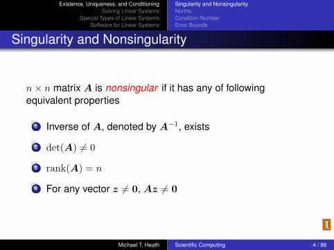
n× n matrix A is nonsingular if it has any of followingequivalent properties

1 Inverse of A, denoted by A−1, exists

2 det(A) 6= 0

3 rank(A) = n

4 For any vector z 6= 0, Az 6= 0





Existence and Uniqueness

Existence and uniqueness of solution to Ax = b dependon whether A is singular or nonsingular

Can also depend on b, but only in singular case

If b ∈ span(A), system is consistent

A b # solutionsnonsingular arbitrary one (unique)

singular b ∈ span(A) infinitely manysingular b /∈ span(A) none





Geometric Interpretation

In two dimensions, each equation determines straight linein plane

Solution is intersection point of two lines

If two straight lines are not parallel (nonsingular), thenintersection point is unique

If two straight lines are parallel (singular), then lines eitherdo not intersect (no solution) or else coincide (any pointalong line is solution)

In higher dimensions, each equation determineshyperplane; if matrix is nonsingular, intersection ofhyperplanes is unique solution





Example: Nonsingularity

2× 2 system

2x1 + 3x2 = b1

5x1 + 4x2 = b2

or in matrix-vector notation

Ax =

[2 35 4

] [x1x2

]=

[b1b2

]= b

is nonsingular regardless of value of b

For example, if b =[8 13

]T , then x =[1 2

]T is uniquesolution





Example: Singularity

2× 2 system

Ax =

[2 34 6

] [x1x2

]=

[b1b2

]= b

is singular regardless of value of b

With b =[4 7

]T , there is no solution

With b =[4 8

]T , x =[γ (4− 2γ)/3

]T is solution for anyreal number γ, so there are infinitely many solutions





Vector Norms

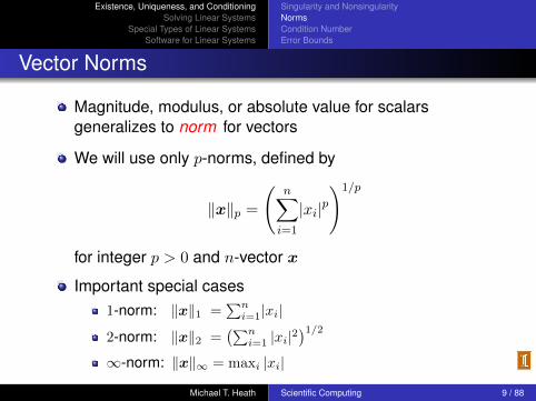
Magnitude, modulus, or absolute value for scalarsgeneralizes to norm for vectors

We will use only p-norms, defined by

‖x‖p =

(n∑

i=1

|xi|p)1/p

for integer p > 0 and n-vector x

Important special cases1-norm: ‖x‖1 =

∑ni=1|xi|

2-norm: ‖x‖2 =(∑n

i=1 |xi|2)1/2

∞-norm: ‖x‖∞ = maxi |xi|





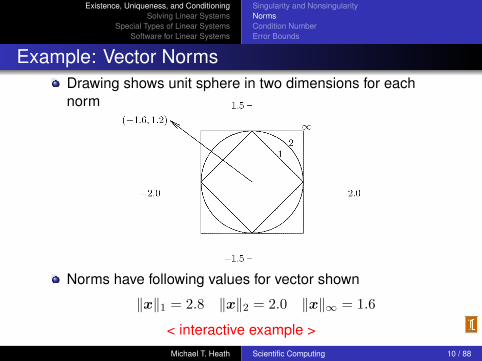
Example: Vector NormsDrawing shows unit sphere in two dimensions for eachnorm

Norms have following values for vector shown

‖x‖1 = 2.8 ‖x‖2 = 2.0 ‖x‖∞ = 1.6

< interactive example >Michael T. Heath Scientific Computing 10 / 88

http://www.cs.illinois.edu/~heath/iem/linear_equations/pnorms/




Equivalence of Norms

In general, for any vector x in Rn, ‖x‖1 ≥ ‖x‖2 ≥ ‖x‖∞

However, we also have

‖x‖1 ≤√n ‖x‖2, ‖x‖2 ≤

√n ‖x‖∞, ‖x‖1 ≤ n ‖x‖∞

Thus, for given n, norms differ by at most a constant, andhence are equivalent: if one is small, they must all beproportionally small.





Properties of Vector Norms

For any vector norm

‖x‖ > 0 if x 6= 0

‖γx‖ = |γ| · ‖x‖ for any scalar γ‖x + y‖ ≤ ‖x‖+ ‖y‖ (triangle inequality)

In more general treatment, these properties taken asdefinition of vector norm

Useful variation on triangle inequality

| ‖x‖ − ‖y‖ | ≤ ‖x− y‖





Matrix Norms

Matrix norm corresponding to given vector norm is definedby

‖A‖ = maxx6=0‖Ax‖‖x‖

Norm of matrix measures maximum stretching matrix doesto any vector in given vector norm





Matrix Norms

Matrix norm corresponding to vector 1-norm is maximumabsolute column sum

‖A‖1 = maxj

n∑i=1

|aij |

Matrix norm corresponding to vector∞-norm is maximumabsolute row sum

‖A‖∞ = maxi

n∑j=1

|aij |

Handy way to remember these is that matrix norms agreewith corresponding vector norms for n× 1 matrix





Properties of Matrix Norms

Any matrix norm satisfies

‖A‖ > 0 if A 6= 0

‖γA‖ = |γ| · ‖A‖ for any scalar γ‖A + B‖ ≤ ‖A‖+ ‖B‖

Matrix norms we have defined also satisfy

‖AB‖ ≤ ‖A‖ · ‖B‖‖Ax‖ ≤ ‖A‖ · ‖x‖ for any vector x





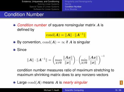
Condition Number

Condition number of square nonsingular matrix A isdefined by

cond(A) = ‖A‖ · ‖A−1‖

By convention, cond(A) =∞ if A is singular

Since

‖A‖ · ‖A−1‖ =

(maxx6=0

‖Ax‖‖x‖

)·(

minx6=0

‖Ax‖‖x‖

)−1condition number measures ratio of maximum stretching tomaximum shrinking matrix does to any nonzero vectors

Large cond(A) means A is nearly singular





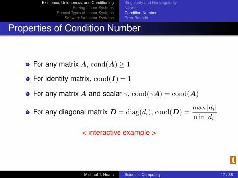
Properties of Condition Number

For any matrix A, cond(A) ≥ 1

For identity matrix, cond(I) = 1

For any matrix A and scalar γ, cond(γA) = cond(A)

For any diagonal matrix D = diag(di), cond(D) =max |di|min |di|

< interactive example >


http://www.cs.illinois.edu/~heath/iem/linear_equations/condition_number/




Computing Condition Number

Definition of condition number involves matrix inverse, so itis nontrivial to compute

Computing condition number from definition would requiremuch more work than computing solution whose accuracyis to be assessed

In practice, condition number is estimated inexpensively asbyproduct of solution process

Matrix norm ‖A‖ is easily computed as maximum absolutecolumn sum (or row sum, depending on norm used)

Estimating ‖A−1‖ at low cost is more challenging





Computing Condition Number, continued

From properties of norms, if Az = y, then

‖z‖‖y‖

≤ ‖A−1‖

and bound is achieved for optimally chosen y

Efficient condition estimators heuristically pick y with largeratio ‖z‖/‖y‖, yielding good estimate for ‖A−1‖

Good software packages for linear systems provideefficient and reliable condition estimator





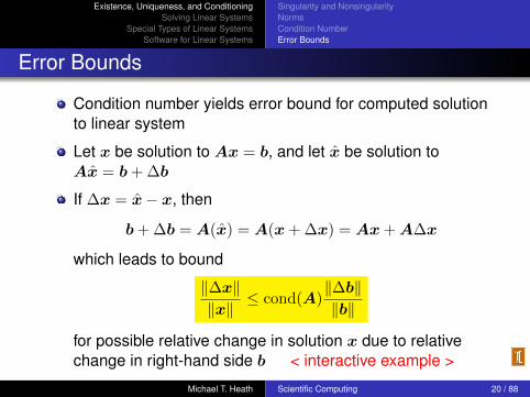
Error Bounds

Condition number yields error bound for computed solutionto linear system

Let x be solution to Ax = b, and let x be solution toAx = b + ∆b

If ∆x = x− x, then

b + ∆b = A(x) = A(x + ∆x) = Ax + A∆x

which leads to bound

‖∆x‖‖x‖

≤ cond(A)‖∆b‖‖b‖

for possible relative change in solution x due to relativechange in right-hand side b < interactive example >


http://www.cs.illinois.edu/~heath/iem/linear_equations/error_bound/




Error Bounds, continued

Similar result holds for relative change in matrix: if(A + E)x = b, then

‖∆x‖‖x‖

≤ cond(A)‖E‖‖A‖

If input data are accurate to machine precision, then boundfor relative error in solution x becomes

‖x− x‖‖x‖

≤ cond(A) εmach

Computed solution loses about log10(cond(A)) decimaldigits of accuracy relative to accuracy of input





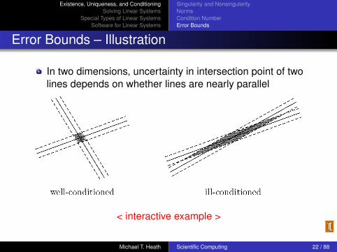
Error Bounds – Illustration

In two dimensions, uncertainty in intersection point of twolines depends on whether lines are nearly parallel



http://www.cs.illinois.edu/~heath/iem/linear_equations/conditioning/




Error Bounds – Caveats

Normwise analysis bounds relative error in largestcomponents of solution; relative error in smallercomponents can be much larger

Componentwise error bounds can be obtained, butsomewhat more complicated

Conditioning of system is affected by relative scaling ofrows or columns

Ill-conditioning can result from poor scaling as well as nearsingularityRescaling can help the former, but not the latter





Residual

Residual vector of approximate solution x to linear systemAx = b is defined by

r = b−Ax

In theory, if A is nonsingular, then ‖x− x‖ = 0 if, and onlyif, ‖r‖ = 0, but they are not necessarily smallsimultaneously

Since‖∆x‖‖x‖

≤ cond(A)‖r‖

‖A‖ · ‖x‖small relative residual implies small relative error inapproximate solution only if A is well-conditioned





Residual, continued

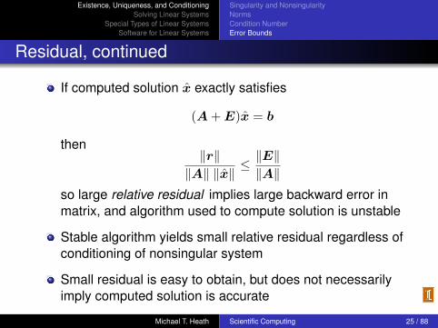
If computed solution x exactly satisfies

(A + E)x = b

then‖r‖

‖A‖ ‖x‖≤ ‖E‖‖A‖

so large relative residual implies large backward error inmatrix, and algorithm used to compute solution is unstable

Stable algorithm yields small relative residual regardless ofconditioning of nonsingular system

Small residual is easy to obtain, but does not necessarilyimply computed solution is accurate




Triangular SystemsGaussian EliminationUpdating SolutionsImproving Accuracy

Solving Linear Systems

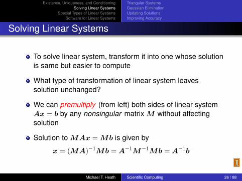
To solve linear system, transform it into one whose solutionis same but easier to compute

What type of transformation of linear system leavessolution unchanged?

We can premultiply (from left) both sides of linear systemAx = b by any nonsingular matrix M without affectingsolution

Solution to MAx = Mb is given by

x = (MA)−1Mb = A−1M−1Mb = A−1b





Example: Permutations

Permutation matrix P has one 1 in each row and columnand zeros elsewhere, i.e., identity matrix with rows orcolumns permuted

Note that P−1 = P T

Premultiplying both sides of system by permutation matrix,PAx = Pb, reorders rows, but solution x is unchanged

Postmultiplying A by permutation matrix, APx = b,reorders columns, which permutes components of originalsolution

x = (AP )−1b = P−1A−1b = P T (A−1b)





Example: Diagonal Scaling

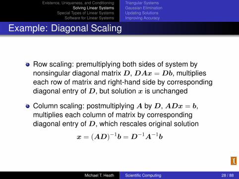
Row scaling: premultiplying both sides of system bynonsingular diagonal matrix D, DAx = Db, multiplieseach row of matrix and right-hand side by correspondingdiagonal entry of D, but solution x is unchanged

Column scaling: postmultiplying A by D, ADx = b,multiplies each column of matrix by correspondingdiagonal entry of D, which rescales original solution

x = (AD)−1b = D−1A−1b





Triangular Linear Systems

What type of linear system is easy to solve?

If one equation in system involves only one component ofsolution (i.e., only one entry in that row of matrix isnonzero), then that component can be computed bydivision

If another equation in system involves only one additionalsolution component, then by substituting one knowncomponent into it, we can solve for other component

If this pattern continues, with only one new solutioncomponent per equation, then all components of solutioncan be computed in succession.

System with this property is called triangular





Triangular Matrices

Two specific triangular forms are of particular interest

lower triangular : all entries above main diagonal are zero,aij = 0 for i < j

upper triangular : all entries below main diagonal are zero,aij = 0 for i > j

Successive substitution process described earlier isespecially easy to formulate for lower or upper triangularsystems

Any triangular matrix can be permuted into upper or lowertriangular form by suitable row permutation





Forward-Substitution

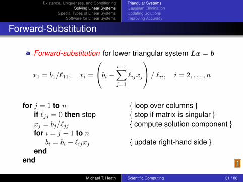
Forward-substitution for lower triangular system Lx = b

x1 = b1/`11, xi =

bi − i−1∑j=1

ìjxj

/ ìi, i = 2, . . . , n

for j = 1 to nif `jj = 0 then stopxj = bj/`jjfor i = j + 1 to n

bi = bi − ìjxjend

end

{ loop over columns }{ stop if matrix is singular }{ compute solution component }

{ update right-hand side }





Back-Substitution

Back-substitution for upper triangular system Ux = b

xn = bn/unn, xi =

bi − n∑j=i+1

uijxj

/ uii, i = n− 1, . . . , 1

for j = n to 1if ujj = 0 then stopxj = bj/ujjfor i = 1 to j − 1

bi = bi − uijxjend

end

{ loop backwards over columns }{ stop if matrix is singular }{ compute solution component }

{ update right-hand side }





Example: Triangular Linear System

2 4 −20 1 10 0 4

x1x2x3

=

248

Using back-substitution for this upper triangular system,last equation, 4x3 = 8, is solved directly to obtain x3 = 2

Next, x3 is substituted into second equation to obtainx2 = 2

Finally, both x3 and x2 are substituted into first equation toobtain x1 = −1





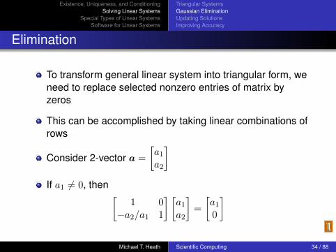
Elimination

To transform general linear system into triangular form, weneed to replace selected nonzero entries of matrix byzeros

This can be accomplished by taking linear combinations ofrows

Consider 2-vector a =

[a1a2

]If a1 6= 0, then [

1 0−a2/a1 1

] [a1a2

]=

[a10

]





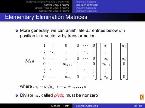
Elementary Elimination Matrices

More generally, we can annihilate all entries below kthposition in n-vector a by transformation

Mka =

1 · · · 0 0 · · · 0...

. . ....

.... . .

...0 · · · 1 0 · · · 00 · · · −mk+1 1 · · · 0...

. . ....

.... . .

...0 · · · −mn 0 · · · 1

a1...akak+1

...an

=

a1...ak0...0

where mi = ai/ak, i = k + 1, . . . , n

Divisor ak, called pivot, must be nonzero





Elementary Elimination Matrices, continued

Matrix Mk, called elementary elimination matrix, addsmultiple of row k to each subsequent row, with multipliersmi chosen so that result is zero

Mk is unit lower triangular and nonsingular

Mk = I −mkeTk , where mk = [0, . . . , 0,mk+1, . . . ,mn]T

and ek is kth column of identity matrix

M−1k = I + mke

Tk , which means M−1

k = Lk is same asMk except signs of multipliers are reversed





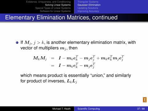
Elementary Elimination Matrices, continued

If Mj , j > k, is another elementary elimination matrix, withvector of multipliers mj , then

MkMj = I −mkeTk −mje

Tj + mke

Tkmje

Tj

= I −mkeTk −mje

Tj

which means product is essentially “union,” and similarlyfor product of inverses, LkLj





Example: Elementary Elimination Matrices

For a =

24−2

,

M1a =

1 0 0−2 1 0

1 0 1

24−2

=

200

and

M2a =

1 0 00 1 00 1/2 1

24−2

=

240





Example, continued

Note that

L1 = M−11 =

1 0 02 1 0−1 0 1

, L2 = M−12 =

1 0 00 1 00 −1/2 1

and

M1M2 =

1 0 0−2 1 0

1 1/2 1

, L1L2 =

1 0 02 1 0−1 −1/2 1





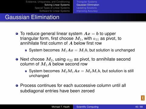
Gaussian Elimination

To reduce general linear system Ax = b to uppertriangular form, first choose M1, with a11 as pivot, toannihilate first column of A below first row

System becomes M1Ax = M1b, but solution is unchanged

Next choose M2, using a22 as pivot, to annihilate secondcolumn of M1A below second row

System becomes M2M1Ax = M2M1b, but solution is stillunchanged

Process continues for each successive column until allsubdiagonal entries have been zeroed





Gaussian Elimination, continued

Resulting upper triangular linear system

Mn−1 · · ·M1Ax = Mn−1 · · ·M1b

MAx = Mb

can be solved by back-substitution to obtain solution tooriginal linear system Ax = b

Process just described is called Gaussian elimination





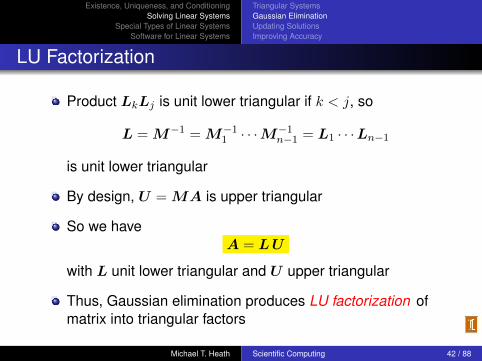
LU Factorization

Product LkLj is unit lower triangular if k < j, so

L = M−1 = M−11 · · ·M

−1n−1 = L1 · · ·Ln−1

is unit lower triangular

By design, U = MA is upper triangular

So we haveA = LU

with L unit lower triangular and U upper triangular

Thus, Gaussian elimination produces LU factorization ofmatrix into triangular factors





LU Factorization, continued

Having obtained LU factorization, Ax = b becomesLUx = b, and can be solved by forward-substitution inlower triangular system Ly = b, followed byback-substitution in upper triangular system Ux = y

Note that y = Mb is same as transformed right-hand sidein Gaussian elimination

Gaussian elimination and LU factorization are two ways ofexpressing same solution process





Example: Gaussian Elimination

Use Gaussian elimination to solve linear system

Ax =

2 4 −24 9 −3−2 −3 7

x1x2x3

=

28

10

= b

To annihilate subdiagonal entries of first column of A,

M1A =

1 0 0−2 1 0

1 0 1

2 4 −24 9 −3−2 −3 7

=

2 4 −20 1 10 1 5

,M1b =

1 0 0−2 1 0

1 0 1

28

10

=

24

12





Example, continued

To annihilate subdiagonal entry of second column of M1A,

M2M1A =

1 0 00 1 00 −1 1

2 4 −20 1 10 1 5

=

2 4 −20 1 10 0 4

= U ,

M2M1b =

1 0 00 1 00 −1 1

24

12

=

248

= Mb





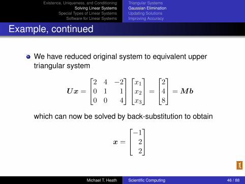
Example, continued

We have reduced original system to equivalent uppertriangular system

Ux =

2 4 −20 1 10 0 4

x1x2x3

=

248

= Mb

which can now be solved by back-substitution to obtain

x =

−122





Example, continued

To write out LU factorization explicitly,

L1L2 =

1 0 02 1 0−1 0 1

1 0 00 1 00 1 1

=

1 0 02 1 0−1 1 1

= L

so that

A =

2 4 −24 9 −3−2 −3 7

=

1 0 02 1 0−1 1 1

2 4 −20 1 10 0 4

= LU





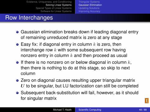
Row Interchanges

Gaussian elimination breaks down if leading diagonal entryof remaining unreduced matrix is zero at any stageEasy fix: if diagonal entry in column k is zero, theninterchange row k with some subsequent row havingnonzero entry in column k and then proceed as usualIf there is no nonzero on or below diagonal in column k,then there is nothing to do at this stage, so skip to nextcolumnZero on diagonal causes resulting upper triangular matrixU to be singular, but LU factorization can still be completedSubsequent back-substitution will fail, however, as it shouldfor singular matrix





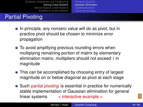
Partial Pivoting

In principle, any nonzero value will do as pivot, but inpractice pivot should be chosen to minimize errorpropagation

To avoid amplifying previous rounding errors whenmultiplying remaining portion of matrix by elementaryelimination matrix, multipliers should not exceed 1 inmagnitude

This can be accomplished by choosing entry of largestmagnitude on or below diagonal as pivot at each stage

Such partial pivoting is essential in practice for numericallystable implementation of Gaussian elimination for generallinear systems < interactive example >


http://www.cs.illinois.edu/~heath/iem/linear_equations/gaussian_elimination/




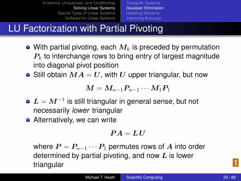
LU Factorization with Partial Pivoting

With partial pivoting, each Mk is preceded by permutationPk to interchange rows to bring entry of largest magnitudeinto diagonal pivot positionStill obtain MA = U , with U upper triangular, but now

M = Mn−1Pn−1 · · ·M1P1

L = M−1 is still triangular in general sense, but notnecessarily lower triangularAlternatively, we can write

PA = LU

where P = Pn−1 · · ·P1 permutes rows of A into orderdetermined by partial pivoting, and now L is lowertriangular





Complete Pivoting

Complete pivoting is more exhaustive strategy in whichlargest entry in entire remaining unreduced submatrix ispermuted into diagonal pivot positionRequires interchanging columns as well as rows, leadingto factorization

PAQ = LU

with L unit lower triangular, U upper triangular, and P andQ permutationsNumerical stability of complete pivoting is theoreticallysuperior, but pivot search is more expensive than for partialpivotingNumerical stability of partial pivoting is more thanadequate in practice, so it is almost always used in solvinglinear systems by Gaussian elimination





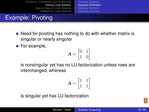
Example: Pivoting

Need for pivoting has nothing to do with whether matrix issingular or nearly singularFor example,

A =

[0 11 0

]is nonsingular yet has no LU factorization unless rows areinterchanged, whereas

A =

[1 11 1

]is singular yet has LU factorization





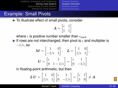
Example: Small PivotsTo illustrate effect of small pivots, consider

A =

[ε 11 1

]where ε is positive number smaller than εmachIf rows are not interchanged, then pivot is ε and multiplier is−1/ε, so

M =

[1 0−1/ε 1

], L =

[1 0

1/ε 1

],

U =

[ε 10 1− 1/ε

]=

[ε 10 −1/ε

]in floating-point arithmetic, but then

LU =

[1 0

1/ε 1

] [ε 10 −1/ε

]=

[ε 11 0

]6= A





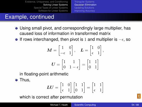
Example, continued

Using small pivot, and correspondingly large multiplier, hascaused loss of information in transformed matrixIf rows interchanged, then pivot is 1 and multiplier is −ε, so

M =

[1 0−ε 1

], L =

[1 0ε 1

],

U =

[1 10 1− ε

]=

[1 10 1

]in floating-point arithmeticThus,

LU =

[1 0ε 1

] [1 10 1

]=

[1 1ε 1

]which is correct after permutation





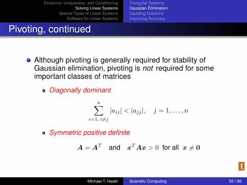
Pivoting, continued

Although pivoting is generally required for stability ofGaussian elimination, pivoting is not required for someimportant classes of matrices

Diagonally dominant

n∑i=1, i 6=j

|aij | < |ajj |, j = 1, . . . , n

Symmetric positive definite

A = AT and xTAx > 0 for all x 6= 0





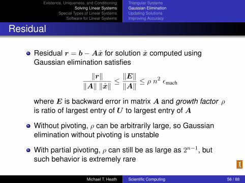
Residual

Residual r = b−Ax for solution x computed usingGaussian elimination satisfies

‖r‖‖A‖ ‖x‖

≤ ‖E‖‖A‖

≤ ρ n2 εmach

where E is backward error in matrix A and growth factor ρis ratio of largest entry of U to largest entry of A

Without pivoting, ρ can be arbitrarily large, so Gaussianelimination without pivoting is unstable

With partial pivoting, ρ can still be as large as 2n−1, butsuch behavior is extremely rare





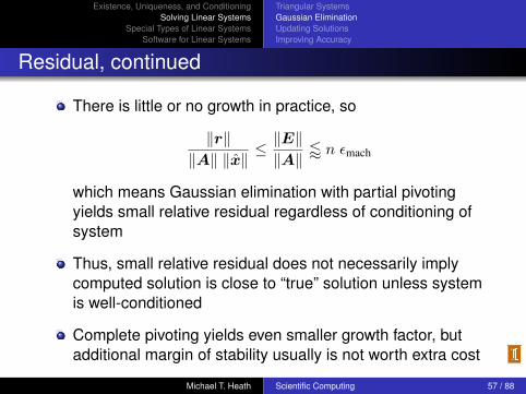
Residual, continued

There is little or no growth in practice, so

‖r‖‖A‖ ‖x‖

≤ ‖E‖‖A‖

/ n εmach

which means Gaussian elimination with partial pivotingyields small relative residual regardless of conditioning ofsystem

Thus, small relative residual does not necessarily implycomputed solution is close to “true” solution unless systemis well-conditioned

Complete pivoting yields even smaller growth factor, butadditional margin of stability usually is not worth extra cost





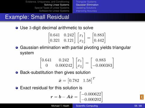
Example: Small Residual

Use 3-digit decimal arithmetic to solve[0.641 0.2420.321 0.121

] [x1x2

]=

[0.8830.442

]Gaussian elimination with partial pivoting yields triangularsystem [

0.641 0.2420 0.000242

] [x1x2

]=

[0.883−0.000383

]Back-substitution then gives solution

x =[0.782 1.58

]TExact residual for this solution is

r = b−Ax =

[−0.000622−0.000202

]Michael T. Heath Scientific Computing 58 / 88




Example, continued

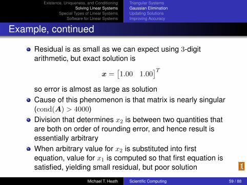
Residual is as small as we can expect using 3-digitarithmetic, but exact solution is

x =[1.00 1.00

]Tso error is almost as large as solutionCause of this phenomenon is that matrix is nearly singular(cond(A) > 4000)Division that determines x2 is between two quantities thatare both on order of rounding error, and hence result isessentially arbitraryWhen arbitrary value for x2 is substituted into firstequation, value for x1 is computed so that first equation issatisfied, yielding small residual, but poor solution





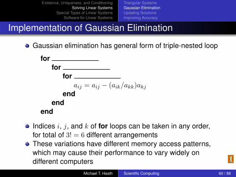
Implementation of Gaussian Elimination

Gaussian elimination has general form of triple-nested loop

forfor

foraij = aij − (aik/akk)akj

endend

end

Indices i, j, and k of for loops can be taken in any order,for total of 3! = 6 different arrangementsThese variations have different memory access patterns,which may cause their performance to vary widely ondifferent computers





Uniqueness of LU Factorization

Despite variations in computing it, LU factorization isunique up to diagonal scaling of factors

Provided row pivot sequence is same, if we have two LUfactorizations PA = LU = LU , then L−1L = UU−1 = Dis both lower and upper triangular, hence diagonal

If both L and L are unit lower triangular, then D must beidentity matrix, so L = L and U = U

Uniqueness is made explicit in LDU factorizationPA = LDU , with L unit lower triangular, U unit uppertriangular, and D diagonal





Storage Management

Elementary elimination matrices Mk, their inverses Lk,and permutation matrices Pk used in formal description ofLU factorization process are not formed explicitly in actualimplementation

U overwrites upper triangle of A, multipliers in L overwritestrict lower triangle of A, and unit diagonal of L need notbe stored

Row interchanges usually are not done explicitly; auxiliaryinteger vector keeps track of row order in original locations





Complexity of Solving Linear Systems

LU factorization requires about n3/3 floating-pointmultiplications and similar number of additions

Forward- and back-substitution for single right-hand-sidevector together require about n2 multiplications and similarnumber of additions

Can also solve linear system by matrix inversion:x = A−1b

Computing A−1 is tantamount to solving n linear systems,requiring LU factorization of A followed by n forward- andback-substitutions, one for each column of identity matrix

Operation count for inversion is about n3, three times asexpensive as LU factorization





Inversion vs. Factorization

Even with many right-hand sides b, inversion neverovercomes higher initial cost, since each matrix-vectormultiplication A−1b requires n2 operations, similar to costof forward- and back-substitutionInversion gives less accurate answer; for example, solving3x = 18 by division gives x = 18/3 = 6, but inversion givesx = 3−1 × 18 = 0.333× 18 = 5.99 using 3-digit arithmeticMatrix inverses often occur as convenient notation informulas, but explicit inverse is rarely required toimplement such formulasFor example, product A−1B should be computed by LUfactorization of A, followed by forward- andback-substitutions using each column of B





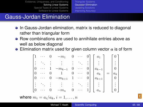
Gauss-Jordan Elimination

In Gauss-Jordan elimination, matrix is reduced to diagonalrather than triangular formRow combinations are used to annihilate entries above aswell as below diagonalElimination matrix used for given column vector a is of form

1 · · · 0 −m1 0 · · · 0...

. . ....

......

. . ....

0 · · · 1 −mk−1 0 · · · 00 · · · 0 1 0 · · · 00 · · · 0 −mk+1 1 · · · 0...

. . ....

......

. . ....

0 · · · 0 −mn 0 · · · 1

a1...

ak−1akak+1

...an

=

0...0ak0...0

where mi = ai/ak, i = 1, . . . , n





Gauss-Jordan Elimination, continued

Gauss-Jordan elimination requires about n3/2multiplications and similar number of additions, 50% moreexpensive than LU factorization

During elimination phase, same row operations are alsoapplied to right-hand-side vector (or vectors) of system oflinear equations

Once matrix is in diagonal form, components of solutionare computed by dividing each entry of transformedright-hand side by corresponding diagonal entry of matrix

Latter requires only n divisions, but this is not enoughcheaper to offset more costly elimination phase



http://www.cs.illinois.edu/~heath/iem/linear_equations/gauss_jordan/




Solving Modified Problems

If right-hand side of linear system changes but matrix doesnot, then LU factorization need not be repeated to solvenew system

Only forward- and back-substitution need be repeated fornew right-hand side

This is substantial savings in work, since additionaltriangular solutions cost only O(n2) work, in contrast toO(n3) cost of factorization





Sherman-Morrison Formula

Sometimes refactorization can be avoided even whenmatrix does change

Sherman-Morrison formula gives inverse of matrixresulting from rank-one change to matrix whose inverse isalready known

(A− uvT )−1 = A−1 + A−1u(1− vTA−1u)−1vTA−1

where u and v are n-vectors

Evaluation of formula requires O(n2) work (formatrix-vector multiplications) rather than O(n3) workrequired for inversion





Rank-One Updating of Solution

To solve linear system (A− uvT )x = b with new matrix,use Sherman-Morrison formula to obtain

x = (A− uvT )−1b

= A−1b + A−1u(1− vTA−1u)−1vTA−1b

which can be implemented by following stepsSolve Az = u for z, so z = A−1u

Solve Ay = b for y, so y = A−1b

Compute x = y + ((vTy)/(1− vTz))z

If A is already factored, procedure requires only triangularsolutions and inner products, so only O(n2) work and noexplicit inverses





Example: Rank-One Updating of Solution

Consider rank-one modification 2 4 −24 9 −3−2 −1 7

x1x2x3

=

28

10

(with 3, 2 entry changed) of system whose LU factorizationwas computed in earlier exampleOne way to choose update vectors is

u =

00−2

and v =

010

so matrix of modified system is A− uvT





Example, continued

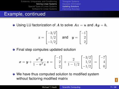
Using LU factorization of A to solve Az = u and Ay = b,

z =

−3/21/2−1/2

and y =

−122

Final step computes updated solution

x = y +vTy

1− vTzz =

−122

+2

1− 1/2

−3/21/2−1/2

=

−740

We have thus computed solution to modified systemwithout factoring modified matrix





Scaling Linear Systems

In principle, solution to linear system is unaffected bydiagonal scaling of matrix and right-hand-side vector

In practice, scaling affects both conditioning of matrix andselection of pivots in Gaussian elimination, which in turnaffect numerical accuracy in finite-precision arithmetic

It is usually best if all entries (or uncertainties in entries) ofmatrix have about same size

Sometimes it may be obvious how to accomplish this bychoice of measurement units for variables, but there is nofoolproof method for doing so in general

Scaling can introduce rounding errors if not done carefully





Example: Scaling

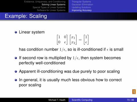
Linear system [1 00 ε

] [x1x2

]=

[1ε

]has condition number 1/ε, so is ill-conditioned if ε is small

If second row is multiplied by 1/ε, then system becomesperfectly well-conditioned

Apparent ill-conditioning was due purely to poor scaling

In general, it is usually much less obvious how to correctpoor scaling





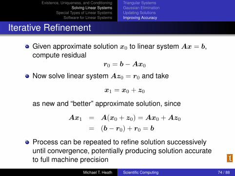
Iterative Refinement

Given approximate solution x0 to linear system Ax = b,compute residual

r0 = b−Ax0

Now solve linear system Az0 = r0 and take

x1 = x0 + z0

as new and “better” approximate solution, since

Ax1 = A(x0 + z0) = Ax0 + Az0

= (b− r0) + r0 = b

Process can be repeated to refine solution successivelyuntil convergence, potentially producing solution accurateto full machine precision





Iterative Refinement, continued

Iterative refinement requires double storage, since bothoriginal matrix and its LU factorization are required

Due to cancellation, residual usually must be computedwith higher precision for iterative refinement to producemeaningful improvement

For these reasons, iterative improvement is oftenimpractical to use routinely, but it can still be useful in somecircumstances

For example, iterative refinement can sometimes stabilizeotherwise unstable algorithm




Symmetric SystemsBanded SystemsIterative Methods

Special Types of Linear Systems

Work and storage can often be saved in solving linearsystem if matrix has special properties

Examples include

Symmetric : A = AT , aij = aji for all i, j

Positive definite : xTAx > 0 for all x 6= 0

Band : aij = 0 for all |i− j| > β, where β is bandwidth of A

Sparse : most entries of A are zero





Symmetric Positive Definite Matrices

If A is symmetric and positive definite, then LUfactorization can be arranged so that U = LT , which givesCholesky factorization

A = LLT

where L is lower triangular with positive diagonal entriesAlgorithm for computing it can be derived by equatingcorresponding entries of A and LLT

In 2× 2 case, for example,[a11 a21a21 a22

]=

[l11 0l21 l22

] [l11 l210 l22

]implies

l11 =√a11, l21 = a21/l11, l22 =

√a22 − l221





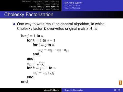
Cholesky Factorization

One way to write resulting general algorithm, in whichCholesky factor L overwrites original matrix A, is

for j = 1 to nfor k = 1 to j − 1

for i = j to naij = aij − aik · ajk

endendajj =

√ajj

for k = j + 1 to nakj = akj/ajj

endend





Cholesky Factorization, continued

Features of Cholesky algorithm for symmetric positivedefinite matrices

All n square roots are of positive numbers, so algorithm iswell definedNo pivoting is required to maintain numerical stabilityOnly lower triangle of A is accessed, and hence uppertriangular portion need not be storedOnly n3/6 multiplications and similar number of additionsare required

Thus, Cholesky factorization requires only about half workand half storage compared with LU factorization of generalmatrix by Gaussian elimination, and also avoids need forpivoting

< interactive example >Michael T. Heath Scientific Computing 79 / 88

http://www.cs.illinois.edu/~heath/iem/linear_equations/cholesky/




Symmetric Indefinite Systems

For symmetric indefinite A, Cholesky factorization is notapplicable, and some form of pivoting is generally requiredfor numerical stability

Factorization of form

PAP T = LDLT

with L unit lower triangular and D either tridiagonal orblock diagonal with 1× 1 and 2× 2 diagonal blocks, can becomputed stably using symmetric pivoting strategy

In either case, cost is comparable to that of Choleskyfactorization





Band Matrices

Gaussian elimination for band matrices differs little fromgeneral case — only ranges of loops change

Typically matrix is stored in array by diagonals to avoidstoring zero entries

If pivoting is required for numerical stability, bandwidth cangrow (but no more than double)

General purpose solver for arbitrary bandwidth is similar tocode for Gaussian elimination for general matrices

For fixed small bandwidth, band solver can be extremelysimple, especially if pivoting is not required for stability





Tridiagonal Matrices

Consider tridiagonal matrix

A =

b1 c1 0 · · · 0

a2 b2 c2. . .

...

0. . . . . . . . . 0

.... . . an−1 bn−1 cn−1

0 · · · 0 an bn

Gaussian elimination without pivoting reduces tod1 = b1for i = 2 to n

mi = ai/di−1di = bi −mici−1

endMichael T. Heath Scientific Computing 82 / 88




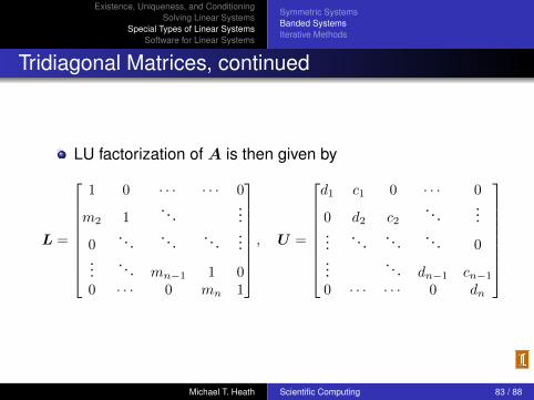
Tridiagonal Matrices, continued

LU factorization of A is then given by

L =

1 0 · · · · · · 0

m2 1. . .

...

0. . . . . . . . .

......

. . . mn−1 1 00 · · · 0 mn 1

, U =

d1 c1 0 · · · 0

0 d2 c2. . .

......

. . . . . . . . . 0...

. . . dn−1 cn−10 · · · · · · 0 dn





General Band Matrices

In general, band system of bandwidth β requires O(βn)storage, and its factorization requires O(β2n) work

Compared with full system, savings is substantial if β � n





Iterative Methods for Linear Systems

Gaussian elimination is direct method for solving linearsystem, producing exact solution in finite number of steps(in exact arithmetic)

Iterative methods begin with initial guess for solution andsuccessively improve it until desired accuracy attained

In theory, it might take infinite number of iterations toconverge to exact solution, but in practice iterations areterminated when residual is as small as desired

For some types of problems, iterative methods havesignificant advantages over direct methods

We will study specific iterative methods later when weconsider solution of partial differential equations




LINPACK and LAPACKBLAS

LINPACK and LAPACK

LINPACK is software package for solving wide variety ofsystems of linear equations, both general dense systemsand special systems, such as symmetric or banded

Solving linear systems of such fundamental importance inscientific computing that LINPACK has become standardbenchmark for comparing performance of computers

LAPACK is more recent replacement for LINPACK featuringhigher performance on modern computer architectures,including some parallel computers

Both LINPACK and LAPACK are available from Netlib





Basic Linear Algebra Subprograms

High-level routines in LINPACK and LAPACK are based onlower-level Basic Linear Algebra Subprograms (BLAS)BLAS encapsulate basic operations on vectors andmatrices so they can be optimized for given computerarchitecture while high-level routines that call them remainportableHigher-level BLAS encapsulate matrix-vector andmatrix-matrix operations for better utilization of memoryhierarchies such as cache and virtual memory with pagingGeneric Fortran versions of BLAS are available fromNetlib, and many computer vendors provide customversions optimized for their particular systems





Examples of BLAS

Level Work Examples Function1 O(n) saxpy Scalar × vector + vector

sdot Inner productsnrm2 Euclidean vector norm

2 O(n2) sgemv Matrix-vector productstrsv Triangular solutionsger Rank-one update

3 O(n3) sgemm Matrix-matrix productstrsm Multiple triang. solutionsssyrk Rank-k update

Level-3 BLAS have more opportunity for data reuse, andhence higher performance, because they perform moreoperations per data item than lower-level BLAS


scientiﬁc computing: an introductory surveyheath.cs.illinois.edu/scicomp/notes/chap02.pdf ·...

Documents