scienti c computing
TRANSCRIPT

Lecture Notes to Accompany
Scientific Computing
An Introductory SurveySecond Edition
by Michael T. Heath
Chapter 3
Linear Least Squares
Copyright c© 2001. Reproduction permitted only for
noncommercial, educational use in conjunction with the
book.
1

Method of Least Squares
Measurement errors inevitable in observational
and experimental sciences
Errors smoothed out by averaging over many
cases, i.e., taking more measurements than
strictly necessary to determine parameters of
system
Resulting system overdetermined, so usually
no exact solution
Project higher dimensional data into lower di-
mensional space to suppress irrelevant detail
Projection most conveniently accomplished by
method of least squares
2

Linear Least Squares
For linear problems, obtain overdetermined
linear system Ax = b, with m × n matrix A,
m > n
Better written Ax ∼= b, since equality usually
not exactly satisfiable when m > n
Least squares solution x minimizes squared
Euclidean norm of residual vector r = b−Ax,
minx‖r‖22 = min
x‖b−Ax‖22
3
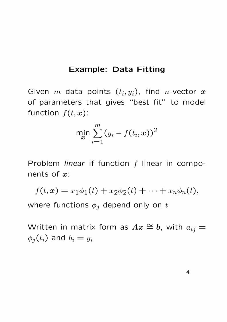
Example: Data Fitting
Given m data points (ti, yi), find n-vector x
of parameters that gives “best fit” to model
function f(t,x):
minx
m∑i=1
(yi − f(ti,x))2
Problem linear if function f linear in compo-
nents of x:
f(t,x) = x1φ1(t) + x2φ2(t) + · · ·+ xnφn(t),
where functions φj depend only on t
Written in matrix form as Ax ∼= b, with aij =
φj(ti) and bi = yi
4

Example: Data Fitting
Polynomial fitting,
f(t,x) = x1 + x2t+ x3t2 + · · ·+ xnt
n−1,
is linear, since polynomial linear in coefficients,
though nonlinear in independent variable t
Fitting sum of exponentials, with
f(t,x) = x1ex2t + · · ·+ xn−1e
xnt,
is nonlinear problem
For now, consider only linear least squares prob-
lems
5
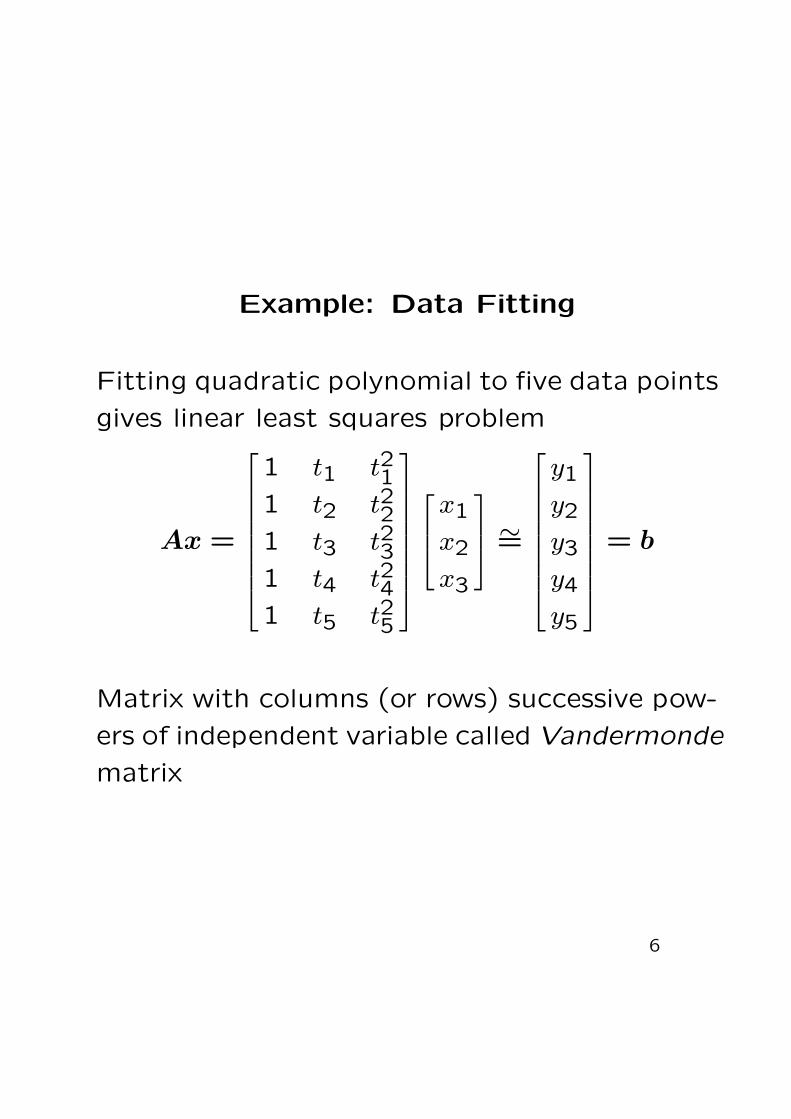
Example: Data Fitting
Fitting quadratic polynomial to five data points
gives linear least squares problem
Ax =
1 t1 t211 t2 t221 t3 t231 t4 t241 t5 t25
x1
x2
x3
∼=
y1
y2
y3
y4
y5
= b
Matrix with columns (or rows) successive pow-
ers of independent variable called Vandermonde
matrix
6

Example: Data Fitting
For data
t −1.0 −0.5 0.0 0.5 1.0y 1.0 0.5 0.0 0.5 2.0
overdetermined 5× 3 linear system is
Ax =
1 −1.0 1.0
1 −0.5 0.25
1 0.0 0.0
1 0.5 0.25
1 1.0 1.0
x1
x2
x3
∼=
1.0
0.5
0.0
0.5
2.0
= b
Solution, which we will see later how to com-
pute, is
x = [ 0.086 0.40 1.4 ]T ,
so approximating polynomial is
p(t) = 0.086 + 0.4t+ 1.4t2
7

Example: Data Fitting
Resulting curve and original data points shown
in graph:
−1 0 1
1
2
..............................................................................................................................................................................................................................................................................................................................................................................................................................................................................................................................................
......................................................................
...........................................................
.............................................................................................................................................................................................................................................................................................
•
•
•
•
•
8
Existence and Uniqueness
Linear least squares problem Ax ∼= b always
has solution
Solution unique if, and only if, columns of A
linearly independent, i.e., rank(A) = n, where
A is m× n
If rank(A) < n, then A is rank-deficient, and
solution of linear least squares problem is not
unique
For now, assume A has full column rank n
9

Normal Equations
Least squares minimizes squared Euclidean norm
‖r‖22 = rTr
of residual vector
r = b−Ax
To minimize
‖r‖22 = rTr = (b−Ax)T (b−Ax)
= bTb− 2xTATb+ xTATAx,
take derivative with respect to x and set to o,
2ATAx− 2ATb = o,
which reduces to n× n linear system
ATAx = ATb
known as system of normal equations
10

Orthogonality
Vectors v1 and v2 are orthogonal if their inner
product is zero, vT1 v2 = 0
Space spanned by columns of m× n matrix A,
span(A) = {Ax : x ∈ Rn}, is of dimension at
most n
If m > n, b generally does not lie in span(A),
so no exact solution to Ax = b
Vector y = Ax in span(A) closest to b in 2-
norm occurs when residual r = b−Ax orthog-
onal to span(A)
Thus,
o = ATr = AT (b−Ax),
or
ATAx = ATb
11

Orthogonality, continued
..........................................................................................................................................................................................................................................................................................................................................................................................................................................................................................................................................................................................................................................................................................................................................................................................................................................................................................................................................................................................................................................................................................................................................................................................................................................................................................................................................................................................................................................................................................................................................................................................................................................................................................................................................................................................................................................................................................................................................................................................................................................................................................................................................................................................................................................................
.................................................................................................................................................................................................................................................................................................................................................................................................... ..............................................................................................................................................................................................................................................................................................................................................................................................................................................................................................................................................................................................................
..............................................................................................................................
....................
.............
.............
.............
.............
.............
.............
.............
.............
.............
.............
.............
.............
.............
.............
............
θ
y = Ax
b r = b−Ax
span(A)
12

Orthogonal Projectors
Matrix P is orthogonal projector if idempotent
(P 2 = P ) and symmetric (P T = P )
Orthogonal projector onto orthogonal comple-
ment span(P )⊥ given by P⊥ = I − P
For any vector v,
v = (P + (I − P )) v = Pv + P⊥v
For least squares problem Ax ∼= b, if rank(A) =
n, then
P = A(ATA)−1AT
is orthogonal projector onto span(A), and
b = Pb+ P⊥b = Ax+ (b−Ax) = y + r
13

Pseudoinverse and Condition Number
Nonsquare m × n matrix A has no inverse in
usual sense
If rank(A) = n, pseudoinverse defined by
A+ = (ATA)−1AT
and
cond(A) = ‖A‖2 · ‖A+‖2
By convention, cond(A) =∞ if rank(A) < n
Just as condition number of square matrix mea-
sures closeness to singularity, condition num-
ber of rectangular matrix measures closeness
to rank deficiency
Least squares solution of Ax ∼= b is given by
x = A+ b14
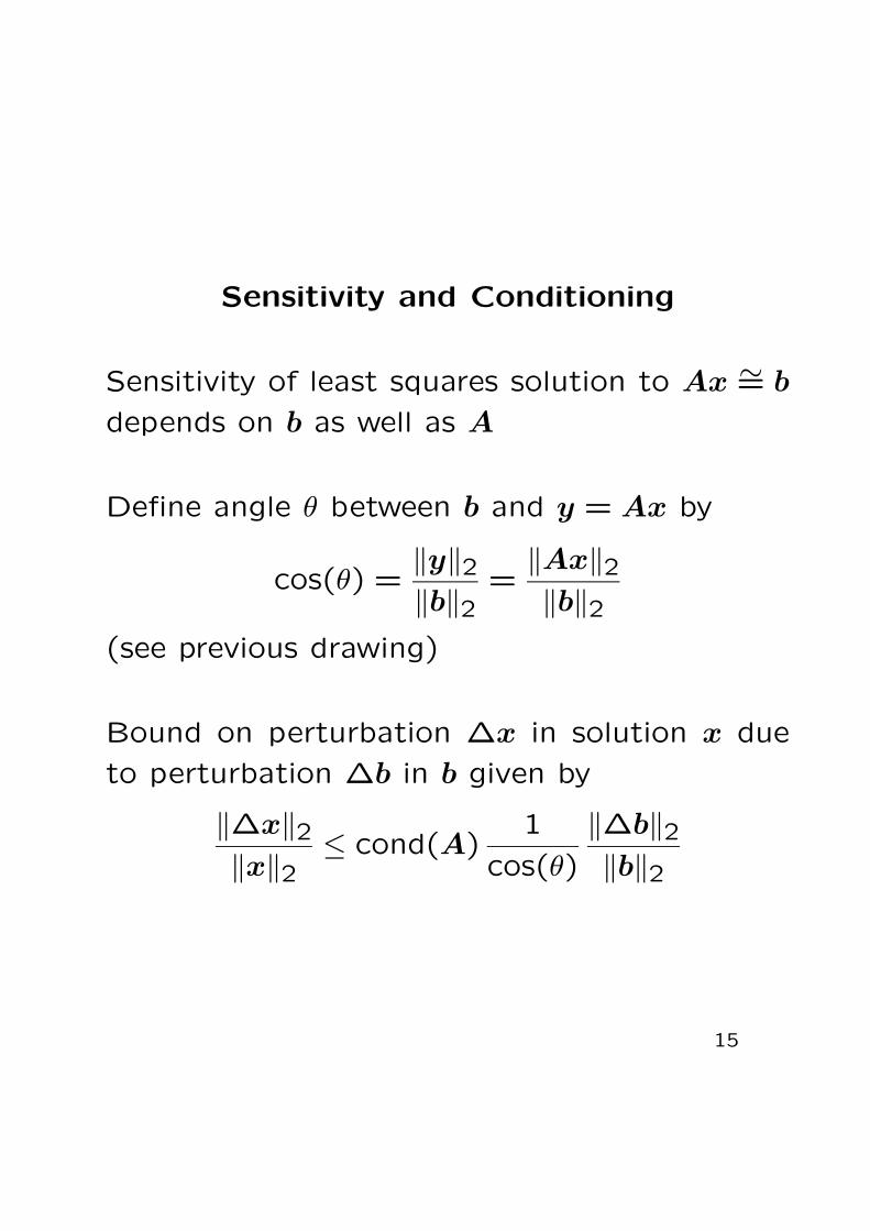
Sensitivity and Conditioning
Sensitivity of least squares solution to Ax ∼= b
depends on b as well as A
Define angle θ between b and y = Ax by
cos(θ) =‖y‖2‖b‖2
=‖Ax‖2‖b‖2
(see previous drawing)
Bound on perturbation ∆x in solution x due
to perturbation ∆b in b given by
‖∆x‖2‖x‖2
≤ cond(A)1
cos(θ)
‖∆b‖2‖b‖2
15

Sensitivity and Conditioning, cont.
Similarly, for perturbation E in matrix A,
‖∆x‖2‖x‖2
/([cond(A)]2 tan(θ) + cond(A)
) ‖E‖2‖A‖2
Condition number of least squares solution about
cond(A) if residual small, but can be squared
or arbitrarily worse for large residual
16
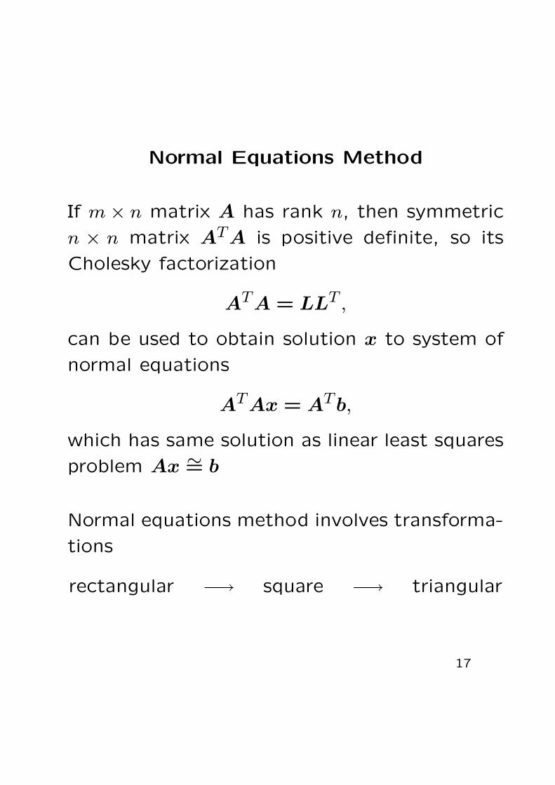
Normal Equations Method
If m× n matrix A has rank n, then symmetric
n × n matrix ATA is positive definite, so its
Cholesky factorization
ATA = LLT ,
can be used to obtain solution x to system of
normal equations
ATAx = ATb,
which has same solution as linear least squares
problem Ax ∼= b
Normal equations method involves transforma-
tions
rectangular −→ square −→ triangular
17

Example: Normal Equations Method
For polynomial data-fitting example given pre-
viously, normal equations method gives
ATA =
1 1 1 1 1
−1.0 −0.5 0.0 0.5 1.0
1.0 0.25 0.0 0.25 1.0
1 −1.0 1.0
1 −0.5 0.25
1 0.0 0.0
1 0.5 0.25
1 1.0 1.0
=
5.0 0.0 2.5
0.0 2.5 0.0
2.5 0.0 2.125
,
ATb =
1 1 1 1 1
−1.0 −0.5 0.0 0.5 1.0
1.0 0.25 0.0 0.25 1.0
1.0
0.5
0.0
0.5
2.0
=
4.0
1.0
3.25
18

Example Continued
Cholesky factorization of symmetric positive
definite matrix gives
ATA =
5.0 0.0 2.5
0.0 2.5 0.0
2.5 0.0 2.125
=
2.236 0 0
0 1.581 0
1.118 0 0.935
2.236 0 1.118
0 1.581 0
0 0 0.935
= LLT
19
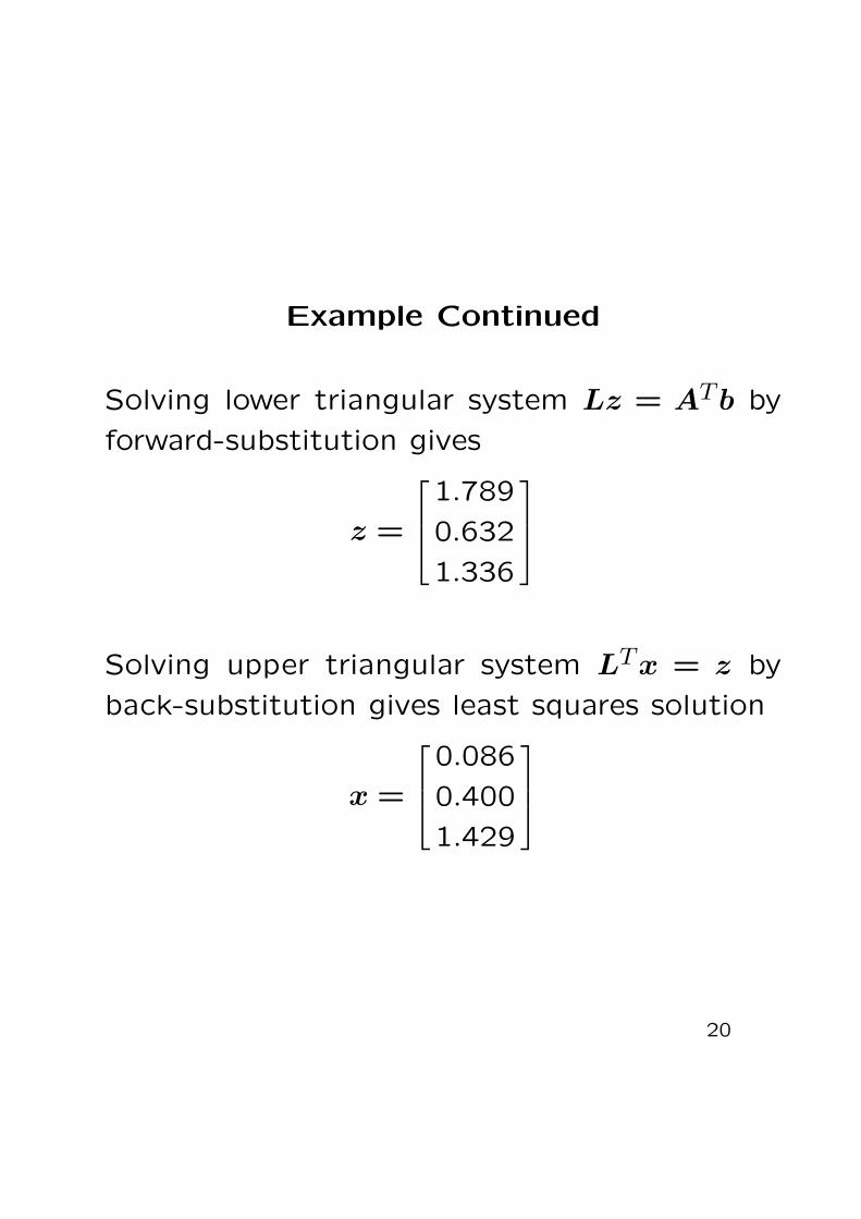
Example Continued
Solving lower triangular system Lz = ATb by
forward-substitution gives
z =
1.789
0.632
1.336
Solving upper triangular system LTx = z by
back-substitution gives least squares solution
x =
0.086
0.400
1.429
20

Shortcomings of Normal Equations
Information can be lost in forming ATA and
ATb
For example, take
A =
1 1
ε 0
0 ε
,where ε is positive number smaller than
√εmach
Then in floating-point arithmetic
ATA =
[1 + ε2 1
1 1 + ε2
]=
[1 1
1 1
],
which is singular
Sensitivity of solution also worsened, since
cond(ATA) = [cond(A)]2
21

Augmented System Method
Definition of residual and orthogonality require-
ment give (m+n)×(m+n) augmented system[I A
AT O
] [r
x
]=
[b
o
]
System not positive definite, larger than origi-
nal, and requires storing two copies of A
But allows greater freedom in choosing pivots
in computing LDLT or LU factorization
22

Augmented System Method, continued
Introducing scaling parameter α gives system[αI A
AT O
] [r/α
x
]=
[b
o
],
which allows control over relative weights of
two subsystems in choosing pivots
Reasonable rule of thumb
α = maxi,j|aij|/1000
Augmented system sometimes useful, but far
from ideal in work and storage required
23

Orthogonal Transformations
Seek alternative method that avoids numerical
difficulties of normal equations
Need numerically robust transformation that
produces easier problem
What kind of transformation leaves least squares
solution unchanged?
Square matrix Q is orthogonal if QTQ = I
Preserves Euclidean norm, since
‖Qv‖22 = (Qv)TQv = vTQTQv = vTv = ‖v‖22
Multiplying both sides of least squares problem
by orthogonal matrix does not change solution
24

Triangular Least Squares Problems
As with square linear systems, suitable target
in simplifying least squares problems is trian-
gular form
Upper triangular overdetermined (m > n) least
squares problem has form[R
O
]x ∼=
[b1
b2
],
with R n×n upper triangular and b partitioned
similarly
Residual is
‖r‖22 = ‖b1 −Rx‖22 + ‖b2‖22
25
Triangular Least Squares Problems, cont.
Have no control over second term, ‖b2‖22, but
first term becomes zero if x satisfies triangular
system
Rx = b1,
which can be solved by back-substitution
Resulting x is least squares solution, and min-
imum sum of squares is
‖r‖22 = ‖b2‖22
So strategy is to transform general least squares
problem to triangular form using orthogonal
transformation
26

QR Factorization
Given m × n matrix A, with m > n, we seek
m×m orthogonal matrix Q such that
A = Q
[R
O
],
with R n× n and upper triangular
Linear least squares problem Ax ∼= b trans-
formed into triangular least squares problem
QTAx =
[R
O
]x ∼=
[c1
c2
]= QTb,
which has same solution, since ‖r‖22 =
‖b−Ax‖22 = ‖b−Q[R
O
]x‖22 = ‖QTb−
[R
O
]x‖22
= ‖c1 −Rx‖22 + ‖c2‖22because orthogonal transformation preserves
Euclidean norm
27

Orthogonal Bases
Partition m×m orthogonal matrix Q = [Q1 Q2],
with Q1 m× n
Then
A = Q
[R
O
]= [Q1 Q2]
[R
O
]= Q1R
is reduced QR factorization of A
Columns of Q1 are orthonormal basis for span(A),
and columns of Q2 are orthonormal basis for
span(A)⊥
Q1QT1 is orthogonal projector onto span(A)
Solution to least squares problem Ax ∼= b given
by solution to square system
QT1Ax = Rx = c1 = QT1b
28
QR Factorization
To compute QR factorization of m× n matrix
A, with m > n, annihilate subdiagonal entries
of successive columns of A, eventually reach-
ing upper triangular form
Similar to LU factorization by Gaussian elim-
ination, but uses orthogonal transformations
instead of elementary elimination matrices
Possible methods include
• Householder transformations
• Givens rotations
• Gram-Schmidt orthogonalization
29

Householder Transformations
Householder transformation has form
H = I − 2vvT
vTvfor nonzero vector v
H = HT = H−1, so H is orthogonal and sym-
metric
Given vector a, choose v so that
Ha =
α
0...
0
= α
1
0...
0
= αe1
Substituting into formula for H, can take
v = a− αe1
and α = ±‖a‖2, with sign chosen to avoid can-
cellation30

Example: Householder Transformation
Let a = [ 2 1 2 ]T
By foregoing recipe,
v = a− αe1 =
2
1
2
− α1
0
0
=
2
1
2
−α0
0
,where α = ±‖a‖2 = ±3
Since a1 positive, choosing negative sign for α
avoids cancellation
Thus, v =
2
1
2
−−3
0
0
=
5
1
2
To confirm that transformation works,
Ha = a− 2vTa
vTvv =
2
1
2
− 215
30
5
1
2
=
−3
0
0
31
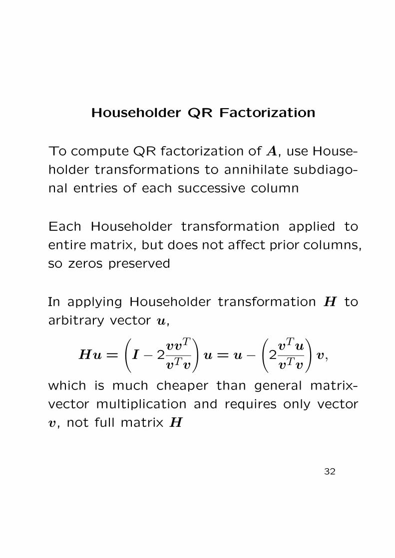
Householder QR Factorization
To compute QR factorization of A, use House-
holder transformations to annihilate subdiago-
nal entries of each successive column
Each Householder transformation applied to
entire matrix, but does not affect prior columns,
so zeros preserved
In applying Householder transformation H to
arbitrary vector u,
Hu =
(I − 2
vvT
vTv
)u = u−
(2vTu
vTv
)v,
which is much cheaper than general matrix-
vector multiplication and requires only vector
v, not full matrix H
32
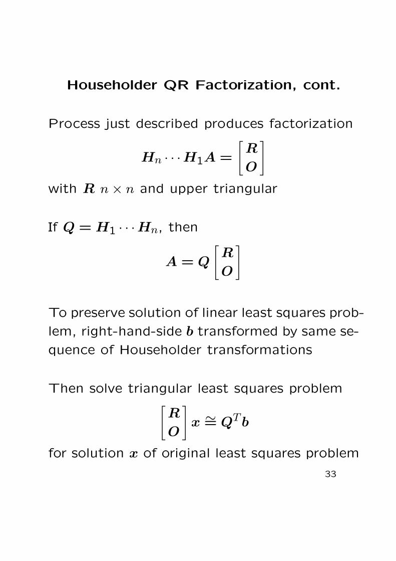
Householder QR Factorization, cont.
Process just described produces factorization
Hn · · ·H1A =
[R
O
]with R n× n and upper triangular
If Q = H1 · · ·Hn, then
A = Q
[R
O
]
To preserve solution of linear least squares prob-
lem, right-hand-side b transformed by same se-
quence of Householder transformations
Then solve triangular least squares problem[R
O
]x ∼= QTb
for solution x of original least squares problem
33

Householder QR Factorization, cont.
For solving linear least squares problem, prod-
uct Q of Householder transformations need not
be formed explicitly
R can be stored in upper triangle of array ini-
tially containing A
Householder vectors v can be stored in (now
zero) lower triangular portion of A (almost)
Householder transformations most easily ap-
plied in this form anyway
34
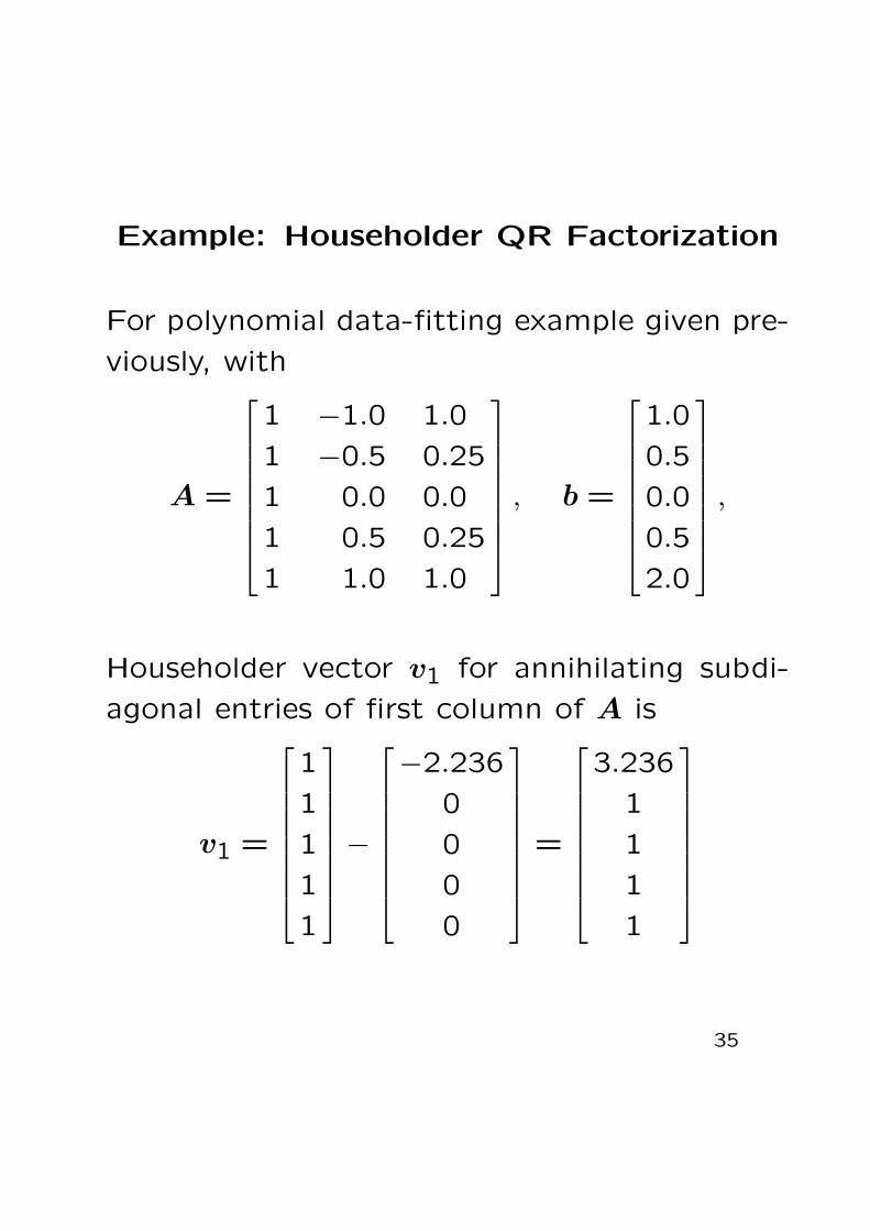
Example: Householder QR Factorization
For polynomial data-fitting example given pre-
viously, with
A =
1 −1.0 1.0
1 −0.5 0.25
1 0.0 0.0
1 0.5 0.25
1 1.0 1.0
, b =
1.0
0.5
0.0
0.5
2.0
,
Householder vector v1 for annihilating subdi-
agonal entries of first column of A is
v1 =
1
1
1
1
1
−
−2.236
0
0
0
0
=
3.236
1
1
1
1
35

Example Continued
Applying resulting Householder transformation
H1 yields transformed matrix and right-hand
side
H1A =
−2.236 0 −1.118
0 −0.191 −0.405
0 0.309 −0.655
0 0.809 −0.405
0 1.309 0.345
H1b =
−1.789
−0.362
−0.862
−0.362
1.138
36

Example Continued
Householder vector v2 for annihilating subdi-
agonal entries of second column of H1A is
v2 =
0
−0.191
0.309
0.809
1.309
−
0
1.581
0
0
0
=
0
−1.772
0.309
0.809
1.309
Applying resulting Householder transformation
H2 yields
H2H1A =
−2.236 0 −1.118
0 1.581 0
0 0 −0.725
0 0 −0.589
0 0 0.047
37

Example Continued
H2H1b =
−1.789
0.632
−1.035
−0.816
0.404
Householder vector v3 for annihilating subdi-
agonal entries of third column of H2H1A is
v3 =
0
0
−0.725
−0.589
0.047
−
0
0
0.935
0
0
=
0
0
−1.660
−0.589
0.047
38

Example Continued
Applying resulting Householder transformation
H3 yields
H3H2H1A =
−2.236 0 −1.118
0 1.581 0
0 0 0.935
0 0 0
0 0 0
H3H2H1b =
−1.789
0.632
1.336
0.026
0.337
Now solve upper triangular system Rx = c1 by
back-substitution to obtain
x = [ 0.086 0.400 1.429 ]T
39

Givens Rotations
Givens rotations introduce zeros one at a time
Given vector [ a1 a2 ]T , choose scalars c and
s so that [c s
−s c
] [a1
a2
]=
[α
0
],
with c2 + s2 = 1, or equivalently, α =√a2
1 + a22
Previous equation can be rewritten[a1 a2
a2 −a1
] [c
s
]=
[α
0
]
Gaussian elimination yields triangular system[a1 a2
0 −a1 − a22/a1
] [c
s
]=
[α
−αa2/a1
]
40

Givens Rotations, continued
Back-substitution then gives
s =αa2
a21 + a2
2
, c =αa1
a21 + a2
2
Finally, c2 + s2 = 1, or α =√a2
1 + a22, implies
c =a1√
a21 + a2
2
, s =a2√
a21 + a2
2
41

Example: Givens Rotation
Let a = [ 4 3 ]T
Computing cosine and sine,
c =a1√
a21 + a2
2
=4
5= 0.8
s =a2√
a21 + a2
2
=3
5= 0.6
Rotation given by
G =
[c s
−s c
]=
[0.8 0.6
−0.6 0.8
]
To confirm that rotation works,
Ga =
[0.8 0.6
−0.6 0.8
] [4
3
]=
[5
0
]
42

Givens QR Factorization
To annihilate selected component of vector inn dimensions, rotate target component withanother component
1 0 0 0 0
0 c 0 s 0
0 0 1 0 0
0 −s 0 c 0
0 0 0 0 1
a1
a2
a3
a4
a5
=
a1
α
a3
0
a5
Reduce matrix to upper triangular form usingsequence of Givens rotations
Each rotation orthogonal, so their product isorthogonal, producing QR factorization
Straightforward implementation of Givensmethod requires about 50% more work thanHouseholder method, and also requires morestorage, since each rotation requires two num-bers, c and s, to define it
43

Gram-Schmidt Orthogonalization
Given vectors a1 and a2, can determine or-
thonormal vectors q1 and q2 with same span
by orthogonalizing one vector against other:
....................................................
....................................................
....................................................
....................................................
....................................................
....................................................
....................................................
....................................................
................................................................................................
....................................................
....................................................
....................................................
....................................................
....................................................
...............................................................
................................................................................................................................................................................................................................................................................................................................................................................................................................................
...................................................................................................................................................................................................................................................................................................................................
........................................................................................................................................................................................
......................................................................
.............................................................................................................................................................................................
a1a2
q1q2
a2 − (qT1a2)q1
for k = 1 to n
qk = akfor j = 1 to k − 1
rjk = qTj akqk = qk − rjkqj
end
rkk = ‖qk‖2qk = qk/rkk
end
44

Modified Gram-Schmidt
Classical Gram-Schmidt procedure often suf-fers loss of orthogonality in finite-precision
Also, separate storage is required for A, Q, andR, since original ak needed in inner loop, so qkcannot overwrite columns of A
Both deficiencies improved by modified Gram-Schmidt procedure, with each vector orthogo-nalized in turn against all subsequent vectorsso qk can overwrite ak:
for k = 1 to n
rkk = ‖ak‖2qk = ak/rkkfor j = k + 1 to n
rkj = qTk ajaj = aj − rkjqk
end
end
45
Rank Deficiency
If rank(A) < n, then QR factorization still ex-
ists, but yields singular upper triangular factor
R, and multiple vectors x give minimum resid-
ual norm
Common practice selects minimum residual so-
lution x having smallest norm
Can be computed by QR factorization with
column pivoting or by singular value decom-
position (SVD)
Rank of matrix often not clear cut in practice,
so relative tolerance used to determine rank
46

Example: Near Rank Deficiency
Consider 3× 2 matrix
A =
0.641 0.242
0.321 0.121
0.962 0.363
Computing QR factorization,
R =
[1.1997 0.4527
0 0.0002
]
R extremely close to singular (exactly singular
to 3-digit accuracy of problem statement)
If R used to solve linear least squares prob-
lem, result is highly sensitive to perturbations
in right-hand side
For practical purposes, rank(A) = 1 rather
than 2, because columns nearly linearly depen-
dent47
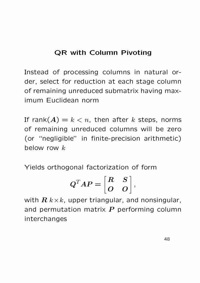
QR with Column Pivoting
Instead of processing columns in natural or-
der, select for reduction at each stage column
of remaining unreduced submatrix having max-
imum Euclidean norm
If rank(A) = k < n, then after k steps, norms
of remaining unreduced columns will be zero
(or “negligible” in finite-precision arithmetic)
below row k
Yields orthogonal factorization of form
QTAP =
[R S
O O
],
with R k×k, upper triangular, and nonsingular,
and permutation matrix P performing column
interchanges
48

QR with Column Pivoting, cont.
Basic solution to least squares problem Ax ∼= b
can now be computed by solving triangular sys-
tem Rz = c1, where c1 contains first k com-
ponents of QTb, and then taking
x = P
[z
o
]
Minimum-norm solution can be computed, if
desired, at expense of additional processing to
annihilate S
rank(A) usually unknown, so rank determined
by monitoring norms of remaining unreduced
columns and terminating factorization when
maximum value falls below tolerance
49

Singular Value Decomposition
Singular value decomposition (SVD) of m × nmatrix A has form
A = UΣV T ,
where U is m×m orthogonal matrix, V is n×northogonal matrix, and Σ is m × n diagonal
matrix, with
σij =
{0 for i 6= jσi ≥ 0 for i = j
Diagonal entries σi, called singular values of A,
usually ordered so that σ1 ≥ σ2 ≥ · · · ≥ σn
Columns ui of U and vi of V called left and
right singular vectors
50

Example: SVD
SVD of
A =
1 2 3
4 5 6
7 8 9
10 11 12
given by UΣV T =.141 .825 −.420 −.351
.344 .426 .298 .782
.547 .0278 .664 −.509
.750 −.371 −.542 .0790
25.5 0 0
0 1.29 0
0 0 0
0 0 0
.504 .574 .644
−.761 −.057 .646
.408 −.816 .408
51
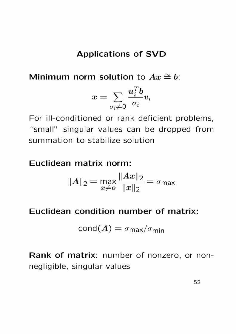
Applications of SVD
Minimum norm solution to Ax ∼= b:
x =∑σi 6=0
uTi b
σivi
For ill-conditioned or rank deficient problems,
“small” singular values can be dropped from
summation to stabilize solution
Euclidean matrix norm:
‖A‖2 = maxx 6=o
‖Ax‖2‖x‖2
= σmax
Euclidean condition number of matrix:
cond(A) = σmax/σmin
Rank of matrix: number of nonzero, or non-
negligible, singular values
52
Pseudoinverse
Define pseudoinverse of scalar σ to be 1/σ if
σ 6= 0, zero otherwise
Define pseudoinverse of (possibly rectangular)
diagonal matrix by transposing and taking scalar
pseudoinverse of each entry
Then pseudoinverse of general real m×n matrix
A given by
A+ = V Σ+UT
Pseudoinverse always exists whether or not ma-
trix is square or has full rank
If A is square and nonsingular, then A+ = A−1
In all cases, minimum-norm solution to Ax ∼= b
is given by A+ b
53

Orthogonal Bases
Columns of U corresponding to nonzero singu-
lar values form orthonormal basis for span(A)
Remaining columns of U form orthonormal
basis for orthogonal complement span(A)⊥
Columns of V corresponding to zero singular
values form orthonormal basis for null space of
A
Remaining columns of V form orthonormal
basis for orthogonal complement of null space
54

Lower-Rank Matrix Approximation
Another way to write SVD:
A = UΣV T = σ1E1 + σ2E2 + · · ·+ σnEn,
with Ei = uivTi
Ei has rank 1 and can be stored using onlym+ n storage locations
Product Eix can be formed using only m + n
multiplications
Condensed approximation to A obtained byomitting from summation terms correspondingto small singular values
Approximation using k largest singular valuesis closest matrix of rank k to A
Approximation is useful in image processing,data compression, information retrieval, cryp-tography, etc.
55

Total Least Squares
Ordinary least squares applicable when right
hand side b subject to random error but matrix
A known accurately
When all data, including A, subject to error,
then total least squares more appropriate
Total least squares minimizes orthogonal dis-
tances, rather than vertical distances, between
model and data
Total least squares solution can be computed
from SVD of [A, b]
56

Comparison of Methods
Forming normal equations matrix ATA requires
about n2m/2 multiplications, and solving re-
sulting symmetric linear system requires about
n3/6 multiplications
Solving least squares problem using Householder
QR factorization requires about mn2 − n3/3
multiplications
If m ≈ n, two methods require about same
amount of work
If m� n, Householder QR requires about twice
as much work as normal equations
Cost of SVD proportional to mn2 + n3, with
proportionality constant ranging from 4 to 10,
depending on algorithm used
57

Comparison of Methods, continued
Normal equations method produces solution
whose relative error is proportional to [cond(A)]2
Required Cholesky factorization can be expected
to break down if cond(A) ≈ 1/√εmach or worse
Householder method produces solution whose
relative error is proportional to
cond(A) + ‖r‖2 [cond(A)]2,
which is best possible, since this is inherent
sensitivity of solution to least squares problem
Householder method can be expected to break
down (in back-substitution phase) only if
cond(A) ≈ 1/εmach
or worse
58

Comparison of Methods, continued
Householder is more accurate and more broadly
applicable than normal equations
These advantages may not be worth additional
cost, however, when problem is sufficiently well
conditioned that normal equations provide ad-
equate accuracy
For rank-deficient or nearly rank-deficient prob-
lem, Householder with column pivoting can pro-
duce useful solution when normal equations
method fails outright
SVD is even more robust and reliable than
Householder, but substantially more expensive
59