Applied Mathematics 205

Advanced Scientific Computing:Numerical Methods

Lecturer: Chris H. Rycroft

Logistics

Lectures: Tuesday/Thursday, 10 AM–11:30 AM60 Oxford Street, Room 330

Email: chr@seas.harvard.edu

Course website:http://iacs-courses.seas.harvard.edu/course/am205

We will use Piazza for questions and discussionhttp://www.piazza.com

(see AM205 website for link to Piazza page)

Logistics

My office: Pierce Hall, Room 305

Office hours: Thursday, 3:00 PM–4:30 PM (starting today)

TFs: Nick Boffi (boffi@g.harvard.edu)Jinsoo Kim (jinsookim@g.harvard.edu)

Doodle poll for office hours:http://doodle.com/poll/g3w3rrfra55ztkim

(Also linked off the website front page)

Prerequisites

I Calculus

I Linear algebra

I Course will touch on PDEs, but no detailed knowledgerequired (i.e. you don’t need to have taken a PDE course)

I Some programming experience

Programming languages

Python will be used for the in-class demonstrations. Why Python?

I Freely available, widely used, and versatile

I Interpreted language, good for small tasks without the needfor compilation

I Good linear algebra support via NumPy and SciPy extensions1

I Good visualization support via Matplotlib2

1http://www.numpy.org and http://www.scipy.org/2http://www.matplotlib.org

Programming languages

There are many other languages that are widely used for scientificcomputing:

Interpreted languages: MATLAB, Julia, Perl, GNU Octave

Compiled languages: Fortran, C/C++

You can complete the assignments in any language of your choice,as long as it is easy for the teaching staff to run your code—forlanguages not listed here, please check with the teaching staff.

Note that MATLAB shares many similarities with Python, andmany numerical functions have identical names (e.g. linspace,eig), making it easy to follow the in-class examples.

Programming languages: assigment 0

Assignment 0 is posted on the course website.

Assignment 0 provides some problems to indicate the expectedlevel of programming familiarity for the outset of the course.

Asssignment 0 is not assessed, but it should either:

I confirm that you are already sufficiently familiar with Python(or MATLAB, C++, etc.)

I indicate that you need to get some programming assistance

Also, contact me or TFs regarding programming questions (Piazzais useful for these types of questions).

Python tutorial

Nick and Jinsoo will organize a tutorial on Python on WednesdaySep 9th in the afternoon.

It will cover the basics of Python programming, particularly aimedat those who have some limited experience coding in otherlanguages.

Syllabus (part 1)

0. Overview of Scientific Computing

1. Data Fitting1.1 Polynomial interpolation1.2 Linear least squares fitting1.3 Nonlinear least squares

2. Numerical Linear Algebra2.1 LU and Cholesky factorizations2.2 QR factorization, singular value decomposition

3. Numerical Calculus and Differential Equations3.1 Numerical differentiation, numerical integration3.2 ODEs, forward/backward Euler, Runge–Kutta schemes3.3 Lax equivalence theorem, stability regions for ODE solvers3.4 Boundary value problems, PDEs, finite difference method

Syllabus

4. Nonlinear Equations and Optimization4.1 Root finding, univariate and multivariate cases4.2 Necessary conditions for optimality4.3 Survey of optimization algorithms

5. Eigenvalue problems5.1 QR algorithm5.2 Power method, inverse iteration5.3 Lanczos algorithm, Arnoldi algorithm

(Similar to previous years by Chris Rycroft, David Knezevic, andEfthimios Kaxiras, with minor adjustments. Notes from 2013,2014, & 2015 still online. Videos from 2013 still online.)

Assessment

I 60% – Five homework assignments with equal weighting

I 10% – One take-home midterm exam

I 30% – Final project

Assessment: homework

The focus of the homework assignments will be on themathematical theory, but will involve significant programming.

Homework will be due on Fridays – submit a written report andsource code via the Harvard Canvas page (linked from mainwebsite). The written report should be individually submitted aseither a PDF or Word document.

Late homework will be evaluated on a case-by-case basis.

Deadlines are Sep 23, Oct 7, Oct 21, Nov 4, Dec 2.

Writing style and LATEX

Assignments will be written in LATEX, which is an excellent platformfor writing scientific documents and equations. While completelyoptional, we encourage you to try and use LATEX for yourassignments. The teaching staff are all happy to talk further.

LATEX is free and available on all major computing platforms. UsingLATEX involves writing a file in a simple markup language, which isthen compiled into a PDF or PostScript file. See the excellent NotSo Short Introduction to LATEX 2ε

3 for more information.

The original LATEX files for the homework assignments will beposted to the website for reference.

3https://tobi.oetiker.ch/lshort/lshort.pdf

Assessment: code for homework

Code should be written clearly and commented thoroughly.

In-class examples will try to adhere to this standard.

The TFs should be able to easily run your code and reproduce yourfigures.

Homework assignments: collaboration policy

Discussion and the exchange of ideas are essential to doingacademic work. For assignments in this course, you are encouragedto consult with your classmates as you work on problem sets.However, after discussion with peers, make sure that you can workthrough the problem sets yourself and ensure that any answers yousubmit for evaluation are written in your own words.

In addition, you must cite any books, articles, websites, lectures,etc. that have helped you with your work using appropriatecitation practices. Similarly, you must list the names of studentswith whom you have collaborated on problem sets.

Assessment: midterm exam

I Worth 10% of overall grade

I Scheduled for Thursday November 10th

I Take-home exam with 48 hours to complete4

I No discussion or collaboration permitted

4Note that November 11th is Veterans Day, which is a university holiday,but only for staff. Special dispensations will be made for any students whoprefer not to take the exam on this date.

Assessment: final project

The goal of this course is to get you to be a responsible,productive user of numerical algorithms for real-world applications

The best way to demonstrate this is in your final project, worth30%, to be completed in a group of two or three students5

I Use concepts/methods related to the course to solve aproblem of interest to your group

I Project proposal in the form of an oral meeting with theteaching staff due by 6 PM on Thursday November 17th

I Project due at 5 PM on Wednesday Dec 14th.

I Submit a report and associated code

I Possible option to present a poster at the CS Fall postersession

5Single person projects may be allowed with instructor permission.

Textbooks

Most relevant textbook is Scientific Computing: An IntroductorySurvey by Michael T. Heath

Textbooks

I A. Greenbaum and T. P. Chartier. Numerical Methods:Design, Analysis and Computer Implementation of Algorithms.Princeton University Press, 2012.

I C. Moler. Numerical Computing with MATLAB. SIAM, 2004.

I L. N. Trefethen and D. Bau. Numerical Linear Algebra.SIAM, 1997.

I W. H. Press, S. A. Teukolsky, W. T. Vetterling,B. P. Flannery. Numerical Recipes: The Art of ScientificComputing. Cambridge University Press, 2007.

I L. R. Scott. Numerical Analysis. Princeton University Press,2011.

I E. Suli, D. F. Mayers. An Introduction to Numerical Analysis.Cambridge University Press, 2003.

I J. Demmel. Applied Numerical Linear Algebra. SIAM, 1997.

Applied Mathematics 205

Unit 0: Overview of Scientific Computing

Lecturer: Chris H. Rycroft

Scientific Computing

Computation is now recognized as the “third pillar” of science(along with theory and experiment)

Why?

I Computation allows us to explore theoretical/mathematicalmodels when those models can’t be solved analytically

I This is usually the case for real-world problems

I e.g. Navier–Stokes equation model fluid flow, but exactsolutions only exist in a few simple cases

I Advances in algorithms and hardware over the past 50 yearshave steadily increased the prominence of scientific computing

What is Scientific Computing?

Scientific computing (SC) is closely related to numerical analysis(NA)

“Numerical analysis is the study of algorithms for the problems ofcontinuous mathematics”Nick Trefethen, SIAM News, 1992.

NA is the study of these algorithms, while SC emphasizes theirapplication to practical problems

Continuous mathematics: algorithms involving real (or complex)numbers, as opposed to integers

NA/SC are quite distinct from Computer Science, which usuallyfocuss on discrete mathematics (e.g. graph theory or cryptography)

Scientific Computing: Cosmology

Cosmological simulations allow researchers to test theories ofgalaxy formation

(cosmicweb.uchicago.edu)

Scientific Computing: Biology

Scientific computing is now crucial in molecular biology, e.g.protein folding (cnx.org)

Or statistical analysis of gene expression

(Markus Ringner, Nature Biotechnology, 2008)

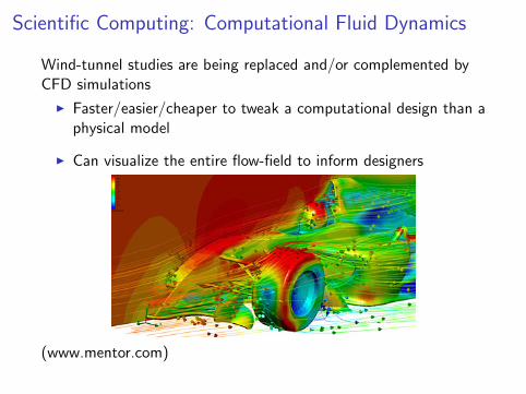
Scientific Computing: Computational Fluid Dynamics

Wind-tunnel studies are being replaced and/or complemented byCFD simulations

I Faster/easier/cheaper to tweak a computational design than aphysical model

I Can visualize the entire flow-field to inform designers

(www.mentor.com)

Scientific Computing: Geophysics

In geophysics we only have data on the earth’s surface

Computational simulations allow us to test models of the interior

(www.tacc.utexas.edu)

What is Scientific Computing?

NA and SC have been important subjects for centuries, eventhough the names we use today are relatively recent.

One of the earliest examples: calculation of π. Early values:

I Babylonians: 31/8

I Egyptians: 4(8/9)2 ≈ 3.16049

I Quote from the Old Testament: “And he made the moltensea of ten cubits from brim to brim, round in compass, andthe height thereof was five cubits; and a line of thirty cubitsdid compass it round about” – 1 Kings 7:23. Implies π ≈ 3.

What is Scientific Computing?

Archimedes’ (287–212 BC) approximation of π used a recursionrelation for the area of a polygon

Archimedes calculated that 3 1071 < π < 3 1

7 , an interval of 0.00201

What is Scientific Computing?

Key numerical analysis ideas captured by Archimedes:

I Approximate an infinite/continuous process (area integration)by a finite/discrete process (polygon perimeter)

I Error estimate (3 1071 < π < 3 1

7 ) is just as important as theapproximation itself

What is Scientific Computing?

We will encounter algorithms from many great mathematicians:Newton, Gauss, Euler, Lagrange, Fourier, Legendre, Chebyshev,. . . .

They were practitioners of scientific computing (using “handcalculations”), e.g. for astronomy, optics, mechanics, . . . .

Very interested in accurate and efficient methods since handcalculations are so laborious.

Calculating π more accurately

Jame Gregory (1638–1675) discovers the arctangent series

tan−1 x = x − x3

3+

x5

5− x7

7+ . . . .

Putting x = 1 gives

π

4= 1− 1

3+

1

5− 1

7+ . . . ,

but this is formula converges very slowly.

Formula of John Machin (1680–1752)

If tanα = 1/5, then

tan 2α =2 tanα

1− tan2 α=

5

12=⇒ tan 4α =

2 tan 2α

1− tan2 2α=

120

119.

This very close to one, and hence

tan(

4α− π

4

)=

tan 4α− 1

1 + tan 4α=

1

239.

Taking the arctangent of both sides gives the Machin formula

π

4= 4 tan−1 1

5− tan−1 1

239,

which gives much faster convergence.

The arctangent digit hunters

1706 John Machin, 100 digits1719 Thomas de Lagny, 112 digits1739 Matsunaga Ryohitsu, 50 digits1794 Georg von Vega, 140 digits1844 Zacharias Dase, 200 digits1847 Thomas Clausen, 248 digits1853 William Rutherford, 440 digits1876 William Shanks, 707 digits

A short poem to Shanks6

Seven hundred sevenShanks did state

Digits of π he would calculateAnd none can denyIt was a good try

But he erred in five twenty eight!

6If you would like more poems and facts about π, see slides from TheWonder of Pi , a public lecture Chris gave at Amherst Town Library on 3/14/16.

Scientific Computing vs. Numerical Analysis

SC and NA are closely related, each field informs the other

Emphasis of AM205 is Scientific Computing

We focus on knowledge required for you to be a responsibleuser of numerical methods for practical problems

Sources of Error in Scientific Computing

There are several sources of error in solving real-world ScientificComputing problems

Some are beyond our control, e.g. uncertainty in modelingparameters or initial conditions

Some are introduced by our numerical approximations:

I Truncation/discretization: We need to make approximations inorder to compute (finite differences, truncate infinite series...)

I Rounding: Computers work with finite precision arithmetic,which introduces rounding error

Sources of Error in Scientific Computing

It is crucial to understand and control the error introduced bynumerical approximation, otherwise our results might be garbage

This is a major part of Scientific Computing, called error analysis

Error analysis became crucial with advent of modern computers:larger scale problems =⇒ more accumulation of numerical error

Most people are more familiar with rounding error, butdiscretization error is usually far more important in practice

Discretization Error vs. Rounding Error

Consider finite difference approximation to f ′(x):

fdiff(x ; h) ≡ f (x + h)− f (x)

h

From Taylor series

f (x + h) = f (x) + hf ′(x) + f ′′(θ)h2/2, where θ ∈ [x , x + h]

we see that

fdiff(x ; h) =f (x + h)− f (x)

h= f ′(x) + f ′′(θ)h/2.

Suppose |f ′′(θ)| ≤ M, then bound on discretization error is

|f ′(x)− fdiff(x ; h)| ≤ Mh/2.

Discretization Error vs. Rounding Error

But we can’t compute fdiff(x ; h) in exact arithmetic

Let fdiff(x ; h) denote finite precision approximation of fdiff(x ; h)

Numerator of fdiff introduces rounding error . ε|f (x)|(on modern computers ε ≈ 10−16, will discuss this shortly)

Hence we have the rounding error

|fdiff(x ; h)− fdiff(x ; h)| .

∣∣∣∣ f (x + h)− f (x)

h− f (x + h)− f (x) + εf (x)

h

∣∣∣∣≤ ε|f (x)|/h

Discretization Error vs. Rounding Error

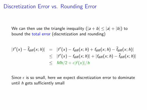
We can then use the triangle inequality (|a + b| ≤ |a|+ |b|) tobound the total error (discretization and rounding)

|f ′(x)− fdiff(x ; h)| = |f ′(x)− fdiff(x ; h) + fdiff(x ; h)− fdiff(x ; h)|≤ |f ′(x)− fdiff(x ; h)|+ |fdiff(x ; h)− fdiff(x ; h)|≤ Mh/2 + ε|f (x)|/h

Since ε is so small, here we expect discretization error to dominateuntil h gets sufficiently small

Discretization Error vs. Rounding Error

For example, consider f (x) = exp(5x), f.d. error at x = 1 asfunction of h:

10−15

10−10

10−5

10−6

10−4

10−2

100

102

104

h

Total error

Truncation dominantRounding dominant

Exercise: Use calculus to find local minimum of error bound as afunction of h to see why minimum occurs at h ≈ 10−8

Discretization Error vs. Rounding Error

Note that this in this finite difference example, we observe errorgrowth due to rounding as h→ 0

This is a nasty situation, due to factor of h on the denominator inthe error bound

A more common situation (that we’ll see in Unit 1, for example) isthat the error plateaus at around ε due to rounding error

Discretization Error vs. Rounding Error

Error plateau:

0 5 10 15 2010

−16

10−14

10−12

10−10

10−8

10−6

10−4

10−2

100

102

N

Error

Convergence plateau at ǫTruncation dominant

Absolute vs. Relative Error

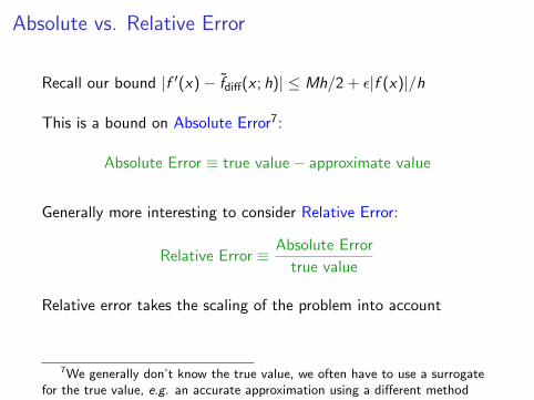
Recall our bound |f ′(x)− fdiff(x ; h)| ≤ Mh/2 + ε|f (x)|/h

This is a bound on Absolute Error7:

Absolute Error ≡ true value− approximate value

Generally more interesting to consider Relative Error:

Relative Error ≡ Absolute Error

true value

Relative error takes the scaling of the problem into account

7We generally don’t know the true value, we often have to use a surrogatefor the true value, e.g. an accurate approximation using a different method

Absolute vs. Relative Error

For our finite difference example, plotting relative error justrescales the error values

10−15

10−10

10−5

10−8

10−6

10−4

10−2

100

102

h

Relative error

Sidenote: Convergence plots

We have shown several plots of error as a function of adiscretization parameter

In general, these plots are very important in scientific computing todemonstrate that a numerical method is behaving as expected

To display convergence data in a clear way, it is important to useappropriate axes for our plots

Sidenote: Convergence plots

Most often we will encounter algebraic convergence, where errordecreases as αhβ for some α, β ∈ R.

Algebraic convergence: If y = αhβ, then

log(y) = logα + β log h.

Plotting algebraic convergence on log–log axes asymptoticallyyields a straight line with gradient β.

Hence a good way to deduce the algebraic convergence rate is bycomparing error to αhβ on log–log axes.

Sidenote: Convergence plots

Sometimes we will encounter exponential convergence, where errordecays as αe−βN as N →∞.

If y = αe−βN then log y = logα− βN.

Hence for exponential convergence, better to use semilog-y axes(like the previous “error plateau” plot.)

Numerical sensitivity

In practical problems we will always have input perturbations(modeling uncertainty, rounding error)

Let y = f (x), and denote perturbed input x = x + ∆x

Also, denote perturbed output by y = f (x), and y = y + ∆y

The function f is sensitive to input perturbations if ∆y � ∆x

This is sensitivity inherent in f , independent of any approximation(though approximation f ≈ f can exacerbate sensitivity)

Sensitivity and Conditioning

For a sensitive problem, small input perturbation =⇒ large outputperturbation

Can be made quantitative with concept of condition number8

Condition number ≡ |∆y/y ||∆x/x |

Condition number � 1 ⇐⇒ small perturbations are amplified⇐⇒ ill-conditioned problem

8Here we introduce the relative condition number, generally moreinformative than the absolute condition number

Sensitivity and Conditioning

Condition number can be analyzed for all sorts of different problemtypes (independent of algorithm used to solve the problem), e.g.

I Function evaluation, y = f (x)

I Matrix multiplication, Ax = b (solve for b given x)

I Matrix equation, Ax = b (solve for x given b)

See notes: Numerical conditioning examples

Stability of an Algorithm

In practice, we solve problems by applying a numerical method to amathematical problem, e.g. apply Gaussian elimination to Ax = b

To obtain an accurate answer, we need to apply a stable numericalmethod to a well-conditioned mathematical problem

Question: What do we mean by a stable numerical method?

Answer: Roughly speaking, the numerical method doesn’taccumulate error (e.g. rounding error) and produce garbage

We will make this definition more precise shortly, but first, wediscuss rounding error and finite-precision arithmetic