Facilitating reproducibility in scientific computing:

Principles and practice∗

David H. Bailey† Jonathan M. Borwein‡ Victoria Stodden§

October 14, 2014

Abstract

The foundation of scientific research is theory and experiment, carefully documentedin open publications, in part so that other researchers can reproduce and validate theclaimed findings. Unfortunately, the field of scientific and mathematical computinghas evolved in ways that often do not meet these high standards. In published compu-tational work, frequently there is no record of the workflow process that produced thepublished computational results, and in some cases, even the code is missing or hasbeen changed significantly since the study was completed. In other cases, the compu-tation is subject to statistical errors or numerical variability that makes it difficult forother researchers to reconstruct results. Thus confusion often reigns.

That tide may be changing, though, in the wake of recent efforts that recognize boththe need for explicit and widely implemented standards, and also the opportunity to docomputational research work more effectively. This chapter discusses the roots of thereproducibility problem in scientific computing and summarizes some possible solutionsthat have been suggested in the community.

1 Introduction

By many measures, the record of the field of modern high-performance scientific and math-ematical computing is one of remarkable success. Accelerated by relentless advances ofMoore’s law, this technology has enabled researchers in many fields to perform compu-tations that would have been unthinkable in earlier times. Indeed, computing is rapidly

∗To appear in Harald Atmanspacher and Sabine Maasen, eds., Reproducibility: Principles, Problems,Practices, John Wiley and Sons, New York, 2015.†Lawrence Berkeley National Lab (retired), Berkeley, CA 94720, and Department of Computer Science,

University of California, Davis, Davis, CA 95616, USA. E-mail: david@davidhbailey.com.‡CARMA, University of Newcastle NSW 2303, Australia, E-mail: jon.borwein@gmail.com.§Graduate School of Library and Information Science, University of Illinois at Urbana-Champaign,

Champaign, IL 61820, USA. E-mail: victoria@stodden.net.

1

Figure 1: Performance of the Top 500 computers: Red = #1 system; orange = #500system; blue = sum of #1 through #500.

becoming central to both scientific theory and scientific experiment. Computation is al-ready essential in data analysis, visualization, interpretation and inference.

The progress in performance over the past few decades is truly remarkable, arguablywithout peer in the history of modern science and technology. For example, in the July 2014edition of the Top 500 list of the world’s most powerful supercomputers (see Figure 1), thebest system performs at over 30 Pflop/s (i.e., 30 “petaflops” or 30 quadrillion floating-pointoperations per second), a level that exceeds the sum of the top 500 performance figuresapproximately ten years earlier [4]. Note also that a 2014-era Apple MacPro workstation,which features approximately 7 Tflop/s (i.e., 7 “teraflops” or 7 trillion floating-point oper-ations per second) peak performance, is roughly on a par with the #1 system of the Top500 list from 15 years earlier (assuming that the MacPro’s Linpack performance is at least15% of its peak performance).

Just as importantly, advances in algorithms and parallel implementation techniqueshave, in many cases, outstripped the advance from raw hardware advances alone. Tomention but a single well-known example, the fast Fourier transform (“FFT”) algorithmreduces the number of operations required to evaluate the “discrete Fourier transform,”a very important and very widely employed computation (used, for example, to process

2

signals in cell phones), from 8n2 arithmetic operations to just 5n log2 n, where n is thetotal size of the dataset. For large n, the savings are enormous. For example, when n isone billion, the FFT algorithm is more than six million times more efficient.

Yet there are problems and challenges that must be faced in computational science, oneof which is how to deal with a growing problem of non-reproducibility in computationalresults.

A December 2012 workshop on reproducibility in computing, held at the Institute forComputational and Experimental Research in Mathematics (ICERM) at Brown University,USA, noted that

Science is built upon the foundations of theory and experiment validated andimproved through open, transparent communication. With the increasinglycentral role of computation in scientific discovery, this means communicatingall details of the computations needed for others to replicate the experiment.... The “reproducible research” movement recognizes that traditional scientificresearch and publication practices now fall short of this ideal, and encouragesall those involved in the production of computational science ... to facilitateand practice really reproducible research. [50]

From the ICERM workshop and other recent discussions, four key issues have emerged:

1. The need to institute a culture of reproducibility.

2. The danger of statistical overfitting and other errors in data analysis.

3. The need for greater rigor and forthrightness in performance reporting.

4. The growing concern over numerical reproducibility.

In the remainder of the chapter, we shall discuss each of these items and will describediscuss solutions that have been proposed within the community.

2 A culture of reproducibility

As mentioned above, the huge increases in performance due to hardware and algorithmimprovement have permitted enormously more complex and higher fidelity simulations tobe performed. But these same advances also carry an increased risk of generating resultsthat either do not stand up to rigorous analysis, or cannot reliably be reproduced byindependent researchers. As noted in [50], the culture that has arisen surrounding scientificcomputing has evolved in ways that often make it difficult to maintain reproducibility —to verify findings, to efficiently build on past research, or even to apply the basic tenets ofthe scientific method to computational procedures.

3

Researchers in subjects like experimental biology and physics are taught to keep carefullab notebooks documenting all aspects of their procedure. In contrast, computational workis often done in a much more cavalier manner, with no clear record of the exact “workflow”leading to a published paper or result. As a result, it is not an exaggeration to say thatin most published results in the area of scientific computing, reproducing the exact resultsby an outside team of researchers (or even, after the fact, by the same team) is oftenimpossible. This raises the disquieting possibility that numerous published results may beunreliable or even downright invalid [26, 37].

The present authors have personally witnessed these attitudes in the field. Colleagueshave told us that they can’t provide full details of their computational techniques, sincesuch details are their “competitive edge.” Others have dismissed the importance of keepingtrack of the source code used for published results. “Source code? Our student wrote that,but he is gone now.”

The ICERM report [50] summarized this problem as follows:

Unfortunately the scientific culture surrounding computational work has evolvedin ways that often make it difficult to verify findings, efficiently build on pastresearch, or even to apply the basic tenets of the scientific method to compu-tational procedures. Bench scientists are taught to keep careful lab notebooksdocumenting all aspects of the materials and methods they use including theirnegative as well as positive results, but computational work is often done in amuch less careful, transparent, or well-documented manner. Often there is norecord of the workflow process or the code actually used to obtain the publishedresults, let alone a record of the false starts. This ultimately has a detrimentaleffect on researchers’ own productivity, their ability to build on past resultsor participate in community efforts, and the credibility of the research amongother scientists and the public.

2.1 Documenting the workflow

The first and foremost concern raised in the ICERM report [50] was the need to carefullydocument the experimental environment and workflow of a computation. Even if all ofthis information is not included in the published account of the work, a record shouldbe kept while the study is underway, and the information should be preserved. Specificrecommendations include the following [50]:

1. A precise statement of assertions to be made in the paper.

2. The computational approach, and why it constitutes a rigorous test.

3. Complete statements of, or references to, every algorithm employed.

4. Auxiliary software (both research and commercial software).

4

5. Test environment, including hardware, software and number of processors.

6. Data reduction and statistical analysis methods.

7. Adequacy of precision level and grid resolution.

8. Full statement or summary of experimental results.

9. Verification and validation tests performed.

10. Availability of computer code, input data and output data.

11. Curation: where are code and data available?

12. Instructions for repeating computational experiments.

13. Terms of use and licensing. Ideally code and data “default to open.”

14. Avenues explored and negative findings.

15. Proper citation of all code and data used.

2.2 Tools to aid in documenting workflow and managing data

A number of the presentations at the ICERM workshop, as summarized in the report [50]described emerging tools to assist researchers in documenting their workflow. Here is abrief summary of some of these tools, condensed and adapted from [50]:

• Literate programming, authoring, and publishing tools. These tools enable users towrite and publish documents that integrate the text and figures seen in reports withcode and data used to generate both text and graphical results. This process is typ-ically not interactive, and requires a separate compilation step. Some examples hereare WEB, Sweave, and knitr, as well as programming-language-independent toolssuch as Dexy, Lepton, and noweb. Other authoring environments include SHARE,Doxygen, Sphinx, CWEB, and the Collage Authoring Environment.

• Tools that define and execute structured computation and track provenance. Prove-nance refers to the tracking of chronology and origin of research objects, such asdata, source code, figures, and results. Tools that record provenance of computationsinclude VisTrails, Kepler, Taverna, Sumatra, Pegasus, Galaxy, Workflow4ever, andMadagascar.

• Integrated tools for version control and collaboration. Tools that track and managework as it evolves facilitate reproducibility among a group of collaborators. With theadvent of version control systems (e.g., Git, Mercurial, SVN, CVS), it has become

5

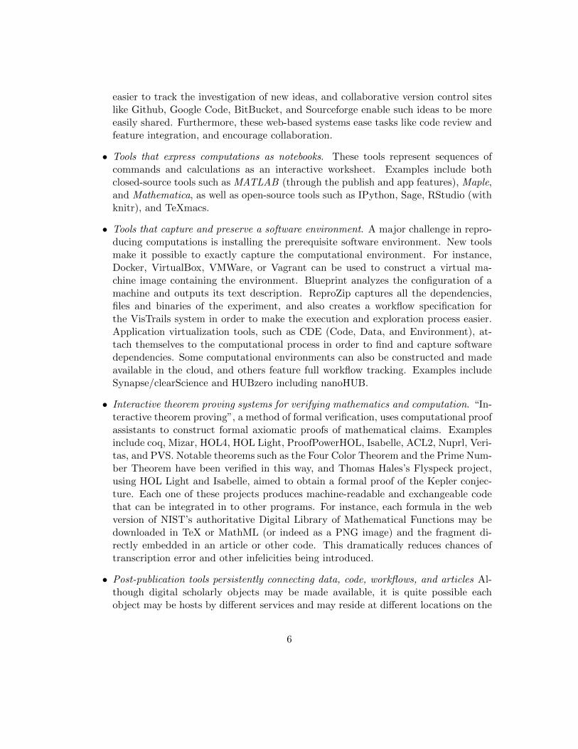
easier to track the investigation of new ideas, and collaborative version control siteslike Github, Google Code, BitBucket, and Sourceforge enable such ideas to be moreeasily shared. Furthermore, these web-based systems ease tasks like code review andfeature integration, and encourage collaboration.

• Tools that express computations as notebooks. These tools represent sequences ofcommands and calculations as an interactive worksheet. Examples include bothclosed-source tools such as MATLAB (through the publish and app features), Maple,and Mathematica, as well as open-source tools such as IPython, Sage, RStudio (withknitr), and TeXmacs.

• Tools that capture and preserve a software environment. A major challenge in repro-ducing computations is installing the prerequisite software environment. New toolsmake it possible to exactly capture the computational environment. For instance,Docker, VirtualBox, VMWare, or Vagrant can be used to construct a virtual ma-chine image containing the environment. Blueprint analyzes the configuration of amachine and outputs its text description. ReproZip captures all the dependencies,files and binaries of the experiment, and also creates a workflow specification forthe VisTrails system in order to make the execution and exploration process easier.Application virtualization tools, such as CDE (Code, Data, and Environment), at-tach themselves to the computational process in order to find and capture softwaredependencies. Some computational environments can also be constructed and madeavailable in the cloud, and others feature full workflow tracking. Examples includeSynapse/clearScience and HUBzero including nanoHUB.

• Interactive theorem proving systems for verifying mathematics and computation. “In-teractive theorem proving”, a method of formal verification, uses computational proofassistants to construct formal axiomatic proofs of mathematical claims. Examplesinclude coq, Mizar, HOL4, HOL Light, ProofPowerHOL, Isabelle, ACL2, Nuprl, Veri-tas, and PVS. Notable theorems such as the Four Color Theorem and the Prime Num-ber Theorem have been verified in this way, and Thomas Hales’s Flyspeck project,using HOL Light and Isabelle, aimed to obtain a formal proof of the Kepler conjec-ture. Each one of these projects produces machine-readable and exchangeable codethat can be integrated in to other programs. For instance, each formula in the webversion of NIST’s authoritative Digital Library of Mathematical Functions may bedownloaded in TeX or MathML (or indeed as a PNG image) and the fragment di-rectly embedded in an article or other code. This dramatically reduces chances oftranscription error and other infelicities being introduced.

• Post-publication tools persistently connecting data, code, workflows, and articles Al-though digital scholarly objects may be made available, it is quite possible eachobject may be hosts by different services and may reside at different locations on the

6

web (such as authors’ websites, journal supplemental materials documents, and var-ious data and code repositories). Services such as http://ResearchCompendia.org,http://RunMyCode.org and http://ipol.im attempt to co-locate these objects onthe web to enable both reproducibility and the persistent connection of these objects[52, 51].

The development of software tools enabling reproducible research is a new and rapidlygrowing area of research. We believe that the difficulty of working reproducibly will besignificantly reduced as these and other tools continue to be adopted and improved —and their use simplified. But prodding the scientific computing community, including re-searchers, funding agencies, journal editorial boards, lab mangers and promotion committeemembers, to broadly adopt and encourage such tools remains a challenge [41, 51].

2.3 Other cultural changes

While the above recommendations and tools will help, there is also a need to fundamentallyrethink the “reward system” in the scientific computing field (and indeed, of all scientificresearch that employs computing). Journal editors need to acknowledge importance ofcomputational details, and to encourage full documentation of the computational tech-niques, perhaps on an auxiliary persistent website if not in the journal itself. Reviewers,research institutions and, especially, funding agencies need to recognize the importance ofcomputing and computing professionals, and to allocate funding for after-the-grant supportand repositories. Also, researchers, journals and research institutions need to encouragepublication of negative results—other researchers can often learn from these experiences.Furthermore, as we have learned from other fields, only publishing “positive” results inad-vertently introduces a bias into the field.

3 Statistical overfitting

As mentioned above, the explosion of computing power and algorithms over the past fewdecades has placed computational tools of enormous power in the hands of practicing sci-entists. But one unfortunate side effect of this progress is that it has also greatly magnifiedthe potential for serious errors, such as statistical overfitting.

Statistical overfitting, in this context, means either proposing a model for an inputdataset that inherently possesses a higher level of complexity than that of the input datasetbeing used to generate or test it, or else trying many variations of a model on an inputdataset and then only presenting results from the one model variation that appears tobest fit the data. In many such cases, the model fits the data well only by fluke, sinceit is really fitting only the idiosyncrasies of the specific dataset in question, and has littleor no descriptive or predictive power beyond the particular dataset used in the analysis.

7

Statistical overfitting can be thought of as an instance of “selection bias,” wherein onepresents the results of only those tests that support well one’s hypothesis [34].

The problem of statistical overfitting in computational science is perhaps best illustratedin the field of mathematical finance. A frequently-encountered difficulty is that a proposedinvestment strategy or a fund based on this strategy looks great on paper, based on its“backtest” performance, but fall flat when actually fielded in practice.

In the field of finance, a backtest is the usage of a historical market dataset to test howa proposed investment strategy would have performed had it been in effect over the periodin question. The trouble is that in our present era, when a computer program can easilyanalyze thousands, millions or even billions of variations of a given investment strategy, itis almost certain that the optimal strategy, measured by its backtest performance, will bestatistically overfit and thus of dubious predictive value.

In two 2014 papers, two of the present authors (Bailey and Borwein, with two other col-laborators) derived formulas for (a) relating the number of trials to the minimum backtestlength, and (b) computing the probability of backtest overfitting. They also demonstratedthat under the assumption of memory in markets, overfit strategies are actually somewhatprone to lose money [13, 12].

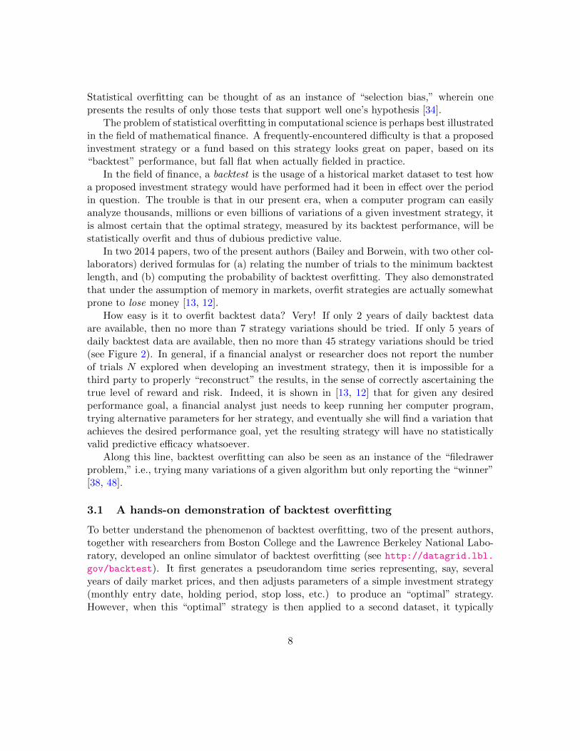
How easy is it to overfit backtest data? Very! If only 2 years of daily backtest dataare available, then no more than 7 strategy variations should be tried. If only 5 years ofdaily backtest data are available, then no more than 45 strategy variations should be tried(see Figure 2). In general, if a financial analyst or researcher does not report the numberof trials N explored when developing an investment strategy, then it is impossible for athird party to properly “reconstruct” the results, in the sense of correctly ascertaining thetrue level of reward and risk. Indeed, it is shown in [13, 12] that for given any desiredperformance goal, a financial analyst just needs to keep running her computer program,trying alternative parameters for her strategy, and eventually she will find a variation thatachieves the desired performance goal, yet the resulting strategy will have no statisticallyvalid predictive efficacy whatsoever.

Along this line, backtest overfitting can also be seen as an instance of the “filedrawerproblem,” i.e., trying many variations of a given algorithm but only reporting the “winner”[38, 48].

3.1 A hands-on demonstration of backtest overfitting

To better understand the phenomenon of backtest overfitting, two of the present authors,together with researchers from Boston College and the Lawrence Berkeley National Labo-ratory, developed an online simulator of backtest overfitting (see http://datagrid.lbl.

gov/backtest). It first generates a pseudorandom time series representing, say, severalyears of daily market prices, and then adjusts parameters of a simple investment strategy(monthly entry date, holding period, stop loss, etc.) to produce an “optimal” strategy.However, when this “optimal” strategy is then applied to a second dataset, it typically

8

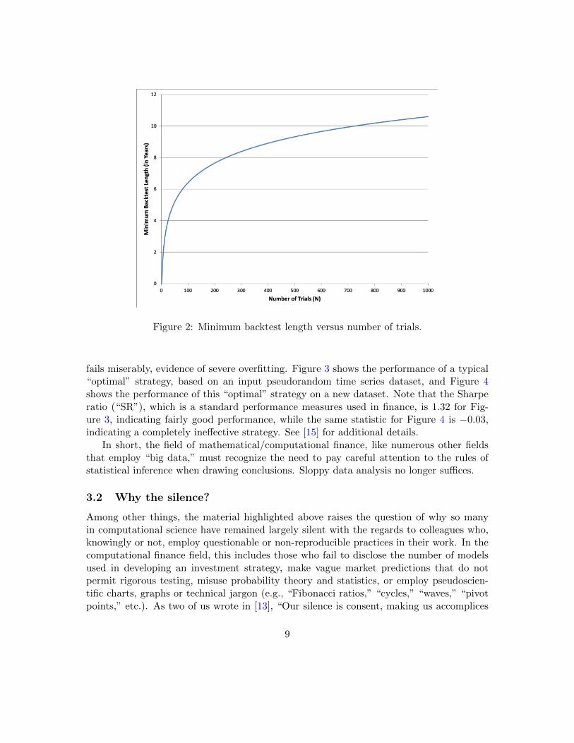
Figure 2: Minimum backtest length versus number of trials.

fails miserably, evidence of severe overfitting. Figure 3 shows the performance of a typical“optimal” strategy, based on an input pseudorandom time series dataset, and Figure 4shows the performance of this “optimal” strategy on a new dataset. Note that the Sharperatio (“SR”), which is a standard performance measures used in finance, is 1.32 for Fig-ure 3, indicating fairly good performance, while the same statistic for Figure 4 is −0.03,indicating a completely ineffective strategy. See [15] for additional details.

In short, the field of mathematical/computational finance, like numerous other fieldsthat employ “big data,” must recognize the need to pay careful attention to the rules ofstatistical inference when drawing conclusions. Sloppy data analysis no longer suffices.

3.2 Why the silence?

Among other things, the material highlighted above raises the question of why so manyin computational science have remained largely silent with the regards to colleagues who,knowingly or not, employ questionable or non-reproducible practices in their work. In thecomputational finance field, this includes those who fail to disclose the number of modelsused in developing an investment strategy, make vague market predictions that do notpermit rigorous testing, misuse probability theory and statistics, or employ pseudoscien-tific charts, graphs or technical jargon (e.g., “Fibonacci ratios,” “cycles,” “waves,” “pivotpoints,” etc.). As two of us wrote in [13], “Our silence is consent, making us accomplices

9

Figure 3: Final optimized strategy applied to input dataset. Note that the Sharpe ratio is1.32, indicating a fairly effective strategy on this dataset.

in these abuses.” And ignorance is a poor excuse.Similarly, in several instances when we have observed instances of reproducibility prob-

lems and sloppy data analysis within other arenas of scientific computing (see the next fewsections), a surprisingly typical reaction is to acknowledge that this is a significant problemin the field, but that it is either futile, unnecessary or inappropriate to make much fussabout it. Given recent experiences, it is clear that this approach is no longer acceptable.

4 Performance reporting in high-performance computing

One aspect of reproducibility in scientific computing that unfortunately is coming to thefore once again is the need for researchers to more carefully analyze and report data onthe performance of their codes.

10

Figure 4: Final optimized strategy applied to new dataset. Note that the Sharpe ratio is-0.03, indicating a completely ineffective strategy on this dataset.

4.1 A 1992 perspective

Some background is in order here. One of the present authors (Bailey) was privileged toparticipate in some of the earliest implementations and analysis of highly parallel scientificcomputing, back in the late 1980s and early 1990s. In this time period, many new parallelsystems had been introduced; each vendor claimed theirs was “best.” What’s more, manyscientific researchers were almost as excited about the potential of highly parallel systemsas were the computer vendors themselves. Few standard benchmarks and testing method-ologies had been established, so it was hard to reproduce published performance results.Thus much confusion reigned. Overall, the level of rigor and peer review in the field wasrelatively low.

In response, Bailey published a humorous essay entitled “Twelve ways to fool themasses,” which was intended to gently poke some fun at some of these less-than-rigorouspractices, hoping that this bit of humor would prod many in the community to tightentheir standards and be more careful when analyzing and reporting performance.

The “Twelve ways” article was published in Supercomputing Review, which subse-

11

quently went defunct. Here is a brief reprise, taken from [6]:

1. Quote 32-bit performance results, not 64-bit results, but don’t mention this in paper.

2. Present performance figures for an inner kernel, then represent these figures as theperformance of the entire application.

3. Quietly employ assembly code and other low-level language constructs.

4. Scale up the problem size with the number of processors, but omit any mention ofthis.

5. Quote performance results projected to a full system.

6. Compare your results against scalar, unoptimized code on conventional systems.

7. When run times are compared, compare with an old code on an obsolete system.

8. Base Mflop/s rates on the operation count of the parallel implementation, instead ofthe best practical serial algorithm.

9. Quote performance as processor utilization, parallel speedups or Mflop/s per dollar.

10. Mutilate the algorithm used in the parallel implementation to match the architecture.

11. Measure parallel run times on a dedicated system, but measure conventional runtimes in a busy environment.

12. If all else fails, show pretty pictures and animated videos, and don’t discuss perfor-mance.

Since abuses continued, Bailey subsequently published a paper in which he explicitlycalled out a number of these practices, citing actual examples from peer-reviewed papers(although the actual authors and titles of these papers were not presented in the paper,out of courtesy) [6]. Here is a brief summary of some of the examples:

• Scaling performance results to full-sized system. In some published papers and confer-ence presentations, performance results on small-sized parallel systems were linearlyscaled to full-sized systems, without even clearly disclosing this fact. For example,in several cases 8,192-CPU performance results were linearly scaled to 65,536-CPUresults, simply by multiplying by eight. Sometimes this fact came to light only inthe question-answer period of a technical presentation. A typical rationale was, “Wecan’t afford a full-sized system.”

12

• Using inefficient algorithms on highly parallel systems. In other cases, inefficientalgorithms were employed for the highly parallel implementation, requiring manymore operations, thus producing artificially high performance rates. For instance,some researchers cited partial differential equation simulation performance based ex-plicit schemes, for applications where implicit schemes were known to be much moreefficient. Another paper cited performance for computing a 3-D discrete Fouriertransform by direct evaluation of the defining formula, which requires 8n2 opera-tions, rather than by using a fast Fourier transform (FFT), which requires 5n log2 noperations. Obviously, for sufficiently large problems, FFT-based computations canproduce desired results with vastly fewer operations.

This is not to say that alternate algorithms should not be employed, but only thatwhen computing performance rates, one should base the operation count on the bestpractical serial algorithm, rather than on the actual number of operations performed(or cite both sets of figures).

• Not actually performing a claimed computation. One practice that was particularlytroubling was that of not actually performing computations that are mentioned inthe study. For example, in one paper the authors wrote in the Abstract that theirimplementation of a certain application on a CM-2 system (a parallel computer avail-able in the 1992 time frame) runs at “300-800 Mflop/s on a full [64K] CM-2, or atthe speed of a single processor of a Cray-2 on 1/4 of a CM-2.” However, in the actualtext of the paper, one reads that “This computation requires 568 iterations (taking272 seconds) on a 16K Connection Machine.” Note that it was actually run on 16,384processors, not 65,536 processors — the claimed performance figures in the Abstractevidently were merely the 16,384-CPU performance figures multiplied by four. Onethen reads that “In contrast, a Convex C210 requires 909 seconds to compute thisexample. Experience indicates that for a wide range of problems, a C210 is about 1/4the speed of a single processor Cray-2.” In other words, the authors did not actuallyperform the computation on a Cray-2, as clearly suggested in the Abstract; insteadthey ran the computation on a Convex C210 and employed a rather questionableconversion factor to obtain the Cray-2 figure.

• Questionable performance plots. The graphical representation of performance dataalso left much to be desired in many cases. Figure 5 shows a plot from one study thatcompares run times of various sizes of a certain computation on a parallel systems,in the lower curve, versus the same computations on a vector system (a widely usedscientific computer system at the time), in the upper curve. The raw data for thisgraph is as follows:

13

0

0.5

1

1.5

2

2.5

3

3.5

0 1000 2000 3000 4000 5000 6000 7000 8000 9000 10000

Number of Objects

Tim

e (H

ours

)

Figure 5: Performance plot [run time, parallel (lower) vs vector (upper)].

Problem size Parallel system Vector system(x axis) run time run time

20 8:18 0:1640 9:11 0:2680 11:59 0:57

160 15:07 2:11990 21:32 19:00

9600 31:36 3:11:50*

In the text of the paper where this plot appears, one reads that in the last entry,the 3:11:50 figure is an “estimate” — this problem size was not actually run on thevector system. The authors also acknowledged that the code for the vector systemwas not optimized for that system. Note however, by examining the raw data, thatthe parallel system is actually slower than the vector system for all cases, except forthe last (estimated) entry. Also, except for the last entry, all real data in the graphis in the lower left corner. In other words, the design of the plot leaves much to bedesired; a log-log plot should have been used for such data.

14

4.2 Fast forward to 2014: New ways to fool the masses

Perhaps given that a full generation has passed since the earlier era mentioned above,present-day researchers are not as fully aware of the potential pitfalls of performancereporting. In any event, various high-performance computing researchers have noted a“resurrection” of some of these questionable practices.

Even more importantly, the advent of many new computer architectures and designshas resulted in a number of “new” performance reporting practices uniquely suited to thesesystems. Here are some that are of particular concern:

• Citing performance rates for a run with only one processor core active in a shared-memory multi-core node, producing artificially inflated performance (since there is noshared memory interference) and wasting resources (since most cores are idle). Forexample, some studies have cited performance on “1024 cores” of a highly parallelcomputer system, even though the code was run on 1024 multicore nodes (each nodecontaining 16 cores), using only one core per node, and with 15 out of 16 cores idle oneach node. Note that since this implementation wastes 15/16 of the parallel systembeing used, it would never be tolerated in day-to-day usage.

• Claiming that since one is using a graphics processing unit (GPU) system, that effi-cient parallel algorithms must be discarded in favor of “more appropriate” algorithms.Again, while some algorithms may indeed need to be changed for GPU systems, itis important that when reporting performance, one base the operation count on thebest practical serial algorithm. See “Using inefficient algorithms on highly parallelsystems” in the previous subsection.

• Citing performance rates only for a core algorithm (such as FFT or linear systemsolution), even though full-scale applications have been run on the system (mostlikely because performance figures for the full-scale applications are not very good).

• Running a code numerous times, but only publishing the best performance figure inthe paper (recall the problems of the pharmaceutical industry from only publishingthe results of successful trials).

• Basing published performance results on runs using special hardware, operating sys-tem or compiler settings that are not appropriate for real-world production usage.

In each of these cases, note that in addition to issues of professional ethics and rigor,these practices result make it essentially impossible for other researchers to reconstructclaimed performance results, or to build on past research experiences to move the fieldforward. After all, if one set of researchers report that a given algorithm is the bestknown approach for performing a given application on a certain computer system, otherresearchers may also employ this approach, but then wonder why their performance resultsseem significantly less impressive than expected.

15

In other words, reproducible practices are more than just the “right” thing to do; theyare essential for making real progress in the field.

5 Numerical reproducibility

The ICERM report also emphasized rapidly growing challenge of numerical reproducibility:

Numerical round-off error and numerical differences are greatly magnified ascomputational simulations are scaled up to run on highly parallel systems.As a result, it is increasingly difficult to determine whether a code has beencorrectly ported to a new system, because computational results quickly divergefrom standard benchmark cases. And it is doubly difficult for other researchers,using independently written codes and distinct computer systems, to reproducepublished results [50].

5.1 Floating-point arithmetic

Difficulties with numerical reproducibility have their roots in the inescapable realities offloating-point arithmetic. “Floating-point arithmetic” means the common way of rep-resenting non-integer quantities on the computer, by means of a binary sign and expo-nent, followed by a binary mantissa — the binary equivalent of scientific notation, e.g.,3.14159 × 1013. For most combinations of operands, computer arithmetic operations in-volving floating-point numbers produce approximate results. Thus roundoff error is un-avoidable in floating-point computation.

For many scientific and engineering computations, particularly those involving empir-ical data, IEEE 32-bit floating-point arithmetic (roughly 7-digit accuracy) is sufficientlyaccurate to produce reliable, reproducible results, as required by the nature of the computa-tion. For more demanding applications, IEEE 64-bit arithmetic (roughly 15-digit accuracy)is required. Both formats are supported on almost all scientific computer systems.

Unfortunately, with the greatly expanded scale of computation now possible on theenormously powerful, highly parallel computer systems now being deployed, even IEEE64-bit arithmetic is sometimes insufficient. This is because numerical difficulties and sensi-tivities that are minor and inconsequential on a small-scale calculation may be major andhighly consequential once the computation is scaled up to petascale or exascale size. Insuch computations, numerical roundoff error may accumulate to the point that the courseof the computation is altered (i.e., by taking the wrong branch in a conditional branchinstruction), or else the final results are no longer reproducible across different computersystems and implementations, thus rendering the computations either useless or misleadingfor the science under investigation.

16

5.2 Numerical reproducibility problems in real applications

As a single example, the ATLAS (acronym for “A Toroidal LHC Apparatus”) experimentat the Large Hadron Collider must track charged particles to within 10-micron accuracyover a 10-meter run, and, with very high reliability, correctly identify them. The softwareportion of the experiment consists of over five million lines code (C++ and Python), whichhas been developed over many years by literally thousands of researchers.

Recently, some ATLAS researchers reported to us that in an attempt to improve per-formance of the code, they changed the underlying math library. When this was done,they found some collisions were missed and others were misidentified. That such a minorcode alteration (which should only affect the lowest-order bits produced by transcendentalfunction evaluations) had such a large high-level effect suggests that their code has signif-icant numerical sensitivities, and results may even be invalid in certain cases. How canthey possibly track down where these sensitivities occur, much less correct them?

As another example of this sort, researchers working with an atmospheric simulationcode had been annoyed by the difficulty of reproducing benchmark results. Even whentheir code was merely ported from one system to another, or run with a different numberof processors, the computed data typically diverged from a benchmark run after just a fewdays of simulated time. As a result, it was very difficult even for the developers of thiscode to ensure that bugs were not introduced into the code when changes are made, andeven more problematic for other researchers to reproduce their results. Some divergence isto be expected for computations of this sort, since atmospheric simulations are well-knownto be fundamentally “chaotic,” but did it really need to be so bad?

After an in-depth analysis of this code, researchers He and Ding found that merely byemploying double-double arithmetic (roughly 31-digit arithmetic) in two key summationloops, almost all of this numerical variability disappeared. With this minor change, bench-mark results could be accurately reproduced for a significantly longer time, with very littleincrease in run time [35].

Researchers working with some large computational physics applications reported sim-ilar difficulties with reproducibility. As with the atmospheric model code, they were ableto dramatically increase the reproducibility of their results by employing a form of customhigh-precision arithmetic in several critical summation loops [47].

5.3 High-precision arithmetic and numerical reproducibility

As noted above, using high-precision arithmetic (i.e., higher than the standard IEEE 64-bit arithmetic ) is often quite useful in ameliorating numerical difficulties and enhancingreproducibility.

By far the most common form of extra-precision arithmetic is known as “double-double”arithmetic (approximately 31-digit accuracy). This datatype consists of a pair of 64-bitIEEE floats (s, t), where s is the 64-bit floating-point value closest to the desired value, and

17

t is the difference (positive or negative) between the true value and s. “Quad-double” arith-metic operates on strings of four IEEE 64-bit floats, providing roughly 62-digit accuracy.Software to support these datatypes is widely available, e.g., the QD package [36].

Extensions of such schemes can be used to achieve any desired level of precision. Soft-ware to perform such computations has been available for quite some time, for example inthe commercial packages Mathematica and Maple. However, until 10 or 15 years ago thosewith applications written in more conventional languages, such as C++ or Fortran-90, of-ten found it necessary to rewrite their codes. Nowadays there are several freely availablehigh-precision software packages, together with accompanying high-level language inter-faces, utilizing operator overloading, that make code conversions relatively painless. Acurrent list of such software packages is given in [8].

Obviously there is an extra cost for performing high-precision arithmetic, but in manycases high-precision arithmetic is often only needed for a small portion of code, so that thetotal run time may increase only moderately.

Recently a team led by James Demmel of the University of California, Berkeley havebegun developing software facilities to find and ameliorate numerical anomalies in large-scale computations. These include facilities to: test the level of numerical accuracy requiredfor an application; delimit the portions of code that are inaccurate; search the space ofpossible code modifications; repair numerical difficulties, including usage of high-precisionarithmetic; and even navigate through a hierarchy of precision levels (32-bit, 64-bit orhigher) as needed. The current version of this tool is known as “Precimonious.” Detailsare presented in [49]. Some related research on numerical reproducibility is given in [44, 43].

5.4 Computations that require extra precision

While it may come as a surprise to some, there is a growing body of important scien-tific computations that actually requires high-precision arithmetic to obtain numericallyreliable, reproducible results. Typically such computations involve highly ill-conditionedlinear systems, large summations, long-time simulations, highly parallel simulations, high-resolution computations, or experimental mathematics computations.

The following example, condensed from [7], shows how the need for high-precisionarithmetic may arise even in very innocent-looking settings. Suppose one suspects that thedata (1, 32771, 262217, 885493, 2101313, 4111751, 7124761) are given by an integer polyno-mial for integer arguments (0, 1, . . . , 6). Most scientists and engineers will employ a familiarleast-squares scheme to recover this polynomial [46, pg. 44].

Performing these computations with IEEE 64-bit arithmetic and the LINPACK routines[1] for LU decomposition, with final results rounded to the nearest integer, finds the correctcoefficients (1, 0, 0, 32769, 0, 0, 1) (i.e., f(x) = 1 + (215 + 1)x3 + x6), but it fails when giventhe 9-long sequence generated by the function f(x) = 1 + (220 + 1)x4 + x8. On a MacProsystem, for example, the resulting rounded coefficients are (1, 6,−16, 14, 1048570, 2, 0, 0, 1),which differ badly from the correct coefficients (1, 0, 0, 0, 1048577, 0, 0, 0, 1).

18

From a numerical analysis point of view, a better approach is to employ a Lagrangeinterpolation scheme or the more sophisticated Demmel-Koev algorithm [25]. An imple-mentation of either scheme with 64-bit IEEE-754 arithmetic finds the correct polynomialin the degree-8 case, but even these schemes both fail in the degree-12 case. By contrast,merely by modifying a simple LINPACK program to employ double-double arithmetic,using the QD software [36], all three problems (degrees 6, 8 and 12) are correctly solvedwithout incident. See [7] for additional details.

There are numerous full-fledged scientific applications that also require higher precisionto obtain numerically reliable, reproducible results. Here is a very brief summary of someapplications that are known to the present authors. See [7] and [8] for additional details:

1. A computer-assisted solution of Smale’s 14th problem (18-digit arithmetic) [53].

2. Obtaining accurate eigenvalues for a class of anharmonic oscillators (18-digit arith-metic) [42].

3. Long-term simulations of the stability of the solar system [40, 29] (18-digit and 31-digit arithmetic).

4. Studies of n-body Coulomb atomic systems (120-digit arithmetic) [30].

5. Computing solutions to the Schrodinger equation (from quantum theory) for thelithium atom [56] and, using some of the same machinery, to compute a more accuratenumerical value of the fine structure constant of physics (approx. 7.2973525698×10−3)(31-digit arithmetic) [57].

6. Computing scattering amplitudes of collisions at the Large Hadron Collider (31-digitarithmetic) [28, 19, 45, 24].

7. Studies of dynamical systems using the Taylor method (up to 500-digit arithmetic)[16, 17, 18].

8. Studies of periodic orbits in dynamical systems using the Lindstedt-Poincare tech-nique of perturbation theory, together with Newton’s method for solving nonlinearsystems and Fourier interpolation (1000-digit arithmetic) [54, 55, 5].

6 High-precision arithmetic in experimental mathematicsand mathematical physics

Very high-precision floating-point arithmetic is essential to obtain reproducible results inexperimental mathematics and in related mathematical physics applications [20, 21]. In-deed, high-precision computation is now considered one of two staples of the field, alongwith symbolic computing (see the next section).

19

Many of these computations involve variants of Ferguson’s PSLQ integer relation detec-tion algorithm [14]. Given an n-long vector (xi) of floating-point numbers, the PSLQ algo-rithm finds the integer coefficients (ai), not all zero, such that a1x1 +a2x2 + · · ·+anxn = 0(to available precision), or else determines that there is no such relation within a certainbound on the size of the coefficients. Integer relation detection typically requires veryhigh precision, both in the input data and in the operation of the algorithm, to obtainnumerically reproducible results.

6.1 The BBP formula for π

One of the earliest applications of PSLQ and high-precision arithmetic was to numericallydiscover what is now known as the “BBP” formula for π:

π =

∞∑k=0

1

16k

(4

8k + 1− 2

8k + 4− 1

8k + 5− 1

8k + 6

).

This formula had not been known previously in the mathematical literature. It was dis-covered using computations with 200-digit arithmetic.

What is particularly remarkable about this formula is that after a simple manipulation,it can be used to calculate a string of binary or base-16 digits of π beginning at the n-thdigit, without needing to calculate any of the first n− 1 digits [20, pp. 135–143].

Since the discovery of the BBP formula in 1996, numerous other formulas of this typehave been found for other well-known mathematical constants, again by employing thePSLQ algorithm and very high-precision arithmetic. For example, two formulas of this typewere subsequently discovered for π2. One permits arbitrary-position digits to be calculatedin base 2 (binary), while the other permits arbitrary-position digits to be calculated in base3 (ternary).

6.2 Ising integrals

Very high-precision computations, combined with variants of the PSLQ algorithm, havebeen remarkably effective in mathematical physics settings. We summarize here just oneor two examples of this methodology in action, following [7] and some related referencesas shown below.

In one study, high-precision software was employed to study the following classes ofintegrals [10]. The Cn are connected to quantum field theory, the Dn integrals arise in the

20

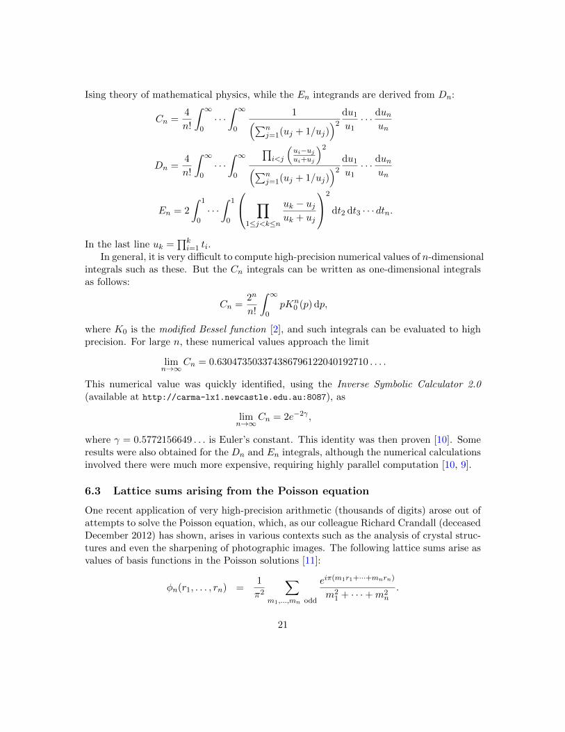
Ising theory of mathematical physics, while the En integrands are derived from Dn:

Cn =4

n!

∫ ∞0· · ·∫ ∞0

1(∑nj=1(uj + 1/uj)

)2 du1u1· · · dun

un

Dn =4

n!

∫ ∞0· · ·∫ ∞0

∏i<j

(ui−ujui+uj

)2(∑n

j=1(uj + 1/uj))2 du1

u1· · · dun

un

En = 2

∫ 1

0· · ·∫ 1

0

∏1≤j<k≤n

uk − ujuk + uj

2

dt2 dt3 · · · dtn.

In the last line uk =∏ki=1 ti.

In general, it is very difficult to compute high-precision numerical values of n-dimensionalintegrals such as these. But the Cn integrals can be written as one-dimensional integralsas follows:

Cn =2n

n!

∫ ∞0

pKn0 (p) dp,

where K0 is the modified Bessel function [2], and such integrals can be evaluated to highprecision. For large n, these numerical values approach the limit

limn→∞

Cn = 0.630473503374386796122040192710 . . . .

This numerical value was quickly identified, using the Inverse Symbolic Calculator 2.0(available at http://carma-lx1.newcastle.edu.au:8087), as

limn→∞

Cn = 2e−2γ ,

where γ = 0.5772156649 . . . is Euler’s constant. This identity was then proven [10]. Someresults were also obtained for the Dn and En integrals, although the numerical calculationsinvolved there were much more expensive, requiring highly parallel computation [10, 9].

6.3 Lattice sums arising from the Poisson equation

One recent application of very high-precision arithmetic (thousands of digits) arose out ofattempts to solve the Poisson equation, which, as our colleague Richard Crandall (deceasedDecember 2012) has shown, arises in various contexts such as the analysis of crystal struc-tures and even the sharpening of photographic images. The following lattice sums arise asvalues of basis functions in the Poisson solutions [11]:

φn(r1, . . . , rn) =1

π2

∑m1,...,mn odd

eiπ(m1r1+···+mnrn)

m21 + · · ·+m2

n

.

21

k Minimal polynomial for exp(8πφ2(1/k, 1/k))

5 1 + 52α− 26α2 − 12α3 + α4

6 1− 28α+ 6α2 − 28α3 + α4

7 −1− 196α+ 1302α2 − 14756α3 + 15673α4

+42168α5 − 111916α6 + 82264α7 − 35231α8

+19852α9 − 2954α10 − 308α11 + 7α12

8 1− 88α+ 92α2 − 872α3 + 1990α4 − 872α5

+92α6 − 88α7 + α8

9 −1− 534α+ 10923α2 − 342864α3 + 2304684α4

−7820712α5 + 13729068α6

−22321584α7 + 39775986α8 − 44431044α9

+19899882α10 + 3546576α11

−8458020α12 + 4009176α13 − 273348α14

+121392α15 − 11385α16 − 342α17 + 3α18

10 1− 216α+ 860α2 − 744α3 + 454α4 − 744α5

+860α6 − 216α7 + α8

Table 1: Minimal polynomials discovered by very high precision PSLQ computations.

By noting some striking connections with Jacobi theta-function values, Crandall, Zucker,and two of the present authors were are able to develop new closed forms for certainvalues of the arguments rk [11]. In particular, after extensive high-precision numericalexperimentation, they discovered, then were able to prove, the remarkable fact that forrational numbers x and y,

φ2(x, y) =1

πlogA, (1)

where A is an algebraic number, namely the root of an algebraic equation with integercoefficients.

In this case they computed α = A8 = exp(8πφ2(x, y)) (as it turned out, the ‘8’ substan-tially reduces the degree of polynomials and so computational cost), and then generatedthe vector (1, α, α2, · · · , αd), which, for various conjectured values of d, was input to amultipair PSLQ program. When successful, the PSLQ program returned the vector ofinteger coefficients (a0, a1, a2, · · · , ad) of a polynomial satisfied by α as output. With someexperimentation on the degree d, and after symbolic verification using Mathematica, theywere able to ensure that the resulting polynomial is in fact the minimal polynomial sat-isfied by α. Table 1 shows some examples of the minimal polynomials discovered by thisprocess. Using this data, they were able to conjecture a formula that gives the degree d asa function of k [11].

These computations required prodigiously high precision to produce reproducible re-

22

sults: up to 20,000-digit floating-point arithmetic in some cases, such as in finding thedegree-128 polynomial satisfied by α = exp(8πφ2(1/32, 1/32)). Related computations in afollow-up study required up to 50,000-digit arithmetic.

In each of these examples, the usage of very high-precision arithmetic is not optional,but absolutely essential to the computation — the relations in question could not possi-bly be recovered in a reliable, reproducible fashion except by using these exalted levels ofprecision. Future research in this field will focus not only on how to perform such com-putations in the most efficient way possible, but also how to explore and then certify thatthe precision level used in such computations is sufficient to obtain reproducible results.

7 Reproducibility in symbolic computing

Closely related to the high-precision computations described in the past two sections is theusage of symbolic computing in experimental mathematics and mathematical physics. Atthe present time, the commercial packages Maple and Mathematica are most commonlyused for symbolic computations, although other packages, such as Sage and Magma arealso used by some.

But like all other classes of computer software, symbolic manipulation software hasbugs and limitations. In some cases, the software itself detects that it has encountereddifficulties, and outputs messages acknowledging that its results might not be reliable. Butnot always.

For example, consider the integral

W2 =

∫ 1

0

∫ 1

0

∣∣e2πix + e2πiy∣∣ dx dy, (2)

which arose in research into the properties of n-step random walks on the plane [23, 39].The latest editions of Maple (version 18) and Mathematica (version 9) both declare thatW2 = 0, in spite of the obvious fact that this integral is positive and nonzero. IndeedW2 = 4/π is the expected distance traveled by a uniform random walk in two steps. It isworth pointing out that (2) can easily be rewritten as

W2 =

∫ 1

0|e2πix|

(∫ 1

0|1 + e2πi(y−x)|dy

)dx =

∫ 1

0|1 + e2πiy| dy, (3)

which is in a form that both Maple and Mathematica can evaluate, but this “human”observation is not exploited by the commercial packages. Whether this behavior is a “bug”or a “feature” is matter of some dispute, although it is fair to expect the package to notifythe user that the integrand function is problematic.

As another example, three researchers in Spain encountered difficulties with Mathemat-ica while attempting to check a number theory conjecture. They ultimately found errorsthat they could exhibit even in fairly modest-sized examples. For example, they presented

23

an example involving a 14 × 14 matrix of pseudorandom integers between −99 and 99,which was then multiplied by a certain diagonal matrix with large entries, and then addedto another matrix of pseudorandom integers between −999 and 999. When they thenattempted to compute the determinant of the resulting fixed matrix using Mathematicaversion 9, the found that the results were not consistent — they often obtained differentanswers for the same problem [27]. This problem now seems to have been resolved inMathematica version 10, according to some tests by the present authors.

Symbolic computing applications often are quite expensive, with jobs running for manyhours, days or months. For example, recently three researchers attempted to update anearlier effort to explore Giuga’s 1950 conjecture, which is that an integer n ≥ 2 is prime ifand only if

n−1∑k=1

kn−1 ≡ −1 (mod n). (4)

They computationally verified this conjecture for all composite n with up to 4771 primefactors, which means that any counterexample must have at least 19,907 digits. Thismultithreaded computation required 95 hours. Increasing this bound significantly wouldcurrently take decades or centuries [22].

8 Why should we trust the results of computation?

These examples raise the question of why should anyone trust the results of any com-putation, numeric or symbolic. After all, there are numerous potential sources of error,including user programming bugs, symbolic software bugs, compiler bugs, hardware errors,and I/O errors. None of these can be categorically ruled out. However, substantial confi-dence can be gained in a result by reproducing it with different software systems, hardwaresystems, programming systems, or by repeating the computation with detailed checks ofintermediate results.

For example, programmers of large computations of digits of π have for many years cer-tified their results by repeating the computation using a completely different algorithm. Ifall but a few trailing digits agree, then this is impressive evidence that both computationsare almost certainly correct. In a similar vein, programmers of large, highly parallel nu-merical simulations, after being warned by systems administrators that occasional systemhardware or software errors are inevitable, are inserting internal checks into their codes. Forexample, in problems where the computation carries forward both a large matrix and itsinverse, programmers have inserted periodic checks that the product of these two matricesis indeed the identity matrix, to within acceptable numerical error.

In other cases, researchers are resorting to formal methods, wherein results are verifiedby software that performs a computer verification of every logical inference in the proof,back to the fundamental axioms of mathematics. For example, University of Pittsburgh

24

researcher Thomas Hales recently completed a computer-aided proof of the Kepler conjec-ture, namely the assertion that the most efficient way to pack equal-sized spheres is thesame scheme used by grocers to stack oranges [31]. Some objected to this approach, soHales has attempted to re-do the proof using formal methods [32]. This project is nowcomplete [33].

8.1 Is “Free” Software Better?

We conclude by briefly commenting on open-source versus commercial software (a fulltreatment would require discussion of complexities such as licensing, user adoption, andnumerous other topics). Some open-source software for mathematical computing is quitepopular. For example, GeoGebra, which is based on Cabri, is now very popular in schoolsas replacement for Sketchpad. But the question is whether such software will be preservedwhen the core group of founders and developers lose interest or move on to other projectsor employment. This is also an issue with large-scale commercial products, but it is morepronounced with open-source project.

One advantage of Maple over Mathematica is that most of the Maple source code isaccessible, while Mathematica is entirely sealed. As a result, it is often difficult to trackdown or rectify problems that arise. Similarly, Cinderella is very robust, unlike GeoGebra,and mathematically sophisticated—using Riemann surfaces to ensure that complicatedconstructions do not crash. That said, it is the product of two talented and committedmathematicians but only two, and it is only slightly commercial. In general, softwarevendors and open source producers do not provide the teacher support that has is assumedin the textbook market.

One other word of warning is given by the experience of the Heartbleed bug [3], whichmany cybersecurity observers termed “catastrophic.” This is a bug in the OpenSSL cryp-tography library, which is incorporated in many other software packages, commercial andopen-source. A fixed version of the OpenSSL was quickly released, but it will take time toidentify all instances. In this case, although almost everyone uses the flawed software, noone really “owns” it, making ongoing maintenance problematic.

9 Conclusions

The advent of high-performance computer systems, all the way from laptops and worksta-tions to systems with thousands or even millions of processing elements, has opened newvistas to the field of scientific computing and computer modeling. It has revolutionized nu-merous fields of scientific research, from climate modeling and materials science to proteinbiology, nuclear physics and even research mathematics (as we have seen in the examplesabove). In the coming years, this technology will be exploited in numerous industrial andengineering applications as well, including “virtual” product testing and market analysis.

25

However, like numerous other fields that are embracing “big data,” scientific computingmust confront issues of reliability and reproducibility, both in computed results and alsoin auxiliary statistical analysis, visualization and performance. For one thing, these com-putations are becoming very expensive, both in terms of the acquisition and maintenancecosts of the supercomputers being used, but even more so in terms of the human time todevelop and update the requisite application programs.

Thus it is increasingly essential that reliability and reproducibility be foremost in theseactivities: designing the workflow process right from the start to ensure reliability and re-producibility — carefully documenting each step, including code preparation, data prepa-ration, execution, post-execution analysis and visualization, through to the eventual publi-cation of the results. A little effort spent early on will be rewarded with much less confusionand much more productivity at the end.

References

[1] Linpack. Available at http://www.netlib.org/linpack.

[2] NIST digital library of mathematical functions. Available at http://dlmf.nist.gov.

[3] Heartbleed. 2014. Available at http://en.wikipedia.org/wiki/Heartbleed.

[4] Top500 list. July 2014. Available at http://top500.org/statistics/perfdevel.

[5] A. Abad, R. Barrio, and A. Dena. Computing periodic orbits with arbitrary precision.Phys. Rev. E, 84:016701, 2011.

[6] D. H. Bailey. Misleading performance reporting in the supercomputing field. ScientificProgramming, 1:141–151, 1992.

[7] D. H. Bailey, R. Barrio, and J. M. Borwein. High-precision computation: Mathemat-ical physics and dynamics. Appl. Math. and Computation, 218:10106–10121, 2012.

[8] D. H. Bailey and J. M. Borwein. High-precision arithmetic: Progress and challenges.Available at http://www.davidhbailey.com/dhbpapers/hp-arith.pdf.

[9] D. H. Bailey and J. M. Borwein. Hand-to-hand combat with thousand-digit integrals.J. of Computational Science, 3:77–86, 2012.

[10] D. H. Bailey, J. M. Borwein, and R. E. Crandall. Integrals of the Ising class. J. PhysicsA: Math. and Gen., 39:12271–12302, 2006.

[11] D. H. Bailey, J. M. Borwein, R. E. Crandall, and J. Zucker. Lattice sums arising fromthe Poisson equation. J. Physics A: Math. and Theor., 46:115201, 2013.

26

[12] D. H. Bailey, J. M. Borwein, M. Lopez de Prado, and Q. J. Zhu. The probability ofbacktest overfitting. Available at http://ssrn.com/abstract=2326253.

[13] D. H. Bailey, J. M. Borwein, M. Lopez de Prado, and Q. J. Zhu. Pseudo-mathematicsand financial charlatanism: The effects of backtest overfitting on out-of-sample per-formance. Notices of the American Mathematical Society, pages 458–471, May 2014.

[14] D. H. Bailey and D. Broadhurst. Parallel integer relation detection: Techniques andapplications. Math. of Computation, 70:1719–1736, 2000.

[15] D. H. Bailey, S. Ger, M. Lopez de Prado, A. Sim, and K. Wu. Statistical overfit-ting and backtest performance. 2014. Available at http://www.davidhbailey.com/

dhbpapers/overfitting.pdf.

[16] R. Barrio. Performance of the Taylor series method for ODEs/DAEs. Appl. Math.Comput., 163:525–545, 2005.

[17] R. Barrio. Sensitivity analysis of odes/daes using the Taylor series method. SIAM J.Sci. Computing, 27:1929–1947, 2006.

[18] R. Barrio, F. Blesa, and M. Lara. VSVO formulation of the Taylor method for thenumerical solution of ODEs. Comput. Math. Appl., 50:93–111, 2005.

[19] C. F. Berger, Z. Bern, L. J. Dixon, F. F. Cordero, D. Forde, H. Ita, D. A. Kosower, andD. Maitre. An automated implementation of on-shell methods for one-loop amplitudes.Phys. Rev. D, 78, 2008.

[20] J. M. Borwein and D. H. Bailey. Mathematics by Experiment: Plausible Reasoning inthe 21st Century. A.K. Peters, Natick, MA, second edition, 2008.

[21] J. M. Borwein, D. H. Bailey, and R. Girgensohn. Experimentation in Mathematics:Computational Paths to Discovery. A.K. Peters, Natick, MA, 2004.

[22] J. M. Borwein, M. Skerritt, and C. Maitland. Computation of a lower bound to Giuga’sprimality conjecture. Integers, 13, 2013. Available at http://www.carma.newcastle.edu.au/jon/giuga2013.pdf.

[23] J. M. Borwein and A. Straub. Mahler measures, short walks and logsine integrals.Theoretical Computer Science. Special issue on Symbolic and Numeric Computation,479:4–21, 2013. DOI: http://link.springer.com/article/10.1016/j.tcs.2012.10.025.

[24] M. Czakon. Tops from light quarks: Full mass dependence at two-loops in QCD. Phys.Lett. B, 664:307, 2008.

27

[25] J. Demmel and P. Koev. The accurate and efficient solution of a totally positivegeneralized vandermonde linear system. SIAM J. of Matrix Analysis Appl., 27:145–152, 2005.

[26] D. Donoho, A. Maleki, M. Shahram, V. Stodden, and I. U. Rahman. Reproducibleresearch in computational harmonic analysis. Computing in Science and Engineering,11, January 2009.

[27] A. J. Duran, M. Perez, and J. L. Varona. Misfortunes of a mathematicians’ trio usingcomputer algebra systems: Can we trust? 2014. Available at http://arxiv.org/

abs/1312.3270.

[28] R. K. Ellis, W. T. Giele, Z. Kunszt, K. Melnikov, and G. Zanderighi. One-loopamplitudes for w+ 3 jet production in hadron collisions. Available at http://arXiv.org/abs/0810.2762.

[29] A. Farres, J. Lsaskar, S. Blanes, F. Casas, J. Makazaga, and A. Murua. High preci-sion symplectic integrators for the solar system. Celestial Mechanics and DynamicalAstronomy, 116:141–174, 2013.

[30] A. M. Frolov and D. H. Bailey. Highly accurate evaluation of the few-body auxiliaryfunctions and four-body integrals. J. Physics B, 36:1857–1867, 2003.

[31] T. C. Hales. A proof of the kepler conjecture. Annals of Mathematics, 162:10651185,2005.

[32] T. C. Hales. Lessons learned from the flyspeck project. 2011. Avail-able at http://www-sop.inria.fr/manifestations/MapSpringSchool/contents/

ThomasHales.pdf.

[33] T. C. Hales. The flyspeck project. 2014. Available at https://code.google.com/p/flyspeck/wiki/AnnouncingCompletion.

[34] D. J. Hand. The Improbability Principle. Macmillan, New York, 2014.

[35] Y. He and C. Ding. Using accurate arithmetics to improve numerical reproducibilityand stability in parallel applications. J. Supercomputing, 18:259–277, 2001.

[36] Y. Hida, X. S. Li, and D. H. Bailey. Algorithms for quad-double precision floatingpoint arithmetic. Proc. of the 15th IEEE Symposium on Computer Arithmetic, 2001.

[37] J. Ioannidis. Why most published research findings are false. PLoS Med, 2(8), 2005.

[38] J. P. A. Ioannidis. Why most published research findings are false. PLOS Medicine,August 2005. DOI: 10.1371/journal.pmed.0020124.

28

[39] M. S. J. M. Borwein and C. Maitland. Computation of a lower bound to Giuga’sprimality conjecture. Proceedings of Integers13, 2013. Available at http://www.

westga.edu/~integers/cgi-bin/get.cgi.

[40] G. Lake, T. Quinn, and D. C. Richardson. From Sir Isaac to the Sloan survey:Calculating the structure and chaos due to gravity in the universe. Proc. of the 8thACM-SIAM Symposium on Discrete Algorithms, pages 1–10, 1997.

[41] R. LeVeque, I. Mitchell, and V. Stodden. Reproducible research for scientific com-puting: Tools and strategies for changing the culture. Computing in Science andEngineering, pages 13–17, July 2012.

[42] M. H. Macfarlane. A high-precision study of anharmonic-oscillator spectra. Annals ofPhysics, 271:159–202, 1999.

[43] H. D. Nguyen and J. Demmel. Fast reproducible floating point summation. In Pro-ceedings of the 21st IEEE Symposium on Computer Arithmetic, 2013.

[44] H. D. Nguyen and J. Demmel. Numerical accuracy and reproducibility at exascale.In Proceedings of the 21st IEEE Symposium on Computer Arithmetic, 2013.

[45] G. Ossola, C. G. Papadopoulos, and R. Pittau. Cuttools: A program implementingthe OPP reduction method to compute one-loop amplitudes. J. High-Energy Phys.,0803:04, 2008.

[46] W. H. Press, S. A. Eukolsky, W. T. Vetterling, and B. P. Flannery. Numerical Recipes:The Art of Scientific Computing. Cambridge University Press, 3 edition, 2007.

[47] R. W. Robey, J. M. Robey, and R. Aulwes. In search of numerical consistency inparallel programming. Parallel Computing, 37:217–219, 2011.

[48] J. P. Romano and M. Wolf. Stepwise multiple testing as formalized data snooping.Econometrica, pages 1237–1282, July 2005.

[49] C. Rubio-Gonzalez, C. Nguyen, H. D. Nguyen, J. Demmel, W. Kahan, K. Sen, D. H.Bailey, and C. Iancu. Precimonious: Tuning assistant for floating-point precision. Proc.of SC13. Available at http://www.davidhbailey.com/dhbpapers/precimonious.

pdf.

[50] V. Stodden, D. H. Bailey, J. M. Borwein, R. J. LeVeque, W. Rider, and W. Stein.Setting the default to reproducible: Reproducibility in computational and exper-imental mathematics. Available at http://www.davidhbailey.com/dhbpapers/

icerm-report.pdf.

29

[51] V. Stodden, S. Miguez, and J. Seiler. Researchcompendia.org: Cyberinfrastructurefor reproducibility and collaboration in computational science. Computing in Scienceand Engineering, 2014, to appear.

[52] V. Stodden, S. Miguez, and J. Seiler. Researchcompendia: Cyberinfrastructure forreproducibility and collaboration in computational science. Computing in Science andEngineering, January 2015.

[53] W. Tucker. Smale’s 14th problem. Foundations of Computational Mathematics, 2:53–117, 2002.

[54] D. Viswanath. The fractal property of the Lorenz attractor. J. Phys. D, 190:115–128,2004.

[55] D. Viswanath and S. Sahutoglu. Complex singularities and the Lorenz attractor. SIAMReview, 52:294–314, 2010.

[56] Z.-C. Yan and G. W. F. Drake. Bethe logarithm and QED shift for Lithium. Phys.Rev. Letters, 81:774–777, 2003.

[57] T. Zhang, Z.-C. Yan, and G. W. F. Drake. QED corrections of O(mc2α7 lnα) to thefine structure splittings of Helium and He-like ions. Physical Review Letters, 77:1715–1718, 1994.

30