satellite and radar survey of mesoscale …rams.atmos.colostate.edu/cotton/vita/141.pdf2428 monthly...

2428 VOLUME 131M O N T H L Y W E A T H E R R E V I E W

q 2003 American Meteorological Society

Satellite and Radar Survey of Mesoscale Convective System Development

ISRAEL L. JIRAK, WILLIAM R. COTTON, AND RAY L. MCANELLY

Colorado State University, Fort Collins, Colorado

(Manuscript received 14 November 2002, in final form 7 April 2003)

ABSTRACT

An investigation of several hundred mesoscale convective systems (MCSs) during the warm seasons (April–August) of 1996–98 is presented. Circular and elongated MCSs on both the large and small scales were classifiedand analyzed in this study using satellite and radar data. The satellite classification scheme used for this studyincludes two previously defined categories and two new categories: mesoscale convective complexes (MCCs),persistent elongated convective systems (PECSs), meso-b circular convective systems (MbCCSs), and meso-belongated convective systems (MbECSs). Around two-thirds of the MCSs in the study fell into the larger satellite-defined categories (MCCs and PECSs). These larger systems produced more severe weather, generated muchmore precipitation, and reached a peak frequency earlier in the convective season than the smaller, meso-bsystems. Overall, PECSs were found to be the dominant satellite-defined MCS, as they were the largest, mostcommon, most severe, and most prolific precipitation-producing systems.

In addition, 2-km national composite radar reflectivity data were used to analyze the development of each ofthe systems. A three-level radar classification scheme describing MCS development is introduced. The classi-fication scheme is based on the following elements: presence of stratiform precipitation, arrangement of con-vective cells, and interaction of convective clusters. Considerable differences were found among the systemswhen categorized by these features. Grouping systems by the interaction of their convective clusters revealedthat more than 70% of the MCSs evolved from the merger of multiple convective clusters, which resulted inlarger systems than those that developed from a single cluster. The most significant difference occurred whenclassifying systems by their arrangement of convective cells. In particular, if the initial convection were linearlyarranged, the mature MCSs were larger, longer-lived, more severe, and more effective at producing precipitationthan MCSs that developed from areally arranged convection.

1. Introduction

Mesoscale convective systems (MCSs) are significantrain-producing weather systems for the central UnitedStates during the warm season (Fritsch et al. 1986).Additionally, MCSs produce a broad range of severeconvective weather events (Maddox et al. 1982; Houzeet al. 1990) that are potentially damaging and dangerousto society in general. Given the profound influence thatMCSs have on the midlatitudes, continued study is es-sential in gaining a deeper insight of these systems.

Even though the importance of MCSs is well under-stood, there is much left to learn about the growth anddevelopment of these systems. One approach that hasbeen used to study MCSs involves classifying the sys-tems and analyzing the differences among the catego-ries. For example, infrared satellite imagery has beenan important means of studying a particular type of MCScalled the mesoscale convective complex (e.g., Maddox1980, 1983; Maddox et al. 1982; McAnelly and Cotton

Corresponding author address: Israel L. Jirak, Department of At-mospheric Science, Colorado State University, Fort Collins, CO80523.E-mail: [email protected]

1986; Cotton et al. 1989). Although satellite imagesprovide an effective way of identifying MCSs, they donot provide much information on the underlying con-vection. Consequently, radar data have been used toallow for more detailed classification studies of MCSconvection (e.g., Bluestein and Jain 1985; Bluestein etal. 1987; Houze et al. 1990; Parker and Johnson 2000).

While both satellite and radar data have been usedindependently to study samples of MCSs, there have notbeen any large, detailed MCS inquiries using both typesof data. Additionally, previous studies have generallyfocused on a particular type of MCS, but this studyexamines circular and elongated systems on both thelarge and small scales. The purpose of this investigationis to supplement prior studies on MCS classification byproviding a more comprehensive satellite and radar sur-vey of MCSs in terms of number of systems, type ofsystems, length of study, and geographical area consid-ered. The focus of the classification scheme is directedtoward the developmental stages to better characterizecommon patterns by which convection becomes orga-nized into mature MCSs.

Relevant observational MCS studies done in the pastare discussed and related to the present study in section

OCTOBER 2003 2429J I R A K E T A L .

TABLE 1. Modified mesoscale convective complex(MCC) definition.

Physical characteristics

Size Cloud shield with continuously low IRtemperature #2528C must have an area$50 000 km2.

Initiate Size definition is first satisfied.Duration Size definition must be met for a period

$6 h.Maximum extent Contiguous cold cloud shield (IR tempera-

ture #2528C) reaches a maximum size.Shape Eccentricity (minor axis/major axis) $0.7

at time of maximum extent.Terminate Size definition no longer satisfied.

TABLE 2. MCS definitions based upon analysis of IR satellite data.

MCS category Size Duration Shape

MCC Cold cloud region # 2528C witharea $ 50 000 km2

Size definition met for$6 h

Eccentricity $ 0.7 at time of maxi-mum extent

PECS 0.2 # Eccentricity , 0.7 at time ofmaximum extent

MbCCS Cold cloud region # 2528C witharea $ 30 000 km2 and maxi-mum size must be $50 000 km2

Size definition met for$3 h

Eccentricity $ 0.7 at time of maxi-mum extent

MbECS 0.2 # Eccentricity , 0.7 at time ofmaximum extent

2. Section 3 provides an overview of the data and meth-ods used in this analysis. The infrared satellite classi-fications are defined and discussed in section 4 withsome basic comparisons. Section 5 discusses the methodused to categorize the development of MCSs as seen byradar imagery. In addition, this section provides someexamples and basic characteristics of each category.Further analysis of the environment, severe weather, andlife cycles of each MCS category is provided in section6. Finally, section 7 provides a summary and conclu-sions.

2. Background

Several MCS studies performed in the past have at-tempted to classify MCSs into discrete categories by avariety of different methods and perspectives. The mostcommon methods of MCS classification have involvedanalyzing satellite and radar characteristics of the sys-tems. Similar to past studies, the present study attemptsto classify MCSs to better understand the similaritiesand differences between the systems; however, unlikepast studies, this study will classify each MCS by bothsatellite and radar characteristics. Several studies on theclassification of MCSs by satellite and radar character-istics have emerged in the past 20 yr, and the mostinfluential studies are discussed in the following sub-sections.

a. Satellite classification of MCSs

Maddox (1980) first classified a particular type ofMCS by means of satellite imagery. He noticed a highfrequency of organized, quasi-circular, meso-a (see Or-lanski 1975) convective weather systems moving acrossthe central United States. He termed these massive sys-tems mesoscale convective complexes (MCCs). Hebased the definition of MCCs on typical infrared satellitecharacteristics possessed by systems moving across thecentral United States. The only minor modification thathas been made to Maddox’s original definition of MCCswas by Augustine and Howard (1988) to remove the#2328C size requirement of the cloud shield in orderto simplify the identification and documentation pro-cedure of MCCs. This modified MCC definition isshown in Table 1 and is used in the current study. It isnoteworthy to mention that Cotton et al. (1989) set forthan alternative dynamical definition of MCCs, which re-lates the horizontal scale of MCCs to the Rossby radiusof deformation. Another large class of MCSs, persistentelongated convective systems (PECS), was identified ina study by Anderson and Arritt (1998). PECS are whatmight be considered the ‘‘linear’’ version of MCCs, asthe only difference between a MCC and a PECS is theshape of the system (Table 2). PECSs have eccentricitiesbetween 0.2 and 0.7 while MCCs must have eccentric-ities $0.7. The definitions of MCCs and PECSs will beused along with two other definitions to include smallerMCSs in a satellite classification scheme for this study.

b. Radar classification of MCSs

Unlike the relatively objective satellite classificationprocess, the radar classification process is much moresubjective. Two basic methods of categorizing MCSsby radar characteristics have evolved over time. Onecommon method has been to examine the arrangementof the convective and stratiform regions of a matureMCS, including classifications such as leading-line/trailing stratiform (TS), parallel stratiform (PS), andleading stratiform (LS) MCSs (e.g., Houze et al. 1990;Parker and Johnson 2000). Another common, yet dif-ferent, method of MCS radar classification has been toclassify MCSs based on their developmental or for-


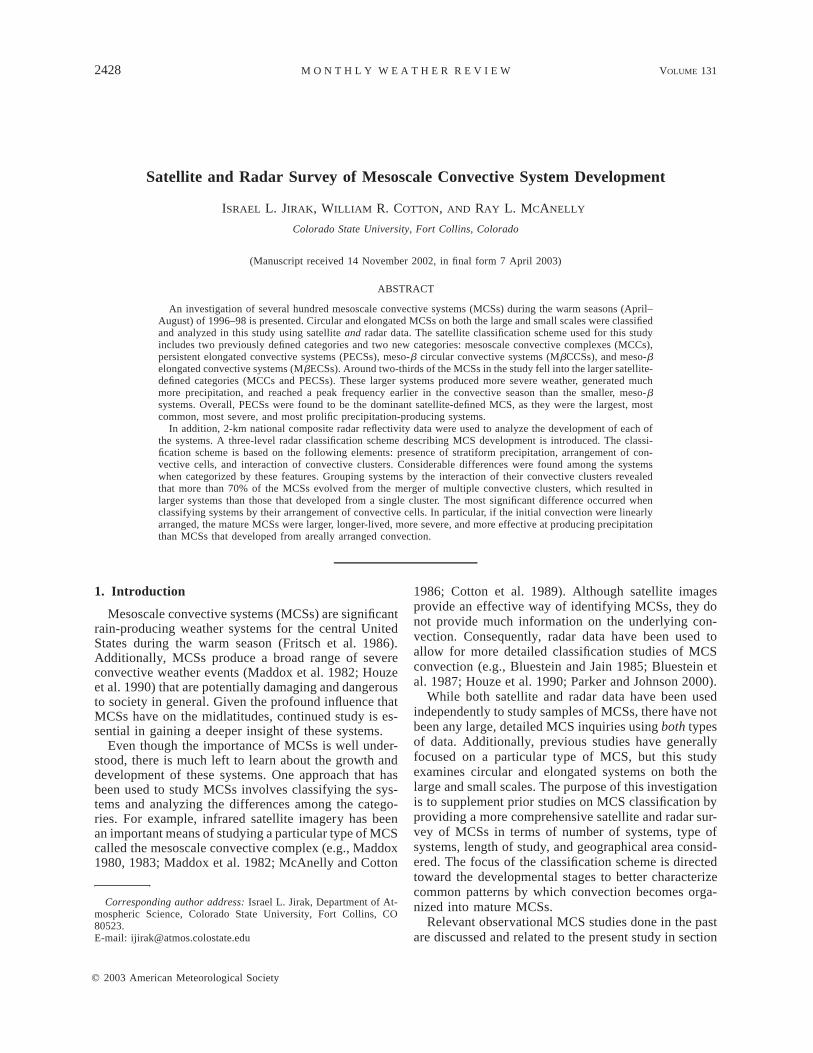
FIG. 1. Idealized depictions of squall-line formation (fromBluestein and Jain 1985).

mative stages (e.g., Bluestein and Jain 1985; Bluesteinet al. 1987; Blanchard 1990; Loehrer and Johnson1995). As previously mentioned, the focus of this studylies in the development of MCSs, so only those studiesrelating to this topic will be discussed further.

Bluestein and Jain (1985) performed the first studyof this type seeking to identify common patterns of se-vere squall-line formation. They considered the generaldefinition of squall line (i.e., ‘‘a linearly oriented me-soscale convective system’’) in their examination of datafrom a single-radar site over central Oklahoma. Squall-line development was divided into four classifications:broken line, back building, broken areal, and embeddedareal (see Fig. 1). The broken-line and back-buildingcategories were the most common type of formation andwere the easiest to distinguish using satellite imagery.However, they made no attempt beyond this to observeand classify squall lines by satellite characteristics. Ina closely related study, Bluestein et al. (1987) studiedthe formation of nonsevere squall lines in Oklahomaand found that the broken-areal category was the mostcommon type of formation for nonsevere squall lines.

Other studies on the classification of MCS develop-ment also provided some framework for the currentstudy. Blanchard (1990) identified three mesoscale con-vective patterns for the Oklahoma–Kansas PreliminaryRegional Experiment for STORM-central (PRE-STORM) field program: linear convective systems, oc-cluding convective systems, and chaotic convective sys-tems (see Fig. 2). In relation to the present study, the

most important feature of this study is the inclusion ofall types of MCSs (i.e., both linear and nonlinear) inthe classification scheme. Another more recent study byLoehrer and Johnson (1995) looked at different devel-opmental paths of MCSs to reach an asymmetric TSstructure. Disorganized, linear, back-building, and in-tersecting convective bands were the four modes of de-velopment they identified (see Fig. 3). An importantaspect of their classification is the idea of including theinteraction between convective bands as a mode of de-velopment. With these previous studies serving as afoundation, the current survey provides further insighton MCS development.

3. Data and methods of analysis

The advancement and availability of digitized dataand computing power have allowed studies to becomeincreasingly comprehensive with time. One goal of thisstudy was to sample a large number of MCSs; thus, areasonably long time period and large domain were se-lected to reach that goal. Based on MCS studies men-tioned previously, the range of April through Augustseemed to be an appropriate time frame to study theactive convective season of the central United States.Furthermore, a 3-yr period was selected to obtain a largeand varied sample of MCSs with a minimal annual bias.Any MCS that had its convective initiation between248–518N and 828–1158W was considered for this studyas large, organized convective weather systems occurfrequently in this area. This large spatial domain coversthe central United States and excludes only areas westof the Rocky Mountains and east of the AppalachianMountains in the United States.

a. Satellite data

Infrared satellite imagery was used to initially iden-tify the sample of MCSs. Generally speaking, it is easierto identify MCSs by their cold cloud shield than by theirradar reflectivity patterns, as the underlying convectioncan take many forms. In addition, the cold cloud shieldis larger than the area of convection and often is morecontiguous, making it easier to identify and study a largenumber of systems. The satellite data for the 3-yr period(1996–98) were obtained from the Global HydrologyResource Center (GHRC) at the Global Hydrology andClimate Center in Huntsville, Alabama. The dataset iscomprised of hourly global composite infrared imagesat 14-km resolution in the horizontal. Occasionally,there were missing data (most notably 1–7 July 1996),but overall it was a consistent dataset that provided fun-damental information about each MCS. The hourly sat-ellite images were reviewed, and any system developingin the region of interest that appeared to have persistent,coherent structure at the 2528C temperature thresholdwas recorded as a MCS. This subjective first stage ofidentification resulted in an initial sample of 643 MCSs


FIG. 2. Schematic reflectivity evolution of three convective modesduring the PRE-STORM program: (a), (b), (c) linear convective sys-tems; (d), (e), (f ) occluding convective systems; and (g), (h), (i)chaotic convective systems (from Blanchard 1990).

of all shapes and sizes. Next, a modified version of aMCC documentation program written by Augustine(1985) was used to gather hourly size, centroid, andeccentricity information for each MCS over its lifetime.Several more systems were discarded during this stepdue to a lack of system cohesiveness, missing data, ordomain issues. Consequently, a total of 514 systemswere left for the satellite classification process, whichwill be discussed in section 4.

b. Radar data

While satellite imagery is useful for getting a broadviewpoint of MCSs, it lacks detail for studying thesmaller-scale internal precipitation structure of MCS de-velopment. Therefore, radar reflectivity data were usedto examine the systems at a higher temporal and spatialresolution. Since the MCSs had already been identifiedby means of infrared satellite, the radar data could beused to study the development and arrangement of theunderlying convection of these predetermined systems.The radar images, which were also obtained from theGHRC, are national reflectivity composites providingvery convenient images for examining a significant por-

tion of the United States. The data are arranged into 16intensity bins at 5-dBZ increments with a horizontalresolution of 2 km 3 2 km and are available at 15-minintervals. Since the dataset was easy to work with andhad very little missing data, it proved to be a useful toolfor viewing the development of MCSs over the centralUnited States. The first stage of radar analysis involvedreviewing the radar images and associating the radarechoes with the cloud shields of the MCSs. Many ofthe systems did not have sufficient radar coverage toanalyze the developmental stages. This was certainlyexpected as the geographical region considered extendsbeyond the radar coverage of the continental UnitedStates. Consequently, there was a total of 387 MCSswith a complete set of both satellite and radar data. Next,another modified version of Augustine’s (1985) programwas developed to work with the radar data to obtainsize, centroid, eccentricity, and reflectivity character-istics for the radar life cycle of each MCS. The Z–Rrelationship used to calculate the rain rate in this studywas proposed by Woodley et al. (1975):

1.4Z 5 300R .

This relationship is used by the GHRC when producingcomposite daily rainfall maps and is also the defaultalgorithm used for the Weather Surveillance Radar-1988Doppler (WSR-88D) radars (Fulton et al. 1998). Eventhough the radar images are quality controlled, it isworth mentioning that there still may be instances ofradar attenuation, brightband effects, and anomalouspropagation that may alter the actual reflectivity fields.Nevertheless, when extracting quantitative measure-ments, an attempt was made to minimize these effectsby only looking at the averages of a large number ofsystems. Finally, the development of each system wasanalyzed by animating the 15-min radar images. Thisprocess and the resulting classification scheme will bediscussed in much more detail in section 5.

c. Sounding data and severe weather reports

Sounding data were also used in analyzing the MCSsample to provide some information on the environmentin which the MCSs formed. The National Weather Ser-vice sounding data were obtained from an online archivemaintained by the University of Wyoming Departmentof Atmospheric Science. Similar to previous MCS stud-ies (e.g., Houze et al. 1990; Parker and Johnson 2000),an individual sounding was chosen to be the most rep-resentative sounding of the air mass in which the MCSformed and was used without modification. Further ef-forts to interpolate nearby soundings (see Bluestein andParks 1983; Bluestein and Jain 1985) or to modify op-erational soundings with numerical models (see Brookset al. 1994) were not undertaken due to the large volumeof MCSs studied and to focus on information availableto the operational forecaster. Sounding properties werecomputed for each individual sounding, grouped into


FIG. 3. Schematic of the paths to reach asymmetric structure observed by Loehrer and Johnson(1995; from Hilgendorf and Johnson 1998).

the appropriate MCS classification, and averaged foreach category.

In addition, severe weather reports were obtainedfrom an online archive maintained by the National Oce-anic and Atmospheric Administration (NOAA) StormPrediction Center (SPC). An interactive program de-veloped by the SPC, SeverePlot, allowed for thestraightforward tabulation of severe-weather reports fora selected area and time period. As a result, the numberof tornado, wind, and hail reports was recorded for theentire life cycle of each MCS along with any reportedinjuries or deaths. A discussion of the results is providedin section 6.

4. Satellite classification of MCSs

We have seen that the classification of MCSs by sat-ellite characteristics has been done in the past; however,there has been little recognition of all types of MCSs(i.e., circular and elongated systems on both the largeand small scales) in the same study using satellite im-agery. The satellite classification scheme presented inthis section attempts to build upon previous studies bybeing more inclusive of MCSs, especially smaller sys-tems. The satellite classification scheme and basic char-acteristics of each category are presented in the follow-ing sections.

a. Definition of classes

The cornerstone of MCS classification by satelliteimagery is the definition of MCCs by Maddox (1980).

Thus, the method he used to define MCCs along withmodifications made by Augustine and Howard (1988)formed the basis of the classification scheme used inthis study. Essentially, the systems were classified ac-cording to their size, duration, and eccentricity of the2528C cloud-top temperature threshold. As discussedin section 2, large MCSs, MCCs, and PECSs, have beenwell defined and documented. Consequently, these sys-tems comprise two of the four satellite-defined cate-gories. The relatively undocumented systems are thesmaller MCSs; therefore, categories are defined to in-clude these systems.

Since the large MCSs are discriminated by shape (i.e.,MCC for circular systems and PECS for linear systems),it is natural to create two categories for smaller MCSs:one for circular systems and one for linear systems.Consequently, the eccentricity criterion for the smallersystems will be the same as for the larger systems. Theonly criteria left to be defined for the smaller systemsare the size and duration of the cloud shield at the 2528Cthreshold. These minimum criteria are important be-cause they basically set the definition of a MCS for thisstudy. As discussed in Parker and Johnson (2000), theappropriate MCS timescale is f 21, which is approxi-mately 3 h for the midlatitudes. Thus, the duration cri-terion for the smaller MCSs is set at $3 h.

The size criterion is somewhat more difficult and ar-bitrary to assign for the smaller systems than the time-scale. Some studies have suggested an MCS length scaleof 100 km (e.g., Houze 1993; Geerts 1998; Parker andJohnson 2000). This seems appropriate, but they were


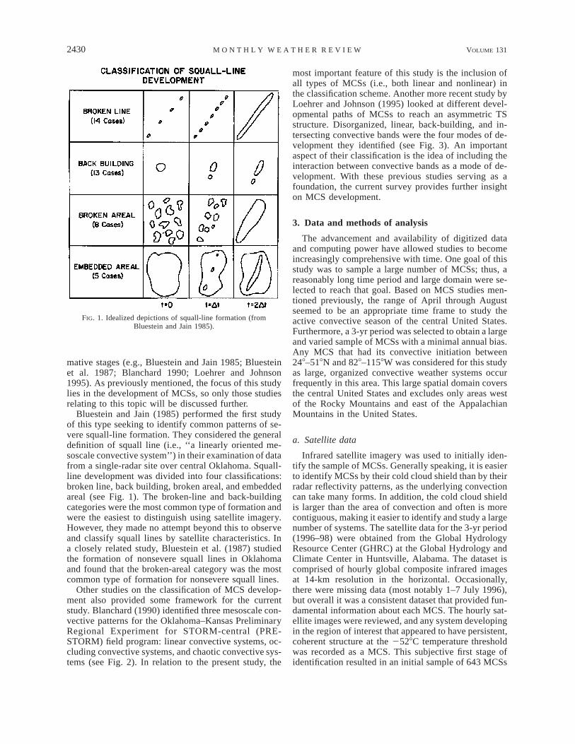
FIG. 4. Distribution of all MCSs by month.

considering the scale of convective radar echoes, andcloud shields grow much larger than the area of theunderlying convection. Systems with radar echoes of100 km or more in length seemed to generally havecloud shields of at least 30 000 km2 in area (approxi-mately the area of a circle with a radius of 100 km).The reexamination of the small systems also led to theconclusion that the most coherent systems maintainedan area of at least 30 000 km2. Thus, the size criterionfor the smaller systems was set at $30 000 km2 withthe caveat that their maximum size must be at least 50000 km2 as a way of connecting the definition of thesmaller systems to the larger systems. To keep the nam-ing convention as simple as possible, the smaller circularsystems are referred to as meso-b circular convectivesystems (MbCCSs) and the smaller linear systems arecalled meso-b elongated convective systems (MbECSs).From Orlanski’s (1975) definitions of meteorologicalscales, the larger and longer-lasting MCSs fit more ap-propriately into the meso-a scale while the smaller andshorter-lived MCSs fit more appropriately into the meso-b scale; hence, the reasoning for the nomenclature. Ta-ble 2 shows the definitions of the four classes of MCSsaccording to infrared satellite characteristics: MCC,PECS, MbCCS, and MbECS. The terminology used todenote different MCS life cycle stages is the same asdefined by Maddox (1980): initiation is the time whenthe MCS size definition is first met, maximum extent isthe time when the cold cloud shield reaches a maximumsize, and termination occurs when the MCS no longersatisfies its size definition.

b. Basic characteristics

As discussed in section 3, 514 systems were identifiedand subjected to the satellite classification scheme. Dur-ing the classification process, 49 systems were removedfrom consideration for not meeting the definition of oneof the satellite categories, which left 465 classifiableMCSs.

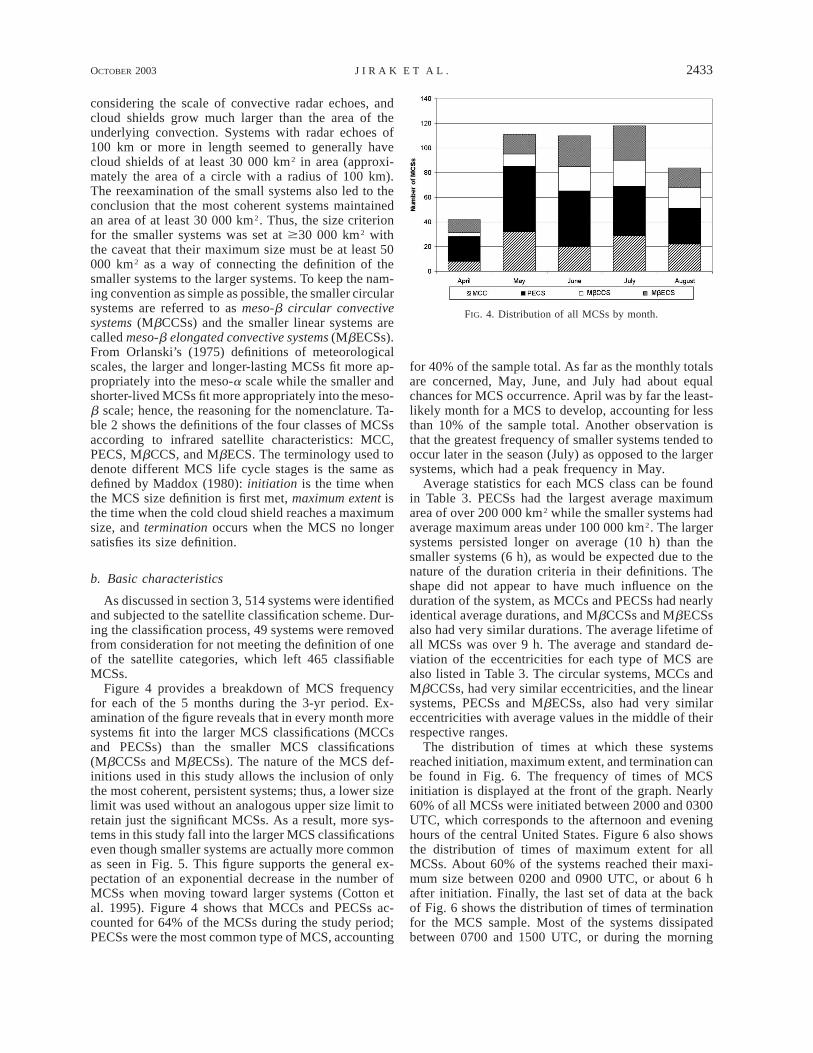
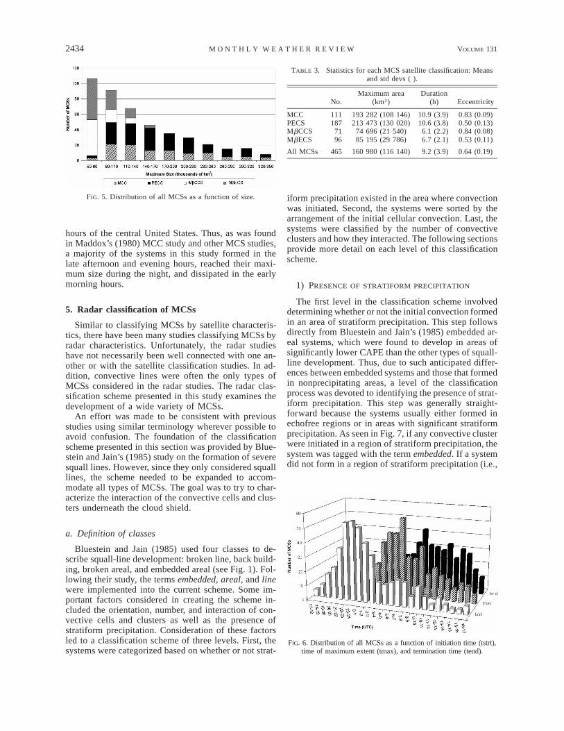
Figure 4 provides a breakdown of MCS frequencyfor each of the 5 months during the 3-yr period. Ex-amination of the figure reveals that in every month moresystems fit into the larger MCS classifications (MCCsand PECSs) than the smaller MCS classifications(MbCCSs and MbECSs). The nature of the MCS def-initions used in this study allows the inclusion of onlythe most coherent, persistent systems; thus, a lower sizelimit was used without an analogous upper size limit toretain just the significant MCSs. As a result, more sys-tems in this study fall into the larger MCS classificationseven though smaller systems are actually more commonas seen in Fig. 5. This figure supports the general ex-pectation of an exponential decrease in the number ofMCSs when moving toward larger systems (Cotton etal. 1995). Figure 4 shows that MCCs and PECSs ac-counted for 64% of the MCSs during the study period;PECSs were the most common type of MCS, accounting

for 40% of the sample total. As far as the monthly totalsare concerned, May, June, and July had about equalchances for MCS occurrence. April was by far the least-likely month for a MCS to develop, accounting for lessthan 10% of the sample total. Another observation isthat the greatest frequency of smaller systems tended tooccur later in the season (July) as opposed to the largersystems, which had a peak frequency in May.

Average statistics for each MCS class can be foundin Table 3. PECSs had the largest average maximumarea of over 200 000 km2 while the smaller systems hadaverage maximum areas under 100 000 km2. The largersystems persisted longer on average (10 h) than thesmaller systems (6 h), as would be expected due to thenature of the duration criteria in their definitions. Theshape did not appear to have much influence on theduration of the system, as MCCs and PECSs had nearlyidentical average durations, and MbCCSs and MbECSsalso had very similar durations. The average lifetime ofall MCSs was over 9 h. The average and standard de-viation of the eccentricities for each type of MCS arealso listed in Table 3. The circular systems, MCCs andMbCCSs, had very similar eccentricities, and the linearsystems, PECSs and MbECSs, also had very similareccentricities with average values in the middle of theirrespective ranges.

The distribution of times at which these systemsreached initiation, maximum extent, and termination canbe found in Fig. 6. The frequency of times of MCSinitiation is displayed at the front of the graph. Nearly60% of all MCSs were initiated between 2000 and 0300UTC, which corresponds to the afternoon and eveninghours of the central United States. Figure 6 also showsthe distribution of times of maximum extent for allMCSs. About 60% of the systems reached their maxi-mum size between 0200 and 0900 UTC, or about 6 hafter initiation. Finally, the last set of data at the backof Fig. 6 shows the distribution of times of terminationfor the MCS sample. Most of the systems dissipatedbetween 0700 and 1500 UTC, or during the morning


FIG. 5. Distribution of all MCSs as a function of size.

TABLE 3. Statistics for each MCS satellite classification: Meansand std devs ( ).

No.Maximum area

(km2)Duration

(h) Eccentricity

MCCPECSMbCCSMbECS

111187

7196

193 282 (108 146)213 473 (130 020)

74 696 (21 540)85 195 (29 786)

10.9 (3.9)10.6 (3.8)

6.1 (2.2)6.7 (2.1)

0.83 (0.09)0.50 (0.13)0.84 (0.08)0.53 (0.11)

All MCSs 465 160 980 (116 140) 9.2 (3.9) 0.64 (0.19)

FIG. 6. Distribution of all MCSs as a function of initiation time (tstrt),time of maximum extent (tmax), and termination time (tend).

hours of the central United States. Thus, as was foundin Maddox’s (1980) MCC study and other MCS studies,a majority of the systems in this study formed in thelate afternoon and evening hours, reached their maxi-mum size during the night, and dissipated in the earlymorning hours.

5. Radar classification of MCSs

Similar to classifying MCSs by satellite characteris-tics, there have been many studies classifying MCSs byradar characteristics. Unfortunately, the radar studieshave not necessarily been well connected with one an-other or with the satellite classification studies. In ad-dition, convective lines were often the only types ofMCSs considered in the radar studies. The radar clas-sification scheme presented in this study examines thedevelopment of a wide variety of MCSs.

An effort was made to be consistent with previousstudies using similar terminology wherever possible toavoid confusion. The foundation of the classificationscheme presented in this section was provided by Blue-stein and Jain’s (1985) study on the formation of severesquall lines. However, since they only considered squalllines, the scheme needed to be expanded to accom-modate all types of MCSs. The goal was to try to char-acterize the interaction of the convective cells and clus-ters underneath the cloud shield.

a. Definition of classes

Bluestein and Jain (1985) used four classes to de-scribe squall-line development: broken line, back build-ing, broken areal, and embedded areal (see Fig. 1). Fol-lowing their study, the terms embedded, areal, and linewere implemented into the current scheme. Some im-portant factors considered in creating the scheme in-cluded the orientation, number, and interaction of con-vective cells and clusters as well as the presence ofstratiform precipitation. Consideration of these factorsled to a classification scheme of three levels. First, thesystems were categorized based on whether or not strat-

iform precipitation existed in the area where convectionwas initiated. Second, the systems were sorted by thearrangement of the initial cellular convection. Last, thesystems were classified by the number of convectiveclusters and how they interacted. The following sectionsprovide more detail on each level of this classificationscheme.

1) PRESENCE OF STRATIFORM PRECIPITATION

The first level in the classification scheme involveddetermining whether or not the initial convection formedin an area of stratiform precipitation. This step followsdirectly from Bluestein and Jain’s (1985) embedded ar-eal systems, which were found to develop in areas ofsignificantly lower CAPE than the other types of squall-line development. Thus, due to such anticipated differ-ences between embedded systems and those that formedin nonprecipitating areas, a level of the classificationprocess was devoted to identifying the presence of strat-iform precipitation. This step was generally straight-forward because the systems usually either formed inechofree regions or in areas with significant stratiformprecipitation. As seen in Fig. 7, if any convective clusterwere initiated in a region of stratiform precipitation, thesystem was tagged with the term embedded. If a systemdid not form in a region of stratiform precipitation (i.e.,


FIG. 7. Idealized depiction of the three-level classification schemeused to categorize MCS development as seen by radar. The solid linesand contours represent relative reflectivity levels while the dashedlines represent the outline of the cold cloud shield.

not embedded), it was not given a label for this levelof the classification scheme.

2) ARRANGEMENT OF CONVECTIVE CELLS

The next level in the classification scheme describedthe arrangement of convective cells at initiation. Onceagain, this follows closely from Bluestein and Jain(1985) who categorized cellular arrangement into lineand areal categories. Thus, this step involved analyzingthe early stages of convection to determine whether ornot the cells were arranged in a line. Figure 7 showsthat systems with convection organized in a linear fash-ion received the term line while systems with scatteredconvection (i.e., not arranged linearly) received the termareal. If a system were comprised of convective clusterswith both types of cellular arrangement, it was giventhe term combination. Keep in mind that this step doesnot necessarily provide information on the shape of theMCS at its maturity. As Bluestein and Jain (1985)showed, areal systems can develop into squall lines.

3) INTERACTION OF CONVECTIVE CLUSTERS

The final level in the classification scheme involvedobserving how the convective cells grew into clustersand interacted with other convective clusters. This nec-essarily involved stages later into the life cycle of theMCSs (generally to about the time of maximum extent)and was the most subjective step in the classificationscheme. The term cluster referred to a meso-b groupingof convective cells that were contiguous or nearly con-tiguous. Independent convective clusters were distin-guished from one another by physical separation be-tween convection, difference in orientation from sur-rounding convection, and initiation of convection at dif-ferent times. Three major features of cluster interactionemerged, and the systems were categorized accordingly.One type of interaction involved the growth of convec-tive cells into a single convective cluster. These systemswere termed isolated systems (see Fig. 7). Another typeof interaction involved the development of multiple in-dependent convective clusters that merged into a singleentity. These systems were given the name merger sys-tems. Finally, if individual convective clusters devel-oped close enough to one another to share a commoncloud shield, but did not physically merge as seen byradar, then they were termed nonmerger systems. Thenonmerger systems appear the same as merger systemswhen viewed by satellite imagery; however, examina-tion of radar imagery reveals that they are very differentin the fact that the underlying convective clusters donot merge together. Consequently, both satellite and ra-dar data must be examined to classify these systems,which is a feature unique to this study that was not apart of previous MCS studies.

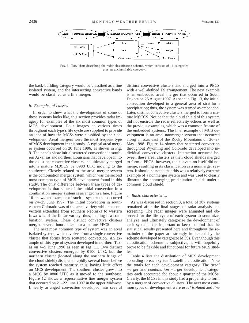
The nature of the classification scheme as seen in Fig.8 leads to 17 categories, including an unclassifiable cat-

egory and four combination categories. The unclassi-fiable category contains systems that could not be clas-sified in one or more of the levels of classificationscheme. The combination categories arise from systemswith clusters that develop from a mixture of line andareal arrangements. Also, note that isolated systems can-not have a combination category since they developfrom a single convective cluster. Of course, not all cat-egories are guaranteed to include many systems sincethis was a classification process, rather than just a listof the most important categories.

To illustrate the flexibility and usefulness of this newscheme, it will be used to classify the various categoriesfrom previous MCS development studies. From Blue-stein and Jain’s (1985) study (Fig. 1): the broken-linecategory would be classified as a line isolated system,the back-building category would also be classified asa line isolated system, the broken areal category wouldbe classified as an areal isolated system, and the em-bedded areal category would be classified as an em-bedded areal isolated system. From Blanchard’s (1990)study (Fig. 2): the linear convective system would beclassified as a line isolated system, the occluding con-vective system would be classified as a line merger, andthe chaotic convective system (as represented in thefigure without widespread stratiform precipitation)would be classified as an areal nonmerger. From Loehrerand Johnson (1995) (Fig. 3): the linear system wouldbe classified as a line isolated system, the disorganizedsystem would be classified as an areal isolated system,


FIG. 8. Flow chart describing the radar classification scheme, which consists of 16 categoriesplus an unclassifiable category.

the back-building category would be classified as a lineisolated system, and the intersecting convective bandswould be classified as a line merger.

b. Examples of classes

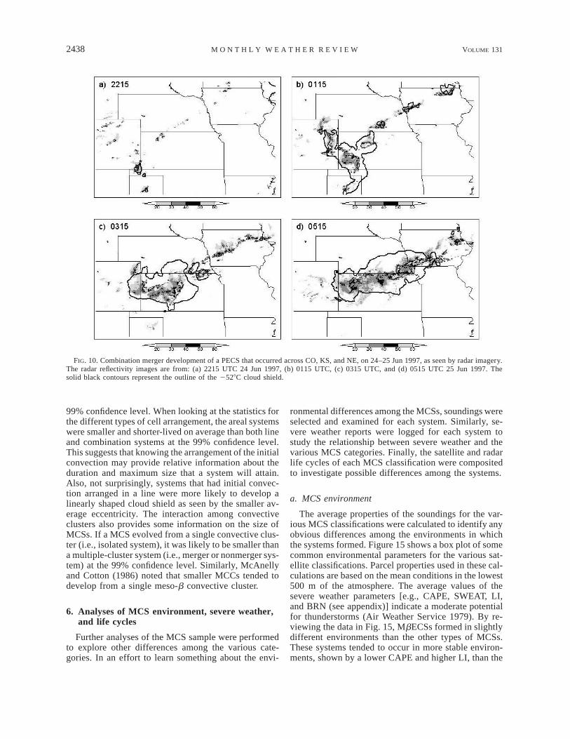
In order to show what the development of some ofthese systems looks like, this section provides radar im-agery for examples of the six most common types ofMCS development. Four images at various timesthroughout each type’s life cycle are supplied to providean idea of how the MCSs were classified by their de-velopment. Areal mergers were the most frequent typeof MCS development in this study. A typical areal merg-er system occurred on 20 June 1996, as shown in Fig.9. The panels show initial scattered convection in south-ern Arkansas and northern Louisiana that developed intothree distinct convective clusters and ultimately mergedinto a mature MbCCS by 0900 UTC moving to thesouthwest. Closely related to the areal merger systemis the combination merger system, which was the secondmost common type of MCS development found in thisstudy. The only difference between these types of de-velopment is that some of the initial convection in acombination merger system is arranged in a line. Figure10 shows an example of such a system that occurredon 24–25 June 1997. The initial convection in south-eastern Colorado was of the areal variety while the con-vection extending from southern Nebraska to westernIowa was of the linear variety, thus, making it a com-bination system. These distinct convective clustersmerged several hours later into a mature PECS.

The next most common type of system was an arealisolated system, which evolves from a single convectivecluster that forms from scattered convection. An ex-ample of this type of system developed in northern Tex-as on 4–5 June 1996 as seen in Fig. 11. Two distinctconvective clusters emerged by 0100 UTC, but thenorthern cluster (located along the northern fringe ofthe cloud shield) dissipated rapidly several hours beforethe system reached maturity, thus, having little effecton MCS development. The southern cluster grew intoa MCC by 0800 UTC as it moved to the southeast.Figure 12 shows a representative line merger systemthat occurred on 21–22 June 1997 in the upper Midwest.Linearly arranged convection developed into several

distinct convective clusters and merged into a PECSwith a well-defined TS arrangement. The next exampleis an embedded areal merger that occurred in SouthDakota on 25 August 1997. As seen in Fig. 13, the initialconvection developed in a general area of stratiformprecipitation; thus, the system was termed as embedded.Later, distinct convective clusters merged to form a ma-ture MbCCS. Notice that the cloud shield of this systemdid not encircle the radar reflectivity echoes as well asthe previous examples, which was a common feature ofthe embedded systems. The final example of MCS de-velopment is an areal nonmerger system that occurredalong an axis east of the Rocky Mountains on 26–27May 1998. Figure 14 shows that scattered convectionthroughout Wyoming and Colorado developed into in-dividual convective clusters. Interaction occurred be-tween these areal clusters as their cloud shields mergedto form a PECS; however, the convection itself did notmerge, resulting in its classification as a nonmerger sys-tem. It should be noted that this was a relatively extremeexample of a nonmerger system and was used to clearlyillustrate the nonmerging precipitation shields under acommon cloud shield.

c. Basic characteristics

As was discussed in section 3, a total of 387 systemsremained after the final stages of radar analysis andscreening. The radar images were animated and ob-served for the life cycle of each system to scrutinize,analyze, and ultimately categorize the development ofeach system. It is important to keep in mind that thestatistical results presented here and throughout the re-mainder of the paper are strongly influenced by thescheme developed to categorize MCSs. Even though thisclassification scheme is subjective, it will hopefullyprove to be flexible and functional for future MCS stud-ies.

Table 4 lists the distribution of MCS developmentaccording to each system’s satellite classification. Notethe totals for each development category. The arealmerger and combination merger development catego-ries each accounted for about a quarter of the MCSs.Clearly, the MCSs in this study had a propensity to formby a merger of convective clusters. The next most com-mon types of development were areal isolated and line


FIG. 9. Areal merger development of a MbCCS that occurred in southern Arkansas and northern Louisiana on 20 Jun 1996, as seen byradar imagery. The radar reflectivity images are from: (a) 0000, (b) 0200, (c) 0400, and (d) 0900 UTC. The solid black contours representthe outline of the 2528C cloud shield.

merger categories. However, each of these categoriesonly accounted for less than 10% of the total MCSsample. Also, it is obvious that the embedded nonmergersystems were not significant types of development inthis sample.

Another method that makes it easier to view the re-sults is to break the data into the three levels of theclassification scheme. Table 5 presents the data in thisfashion. First, note that embedded systems accountedfor only 17% of the total MCS sample. A higher per-centage (21%) of the smaller satellite-defined systems(MbCCSs and MbECSs) were embedded, compared tothe larger systems (14% of MCCs and PECSs). Themiddle section of Table 5 shows that more than half ofthe systems had initial convection arranged in an arealfashion. Not too surprisingly, the systems with elon-gated cloud shields at their maximum extent (PECS andMbECSs) were more likely to have linearly arrangedconvection at initiation than the circular systems (MCCsand MbCCSs). Finally, merger systems were by far themost common type of cluster interaction accounting forthe development of over 70% of the MCSs. Althoughthe nonmerger systems are a distinct class of MCS de-velopment, they only occurred about 8% of the time.The data also show that single-cluster, or isolated, sys-

tems accounted for a higher frequency of developmentinto smaller systems (MbCCSs and MbECSs). Aboutone-fourth of the meso-b systems were isolated systemswhile only 15% of the larger systems consisted of asingle convective cluster.

A couple of features appear when examining the dis-tribution of MCS development by month. Inspection ofthe presence of stratiform precipitation reveals that 13of the 36 MCSs in April, or 36%, were embedded, ascompared to only 15% of the total number of systemsthroughout the remainder of the convective season (i.e.,52 out of 351). The month of April also stands out whenconsidering the arrangement of convective cells. Due tothe strong baroclinic forcing early in the season, one-third of all April MCSs (12 out of 36) developed in alinear fashion while only 15% of the systems fell intothe line category throughout the rest of the convectiveseason.

The satellite life cycle statistics for each level of radardevelopment are provided in Table 6. Confidence levelswere calculated using the Student’s t test to show sta-tistically significant differences among the properties ofvarious MCS categories. MCSs that were initiated instratiform precipitation developed into smaller systemsat maturity than MCSs that developed in clear air at the


FIG. 10. Combination merger development of a PECS that occurred across CO, KS, and NE, on 24–25 Jun 1997, as seen by radar imagery.The radar reflectivity images are from: (a) 2215 UTC 24 Jun 1997, (b) 0115 UTC, (c) 0315 UTC, and (d) 0515 UTC 25 Jun 1997. Thesolid black contours represent the outline of the 2528C cloud shield.

99% confidence level. When looking at the statistics forthe different types of cell arrangement, the areal systemswere smaller and shorter-lived on average than both lineand combination systems at the 99% confidence level.This suggests that knowing the arrangement of the initialconvection may provide relative information about theduration and maximum size that a system will attain.Also, not surprisingly, systems that had initial convec-tion arranged in a line were more likely to develop alinearly shaped cloud shield as seen by the smaller av-erage eccentricity. The interaction among convectiveclusters also provides some information on the size ofMCSs. If a MCS evolved from a single convective clus-ter (i.e., isolated system), it was likely to be smaller thana multiple-cluster system (i.e., merger or nonmerger sys-tem) at the 99% confidence level. Similarly, McAnellyand Cotton (1986) noted that smaller MCCs tended todevelop from a single meso-b convective cluster.

6. Analyses of MCS environment, severe weather,and life cycles

Further analyses of the MCS sample were performedto explore other differences among the various cate-gories. In an effort to learn something about the envi-

ronmental differences among the MCSs, soundings wereselected and examined for each system. Similarly, se-vere weather reports were logged for each system tostudy the relationship between severe weather and thevarious MCS categories. Finally, the satellite and radarlife cycles of each MCS classification were compositedto investigate possible differences among the systems.

a. MCS environment

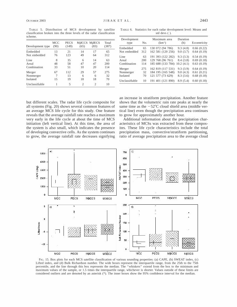
The average properties of the soundings for the var-ious MCS classifications were calculated to identify anyobvious differences among the environments in whichthe systems formed. Figure 15 shows a box plot of somecommon environmental parameters for the various sat-ellite classifications. Parcel properties used in these cal-culations are based on the mean conditions in the lowest500 m of the atmosphere. The average values of thesevere weather parameters [e.g., CAPE, SWEAT, LI,and BRN (see appendix)] indicate a moderate potentialfor thunderstorms (Air Weather Service 1979). By re-viewing the data in Fig. 15, MbECSs formed in slightlydifferent environments than the other types of MCSs.These systems tended to occur in more stable environ-ments, shown by a lower CAPE and higher LI, than the


FIG. 11. Areal isolated development of a MCC that occurred in northern TX on 4–5 Jun 1996, as seen by radar imagery. The radarreflectivity images are from: (a) 2130 UTC 4 Jun 1996, (b) 0100 UTC, (c) 0315 UTC, and (d) 0800 UTC 5 Jun 1996. The solid blackcontours represent the outline of the 2528C cloud shield.

other satellite categories. The SWEAT index shows astatistical difference between the larger MCSs (MCCsand PECSs) and the smaller systems (MbCCS andMbECS). At the 95% confidence level, the smallerMCSs had a lower average SWEAT index than the largersystems. This indicates that the SWEAT index, whichwas created to help forecast tornadic thunderstorms byincluding wind shear in its formulation (see appendix),may provide some information about the maximum sizeof a MCS. Forty-three percent of the larger systems hada SWEAT index greater than 350 while only one-fourthof the smaller systems had a SWEAT index of 350 orgreater. A more in-depth analysis of the individual termsof the SWEAT index revealed that MbCCSs andMbECSs had lower SWEAT indices than the larger sys-tems for different reasons. MbCCSs had a lower averageSWEAT index because each of the five terms wereslightly lower while the MbECSs had a lower averageSWEAT index because the Total Totals and 850-mbdewpoint terms were much lower than those of the largersystems.

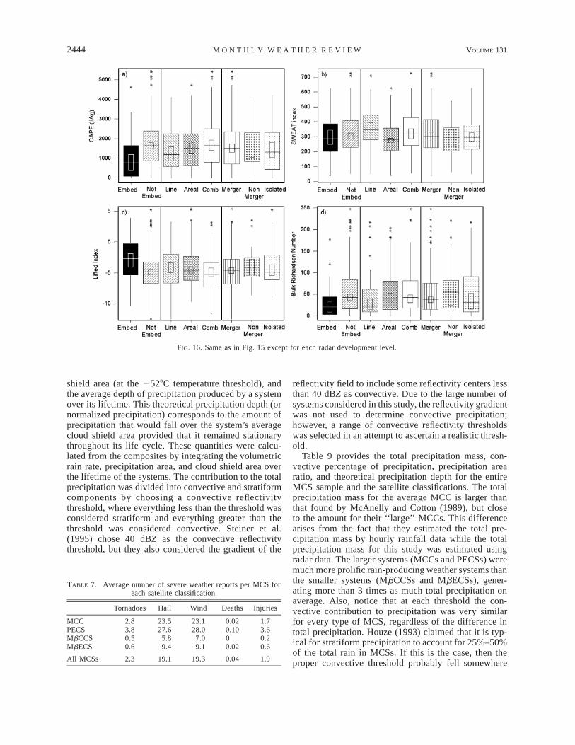
In a similar manner, Fig. 16 contains average sound-ing properties for each radar classification of MCS de-velopment. This figure reveals a significant differencebetween the environments of embedded systems andthose that do not form in areas of stratiform precipita-tion. As expected, the environments of embedded sys-

tems were much more stable as shown by a lower CAPEand higher LI at greater than the 99% confidence level.The sounding average differences, however, were muchless pronounced when dividing the systems accordingto their cell arrangement and cluster interaction. Arealsystems did have a statistically lower average SWEATindex than line and combination systems at the 95%confidence level. An examination of the individualterms of the SWEAT index indicates that the areal sys-tems had a much lower directional shear term than sys-tems with linearly arranged convection, which indicatesthe dynamically different environments that producedthese systems.

b. Severe weather reports

The inspection of the stability parameters for thesesystems leads directly into the discussion of severeweather. MCSs are convective, of course, by definition,so one might expect severe weather from these systems,but do certain types of systems have a propensity toproduce severe weather? Table 7 provides the averagenumber of severe weather reports for each satellite clas-sification per MCS for tornadoes, hail, and wind as wellas deaths and injuries. To be reported as severe weather,a tornado must merely be present, hail must be ¾ in.in diameter or larger, and winds must be measured at


FIG. 12. Line merger development of a PECS that occurred in the upper Midwest on 21–22 Jun 1997, as seen by radar imagery. The radarreflectivity images are from: (a) 2000 UTC, (b) 2200 UTC, (c) 2315 UTC 21 Jun 1997, and (d) 0100 UTC 22 Jun 1997. The solid blackcontours represent the outline of the 2528C cloud shield.

greater than 50 kt at the surface. Certainly, it is impor-tant to keep in mind that population density and thenumber of objects that can be damaged (e.g., trees andbuildings) may have an effect on the number of severeweather incidents that are reported. MCCs and PECSsaccounted for most of the severe weather reports duringthe study period including about three tornadoes and 25wind and hail reports per system. The smaller systems(MbCCSs and MbECSs) had many fewer severe weath-er reports per system with less than one tornado andabout eight wind and hail reports. More than half of allsevere weather reports and almost three-quarters of thereported deaths and injuries were due to PECSs eventhough the average severe weather indices did not showthem to develop in significantly different environmentsfrom the other types of MCSs. This information rein-forces the importance of PECSs as a common and vi-olent weather system. These systems are the most severeMCS overall; however, they are not necessarily moresevere per unit area than the other MCSs. When thenumber of severe weather reports for each system isnormalized by its integrated cloud shield area through-out its life cycle, the different systems generated a sim-ilar number of severe weather reports per unit area perunit time (Fig. 17). The larger systems, though, werestill more likely to produce tornadoes, as they had a

nonzero median value of normalized tornado reports.Thus, the larger systems produced more severe weatherreports per system primarily due to their larger size andlonger duration.

In a similar fashion, the severe weather reports canbe classified according to the radar developmental char-acteristics of each system to investigate the relationshipbetween development and the occurrence of severeweather. Table 8 lists the average number of severeweather reports for each level of development and Fig.18 shows the normalized severe weather reports for eachcategory. As expected due to the environmental differ-ences between embedded and nonembedded systems,severe weather was much more frequent with systemsthat were not embedded from an overall and normalizedviewpoint. The areal systems also stand out as they gen-erated significantly less severe weather than line andcombination systems, which is shown by the fewer num-ber of average and normalized severe weather reportsper MCS. This agrees with the findings of Bluestein etal. (1987) that broken areal squall lines are the leastlikely development category to be associated with se-vere weather. Therefore, the arrangement of the initialconvection may provide some information on the abilityof the system to produce severe weather. Note that sys-tems with linearly arranged convection (i.e., line and


FIG. 13. Embedded areal merger development of a MbCCS that occurred in South Dakota on 25 Aug 1997, as seen by radar imagery.The radar reflectivity images are from: (a) 0100, (b) 0345, (c) 0645, and (d) 1045 UTC. The solid black contours represent the outline ofthe 2528C cloud shield.

combination systems) produced a high frequency ofwind reports, which is consistent with the bow echorelationship to derechos (Johns and Hirt 1987). Lookingat the cluster interaction categories, the merger systemstended to have more severe weather reports than non-merger and isolated systems per system, but Fig. 18shows that all of the cluster interaction categories pro-duced a similar number of severe weather reports perunit area per unit time.

c. MCS satellite life cycle

The life cycles of the various MCS classificationswere combined, or composited, to allow for a generaloverview of each category’s life cycle. The systemswere composited by normalizing the life cycle of eachsystem according to the average growth stage (initiationto maximum extent) and the average dissipation stage(maximum extent to termination) for each MCS cate-gory. This normalization allows systems of all dura-tions, growth rates, and decay rates to be composited.The areas of the 2528, 2588, 2648, and 2708C black-body temperature thresholds were averaged at each nor-malized MCS time in order to create a composite life-cycle. Figure 19 shows the composite for the entire MCS

sample. In this figure, the areas of the aforementionedIR temperature thresholds are plotted against the MCStimescale with ‘‘00’’ representing the initiation of thesystems, as demarcated by a vertical line. The middlevertical line indicates the time of maximum extent ofthe composite; thus, the period between these first twolines represents the growth stage of the systems. Thevertical line on the right signifies the termination of thesystems, so the period between the second two linesrepresents the decay stage of the systems.

The satellite life cycles of each MCS category hadvery similar features with the scale being the primarydifference among the life cycles. One common featuredisplayed in Fig. 19 and found in all of the satellitecomposites is that the areas of colder temperature thresh-olds reach a maximum before the warmer thresholds.For example, Fig. 19 shows that the area of the 2588Ccloud shield peaks before the 2528C area reaches amaximum. In addition, the growth stage of MCSs gen-erally lasts an hour longer than the decay stage.

d. MCS radar life cycle

The normalized MCS timescale developed to producecomposite satellite life cycles was also used to create


FIG. 14. Areal nonmerger development of a PECS that occurred east of the Rocky Mountains on 26–27 May 1998, as seen by radarimagery. The radar reflectivity images are from: (a) 2045 UTC, and (b) 2245 UTC 26 May 1998, (c) 0045 UTC, and (d) 0245 UTC 27 May1998. The solid black contours represent the outline of the 2528C cloud shield.

TABLE 4. Distribution of MCS radar development by satellite classification.

Development type MCC PECS MbCCS MbECS Total

Embedded line mergerEmbedded areal mergerEmbedded combination mergerEmbedded line nonmergerEmbedded areal nonmerger

16300

46700

07100

16401

62515

01

Embedded combination nonmergerEmbedded line isolatedEmbedded areal isolatedLine mergerAreal merger

0034

26

013

2034

0242

20

0145

25

04

1431

105Combination mergerLine nonmergerAreal nonmergerCombination nonmerger

27043

41373

9060

16140

934

216

Line isolatedAreal isolatedUnclassifiable

391

785

210

2

672

183410

Total 90 149 65 83 387

composite radar life cycle plots. Thus, the vertical linesin Fig. 20 still represent the start, maximum, and endtimes of the satellite life cycle. There are three curvesplotted in these figures: the solid curve represents sys-tem-total volumetric rain rate, V, calculated using theWSR-080 default Z–R relationship as described in sec-

tion 3; the thick, dashed curve represents the precipi-tation area, A (defined as the reflectivity area $ 20 dBZ);and the thin, dashed curve represents the average rainrate, , which is calculated as 5 V/A.R R

The radar life cycle plots for each MCS category werealso very much alike with similar trends and properties,


TABLE 5. Distribution of MCS development by satelliteclassification broken into the three levels of the radar classificationscheme.

Development typeMCC(90)

PECS(149)

MbCCS(65)

MbECS(83)

Total(387)

EmbeddedNot embedded

1376

21123

1449

1764

65312

LineArealCombination

84833

355851

64710

144720

63200114

MergerNonmergerIsolated

677

15

1121319

296

18

576

18

2753270

Unclassifiable 1 5 2 2 10

TABLE 6. Statistics for each radar development level: Means andstd devs ( ).

Developmenttype No.

Maximum area(km2)

Duration(h) Eccentricity


65312

130 072 (94 786)162 581 (120 256)

9.3 (4.8)9.0 (3.7)

0.66 (0.22)0.64 (0.19)


63200114

191 393 (122 282)129 768 (96 761)185 688 (133 784)

9.3 (3.3)8.4 (3.8)

10.2 (4.1)

0.54 (0.19)0.69 (0.18)0.63 (0.19)


2753270

162 819 (117 531)184 195 (165 548)121 577 (73 629)

9.3 (3.9)9.0 (4.3)8.3 (3.6)

0.64 (0.19)0.61 (0.21)0.68 (0.18)

Unclassifiable 10 191 401 (121 890) 8.9 (5.4) 0.60 (0.18)

FIG. 15. Box plots for each MCS satellite classification of various sounding properties: (a) CAPE, (b) SWEAT index, (c)Lifted index, and (d) Bulk Richardson number. The wide boxes represent the interquartile range, from the 25th to the 75thpercentile, and the line through this box represents the median. The ‘‘whiskers’’ extend from the box to the minimum andmaximum values of the sample, or 1.5 times the interquartile range, whichever is shorter. Values outside of these limits areconsidered outliers and are denoted by an asterisk (*). The inner boxes show the 95% confidence interval for the median.

but different scales. The radar life cycle composite forall systems (Fig. 20) shows several common features ofan average MCS life cycle for this study. One featurereveals that the average rainfall rate reaches a maximumvery early in the life cycle at about the time of MCSinitiation (left vertical line). At this time, the area ofthe system is also small, which indicates the presenceof developing convective cells. As the system continuesto grow, the average rainfall rate decreases signifying

an increase in stratiform precipitation. Another featureshows that the volumetric rain rate peaks at nearly thesame time as the 2528C cloud shield area (middle ver-tical line) even though the precipitation area continuesto grow for approximately another hour.

Additional information about the precipitation char-acteristics of MCSs was extracted from these compos-ites. These life cycle characteristics include the totalprecipitation mass, convective/stratiform partitioning,ratio of average precipitation area to the average cloud


FIG. 16. Same as in Fig. 15 except for each radar development level.

TABLE 7. Average number of severe weather reports per MCS foreach satellite classification.

Tornadoes Hail Wind Deaths Injuries

MCCPECSMbCCSMbECS

2.83.80.50.6

23.527.6

5.89.4

23.128.0

7.09.1

0.020.1000.02

1.73.60.20.6

All MCSs 2.3 19.1 19.3 0.04 1.9

shield area (at the 2528C temperature threshold), andthe average depth of precipitation produced by a systemover its lifetime. This theoretical precipitation depth (ornormalized precipitation) corresponds to the amount ofprecipitation that would fall over the system’s averagecloud shield area provided that it remained stationarythroughout its life cycle. These quantities were calcu-lated from the composites by integrating the volumetricrain rate, precipitation area, and cloud shield area overthe lifetime of the systems. The contribution to the totalprecipitation was divided into convective and stratiformcomponents by choosing a convective reflectivitythreshold, where everything less than the threshold wasconsidered stratiform and everything greater than thethreshold was considered convective. Steiner et al.(1995) chose 40 dBZ as the convective reflectivitythreshold, but they also considered the gradient of the

reflectivity field to include some reflectivity centers lessthan 40 dBZ as convective. Due to the large number ofsystems considered in this study, the reflectivity gradientwas not used to determine convective precipitation;however, a range of convective reflectivity thresholdswas selected in an attempt to ascertain a realistic thresh-old.

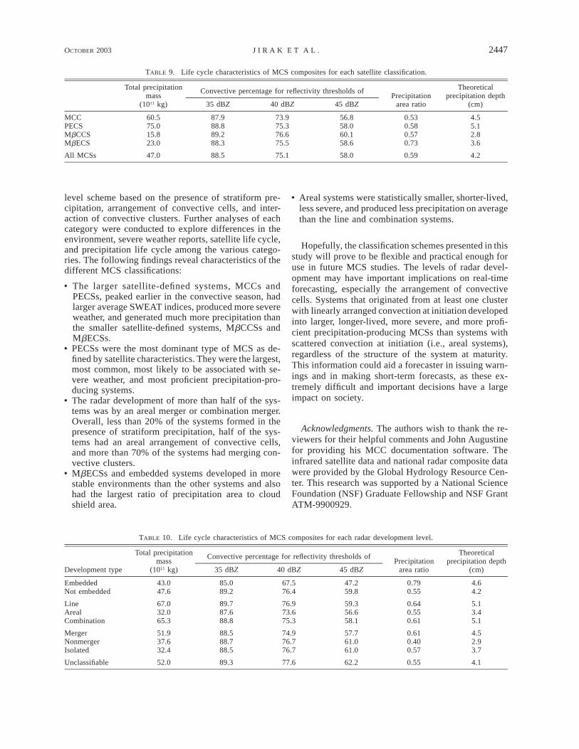
Table 9 provides the total precipitation mass, con-vective percentage of precipitation, precipitation arearatio, and theoretical precipitation depth for the entireMCS sample and the satellite classifications. The totalprecipitation mass for the average MCC is larger thanthat found by McAnelly and Cotton (1989), but closeto the amount for their ‘‘large’’ MCCs. This differencearises from the fact that they estimated the total pre-cipitation mass by hourly rainfall data while the totalprecipitation mass for this study was estimated usingradar data. The larger systems (MCCs and PECSs) weremuch more prolific rain-producing weather systems thanthe smaller systems (MbCCSs and MbECSs), gener-ating more than 3 times as much total precipitation onaverage. Also, notice that at each threshold the con-vective contribution to precipitation was very similarfor every type of MCS, regardless of the difference intotal precipitation. Houze (1993) claimed that it is typ-ical for stratiform precipitation to account for 25%–50%of the total rain in MCSs. If this is the case, then theproper convective threshold probably fell somewhere


FIG. 17. Same as in Fig. 15 except for the normalized severe weather reports: (a) hail, (b) wind, and (c) tornado. The normalized valuesare the number of reports per 104 km2 of the cold cloud shield area per hour.

TABLE 8. Average number of severe weather reports per MCS foreach radar development level.

Developmenttype Tornadoes Hail Wind Deaths Injuries


1.02.6

11.320.7

12.220.5

00.05

0.63.4


3.11.43.6

24.014.025.3

33.69.6

27.5

0.050.010.10

0.52.23.6


2.51.81.7

20.416.614.9

20.812.914.8

0.0500.03

1.80.92.9

Unclassifiable 2.6 20.4 27.6 0 2.5

between 40 and 45 dBZ for this MCS sample. The com-posite of all MCSs shows that on average almost 60%of the cold cloud shield area had underlying precipi-tation. MbECSs were the only type of MCS to varysignificantly from that percentage, as nearly ¾ of thecloud shield produced precipitation. However, these sys-tems still did not produce as much normalized precip-itation as MCCs and PECSs. PECSs were once againthe most impressive systems producing an average the-oretical precipitation depth of over 5 cm.

Similarly, Table 10 shows the total precipitation mass,convective percentage, precipitation area ratio, and the-

oretical precipitation depth for the levels of radar de-velopment. First of all, again notice that the convectivecontribution to precipitation was nearly identical for allcategories, except for the embedded systems. As ex-pected from their definition, these systems had a higherpercentage of stratiform precipitation as well as a highprecipitation area ratio. It is also noteworthy that em-bedded systems and MbECSs, which formed in the moststable environments, also had the highest ratio of pre-cipitation area to cloud shield area. Surprisingly, therewas not much difference in the total precipitation andnormalized precipitation between embedded systemsand those that did not develop in an area of stratiformprecipitation. This provides evidence that even thoughembedded systems may not generate a significantamount of severe weather, they are very important forthe production of precipitation over the agricultural re-gion of the central United States. Investigation of thecell arrangement categories shows that once again sys-tems with an areal arrangement of convective cells hadmuch different properties than systems with other typesof cellular arrangement. The areal systems producedmuch less total precipitation and also had much smallertheoretical precipitation depths than the line and com-bination categories. This indicates that areal systemswere relatively ineffective at producing precipitation.Finally, the interaction of convective clusters had a large


FIG. 18. Same as in Fig. 17 except for each radar development level.

FIG. 19. Infrared satellite life cycle composite for all systems.Curves (largest to smallest magnitudes) represent the areas of the2528, 2588, 2648, and 2708C blackbody temperature thresholds,respectively. Vertical lines represent the system initiation, maximumextent, and termination. Time is relative to system initiation.

FIG. 20. Radar life cycle composite for all systems. Solid curverepresents volumetric rain rate; thick, dashed curve represents pre-cipitation area; and thin, dashed curve represents average rain rate.Vertical lines represent initiation, maximum extent, and terminationof the satellite life cycle. Time is relative to system initiation.

influence on the ability of the MCSs to generate pre-cipitation. Systems with merging convective clustersproduced much more total and normalized precipitationthan isolated or nonmerger systems. As might be ex-pected from their definition as systems with nonmergingprecipitation shields under a common cloud shield, non-merger systems had a very low precipitation area ratioand produced less than 3 cm of rainfall on average.

7. Summary and conclusions

This study involved the identification and classifi-cation of several hundred MCSs by infrared satellitecharacteristics into four categories: MCCs, PECSs,MbCCSs, and MbECSs. In addition, the systems werereanalyzed with 2-km national composite radar reflec-tivity data to examine the developmental stages at ahigher spatial and temporal resolution. The radar de-velopment of each system was categorized by a three-


TABLE 9. Life cycle characteristics of MCS composites for each satellite classification.

Total precipitationmass

(1011 kg)

Convective percentage for reflectivity thresholds of

35 dBZ 40 dBZ 45 dBZPrecipitation

area ratio

Theoreticalprecipitation depth

(cm)

MCCPECSMbCCSMbECS

60.575.015.823.0

87.988.889.288.3

73.975.376.675.5

56.858.060.158.6

0.530.580.570.73

4.55.12.83.6

All MCSs 47.0 88.5 75.1 58.0 0.59 4.2

TABLE 10. Life cycle characteristics of MCS composites for each radar development level.

Development type

Total precipitationmass

(1011 kg)

Convective percentage for reflectivity thresholds of

35 dBZ 40 dBZ 45 dBZPrecipitation

area ratio

Theoreticalprecipitation depth

(cm)


43.047.6

85.089.2

67.576.4

47.259.8

0.790.55

4.64.2


67.032.065.3

89.787.688.8

76.973.675.3

59.356.658.1

0.640.550.61

5.13.45.1


51.937.632.4

88.588.788.5

74.976.776.7

57.761.061.0

0.610.400.57

4.52.93.7

Unclassifiable 52.0 89.3 77.6 62.2 0.55 4.1

level scheme based on the presence of stratiform pre-cipitation, arrangement of convective cells, and inter-action of convective clusters. Further analyses of eachcategory were conducted to explore differences in theenvironment, severe weather reports, satellite life cycle,and precipitation life cycle among the various catego-ries. The following findings reveal characteristics of thedifferent MCS classifications:

• The larger satellite-defined systems, MCCs andPECSs, peaked earlier in the convective season, hadlarger average SWEAT indices, produced more severeweather, and generated much more precipitation thanthe smaller satellite-defined systems, MbCCSs andMbECSs.

• PECSs were the most dominant type of MCS as de-fined by satellite characteristics. They were the largest,most common, most likely to be associated with se-vere weather, and most proficient precipitation-pro-ducing systems.

• The radar development of more than half of the sys-tems was by an areal merger or combination merger.Overall, less than 20% of the systems formed in thepresence of stratiform precipitation, half of the sys-tems had an areal arrangement of convective cells,and more than 70% of the systems had merging con-vective clusters.

• MbECSs and embedded systems developed in morestable environments than the other systems and alsohad the largest ratio of precipitation area to cloudshield area.

• Areal systems were statistically smaller, shorter-lived,less severe, and produced less precipitation on averagethan the line and combination systems.

Hopefully, the classification schemes presented in thisstudy will prove to be flexible and practical enough foruse in future MCS studies. The levels of radar devel-opment may have important implications on real-timeforecasting, especially the arrangement of convectivecells. Systems that originated from at least one clusterwith linearly arranged convection at initiation developedinto larger, longer-lived, more severe, and more profi-cient precipitation-producing MCSs than systems withscattered convection at initiation (i.e., areal systems),regardless of the structure of the system at maturity.This information could aid a forecaster in issuing warn-ings and in making short-term forecasts, as these ex-tremely difficult and important decisions have a largeimpact on society.

Acknowledgments. The authors wish to thank the re-viewers for their helpful comments and John Augustinefor providing his MCC documentation software. Theinfrared satellite data and national radar composite datawere provided by the Global Hydrology Resource Cen-ter. This research was supported by a National ScienceFoundation (NSF) Graduate Fellowship and NSF GrantATM-9900929.


APPENDIX

Sounding Indices

a. Bulk Richardson number (BRN)

2BRN 5 CAPE/(0.5U ),

where CAPE is the convective available potential en-ergy (m2 s22), U is the magnitude of the shear (u2 2u1, y 2 2 y1), u1, y1 is the average u, y in the lowest 500m, and u2, y 2 is the average u, y in the lowest 6000 m.

b. Lifted index (LI)

LI 5 T 2 T ,e500 p500

where Te500 is the environmental temperature in 8C at500 mb and Tp500 is the theoretical temperature in 8C aparcel of air would have at 500 mb if it were lifted dryadiabatically from the surface to its condensation level,thence moist adiabatically to 500 mb.

LI Thunderstorm potential

.2323 to 25

,25

WeakModerate

Strong

c. Total Totals (TT)

TT 5 T 2 T 2 2 3 T ,850 d850 500

where T850 is the temperature in 8C at 850 mb, Td850 isthe dewpoint temperature in 8C at 850 mb, and T500 isthe temperature in 8C at 500 mb.

TT Thunderstorm potential

,4545–55.55

WeakModerate

Strong

d. SWEAT index (SWEAT)

SWEAT 5 (12 3 T ) 1 [20 3 (TT 2 49)]d850

1 (2 3 W ) 1 W850 500

1 {125 3 [sin(D 2 D ) 1 0.2]},500 850

where Td850 is the dewpoint temperature in 8C at 850mb, TT is the Total Totals index and (TT 2 49) is setto zero if negative, W850 is the wind speed at 850 mbin knots, W500 is the wind speed at 500 mb in knots,D850 is the wind direction at 850 mb, and D500 is thewind direction at 500 mb.

SWEAT Thunderstorm potential

,300300–399400–599

.600

WeakModerate

StrongHigh

REFERENCES

Air Weather Service, 1979: The use of the skew T, log p diagram inanalysis and forecasting. Tech. Rep. AWS/TR-79/006, revised,157 pp. [Available from U.S. Air Force Air Weather Service,Scott Air Force Base, IL 62225-5008.]

Anderson, C. J., and R. W. Arritt, 1998: Mesoscale convective com-plexes and persistent elongated convective systems over theUnited States during 1992 and 1993. Mon. Wea. Rev., 126, 578–599.

Augustine, J. A., 1985: An automated method for the documentationof cloud-top characteristics of mesoscale convective systems.NOAA Tech. Memo. ERL ESG-10, Dept. of Commerce, Boulder,CO, 121 pp.

——, and K. W. Howard, 1988: Mesoscale convective complexesover the United States during 1985. Mon. Wea. Rev., 116, 685–701.

Blanchard, D. O., 1990: Mesoscale convective patterns of the south-ern High Plains. Bull. Amer. Meteor. Soc., 71, 994–1005.

Bluestein, H. B., and C. R. Parks, 1983: A synoptic and photographicclimatology of low-precipitation severe thunderstorms in thesouthern Plains. Mon. Wea. Rev., 111, 2034–2046.

——, and M. H. Jain, 1985: Formation of mesoscale lines of pre-cipitation: Severe squall lines in Oklahoma during the spring. J.Atmos. Sci., 42, 1711–1732.

——, G. T. Marx, and M. H. Jain, 1987: Formation of mesoscalelines of precipitation: Nonsevere squall lines in Oklahoma duringthe spring. Mon. Wea. Rev., 115, 2719–2727.

Brooks, R. H., C. A. Doswell, and J. Cooper, 1994: On the environ-ments of tornadic and nontornadic mesocyclones. Wea. Fore-casting, 9, 606–618.

Cotton, W. R., M. S. Lin, R. L. McAnelly, and C. J. Tremback, 1989:A composite model of mesoscale convective complexes. Mon.Wea. Rev., 117, 765–783.

——, G. D. Alexander, R. Hertenstein, R. L. Walko, R. L. McAnelly,and M. Nicholls, 1995: Cloud venting—A review and some newglobal annual estimates. Earth-Sci. Rev., 39, 169–206.

Fritsch, J. M., R. J. Kane, and C. R. Chelius, 1986: The contributionof mesoscale convective weather systems to the warm-seasonprecipitation in the United States. J. Climate Appl. Meteor., 25,1333–1345.

Fulton, R. A., J. P. Breidenbach, D.-J. Seo, D. A. Miller, and T.O’Bannon, 1998: The WSR-88D rainfall algorithm. Wea. Fore-casting, 13, 377–395.

Geerts, B., 1998: Mesoscale convective systems in the southeast Unit-ed States during 1994–95: A survey. Wea. Forecasting, 13, 860–869.

Hilgendorf, E. R., and R. H. Johnson, 1998: A study of the evolutionof mesoscale convective systems using WSR-88D data. Wea.Forecasting, 13, 437–452.

Houze, R. A., Jr., 1993: Cloud Dynamics. Academic Press, 573 pp.——, B. F. Smull, and P. Dodge, 1990: Mesoscale organization of

springtime rainstorms in Oklahoma. Mon. Wea. Rev., 118, 613–654.

Johns, R. H., and W. D. Hirt, 1987: Derechos: Widespread convec-tively induced windstorms. Wea. Forecasting, 2, 32–49.

Loehrer, S. M., and R. H. Johnson, 1995: Surface pressure and pre-cipitation life cycle characteristics of PRE-STORM mesoscaleconvective complexes. Mon. Wea. Rev., 123, 600–621.

Maddox, R. A., 1980: Mesoscale convective complexes. Bull. Amer.Meteor. Soc., 61, 1374–1387.

——, 1983: Large-scale meteorological conditions associated with


midlatitude, mesoscale convective complexes. Mon. Wea. Rev.,111, 126–140.

——, D. M. Rogers, and K. W. Howard, 1982: Mesoscale convectivecomplexes over the United States during 1981—An annual sum-mary. Mon. Wea. Rev., 110, 1501–1514.

McAnelly, R. L., and W. R. Cotton, 1986: Meso-b scale character-istics of an episode of meso-a scale convective complexes. Mon.Wea. Rev., 114, 1740–1770.

——, and ——, 1989: The precipitation life cycle of mesoscale con-vective complexes over the central United States. Mon. Wea.Rev., 117, 784–808.

Orlanski, I., 1975: A rational subdivision of scales for atmosphericprocesses. Bull. Amer. Meteor. Soc., 56, 527–530.

Parker, M. D., and R. H. Johnson, 2000: Organizational modes ofmidlatitude mesoscale convective systems. Mon. Wea. Rev., 128,3413–3436.

Steiner, M., R. A. Houze Jr., and S. E. Yuter, 1995: Climatologicalcharacterization of three-dimensional storm structure from op-erational radar and rain gauge data. J. Appl. Meteor., 34, 1978–2007.

Woodley, W. L., A. R. Olsen, A. Herndon, and V. Wiggert, 1975:Comparison of gage and radar methods of convective rain mea-surement. J. Appl. Meteor., 14, 909–928.

satellite and radar survey of mesoscale …rams.atmos.colostate.edu/cotton/vita/141.pdf2428 monthly...

Documents