the application of satellite radar interferometry to the
TRANSCRIPT

THE APPLICATION OF
SATELLITE RADAR INTERFEROMETRY
TO THE STUDY OF LAND SUBSIDENCE
OVER DEVELOPED AQUIFER SYSTEMS
a dissertation
submitted to the department of geophysics
and the committee on graduate studies
of stanford university
in partial fulfillment of the requirements
for the degree of
doctor of philosophy
Jorn Hoffmann
January 2003

c© Copyright by Jorn Hoffmann 2003
All Rights Reserved
ii

I certify that I have read this dissertation and that, in
my opinion, it is fully adequate in scope and quality as a
dissertation for the degree of Doctor of Philosophy.
Howard A. Zebker(Principal Adviser)
I certify that I have read this dissertation and that, in
my opinion, it is fully adequate in scope and quality as a
dissertation for the degree of Doctor of Philosophy.
Steven M. Gorelick
I certify that I have read this dissertation and that, in
my opinion, it is fully adequate in scope and quality as a
dissertation for the degree of Doctor of Philosophy.
Mark D. Zoback
Approved for the University Committee on Graduate
Studies:
iii

iv

Abstract
This dissertation investigates the application of interferometric synthetic aperture
radar (InSAR) to the measurement and interpretation of surface displacements over
developed aquifer systems. Land subsidence over developed groundwater systems has
been observed in a wide variety of hydrogeologic settings worldwide. The phenomenon
can be explained with elastic and inelastic deformation of water-bearing material
at depth in response to declining pore pressures. The lack of observational data
has made it difficult in the past to define the extent of the deforming areas, the
magnitude of the surface displacements, and the time-history of the deformation
process accurately. Consequently, this has also generally precluded the estimation of
aquifer system storage or flow parameters, which relate the surface subsidence to the
subsurface pore pressure changes.
The development of InSAR techniques using satellite radar data now provides
the ability to map surface displacements with centimeter to millimeter precision over
extensive areas with great spatial detail (10s of meters). I have used InSAR data
to derive detailed maps of the time-varying surface displacement fields over the Las
Vegas Valley, Nevada and Antelope Valley, California aquifer systems during several
years in the 1990s. The achieved measurement accuracy in the two study areas
was typically better than 1cm and was limited primarily by the effect of tropospheric
signal delays in the radar images. The availability of satellite acquisitions from closely
spaced orbits in the existing data catalog constrains the temporal sampling to 35 days
or longer for ERS data.
For both aquifer systems studied the InSAR observations enabled a detailed and
spatially complete characterization of the highly heterogeneous displacement fields.
The structure of the observed subsidence in many cases reflected known or previously
v

unknown subsurface structure such as faults or changes in sediment thickness, em-
phasizing the value of these displacement maps in delineating subsurface units. A
comparison of surface displacements derived from SAR data realizing different view-
ing geometries over Antelope Valley indicated that surface displacements related to
inelastic compaction of compressible units in the aquifer system are primarily verti-
cal, which has been a widely used, albeit hitherto generally untested assumption in
basin-scale studies of land subsidence.
The observed displacement fields were temporally highly variable, reflecting the
effects of both seasonal fluctuations and long-term trends of the stresses in the aquifer
systems. By combining independent information on these stress variations with In-
SAR observations of the surface displacements I was able to estimate spatially variable
storage parameters for the heterogeneous aquifer systems.
Using a one-dimensional compaction model I interpreted InSAR surface displace-
ment observations in Las Vegas Valley in conjunction with water-level observations to
estimate spatially varying aquifer system elastic skeletal storage coefficients between
4.2 · 10−4 and 3.4 · 10−3 in the elastically deforming parts of the aquifer system.
In the Antelope Valley aquifer system the drainage of thick low-conductivity units
is delayed with respect to the drawdowns in the aquifers, causing continuing land
subsidence for many years after the hydraulic head declines have ceased. I estimated
inelastic skeletal storage coefficients up to 0.09 and compaction time constants for
interbed compaction between 3 and 285 years in a three-dimensional groundwater
flow and subsidence (MODFLOW) model. The parameter estimation was constrained
both by InSAR subsidence observations and historical benchmark data.
I investigated the sensitivity of the parameter inversion to the accuracy and fre-
quency of the subsidence observations and the stress changes in the aquifer system in a
set of numerical simulations. The results indicated that InSAR-derived displacement
maps are well suited to provide the displacement observations necessary to estimate
storage parameters. However the parameter estimation proved to be severely limited
by the poor reliability of subsurface pore pressure change estimates in regional aquifer
systems.
This work is the first use of InSAR technology to investigate the time-dependent
vi

deformation processes in developed aquifer systems; here I employ InSAR-derived
displacement data to estimate spatially variable aquifer system parameters. Where
applicable, InSAR provides a powerful tool for characterizing and simulating aquifer
systems, which often are an important resource to the local communities.
vii

viii

Acknowledgements
Many people can justly claim partial responsibility for this dissertation. I gladly take
the opportunity to acknowledge those who have helped me along the way and made
this work possible through their tireless advice, comments, thought and support.
Howard A. Zebker has been an invaluable source of advice throughout the five
years in which I have had the privilege of being his student. His profound knowledge
of radar interferometry and his accessible character have made my studies at Stanford
enjoyable and fruitful. While always being available for questions and discussion
Howard has also given me plenty of room for trying out my ideas.
Much of my work would have foundered without the advice of Devin L. Galloway,
whose keen interest and insightful suggestions have led me to develop new ideas and
encouraged me to attempt the next step on several occasions. He has also been very
helpful in directing me to others for further advice.
I thank Steven M. Gorelick for causing me numerous headaches during the early
stages of this work, in retrospect, saving me from full-blown migraines. His inquisitive
and initially quite critical approach to my work have forced me more than once to
reconsider things or investigate a problem in more detail in order to steel myself for
further discussions. Not only has this helped improve the work itself, but it has
taught me a valuable lesson, for which I am indebted to Steve.
My work on the Las Vegas Valley aquifer system was inspired by previous work
by Falk Amelung. Falk has helped me to get started by providing me with some of
his data and offering advice during my initial tentative steps. Michael T. Pavelko
and Randell J. Laczniak provided me with water level data for Las Vegas Valley and
offered helpful discussions of my work.
With respect to my work on Antelope Valley I am grateful to Steven Phillips
ix

and David Leighton for providing me with their MODFLOW model, which I relied
on heavily. They also provided me with data on water levels and historic subsidence
measurements, and patiently answered my many questions regarding their groundwa-
ter flow model. Stanley Leake provided me with his IBS2 package, which was critical
in conducting my work on Antelope Valley.
Much of my inspiration during my time at Stanford has stemmed from my inter-
actions with the faculty and fellow students. I am glad to have had the opportunity
to meet Sigurjon Jonsson, with whom I have not merely shared an office for five
years, but who has also been a great first line of defense for me to bounce ideas off.
Countless hours of discussions lasting from triple espressi to margaritas have part of
the foundations of this dissertation and a lasting friendship.
Weber Hoen, Curtis Chen, Leif Harke, and Ramon Hanssen have also helped me
with various aspects of this work.
I thank Mark D. Zoback for serving on my reading committee, and the Geophysics
faculty, students and staff for creating the stimulating environment that I have enjoyed
in the Geophysics department.
This work has been made possible through the generous support of several institu-
tions. I have been fortunate to be a scholar of the German National Merit Foundation.
Most of this work has been supported by NASA Headquarters under Earth System
Science Fellowship Grant NGT5-30342. Additional funds were provided by the Stan-
ford University Department of Geophysics and the Cecil Green Fellowship.
Working at Stanford has provided opportunities for me that extended far beyond
my academic pursuits. I have had the privilege and pleasure to meet many wonderful
people, several of whom have become good friends. Special thanks go to John Tow-
nend, whose friendship has been an invaluable asset during the past few years. He has
tirelessly helped me out in any aspect of the English language and often offered me
good advice, taking a deep interest in my work. I also want to thank Darcy Karake-
lian, Eva Zanzerkia, Bjorn and Lena Lund, Rosalind Archer, Colin Doyle, and John
Harrison for helping me live a life outside the office. I am grateful for the support
of my family, my parents Ingrid Pahl-Hoffmann and Klaus Hoffmann, and my sisters
Anke, Katja and Sarah.
x

Finally, I want to thank my wife Teresa for her loving support and patience. I hope
she will forgive me the evenings and weekends that fell victim to this dissertation.
xi

Contents
Abstract v
Acknowledgements ix
1 Introduction 1
1.1 Objective and contributions . . . . . . . . . . . . . . . . . . . . . . . 5
1.2 Outline . . . . . . . . . . . . . . . . . . . . . . . . . . . . . . . . . . . 6
2 Theoretical background 9
2.1 Aquifer system compaction and land subsidence . . . . . . . . . . . . 9
2.1.1 Measurement of land subsidence . . . . . . . . . . . . . . . . . 10
2.1.2 Aquifer system deformation . . . . . . . . . . . . . . . . . . . 11
2.1.3 Other mechanisms for surface displacements . . . . . . . . . . 22
2.2 InSAR - Background . . . . . . . . . . . . . . . . . . . . . . . . . . . 26
2.2.1 InSAR fundamentals . . . . . . . . . . . . . . . . . . . . . . . 28
2.2.2 Error contributions in InSAR-observed surface displacements . 33
3 Seasonal subsidence and rebound in Las Vegas Valley, Nevada 49
3.1 Introduction . . . . . . . . . . . . . . . . . . . . . . . . . . . . . . . . 49
3.2 InSAR observations . . . . . . . . . . . . . . . . . . . . . . . . . . . . 53
3.2.1 Time series analysis . . . . . . . . . . . . . . . . . . . . . . . . 53
3.2.2 Horizontal surface displacements . . . . . . . . . . . . . . . . 63
3.3 Accuracy . . . . . . . . . . . . . . . . . . . . . . . . . . . . . . . . . . 67
3.4 Estimation of aquifer system storage coefficients . . . . . . . . . . . . 71
3.5 Discussion . . . . . . . . . . . . . . . . . . . . . . . . . . . . . . . . . 76
xii

3.5.1 Seasonal deformations . . . . . . . . . . . . . . . . . . . . . . 77
3.5.2 Land subsidence from December 1997 to January 1999 . . . . 78
3.5.3 Elastic storage coefficient estimates . . . . . . . . . . . . . . . 79
3.5.4 Comparison of InSAR and extensometer measurements . . . . 80
3.6 Conclusions . . . . . . . . . . . . . . . . . . . . . . . . . . . . . . . . 83
4 Subsidence observations and estimation of parameters governing in-
elastic compaction in Antelope Valley, California 87
4.1 Introduction . . . . . . . . . . . . . . . . . . . . . . . . . . . . . . . . 87
4.1.1 The lay of the land . . . . . . . . . . . . . . . . . . . . . . . . 88
4.1.2 Historical settlement and water development . . . . . . . . . . 90
4.1.3 Description of the aquifer system . . . . . . . . . . . . . . . . 93
4.2 Subsidence observations . . . . . . . . . . . . . . . . . . . . . . . . . 95
4.2.1 Recent subsidence observations from InSAR and borehole ex-
tensometer data . . . . . . . . . . . . . . . . . . . . . . . . . . 95
4.2.2 Historical subsidence observations from repeated benchmark
surveys . . . . . . . . . . . . . . . . . . . . . . . . . . . . . . . 101
4.3 Parameter estimation . . . . . . . . . . . . . . . . . . . . . . . . . . . 106
4.3.1 The MODFLOW model . . . . . . . . . . . . . . . . . . . . . 107
4.3.2 Simulation of compaction . . . . . . . . . . . . . . . . . . . . 109
4.3.3 Setting up the inverse model . . . . . . . . . . . . . . . . . . . 113
4.3.4 Notes on the reliability of the resulting parameter estimates . 120
4.4 Results . . . . . . . . . . . . . . . . . . . . . . . . . . . . . . . . . . . 121
4.4.1 Final parameter estimates . . . . . . . . . . . . . . . . . . . . 121
4.4.2 Model fit . . . . . . . . . . . . . . . . . . . . . . . . . . . . . . 125
4.4.3 Aquifer heads . . . . . . . . . . . . . . . . . . . . . . . . . . . 130
4.4.4 Results using kriged aquifer heads . . . . . . . . . . . . . . . . 131
4.5 Conclusions . . . . . . . . . . . . . . . . . . . . . . . . . . . . . . . . 138
5 Limitations in estimating inelastic compaction parameters 143
5.1 Introduction . . . . . . . . . . . . . . . . . . . . . . . . . . . . . . . . 143
5.2 Description of the simulated scenarios . . . . . . . . . . . . . . . . . . 145
xiii

5.3 Results . . . . . . . . . . . . . . . . . . . . . . . . . . . . . . . . . . . 147
5.4 Conclusions . . . . . . . . . . . . . . . . . . . . . . . . . . . . . . . . 153
6 Horizontal displacements in Antelope Valley, California from ascend-
ing and descending SAR acquisitions 155
6.1 Sensitivity to horizontal displacements . . . . . . . . . . . . . . . . . 156
6.2 Displacement estimation . . . . . . . . . . . . . . . . . . . . . . . . . 159
6.2.1 Available SAR acquisitions . . . . . . . . . . . . . . . . . . . . 159
6.2.2 Estimating displacements from several interferograms . . . . . 160
6.3 Comparison of ascending and descending images . . . . . . . . . . . . 165
7 Conclusions 175
7.1 Results and implications . . . . . . . . . . . . . . . . . . . . . . . . . 175
7.2 Future research and applications . . . . . . . . . . . . . . . . . . . . . 178
7.3 Closing remarks . . . . . . . . . . . . . . . . . . . . . . . . . . . . . . 179
A Details of the Antelope Valley groundwater flow model 181
A.1 Model grid . . . . . . . . . . . . . . . . . . . . . . . . . . . . . . . . . 182
A.2 Flow properties . . . . . . . . . . . . . . . . . . . . . . . . . . . . . . 183
A.2.1 Horizontal groundwater flow . . . . . . . . . . . . . . . . . . . 183
A.2.2 Vertical groundwater flow . . . . . . . . . . . . . . . . . . . . 183
A.2.3 Storage . . . . . . . . . . . . . . . . . . . . . . . . . . . . . . 186
A.3 In- and outflow . . . . . . . . . . . . . . . . . . . . . . . . . . . . . . 192
A.3.1 Evapotranspiration . . . . . . . . . . . . . . . . . . . . . . . . 192
A.3.2 Recharge . . . . . . . . . . . . . . . . . . . . . . . . . . . . . . 192
A.3.3 Groundwater pumping . . . . . . . . . . . . . . . . . . . . . . 192
A.3.4 Irrigation return . . . . . . . . . . . . . . . . . . . . . . . . . 194
A.4 Starting heads . . . . . . . . . . . . . . . . . . . . . . . . . . . . . . . 194
xiv

List of Tables
2.1 Parameters for ERS data . . . . . . . . . . . . . . . . . . . . . . . . . 27
3.1 Displacement magnitudes at 8 locations in Las Vegas Valley . . . . . 59
3.2 Data used to study horizontal displacements . . . . . . . . . . . . . . 64
3.3 Atmospheric data for Las Vegas . . . . . . . . . . . . . . . . . . . . . 66
3.4 Estimates of the elastic storage coefficient . . . . . . . . . . . . . . . 75
4.1 Radar scenes used in Antelope Valley . . . . . . . . . . . . . . . . . . 96
4.2 Variogram sills used for kriging of benchmark data . . . . . . . . . . 103
4.3 Parameters required for IBS1 and IBS2/SUB . . . . . . . . . . . . . . 110
4.4 Number of estimated parameters . . . . . . . . . . . . . . . . . . . . 113
4.5 Constant SUB input parameters . . . . . . . . . . . . . . . . . . . . . 117
4.6 Time constants estimated for Antelope Valley using simulated heads . 121
4.7 Time constants estimated for Antelope Valley using kriged heads . . . 137
5.1 Summary of interbed parameters at eight simulated locations . . . . . 146
5.2 Summary of different simulated drawdown scenarios . . . . . . . . . . 147
6.1 Ascending interferograms used to study horizontal displacements . . . 160
6.2 Descending interferograms used to study horizontal displacements . . 161
xv

List of Figures
2-1 Examples for subsidence-related damages . . . . . . . . . . . . . . . . 10
2-2 Benchmark and extensometer . . . . . . . . . . . . . . . . . . . . . . 11
2-3 Sketch of deforming aquifer system . . . . . . . . . . . . . . . . . . . 12
2-4 Fissure in Antelope Valley . . . . . . . . . . . . . . . . . . . . . . . . 14
2-5 Compaction in layer due to step head decline . . . . . . . . . . . . . . 17
2-6 Idealized stress-strain relation . . . . . . . . . . . . . . . . . . . . . . 20
2-7 Typical tectonic displacement patterns . . . . . . . . . . . . . . . . . 24
2-8 Surface displacements for shallow and deep compacting reservoirs . . 25
2-9 InSAR baseline geometry . . . . . . . . . . . . . . . . . . . . . . . . . 30
2-10 Flow diagram of image processing . . . . . . . . . . . . . . . . . . . . 32
2-11 Example of temporal decorrelation . . . . . . . . . . . . . . . . . . . 38
2-12 Examples of atmospheric disturbance signals . . . . . . . . . . . . . . 43
3-1 Location map of Las Vegas Valley . . . . . . . . . . . . . . . . . . . . 50
3-2 Interferometric baselines . . . . . . . . . . . . . . . . . . . . . . . . . 54
3-3 Summer displacements in Las Vegas Valley . . . . . . . . . . . . . . . 57
3-4 Winter displacements in Las Vegas Valley . . . . . . . . . . . . . . . 58
3-5 Annual displacements in Las Vegas Valley . . . . . . . . . . . . . . . 60
3-6 Displacement histories at three locations in Las Vegas Valley . . . . . 62
3-7 Ascending and descending interferograms . . . . . . . . . . . . . . . . 65
3-8 Ascending and descending interferograms after correction . . . . . . . 66
3-9 Displacements along three profiles in ascending and descending inter-
ferograms . . . . . . . . . . . . . . . . . . . . . . . . . . . . . . . . . 68
3-10 Stress-strain plots at 6 well locations . . . . . . . . . . . . . . . . . . 73
xvi

3-10 Stress-strain plots at 6 well locations (continued) . . . . . . . . . . . 74
3-11 Comparison of displacements derived from extensometer and InSAR
data . . . . . . . . . . . . . . . . . . . . . . . . . . . . . . . . . . . . 81
4-1 Location map of Antelope Valley . . . . . . . . . . . . . . . . . . . . 89
4-2 Groundwater pumpage in Antelope Valley during 1915-95 . . . . . . . 91
4-3 Generalized cross-section of the Antelope Valley aquifer system . . . . 94
4-4 Interferogram time-series showing subsidence between 1996 and 1999 97
4-5 Interferograms formed for Antelope Valley . . . . . . . . . . . . . . . 98
4-6 Two long-term interferograms . . . . . . . . . . . . . . . . . . . . . . 99
4-7 Comparison of surface displacements derived from InSAR and exten-
someter measurements . . . . . . . . . . . . . . . . . . . . . . . . . . 102
4-8 Experimental semivariograms for benchmark subsidence data . . . . . 104
4-9 Maps of historical subsidence in Antelope Valley . . . . . . . . . . . . 105
4-10 Compaction 1995-99 simulated by Leighton and Phillips-model . . . . 108
4-11 Parameter zones used for estimation of compaction time constants . . 112
4-12 Flow-chart of parameter estimation . . . . . . . . . . . . . . . . . . . 114
4-13 Estimated compaction time constants and inelastic skeletal storage co-
efficients . . . . . . . . . . . . . . . . . . . . . . . . . . . . . . . . . . 121
4-14 Cost as a function of time constants . . . . . . . . . . . . . . . . . . . 123
4-15 Comparison of estimated storage coefficients with clay thickness estimate124
4-16 Comparison of simulated subsidence with subsidence derived from bench-
mark observations . . . . . . . . . . . . . . . . . . . . . . . . . . . . . 126
4-17 Comparison of simulated subsidence with subsidence derived from In-
SAR observations . . . . . . . . . . . . . . . . . . . . . . . . . . . . . 127
4-18 Subsidence history at four locations . . . . . . . . . . . . . . . . . . . 129
4-19 Well locations used to krig aquifer head . . . . . . . . . . . . . . . . . 133
4-20 Variogram model for kriging of aquifer heads . . . . . . . . . . . . . . 134
4-21 Comparison of simulated and kriged hydraulic heads . . . . . . . . . 135
4-22 Comparison of simulated and kriged drawdowns . . . . . . . . . . . . 136
4-23 Root-mean-square difference between kriged and simulated heads . . 137
xvii

4-24 Estimated parameters using kriged heads . . . . . . . . . . . . . . . . 137
4-25 Estimate for total S∗kv error . . . . . . . . . . . . . . . . . . . . . . . 139
5-1 Drawdown locations in Antelope Valley model . . . . . . . . . . . . . 145
5-2 Objective functions for different head histories in inversion . . . . . . 148
5-3 Drawdowns scenarios 1-5 at eight locations . . . . . . . . . . . . . . . 149
5-4 Drawdown scenarios 6-9 at eight locations . . . . . . . . . . . . . . . 150
5-5 Drawdown scenarios 10-13 at eight locations . . . . . . . . . . . . . . 151
6-1 Sensitivity to horizontal displacements as a function of azimuth . . . 158
6-2 Ascending and descending acquisitions and interferograms . . . . . . 159
6-3 Relationship between variances of wrapped and unwrapped phase values164
6-4 Comparison of ascending and descending observations . . . . . . . . . 166
6-5 Comparison of observations over subsidence bowl . . . . . . . . . . . 168
6-6 Difference between displacement maps . . . . . . . . . . . . . . . . . 169
6-7 Normalized differences and statistical significance . . . . . . . . . . . 170
6-8 Displacements along profile A . . . . . . . . . . . . . . . . . . . . . . 171
6-9 Displacements along profile B . . . . . . . . . . . . . . . . . . . . . . 172
6-10 Displacements along profile C . . . . . . . . . . . . . . . . . . . . . . 173
A-1 IBOUND Arrays . . . . . . . . . . . . . . . . . . . . . . . . . . . . . 182
A-2 Horizontal flow properties . . . . . . . . . . . . . . . . . . . . . . . . 184
A-3 Vertical flow properties . . . . . . . . . . . . . . . . . . . . . . . . . . 185
A-4 Specific yield, layer 1 . . . . . . . . . . . . . . . . . . . . . . . . . . . 186
A-5 Aquifer storage coefficients . . . . . . . . . . . . . . . . . . . . . . . . 187
A-6 Interbed storage, layer 1 . . . . . . . . . . . . . . . . . . . . . . . . . 189
A-7 No-delay interbed storage, layer 2 . . . . . . . . . . . . . . . . . . . . 190
A-8 Delay interbed storage, layer 2 . . . . . . . . . . . . . . . . . . . . . . 191
A-9 Groundwater recharge . . . . . . . . . . . . . . . . . . . . . . . . . . 193
A-10 Total withdrawals from wells . . . . . . . . . . . . . . . . . . . . . . . 193
A-11 Starting heads . . . . . . . . . . . . . . . . . . . . . . . . . . . . . . . 195
xviii

Chapter 1
Introduction
The growth of populations and agricultural activity in many arid and semi-arid re-
gions worldwide have increased the importance of locally available groundwater re-
sources over the last several decades. As the available surface water supplies have
become insufficient to satisfy the growing demand for freshwater people have turned
to the subsurface for additional water resources. Large aquifer systems underlying
the often rapidly expanding centers of economic activity contain an estimated 30%
of the global freshwater resources – about 100 times more than what is accounted for
by lakes and rivers. Given that almost 70% of the global freshwater resources are in
polar ice caps, glaciers and permanent snow cover, groundwater is by far the most
important freshwater reservoir available to meet todays growing water needs.
The increasing reliance of irrigation agriculture and domestic water supply on
water pumped from aquifers has in many cases led to aquifer system overdraft, as
the volume of water pumped from the ground has exceeded natural recharge over
extended periods of time. The resulting adverse effects have included declining hy-
draulic heads, water quality problems and the destruction of ecosystems. Meanwhile,
the compaction of aquifer systems accompanying extensive drawdowns of hydraulic
heads is a commonly observed but frequently neglected effect of groundwater devel-
opment.
Widespread subsidence of the land surface has been observed in association with
the development of groundwater resources in unconsolidated alluvial groundwater
basins worldwide. It is an expression of often irrecoverable deformation in aquifer
1

2 CHAPTER 1. INTRODUCTION
systems that indicates a permanent reduction of aquifer system storage. Despite con-
siderable damage to manmade structures such as well casings, railways, aqueducts,
buildings or drainage systems, land subsidence has remained one of the least studied
adverse impacts of groundwater development. In several low-lying costal areas such
as Houston, Texas or the Santa Clara Valley, California land subsidence has become
the primary constraint to groundwater development [Galloway et al., 1999]. However,
land subsidence in the affected areas is not merely a concern for engineers, but is an
observable quantity containing valuable information about the physical properties of
the material constituting the aquifer system at depth. Deformation of the porous ma-
terials constituting the aquifer system often accounts for most of the water pumped
from confined aquifers. The compressibility of the aquifer system materials conse-
quently determines their storage capacity. To assess the volume of water available in
an aquifer system accurately, its mechanical properties must therefore be understood.
The direct measurement of deformations in aquifer systems at depth is technically
difficult and too expensive to be feasible at more than very few point locations. But
even the accurate measurement of displacements at the land surface above deforming
aquifer systems have been historically labor-intensive and consequently expensive to
acquire. Analyses of land subsidence observations in terms of aquifer system prop-
erties have therefore generally been restricted to one or few point locations. The
development of satellite radar interferometry (InSAR) and the recent availability of
widely acquired data from civilian satellite missions now provide unprecedented op-
portunities to study land subsidence. In this dissertation I discuss the application of
InSAR to the detection, monitoring and interpretation of land subsidence caused by
aquifer system deformation.
The theoretical basis for aquifer system deformation due to pore pressure changes
has historically been developed in different fields. Terzaghi [1925], a soil engineer by
training, developed the ubiquitous (in aquifer mechanics) principle of effective stress.
An investigation prompted by a lawsuit concerning land subsidence produced by oil
and gas production in Galveston Island, Texas granted the principle legal recogni-
tion [Pratt and Johnson, 1926] identifying compaction of clay units due to decreasing

3
pressures as the cause of about 1 m of surface subsidence. Several hydrologic investi-
gations over the 20th century [Meinzer, 1928; Jacob, 1940; Tolman and Poland, 1940;
Riley, 1969; Helm, 1975] helped develop what is now often referred to as the aquitard-
drainage model (see Holzer [1998] for a description of the theory and development).
Jorgensen [1980] related this theory to equivalent equations in the field of soil mechan-
ics. Though poroelastic theory has been formulated for three-dimensional isotropic
[Biot, 1941] and anisotropic [Biot, 1955; Carroll, 1979] media, the one-dimensional
theory of the aquitard-drainage model remains the most widely used to interpret
aquifer system compaction (see section 2.1).
Numerical techniques to simulate aquifer system compaction have been developed
as digital computers have become widely available and affordable [e.g. Gambolati,
1970, 1972a,b; Gambolati and Freeze, 1973; Helm, 1975, 1976; Narasimhan and With-
erspoon, 1977; Neuman et al., 1982]. Leake and Prudic [1991] developed a package to
simulate interbed compaction for use with the widely used groundwater flow simulator
MODFLOW [McDonald and Harbaugh, 1988; Harbaugh et al., 2000], which has now
been superseded for MODFLOW-2000 by the subsidence package (SUB) [Hoffmann
et al., 2003b], formulated by Leake [1990]. Notwithstanding these developments of
the simulation tools, field-scale investigations of land subsidence in the past have been
impaired by the aforementioned lack of observational subsidence data. It is in this
context that the work described herein originates.
The development of new technologies has often preceded and enabled the evolu-
tion of scientific understanding. Advances in measurement techniques have spurred
investigations that would have been impossible without these developments and have
allowed testing of hypotheses that had remained untested for the lack of suitable
data. Spaceborne synthetic aperture radar interferometry is an example of such a
development. A large number of new and exciting investigations into a variety of
processes causing extensive displacements of the land surface have employed InSAR
data in addition to or replacing more conventional geodetic observations.
Interferometric synthetic aperture radar was developed during the second half of
the 20th century. Although the first experiments used airborne systems and optical
processing [Graham, 1974], the general availability of inexpensive digital computers

4 CHAPTER 1. INTRODUCTION
promoted the shift to digital processing techniques in the 1980s [Goldstein et al.,
1985; Zebker and Goldstein, 1986]. The first space-borne data successfully used in
radar interferometry were SEASAT data [Li and Goldstein, 1987, 1990; Prati and F.,
1990; Goldstein et al., 1988] and later the space shuttle’s SIR-B data [Gabriel and
Goldstein, 1988]. These first applications mostly focused on the measurement of sur-
face topography from the interferograms. The extremely successful European Remote
Sensing satellites ERS-1 (launched in 1991) and ERS-2 (1995) missions acquired data
extensively used for a wide range of interferometric applications (section 2.2.1).
Galloway et al. [1998] first applied InSAR to the observation of land subsidence
over an aquifer system, explaining observed subsidence as compaction of compressible
sediments caused by declining groundwater levels. More recently, Amelung et al.
[1999] presented InSAR subsidence observations of Las Vegas Valley, Hoffmann et al.
[2001] (see Chapter 3) first studied seasonal subsidence signals, and Bawden et al.
[2001] and Watson et al. [2002] discovered large seasonal subsidence signals masking
tectonic deformation signals in the Santa Ana basin.
Probably the single most interesting property of InSAR measurements is their ex-
tensive spatial coverage at very high spatial resolution. A satellite system such as the
SAR on ERS-1 and ERS-2 acquires imaging data at a resolution on the order of 10 me-
ters over areas of 10,000 square kilometers. Where other surveying technologies have
only provided point measurements, InSAR now enables spatially detailed mapping
of surface deformation. Most successful applications of InSAR measurements have
focused on interpreting spatially variable displacement fields, that previously were
difficult or impossible to characterize by other observational techniques. Finally, an-
other important advantage of using spaceborne satellite imaging has received more
and more attention over the past few years:
The ability to make observations at the orbit repeat periods can be used to compile
time series measurements of deformation patterns. I capitalize on both of these
capabilities to apply InSAR observations to the study of subsidence patterns over
aquifer systems.

1.1. OBJECTIVE AND CONTRIBUTIONS 5
1.1 Objective and contributions
Both complete spatial mapping and time-series information make InSAR data promis-
ing for the study of developed aquifer systems undergoing deformation in response to
changing pore pressures or hydraulic heads. The inherent heterogeneity of aquifer sys-
tems requires spatially distributed parameter estimates. These can best be obtained
from spatially dense observations, such as the displacement measurements provided
by InSAR. Furthermore, developed aquifer systems respond dynamically to spatial
and temporal changes in pumping rates, and natural or artificial recharge. In the
arid and semi-arid southwestern United States, as in any region characterized by un-
reliable surface water supplies, groundwater constitutes a vital and often vigorously
exploited resource of the regional community and economy. Thus, monitoring and
interpreting the responses to changes in water use is an integral and important part
of managing the groundwater resources responsibly.
Because accurate observations of surface displacements have historically been
sparse, so were studies using displacement measurements in investigations of aquifer
systems. Though aquifer system deformation has been theoretically described and
has been known to occur in many developed aquifer systems for almost a century,
most investigations into water resources have neglected the phenomenon. It is thus
the prime objective of this work to apply satellite InSAR observations to detect, char-
acterize and interpret surface displacements caused by aquifer system deformation.
The main questions addressed here are
1. What characteristics of aquifer system deformation can be detected successfully
with InSAR?
2. What additional information can be derived from these observations of surface
displacements regarding aquifer system properties?
3. What are the main limitations of applying InSAR to aquifer system character-
ization?
This work constitutes the first systematic investigation into the application of
InSAR to aquifer system deformation. My main contribution has been to demonstrate

6 CHAPTER 1. INTRODUCTION
and develop the technique for aquifer system applications. Specifically, I have
• developed extensive time-series of displacement maps from InSAR observations
for the two study areas, Las Vegas Valley, Nevada and Antelope Valley, Cal-
ifornia measuring and visualizing the spatial and temporal characteristics of
ongoing land surface deformation in these regions.
• verified the measurement accuracy in these areas by comparison to other geode-
tic observations, where these were available and quantified the common error
sources in interferometric measurements.
• for the first time used InSAR time-series observations in conjunction with mea-
surements of groundwater head to estimate spatially variable elastic storage
coefficients of an aquifer system. This represents the first systematic use of
InSAR time-series data in geophysical analyses.
• developed an approach to the use of surface displacement observations to esti-
mate inelastic storage coefficients using a calibrated numerical model of ground-
water flow and land subsidence.
• investigated the occurrence of substantial horizontal surface displacement ac-
companying land subsidence, testing the commonly made assumption that these
horizontal displacements are negligible.
1.2 Outline
The questions laid out in the previous section are addressed in the following six chap-
ters of this dissertation. Chapter 2 presents the theoretical background of both the
fundamentals of aquifer system mechanics and the InSAR technique. Section 2.1 in-
troduces the theory of aquifer system deformation. Section 2.2 introduces the InSAR
technique and discusses the most important limitations and error sources. Chapter
3 reports a study of land subsidence in Las Vegas Valley, Nevada. It presents several
years of InSAR subsidence data and demonstrates the estimation of spatially variable

1.2. OUTLINE 7
elastic storage coefficients using seasonal subsidence observations from InSAR and
water-level observations in wells. Chapter 4 includes a study of ongoing land subsi-
dence in Antelope Valley, California using InSAR observations. It also contains the
description of a new approach combining historical (benchmark leveling) subsidence
observations with recent InSAR observations and hydraulic heads simulated by a
previously calibrated numerical groundwater flow model to estimate compaction time
constants and inelastic storage coefficients for compacting interbeds in the aquifer
system. Chapter 5 investigates the usefulness of InSAR data hypothetically avail-
able in the future using the estimation approach proposed in Chapter 4. Chapter 6
explores the occurrence of horizontal surface displacements accompanying long-term
land subsidence in Antelope Valley. Finally, Chapter 7 summarizes the conclusions
from this work in view of the questions put forth in section 1.1 and suggests avenues
for future research.

8 CHAPTER 1. INTRODUCTION

Chapter 2
Theoretical background
2.1 Aquifer system compaction and land subsidence
Economic development and population growth has led to an increase in groundwa-
ter withdrawals from many aquifer systems. This development has often created a
pronounced imbalance between water withdrawals and natural recharge, sometimes
termed groundwater overdraft. Where groundwater withdrawals exceed recharge wa-
ter is temporarily or permanently removed from storage in the system. Particularly in
confined aquifer systems a large part of the storage can be due to the compressibility
of the aquifer system materials. When water is produced from a compacting aquifer
system or returned into storage causing expansion of the grain matrix the storage due
to deformation of the aquifer system is an important part of the water budget.
Widespread aquifer system overdraft in the southwestern United States during
much of the 20th century has resulted in large and often rapid declines in ground-
water levels [e.g. Snyder, 1955]. It was soon recognized that the drawdowns of the
groundwater levels were often accompanied by subsidence of the overlying land sur-
face [Meinzer and Hard, 1925; Meinzer, 1928] as the removal of water from storage
in compressible materials caused compaction of the aquifer system. A large number
of case studies [e.g. Poland, 1984; Borchers, 1998; Galloway et al., 1999] have docu-
mented the global occurrence of this phenomenon. In some cases adverse effects of
the subsiding land surface, such as increasing susceptibility to flooding or damage
to drainage systems, wells or buildings (fig. 2-1), have made subsidence a primary
constraint on groundwater development.
9

10 CHAPTER 2. THEORETICAL BACKGROUND
Subsidence-relateddamages
a
bc
(Harris-Galveston Coastal Subsidence District)
Figure 2-1: Examples for subsidence-related damages: (a) Flooding in Brownwood,Texas after hurricane Alicia (1983), (b) damaged wellhead in Las Vegas Valley (1997),and (c) damaged residential home in Windsor Park, Las Vegas Valley.
2.1.1 Measurement of land subsidence
Historically, land subsidence has been measured and monitored by repeatedly survey-
ing geodetic benchmarks (fig. 2-2a) and contouring the elevation changes [e.g. Bell
and Price, 1991; Ikehara and Phillips, 1994]. Recent investigations have also included
elevation changes measured in GPS surveys [Ikehara and Phillips, 1994]. In some
cases borehole extensometers (fig. 2-2b) have been installed to monitor aquifer system
compaction continuously and with great accuracy. Recognizing the promise of using
InSAR to measure land subsidence over compacting aquifer systems, Galloway et al.
[1998] were the first to use an interferogram spanning two years from 1993 to 1995 to
characterize the subsidence field in Antelope Valley, California. Amelung et al. [1999]
presented subsidence maps for Las Vegas Valley, Nevada and noticed fluctuations in
the subsidence rates during summer and winter seasons. This was analyzed in more
detail by Hoffmann et al. [2001] (Chapter 3) using a large number of interferograms
in a time-series analysis of the displacement field. This also represented the first time
that InSAR subsidence observations were used to estimate aquifer system storage
coefficients. Investigating surface displacements in the Santa Ana Basin, California

2.1. AQUIFER SYSTEM COMPACTION AND LAND SUBSIDENCE 11
a
b
Figure 2-2: Benchmark (a) and extensometer (b) installed to monitor subsidence nearLancaster, Antelope Valley, California.
Bawden et al. [2001] and Watson et al. [2002] also found a seasonally fluctuating
displacement field that corresponded to the seasonal pore pressure (pressure of the
pore fluid) fluctuations induced by groundwater pumping. Hoffmann et al. [2003a]
used InSAR-derived displacement maps to estimate inelastic storage coefficients and
compaction time constants in a regional groundwater-flow and subsidence model for
the Antelope Valley aquifer system in California.
2.1.2 Aquifer system deformation
The physical relationship between the displacements of the land surface measured by
the various techniques and changes of the pore pressures in the aquifer system induced
by groundwater pumping is presented in the remainder of this section. I focus here
on land subsidence due to compaction in sedimentary aquifer systems as both aquifer
systems studied for this dissertation fall into this category.
An unconsolidated sedimentary aquifer system typically constitutes a series of
relatively flat lying aquifers interbedded with aquitards that confine fluid pressures

12 CHAPTER 2. THEORETICAL BACKGROUND
a) before drawdown b) after drawdown c) after recovery
Figure 2-3: Sketch of deforming aquifer system. Highly compressible interbeds are in-terbedded with the usually less compressible aquifers. If drawdowns cause an increasein stress in the aquifer system, these interbeds compact, leading to land subsidence(b). Even if the head recovers to its previous level, the land surface does not return toits original location and only a comparatively small amount of uplift is measured atthe land surface (c). Note that the color fringes at the surface in (b) and (c) indicatethe surface displacements relative to the state at (a) and (b), respectively.
in the underlying aquifers. Land subsidence caused by the compaction of overdrafted
aquifer systems occurs as a result of consolidation of aquitards (compressible silt
and clay deposits) within the aquifer system. The aquifers usually consist of less
compressible materials (sands, gravel), which do not yield as readily to stress changes
and deform primarily elastically. This is shown schematically in figure 2-3.
Aquifer system materials deform under changes in effective stress, [Terzaghi, 1925]
σ′ij = σij − δijp, (2.1)
where σij are the components of the total stress tensor due to overburden and tectonic
stresses, p is the pore pressure and δij is the Kronecker delta function. Nur and Byerlee
[1971] presented a modified version of 2.1,
σ′ij = σij − αδijp, with α = 1 − B
Bs
, (2.2)
where B and Bs are the bulk elastic moduli of the material matrix and the grains,

2.1. AQUIFER SYSTEM COMPACTION AND LAND SUBSIDENCE 13
respectively. Equation 2.2 becomes identical to 2.1 if the bulk modulus of the grains
becomes very large, i.e., the grains are incompressible. For typical aquifer system
material, the coefficient α is very close to unity and equation 2.1 applies.
The Terzaghi principle of effective stress (eq. 2.1) states that for a constant total
stress a change in pore pressure causes a change in effective stress of equal magnitude
and opposite sign. The theory of poroelasticity, coupling the three-dimensional defor-
mation field with pore pressure, was first developed by Biot [1941] and later extended
to include anisotropic material properties [Biot, 1955; Carroll, 1979] and thermal
effects [Palciauskas and Domenico, 1982; McTigue, 1986]. Assuming isotropic mate-
rial properties, the validity of Darcy’s Law and Hookes Law the pressure and strain
fields in a saturated medium are described by the following system of coupled partial
differential equations:
K
ρg∇2p =
∂ε
∂t+ nβ
∂p
∂t(2.3)
(λ + 2µ)∇2ε = ∇2p (2.4)
Here K is the hydraulic conductivity, ρ is the density of the pore fluid, g is the
gravitational constant, ε is the incremental volume strain, n is the porosity, β is the
compressibility of the fluid, λ and µ are Lame’s constants and t is time. A nice
derivation of these equations can be found in Verrujit [1969]. Equation 2.4 can be
integrated to
(λ + 2µ)ε = p + f(x, p), with ∇2f = 0. (2.5)
In one dimension this becomes [Verrujit, 1969]
(λ + 2µ)ε = p. (2.6)
Inserting 2.6 into 2.3 yields the one-dimensional diffusion equation
Kv
ρg
∂2
∂z2p = (α + nβ)
∂p
∂t, (2.7)
where Kv is the vertical hydraulic conductivity, z is the vertical coordinate, and α

14 CHAPTER 2. THEORETICAL BACKGROUND
is the compressibility of the material matrix. Equation 2.7 was derived prior to the
Biot [1941] developments by Terzaghi [1925].
Horizontal deformation
In the study of aquifer system compaction equation 2.7 has been used extensively,
neglecting any horizontal deformation. Although it has been criticized that hori-
zontal displacements can be important near a pumping well in an aquifer system
[Helm, 1994], most authors have ignored them [e.g. Riley, 1969; Galloway et al., 1998;
Hoffmann et al., 2001].
The justification for neglecting horizon-
Figure 2-4: The opening of surface fis-
sure in Antelope Valley testifies to hor-
izontal surface displacements.
tal deformation over extensive aquifer sys-
tems are often geometrical considerations.
The compacting material is mostly contained
in sub-horizontal layers that extend much
farther laterally than vertically. Further-
more, the most compressive parts of the aquifer
system are often clay and silt layers (either
in confining units or interbedded), which
have extremely low vertical hydraulic con-
ductivities. The pressure gradient within
these layers is therefore almost exactly verti-
cal, suggesting the one-dimensional simplifi-
cation. Also, the compacting layers cannot
move freely in the horizontal direction. As
they are in contact with over- and underly-
ing sediments and their lateral abutments, these may restrain the compacting units
from undergoing significant horizontal deformation. However, according to the Biot
equations (2.3, 2.4) the deformation field has a horizontal component even if the
stress-change gradient is one-dimensional.
Treating the problem in one-dimension corresponds to assuming a Poisson ratio of
zero. Opening of fissures over deforming aquifer systems in Las Vegas Valley [Bell and

2.1. AQUIFER SYSTEM COMPACTION AND LAND SUBSIDENCE 15
Price, 1991], Antelope Valley [Blodgett and Williams, 1992] (fig. 2-4) and elsewhere
[Holzer, 1984; Carpenter, 1993] evidence the existence of horizontal displacement,
although they have not been clearly related to displacements in the confined part of
the aquifer systems.
In the analyses in this work I have adopted the commonly used one-dimensional
theory. While this was also a pragmatic choice, considering the fact that most of
the tools available today for groundwater modeling and subsidence simulation em-
ploy the one-dimensional treatment, applying a fully three-dimensional theory in-
stead would require the specification of additional parameters (e.g. Poisson’s ratio,
anisotropy, etc.). Unfortunately, these parameters are usually unknown for ground-
water basins. Using poorly constrained assumptions for these parameters would likely
have prevented the more realistic three-dimensional theory from yielding more reli-
able interpretations. Furthermore, I was able to support the assumption that at least
horizontal surface displacements are indeed negligible for inelastic displacements in
the Antelope Valley aquifer system by analyzing interferograms from ascending and
descending satellite tracks (Chapter 6).
Hydraulic head
In hydrogeology pore pressures in the water-bearing formations are commonly dis-
cussed in terms of hydraulic head, defined as
h = hz +p
ρg= hz +
p
γw
. (2.8)
The first term on the right hand sides, hz is called the elevation head, the distance to
an arbitrary reference surface. The quantity γw = ρg is the specific weight (specific
gravity) of water. When discussing changes in pore pressure or hydraulic head, the
elevation head drops out and the hydraulic head changes are directly proportional
to the changes in pore pressure. The advantage of using hydraulic head instead of
pressure is that it is very easily related to the observable quantity, the level to which
water rises in a well tapping the formation of interest.

16 CHAPTER 2. THEORETICAL BACKGROUND
Deformation and storage
Two other important quantities in discussing compaction of aquifer systems are the
specific storage, Ss, and the storage coefficient, S. The specific storage is a material
property defined as the volume of water expelled from a unit volume of the aquifer
system due to a unit decline in hydraulic head [Todd, 1980]. In a confined aquifer
system water is derived both from reduction of pore space (resulting in compaction
of the system) and expansion of the pore water as the pore pressure declines:
Ss = αγw + nβγw = Ssk + Sw (2.9)
The first term on the right hand side, Ssk is called the skeletal specific storage. For
the more compressible fine-grained sediments in the aquifer systems studied in this
work, Ssk � Sw, so that Ss ≈ Ssk [Poland, 1984]. The storage coefficient, S, is defined
as the volume of water expelled per unit area from a layer of thickness b due to a unit
decline in hydraulic head. Thus, it is given as
S = bSs. (2.10)
Similarly to 2.9 the storage coefficient can be separated into the storage due to com-
paction of the layer, called the skeletal storage coefficient, Sk = bSsk, and the storage
derived from expansion of the water. Note that the definitions for Ss and S in equa-
tions 2.9 and 2.10 refer to the case of one-dimensional deformation.
Using the definitions in equations 2.8 and 2.9, the diffusion equation 2.7 can be
written as∂2h
∂z2=
Ss
Kv
∂h
∂t. (2.11)
For this simple one-dimensional form with constant parameters, the analytical solu-
tion for the head in a horizontal layer of thickness b0 as a function of vertical position,
−b0/2 < z < b0/2, and time t following a step decrease of hydraulic head at both
layer boundaries at ±b0/2 at time t = 0 is given by the infinite series [Carslaw and

2.1. AQUIFER SYSTEM COMPACTION AND LAND SUBSIDENCE 17
-1 -0.5 0h-h0
0 50 1000
20
40
60
80
100
Percent of time constantPerc
ent
ofu
ltim
ate
com
pac
tio
nh0 -> h0+∆h
h0 -> h0+∆h
CompactingLayer b0
t1
t2t3
t4t5
b0
2
b0
2
+
-
0
Figure 2-5: Compaction in a horizontal layer of thickness b0 due to a unit step decline∆h = −1 of hydraulic head in the surrounding material. Head profiles across thelayer are shown for several times, t1−5 (center), indicated by colored dots in the graphof subsidence over time on the right.
Jaeger, 1959],
h(z, t) − h0 = ∆h − 4 ∆h
π
∞∑k=0
(−1)k
2k + 1e−π2
4t
τk cos((2k + 1)πz
b0
),
where τk =
(b02
)2Ss
(2k + 1)2Kv
.
(2.12)
Here h0 is the initial head throughout the layer and ∆h is the instantaneous step
change of head (fig. 2-5). A very good approximation to the exact expression in 2.12
is achieved with very few terms of the series. The value
τ = τ0 =
(b02
)2Ss
Kv
(2.13)
is called the compaction time constant. It is the time after which about 93% of the
water that will drain from the layer in infinite time due to the step decline has drained
from the layer. Thus, it is also the time after which 93% of the ultimate compaction
due to the head change has been realized [Scott, 1963; Riley, 1969].
If a system of N layers with identical Kv and Ss but different thicknesses bn

18 CHAPTER 2. THEORETICAL BACKGROUND
compacts due to the same head decline, Helm [1975] defined an equivalent thickness
bequiv =
√√√√ 1
N
N∑n=1
b2n, (2.14)
which results in the correct time constant if used in equation 2.13 (i.e., the time
after which about 93% of the cumulative compaction in all interbeds has occurred).
Equation 2.14 enables much more efficient compaction computations for a system of
interbeds. It is important to keep in mind though, that bequiv as defined in 2.14 cannot
be used in equation 2.10 to compute the total storage coefficient for all N interbeds,
because bequiv is generally smaller than the cumulative thickness of all interbeds for
N > 1.
For the idealized layer for which the solution 2.12 was derived, the compaction
can be computed by the integral
s(t) =
∫ b0/2
−b0/2
Ssk ∆h(t, z) dz = 2
∫ b0/2
0
Ssk ∆h(t, z) dz
= Sskb0 ∆h(1 − 8
π2
∞∑k=0
e−π2
4t
τk
(2k + 1)2
), (2.15)
where τk is as defined in 2.12 and ∆h is the step head decline at the boundaries of
the layer. An important observation in equation 2.15 is that the compaction of the
layer, s(t) is directly proportional to the skeletal storage coefficient, Sk = Sskb0.
The deformation of geologic materials under applied stresses is described by their
constitutive relations. The details of these relations are typically quite complex for
geologic material and are rarely described accurately by analytical functions. Often
the constitutive relations need to be idealized in order to incorporate them in physical
or numerical models. For many unconsolidated fine-grained sediments, which consti-
tute large portions of the aquifer systems under study, two dramatically different
domains of deformation behavior have been observed. If the stress exceeds any stress
previously experienced by the material, the grain matrix is rearranged and compacts
as it yields to the increasing stress. This compaction is permanent. The often large

2.1. AQUIFER SYSTEM COMPACTION AND LAND SUBSIDENCE 19
displacements resulting from these deformations are not recovered when the stress
is released. Compaction occurring in this domain is termed “inelastic” or “virgin”
compaction. If the stress changes without exceeding the maximum preexisting stress,
called the preconsolidation stress, the deformations are much smaller and mostly elas-
tic. This deformation behavior is often described by assigning two different skeletal
specific storages:
Ssk =
Sskv , for σ′ > σ′max
Sske , for σ′ ≤ σ′max.
(2.16)
If the total stress due to the overburden and tectonic processes is assumed to remain
constant, the preconsolidation stress, σ′max, can be expressed by the preconsolidation
head, hpc, the lowest hydraulic head experienced by the material.
Figure 2-6 shows an idealized relation between effective stress change and com-
paction. In many cases the elastic deformations for coarse- and fine-grained sediments
can be approximated by the linear relation
∆b = Sskeb0 ∆h = Ske ∆h , for h > hpc, (2.17)
or equivalently
Ske =∆b
∆h. (2.18)
Inelastic compaction of coarse-grained sediments that typically constitute the aquifers
within these aquifer systems is negligible. For many fine-grained sediments the re-
lationship between compaction and effective stress change has been observed to be
approximately logarithmic [Jorgensen, 1980]:
∆b = b0Cc∆ log10 σ′
1 + e0
so that Sskv =Ccγw
ln 10 · σ′ · (1 + e0). (2.19)
Here Cc is the compression index and e0 is the void ratio. Equation 2.19 can be
integrated to express the relation between the change in effective stress and thickness
as
b = b0
(σ′0
σ′)a
with a =Cc
ln 10(1 + e0)=
Sskvσ′0
γw
. (2.20)

20 CHAPTER 2. THEORETICAL BACKGROUND
3 4 5 6 7 8 9 10 11 12
6.5
7
7.5
8
8.5
9
9.5
10
effective stress, σ’ [MPa]
laye
rth
ickn
ess,
b[m
]
b = b0 (σ'0/σ')a
elasticdeformation
inelasticcompaction
∆h=100m
Figure 2-6: Idealized stress-strain relation for fine-grained sediments. The relationshipis often approximately logarithmic for inelastic compaction (black) and approximatelylinear in the elastic range (red) of stresses. The width of the shaded area correspondsto a 100 m change in hydraulic head. For the small stress changes typically causedby changes in hydraulic head the constitutive relation is often approximately linear(eq. 2.22).

2.1. AQUIFER SYSTEM COMPACTION AND LAND SUBSIDENCE 21
For small changes in effective stress, ∆σ′σ′0
→ 0, equation 2.20 can be linearized to
b − b0 = ∆b = b0Sskv
γw
(σ′0 − σ′). (2.21)
If the change in effective stress is exclusively due to a change in hydraulic head,
σ′0 − σ′ = γw(h − h0) (see equation 2.8), resulting in the same linear equation as in
the elastic case (eq. 2.17):
∆b = Sskvb0 ∆h = Skv ∆h, for h < hpc. (2.22)
It is important to keep in mind though that equations 2.17 to 2.22 assume that all
deformation caused by the change in head, ∆h, has been realized, i.e., the head
throughout the entire layer thickness has equilibrated with the head at the layer
boundaries. The time-scale on which this equilibration occurs is described by the
compaction time constant (eq. 2.13). Because the time constant depends on the
specific storage of the material, its value differs for elastic and inelastic compaction.
In unconsolidated clayey or silty sediments (aquitard and confining unit materials)
the values of Sskv are often tens to one hundred times larger than the values of Sske
[Riley, 1998]. Consequently the time constants for elastic deformations are usually
on the order of days, whereas the time constants for inelastic compaction can be on
the order of years, decades or longer.
Where time constants are large, the observed compaction can differ significantly
from what would be expected from equations 2.17 to 2.22. Continuing compaction in
the presence of non-declining and even recovering water levels can be observed where
residual compaction, caused by previous drawdowns, is occurring in thick compress-
ible layers.
Compaction and expansion in multiple layered units typically contribute to the
observed surface displacements over unconsolidated alluvial aquifer systems. Depend-
ing on the stresses in the aquifer system with respect to the preconsolidation stress
the observed surface displacements have to be interpreted in terms of elastic defor-
mation or non-recoverable inelastic compaction. Large-magnitude land subsidence

22 CHAPTER 2. THEORETICAL BACKGROUND
observed over many aquifer systems is generally due to inelastic compaction of thick,
highly compressible interbeds and confining units, consisting of compressible silt and
clay deposits. The aquifer portions of an aquifer system are usually constituted of
less compressible materials (sands, gravel) that deform mostly elastically, even when
the preconsolidation stress is exceeded.
2.1.3 Other mechanisms for surface displacements
Up to this point I have focused the discussion on surface displacements caused by
compaction and expansion of sediments in the confined part of an aquifer system
caused by pore pressure changes. However, a number of different physical mechanisms
can lead to measurable displacements of the land surface. The most important of these
are mentioned briefly below. In each case I state briefly why I have not considered
these mechanisms to be responsible for significant surface displacements observed in
the studies presented in this dissertation.
Hydrocompaction
One mechanism that is known to cause extensive subsidence is that of hydrocom-
paction [Lofgren, 1969]. Hydrocompaction occurs in very porous (> 45%) sediments
or soils in arid or semi-arid environments that are cemented by clay. The clay loses
its strength when it is wetted, e.g. during irrigation, resulting in the compaction of
the sediments. This mechanism is very shallow and irreversible. The seasonal fluctu-
ations in land surface position observed over the studied basins cannot be explained
with this mechanism. The agreement of the subsidence trends observed using InSAR
with the subsidence measured by borehole extensometers, which are constructed to
exclude any potential deformation in the shallow sediments, also indicates that this
mechanism is not important in the cases studied in this work. Finally, hydrocom-
paction occurs when the susceptible sediments are wetted for the first time. In the
case of the agricultural areas in Antelope Valley any hydrocompaction would have
occurred long ago. The same is also true for heavily urbanized areas, such as the Las
Vegas Valley.

2.1. AQUIFER SYSTEM COMPACTION AND LAND SUBSIDENCE 23
Soil swelling
Another mechanism causing surface displacements is soil swelling and shrinking. Sim-
ilar to hydrocompaction this is a shallow mechanism requiring soils containing clays
that expand when wetted [Rahn, 1996]. Where this is occurring the surface dis-
placements as a function of time should be correlated with precipitation or irrigation
practices. There should also be a noticeable correlation of the displacement signal
with the vegetated areas. This has been observed over the Imperial Valley, California
by Gabriel et al. [1989]. However, I have observed neither of these in the InSAR
data examined for this dissertation. While I cannot exclude that soil shrinking and
swelling may occur locally, it cannot explain the dominant displacement signals.
Construction and erosion
Two other agents potentially affecting the location of the land surface are construc-
tion activities and naturally occurring erosion processes. Both of these are unlikely
to bias InSAR displacement measurements though, because they will render them
impossible where they are significant. The interferometric phase difference is only
meaningful where the signals in the two SAR acquisitions remain coherent (section
2.2.2). Construction, plowing, or significant erosion destroy this coherence by altering
the geometry of the surface at the scale of the radar wavelength. Thus these processes
may reduce the precision of the phase measurement or in serious cases even prevent
any measurement of the surface displacement, but they cannot bias the displacement
measurement. Both study sites showed generally high coherence values. Only decor-
relation at isolated locations in Las Vegas valley (Chapter 3) may be attributable to
construction activity.
Vegetation growth
The same reasoning applies in the case of vegetation growth. Growing lawns or crop
fields are unlikely to mimic surface displacements in interferometric measurements
because the growth of the plants will lead to decorrelation in the image where scat-
tering from the growing plants contributes significantly to the measured signal. Some

24 CHAPTER 2. THEORETICAL BACKGROUND
-40
-20
0
-0.2
-0.1
0
0.1
cen
tim
eter
s
cen
tim
eter
s
a b
Figure 2-7: Typical displacement patterns for tectonic deformation processes as ob-served in a side-looking InSAR geometry. The figure shows the theoretically measureddisplacement on (a) a normal fault dipping 70◦ to the lower left for 50 cm dip-slipand (b) a vertical strike-slip fault for a 50 cm strike-slip. Positive values indicatemotion towards the sensor. Patterns like these have been extensively studied andobservations are therefore easily related to motion on faults.
loss of correlation over the farmed regions of the Antelope Valley (Chapter 4) illus-
trates this, although the correlated part of the radar signal, which is not affected by
vegetation growth, usually remains strong enough to enable a phase measurement.
Tectonic deformation
Tectonic processes can cause dramatic surface displacements. In fact, the number of
interferometric studies that has focused on aquifer system compaction to date is much
smaller than that of studies focused on characterizing and analyzing tectonic processes
by observing volcanic deformation and coseismic or interseismic displacements along
active geologic faults. The areas actively deforming due to tectonic processes at
appreciable rates are generally well known. Furthermore, the patterns of tectonic
surface deformation are typically highly suggestive of the underlying process (fig. 2-7).
The spatial extent and shape of the surface displacements observed in this work over
aquifer systems strongly suggests the inferred relation to a deformation process in the
groundwater reservoir. Other reservoirs, such as magma chambers or oil reservoirs do
not exist under the areas studied here and therefore need not be considered. Very deep
sources (much deeper than the aquifer system) for the deformation could not explain
the observed small-scale structure of the displacement fields (fig. 2-8). The same is

2.1. AQUIFER SYSTEM COMPACTION AND LAND SUBSIDENCE 25
0
0.2
0.4
0.6
0.8
1
met
ers
a b c
Figure 2-8: Theoretical observations of surface displacements over a heterogeneouslycompacting reservoir at 100 m (a), 500 m (b), and 2 km (c). The figure assumesthe same amount of reservoir compaction for all three cases. Note that the degree ofspatial detail declines with increasing depth of the reservoir.
true for processes related to the major fault lines, such as the San Andreas or the
Garlock faults, both of which delineate the Antelope Valley. Any deformation related
to these faults would affect the area broadly or be discontinuous across the fault.
Neither of these are observed. However, in many cases the observed displacement
field is strongly correlated with known geologic faults. Whether this corresponds to a
activation of the fault by pore pressure changes, differential compaction on different
sides of the fault or a superposition of these two needs to be investigated on a case
by case basis.
In this section I have laid out the theory of aquifer system compaction caused
by pore pressure changes in a developed aquifer system. Deformations in the aquifer
system at depth can displace the overlying land surface, and thus become amenable to
study by InSAR techniques as discussed in the next section. The described relation-
ship between the stress changes due to pore pressure fluctuations and the resulting
deformation is governed by the constitutive properties of the deforming material.
Thus, conjunctive analyses of both, stress changes and surface deformation over de-
veloped aquifer systems, can yield valuable information about these properties.

26 CHAPTER 2. THEORETICAL BACKGROUND
2.2 InSAR - Background
A wide variety of geophysical investigations directed toward studying subsurface pro-
cesses use observations made at or very near the earth’s surface. One of the directly
observable quantities containing information on subsurface processes is the displace-
ment of the earth’s surface itself. Until fairly recently however, making these observa-
tions frequently and accurately enough and with sufficiently dense spatial sampling to
enable meaningful conclusions regarding the processes of interest at depth has been
extremely difficult with the available geodetic techniques.
This has changed dramatically with the development of InSAR. Where applicable,
InSAR techniques allow the measurement of one component of the surface displace-
ment field at spatial resolutions on the order of meters or tens of meters with a pre-
cision on the order of millimeters to centimeters over large areas of up to thousands
of square kilometers. The basic principles and the limitations of synthetic aperture
radar (SAR) interferometry are presented in this chapter.
Applications of InSAR technology have multiplied since imaging radar data from
civilian radar satellites, such as the European Remote Sensing Satellites ERS-1 and
ERS-2, the Japanese Earth Resource Satellite JERS-1 or the Canadian RADARSAT
have become available to the science community. Currently (2003) the only two
fully operational space-borne civilian imaging radar sensors usable for InSAR are
RADARSAT and the European Environment Satellite ENVISAT, but several new
missions are planned. All of the imaging radar data used for this dissertation was
acquired by the ERS-1 and ERS-2 satellites. Some important system parameters of
these satellites and properties of the data they acquire are summarized in table 2.1.
Using data primarily from these satellites, interferometric techniques have been
employed to create topographic maps [e.g. Zebker and Goldstein, 1986; Gabriel et al.,
1989] (culminating in the Shuttle Radar Topography Mission [Jordan et al., 1996]),
observe ocean currents [Goldstein and Zebker, 1987; Goldstein et al., 1989], measure
volcanic surface displacements [e.g. Massonnet et al., 1995; Amelung et al., 2000] co-
seismic and postseismic earthquake motion [e.g. Massonnet et al., 1993, 1994], aseis-
mic fault creep [Rosen et al., 1998; Bawden et al., 2001], flow of glaciers and ice

2.2. INSAR - BACKGROUND 27
Parameter ValueRadar system:radar frequency, f0 5.3 GHz (C-Band)radar wavelength, λ 5.666 cmradar pulse waveform linear chirppulse bandwidth 15.55 MHzpulse repetition frequency, prf 1679.9 Hz
Imaging geometry:orbit polarorbital elevation 790 kmorbit repeat time 35 dayslook angle, Θ 21◦ − 26◦
swath width 100 km
Data product:along-track resolution, δraz 5 macross-track ground resolution, δrr 25 msize of individual image scene 100 km by 100 km
Table 2.1: Some important parameters of ERS-1 and ERS-2 imaging radar data.

28 CHAPTER 2. THEORETICAL BACKGROUND
sheets [e.g. Goldstein et al., 1993; Joughin et al., 1995; Rignot, 1998], subsidence over
geothermal fields [Massonnet et al., 1997], mining operations [Carnec et al., 1996],
oil fields [Fielding et al., 1998], and aquifer systems [Galloway et al., 1998; Amelung
et al., 1999; Hoffmann et al., 2001]. Extensive reference lists for many of the early
publications using InSAR can be found in Massonnet and Feigl [1998] and Hanssen
[2001].
2.2.1 InSAR fundamentals
In this section I present the fundamental background of SAR interferometry at the
level necessary to discuss the observations derived from the interferometric phase
measurements in this dissertation. After introducing the basic InSAR geometry and
equations, I detail the image processing performed on the data used for this dis-
sertation. Additional background on the methodology can be found in Massonnet
and Feigl [1998] and Hanssen [2001]. A comprehensive presentation of SAR image
formation can be found in Curlander and McDonough [1991].
The interferometric phase
The basic property of imaging radar acquisitions enabling interferometric measure-
ments is the control and measurement of the phase of the complex-valued radar signal.
The scattered radar signal returned to the radar antenna from every resolution ele-
ment (about 5 by 25 m for ERS (table 2.1)) in a SAR image is the coherent sum of
the echoes from all scattering interactions in the resolution element. The exact way
in which the contributions from the different scatterers are added up in the observed
signal is not predictable. In this sense the signal phase in a SAR image is effectively
random. If two separate radar acquisitions are acquired realizing the same, or almost
the same, viewing geometry over the same area, however, the summing of the con-
tributions from individual scatterers is largely the same so that the phase difference
between the two image acquisitions is not random. This can either be realized by
using two physically separate antennas mounted on the same platform (single-pass
interferometry) or two passes of the same antenna (repeat-pass interferometry). An

2.2. INSAR - BACKGROUND 29
interferogram is formed from the two (complex) image signals, I1 and I2, as
I = I1I∗2 = A1e
iφ1 · A2e−iφ2 = A1A2 · ei(φ1−φ2) = A · eiΦ, (2.23)
where ∗ denotes the complex conjugate. A = A1A2 is the interferogram amplitude and
Φ = φ1−φ2 is the interferogram phase, which is the principal measurement in InSAR.
For an identical imaging geometry and imaged surface, the two acquisitions would
be identical apart from system noise, hence, I1 = I2, and the interferometric phase
would be exactly zero everywhere. However, this is never observed in practice. The
measured phase can be written as the sum of contributions from different processes
[Zebker et al., 1994; Ferretti et al., 2000]:
Φ = Φtopo + Φdef + Φatm + Φn (2.24)
Here, Φtopo is a phase contribution due to viewing the topography from two (slightly)
different angles, Φdef is a phase contribution due to a possible movement of the imaged
surface in the line-of-sight (LOS) direction, Φatm is a phase contribution due to a
difference in the optical path-lengths due to changes in the refractivity along the
signal path, and Φn is phase noise. Depending on the application, all of the first
three terms on the right hand side of equation 2.24 may be considered “signal” or
“noise”. Each of these terms are briefly discussed in the following paragraphs.
If the viewing geometry remains exactly the same for the two SAR acquisitions,
Φtopo is equal to zero. However, if the two antenna positions are separated by some
distance B in the plane perpendicular to the antenna motion, called the interfero-
metric baseline (fig. 2-9), different points on the surface will be at slightly different
relative positions from the antennas. The interferometric phase contribution due to
surface topography can be written as [Zebker et al., 1994; Hanssen, 2001]
Φtopo = − 4πB⊥λr sin Θ
dz + Φflat earth, (2.25)
where λ is the radar wavelength, r is the range (the distance between the radar
and a point on the ground), Θ is the look angle (fig. 2-9), and dz is the surface

30 CHAPTER 2. THEORETICAL BACKGROUND
S
M
B
B
B
αΒ
Θ
S
M
B
Bh
Bv
Θ
αΒ
Figure 2-9: Different parameterizations of the InSAR baseline geometry. M and Sare the two antenna positions in the plane perpendicular to the antenna flight path,B is the interferometric baseline, B⊥, B‖, Bh and Bv are the perpendicular, parallel,horizontal and vertical baselines, respectively, Θ is the look angle and αB the baselineangle.
elevation above a reference elevation. The term Φflat earth is a deterministic phase
contribution due to the reference surface, which for satellite systems is typically the
reference ellipsoid. According to equation 2.25 the topographic phase signal after
removal of the reference surface is directly proportional to the surface elevation and
the perpendicular baseline. This equation is used to develop topographic maps from
interferometry. In the study of surface displacements equation 2.25 is used to remove
the topographic phase contribution from the signal. To do this the imaged topography
must be known either from a digital elevation (or terrain) model (DEM or DTM), or
be estimated from a separate “topographic” interferogram.
If some process alters the position of the land surface between the two image
acquisitions used to form the interferogram, the distance from the antenna to the
scattering centers on the ground changes. If an area on the ground is displaced by
∆r in the LOS direction of the radar, the path difference between the two acquisitions,
2 ∆r, introduces an excess phase of
Φdef =4π
λ∆r. (2.26)

2.2. INSAR - BACKGROUND 31
Absolute displacements of the entire area imaged in a radar scene are only detectable
to the precision to which the orbits are known. However, the power of the interfer-
ometric technique for deformation observations lies in the measurement of relative
displacements between areas within the radar image. An ERS radar scene covers
an area of about 100 km by 100 km, which is larger than the size of the surface ex-
pressions of many geophysical processes such as volcano inflations or deflations, most
earthquakes, flowing glaciers, and compacting aquifer systems. Thus, significant areas
in the image can often be assumed to be stable between the two image acquisitions.
This yields a displacement measurement in the LOS direction that is only limited
by the ability to measure the interferometric phase. Under favorable conditions (see
section 2.2.2) this measurement can be made to millimeter precision.
A frequently emphasized, important advantage of remote sensing at radio frequen-
cies is the transparency of clouds at these wavelengths. Thus, SAR images can be
formed from acquisitions in all weather conditions. However different meteorologi-
cal conditions in the atmosphere affect the propagation velocity of the radar signal,
slightly modifying the optical path-length travelled by the signal. The difference of
the path-lengths between the two acquisitions introduces the phase contribution
Φatm =4π
λ
[ ∫nr1
−→dp −
∫nr2
−→dp
] ≈ 4π
λ
∫[nr1 − nr2]
−→dp, (2.27)
where nr1 and nr2 are the refractive indices at the times of the two acquisitions along
the signal path,−→dp. The approximation between the two expressions in equation 2.27
holds if ray bending is negligible, which is the case for all SAR data available today
[Hanssen, 2001]. Although some studies have tried to exploit the atmospheric signal
contribution for meteorological studies [e.g. Hanssen, 1998], it is typically consid-
ered an error source (see section 2.2.2) and presently constitutes one of the principal
limitations of InSAR applications in deformation monitoring.
Interferometric processing
Figure 2-10 shows the image processing steps performed to derive the surface dis-
placement maps in this dissertation from radar interferograms. After SAR image

32 CHAPTER 2. THEORETICAL BACKGROUND
SAR image formation
image co-registration
interferogram formation
topographic phase removalusing DEM or tandem interferogram
noise reduction filtering
phase unwrapping
correction for elevation-dependentatmospheric effects
removal of orbital tiltsusing tie-points
geocoding
Figure 2-10: Image processing steps performed to obtain surface displacement mapsfrom radar acquisitions. Steps in dashed boxes were not performed for all images.

2.2. INSAR - BACKGROUND 33
formation, the two images are co-registered with high accuracy before the interfero-
gram is formed (eq. 2.23). The topographic phase contribution (eq. 2.25) is removed,
using a DEM or tandem interferogram (an interferogram using two SAR acquisi-
tions separated by only one day in time, thereby likely excluding any significant
contribution due to deformation). Because the phase values are measured in the in-
terval [0, 2π) (or in [−π, π)), they need to be integrated to determine the absolute
phase differences between locations in the image. This integration is called phase
unwrapping. Different algorithms for phase unwrapping exist. Chen [2001] reviews
existing algorithms and provides a thorough discussion of the topic. The majority of
the interferograms used in this dissertation were unwrapped using a minimum-cost
network-flow (MCF) algorithm [Costantini, 1998]. For the successful and accurate
unwrapping of the interferogram it is often necessary to reduce the phase noise in
the interferogram prior to unwrapping. This can be done by a variety of filtering
operations, such as moving-average (mean or median) filters. If significant residual
phases are observed to correlate with topography in the image these can sometimes
be removed by estimating the excess path length due to a layered atmosphere (eq.
2.35). However, as discussed in 2.2.2, this is usually not necessary over flat groundwa-
ter basins. Inaccurately known satellite orbits introduce, to first order, linear phase
tilts across the image (2.2.2), which can be estimated and removed using a number
of tie-points of known elevations distributed across the image. Finally, to remove
geometric distortions due to the radar imaging geometry the image can be rectified
and geocoded. Because topography in the groundwater basins studied here was in-
significant, this step was not critical. However, the geocoding of the resulting images
helps in analyzing the observations in their spatial relation to additional data (e.g.,
roads, buildings, benchmarks, well locations, etc.) from other sources.
2.2.2 Error contributions in InSAR-observed surface displace-
ments
To interpret surface displacements measured with InSAR techniques quantitatively it
is important to understand and quantify the errors affecting the measurement. Until

34 CHAPTER 2. THEORETICAL BACKGROUND
the mid-1990s most work related to InSAR focused on the applicability of the new
technique to a variety of geophysical phenomena, generally overlooking or neglecting
the issue of measurement reliability. Recent work has tried to further the under-
standing of errors and biases contained in interferometric phase measurements [e.g.
Jonsson, 2002]. In this section I briefly describe the most important error sources and
their implication for the accurate measurement of surface displacements, particularly
under conditions typically encountered in desert basins in the southwestern United
States. The following subsections are by no means meant to represent an exhaustive
discussion of the various error sources. A very good and comprehensive treatment
of errors in radar interferometry has been presented by Hanssen [2001], which I have
relied on heavily for this section.
Most of the error contributions to deformation measurements with InSAR are
not due to an inaccurate measurement of the interferometric phase. Rather, they
derive from errors in relating the interferometric phase to the various signal con-
tributions from surface topography, deformation, atmospheric delay, and changes in
the refractive properties of the land surface. The most important error contribu-
tions in interferograms processed to measure surface displacements, phase noise and
decorrelation, orbit errors, DEM errors, atmospheric errors, and projection errors are
explained in the following subsections.
Phase noise and decorrelation
Phase noise and decorrelation are the most fundamental limitation to the interfero-
metric measurement. As all interferometric techniques, radar interferometry relies on
the coherence of the signals used to create the interference patterns. Incoherent sig-
nals cannot be used for an interferometric measurement. A number of effects reduce
the signal coherence between two SAR acquisitions used to form an interferogram.
They are usually discussed in terms of correlation between the two images, defined
as
� =〈I1I
∗2 〉√〈I1I∗
1 〉〈I2I∗2 〉
. (2.28)

2.2. INSAR - BACKGROUND 35
Here 〈〉 denotes the expected value and I and I∗ are the complex image values and
its complex conjugate, respectively. In interferograms the correlation value � is com-
puted on a small sample of pixels around every location. By definition (2.28) the
absolute values of � are between 0 and 1. A correlation value of 1 corresponds to
perfect phase coherence between the two signals. Correlation values less than unity
correspond to reduced phase coherence which results in a noisy measurement of the
phase difference computed in the interferogram. A value of zero correlation indicates
a meaningless phase-difference. This theoretical lower limit is usually not reached
and interferograms with correlations below about 0.3 or 0.4 typically cannot be used
for conventional interferometry.
The correlation term in equation 2.28 can be written in terms of the contributions
of different processes causing decorrelation of the radar signals [Zebker and Villasenor,
1992]
� = �thermal · �spatial · �temporal. (2.29)
A more complete discussion might also include decorrelation terms for the processing
itself and effects of different doppler centroids of the acquisitions, which introduce
small amounts of decorrelation mostly in interpolation steps [Hanssen, 2001].
Thermal decorrelation is due to system noise and can be approximately related
to the signal-to-noise ratio, SNR, of the radar system [Zebker and Villasenor, 1992]:
�thermal =1
1 + SNR−1 (2.30)
For the relatively high SNR of the ERS radar system, �thermal is close to unity.
Spatial decorrelation occurs if the interferometric baseline, i.e., the spatial sep-
aration of the sensors (fig. 2-9) is not exactly zero. Because the signal received at
the sensor is the coherent sum of scattered signals from different locations within a
resolution element (section 2.2.1), these contributions are added slightly differently
when viewed from a slightly different angle, reducing the signal coherence. Spatial
decorrelation includes the effects of a slightly different incidence angle due to a non-
zero perpendicular baseline, slightly non-parallel orbits, and volume scattering [Hoen,
2001]. If volume scattering and surface deformation effects can be neglected, and the

36 CHAPTER 2. THEORETICAL BACKGROUND
orbits are parallel, Zebker and Villasenor [1992] derived an expression for the spatial
correlation factor,
�spatial = 1 − 2|Bh|Ry cos2 Θ
λr, (2.31)
which can also be written as (fig. 2-9)
�spatial = 1 − 2|B⊥|Ry cos Θ
λr. (2.32)
Here Bh and B⊥ are the horizontal and perpendicular baselines, Ry is the range
resolution, Θ is the look angle of the two antennas, λ the signal wavelength and r the
range from the antenna to any given resolution element. Equation 2.31 assumes that a
chirp waveform is used in the SAR system and many about-equally strong scatterers
are distributed throughout the resolution elements [Zebker and Villasenor, 1992].
Equations 2.31 or 2.32 also define the “critical baseline” as the baseline for which
�spatial becomes zero. The decrease of image correlation with increasing perpendicular
baseline is inversely proportional to the signal wavelength (eq. 2.32). Thus, the effect
is less severe for SAR sensors operating at longer wavelengths. Most SAR image data
available today has been acquired at C-band (e.g. λ = 0.05666 m for ERS-1/2). Some
sensors have applied shorter X-band wavelengths to achieve a higher resolution on
the ground or the longer L-band wavelengths (λ ≈ 0.25 m, e.g. J-ERS). Some of the
planned SAR missions may employ L-band radars, which will enable the formation
of coherent interferograms with much longer perpendicular baselines.
Temporal decorrelation has been the most problematic to characterize theoret-
ically. The effect is due to changes of the imaged surface between the two radar
acquisitions. Such changes may be due to geometrical changes like moving parts of
vegetation or erosion of the land surface, agricultural activity or construction. Rain
and snow also affect the reflectivity of the surface. Few quantitative treatments of
temporal decorrelation have been attempted [e.g. Zebker and Villasenor, 1992; Hoen,
2001], but the results have been extremely site-specific and no general theory has been
derived. However, it has been shown qualitatively that arid or semi-arid, sparsely
vegetated or urban areas remain relatively well correlated over several years, while
agricultural or heavily vegetated areas, as well as areas covered with perennial snow

2.2. INSAR - BACKGROUND 37
are almost completely decorrelated after days to months (fig. 2-11). Because temporal
decorrelation is due to changes of the land surface primarily at the scale of the radar
signal wavelength, temporal decorrelation is also highly wavelength-dependent [Ze-
bker and Villasenor, 1992]. Interferograms employing data acquired at longer radar
wavelengths decorrelate much slower than data acquired at shorter wavelengths [Usai,
2001]. Thus, where temporal decorrelation in ERS C-band data has prevented the
formation of usable interferograms over long time periods over some areas, future
L-band missions may be more successful.
Simultaneously acquired images [Jordan et al., 1996] or techniques performing
interferometry on a sparse grid of highly coherent scatterers [Ferretti et al., 2001;
Usai, 2001] have been used to overcome the problem of decorrelation in interferograms.
Fortunately the problem of temporal decorrelation is not prohibitive in most of the
southwestern U.S. due to the semi-arid climate and sparse vegetation outside the
irrigated areas.
Orbit errors
As the SAR image formation itself is based on a relative measure – the distance
between the satellite and the earth’s surface – an accurate knowledge of the sensor
position is necessary not just to form the image itself, but to determine the geographic
location of the acquired image accurately. Knowledge of sensor position for an or-
biting satellite is equivalent to accurate knowledge of the orbit, given by either the
ephemeris or the state vector. Because an interferogram represents a difference mea-
surement between two SAR acquisitions it is primarily the accurate knowledge of the
relative position of the two orbits that affects the interferometric phase measurement.
This relative position is parameterized by the interferometric baseline, B, typically
specified as either the baseline components parallel and perpendicular to the line of
sight, B‖ and B⊥, respectively, the horizontal and vertical components, Bh and Bv,
or the baseline length, B, and orientation angle with respect to horizontal, αB (fig.
2-9). As the orbits are generally not exactly parallel the baseline changes as a func-
tion of along-track location. For precise orbits determined from tracking data and
gravity models the accuracies in across-track and vertical direction are about 8 cm

38 CHAPTER 2. THEORETICAL BACKGROUND
0 10.2 0.4 0.6 0.8Correlation
Correlation map Phase map
Amplitudeimage
c) Sept. 28 1996- Jan. 16 1999B = 10m
b) Sept. 28 1996- July 5 1997B = 72m
a) May 31 1997- July 5, 1997B = 89m
Fields
Figure 2-11: Example of temporal decorrelation. After one month (a) the correla-tion map (left) still shows generally high coherence values, although individual fieldsdecorrelate. The coherence decreases markedly after 9 months (b) and 28 months (c).Coherence remains high over long time periods in urban areas. The loss of coherenceappears as an increase in noise level in the interferometric phase in the phase maps.

2.2. INSAR - BACKGROUND 39
and 5 cm, respectively [Scharroo and Visser, 1998]. Note that relative along-track
errors are removed in the coregistration of the two SAR scenes prior to forming the
interferogram (2.2.1). Using an inaccurate estimate of the interferometric baseline in
the processing will result in a residual phase contribution from the earths curvature
and topography. Furthermore, an inaccurate estimate of the perpendicular baseline
will bias any elevation estimate derived from the data (eq. 2.25).
Although it is, in principle, possible to estimate the error in the baseline from
the residual phases in the interferogram, in practice this is often difficult due to
the presence of other phase contributions from atmospheric effects or topography.
However, to first-order, errors in the baseline components can be approximated by
a linear or quadratic polynomial in range direction (the direction perpendicular to
the flight path) [Hanssen, 2001]. This correction may vary slowly in along-track
direction due to converging or diverging orbits. In the interferograms used for this
dissertation I estimated and removed a bilinear correction in each image, using tie-
points in areas outside the deforming regions. I assumed the interferometric phase
at these tie-points to be zero. This may have introduced small systematic biases of
the estimated displacement field due to signal noise, small local displacements, and,
most importantly, atmospheric signal contributions. However due to the large number
(typically > 100) and distribution of tie-points used I estimate that any such bias is
probably smaller than 1 mm in the deforming areas.
DEM errors
Generation of digital elevation data has probably been the most important and eco-
nomically most successful application of InSAR. The Shuttle Radar Topography Mis-
sion (SRTM) [Jordan et al., 1996] has revolutionized the availability of high-quality
topography data (at least for those with security clearances – the actual availability
of the data to the scientific community has become uncertain after the terrorist at-
tacks in New York City on September 11, 2001). For deformation studies, however,
the topographic phase-signature in interferograms usually needs to be removed prior
to analyzing the deformation signal. This is done in one of two fashions, either us-
ing an existing digital elevation model (DEM) of the area (the so-called “two-pass”

40 CHAPTER 2. THEORETICAL BACKGROUND
method, as only two SAR acquisitions are required to form and correct one inter-
ferogram [Massonnet et al., 1993]), or by subtracting a scaled phase signal from a
second interferogram assumed to contain only a topographic signal (the “three-pass”
or “four-pass” method [Zebker et al., 1994], depending on the number of SAR scenes
used). The influence of other interferometric error contributions on the DEM estimate
can be reduced by combining several InSAR-derived DEMs [Ferretti et al., 1999]. Us-
ing the topographic information from either source the topographic phase signal is
computed using equation 2.25 and subtracted from the interferogram. This correction
can introduce errors depending on the method used to remove the topographic phase
signature.
When a pre-existing DEM is used, any error in the elevation information will be
mapped into a phase error of the estimated topographic phase and thus the corrected
interferogram. The sensitivity of the phase error to the DEM elevation error is pro-
portional to the perpendicular baseline (eq. 2.25)[Zebker et al., 1994]. For typical
DEMs these errors occur primarily at high spatial frequencies. In addition, if the
DEM used for correction is not sufficiently detailed, the required interpolation will
introduce errors. A third effect can be important particularly for large-baseline in-
terferograms. The elevation reported in DEMs is usually the elevation of the land
surface. However, the surface imaged by the radar can differ by many meters from
the land surface in urban areas (due to buildings) or areas of tall vegetation (due to
the canopy). The difference between the elevation reported in the DEM and the ele-
vation of the scattering center seen by the radar causes a phase error in the corrected
interferogram. This is not an issue for the sparsely vegetated desert areas that make
up much of the land surface above the aquifer systems studied in this dissertation.
When the three- or four-pass method is used to correct the topographic phase
signature the principle error sources are non-topographic (e.g. atmospheric or de-
formation) phase contributions to the phase signal in the interferogram(s) used for
topographic correction and errors in the estimated interferometric baselines. If sev-
eral interferograms are combined to correct for the topography, the error of the el-
evation estimate can be reduced to about 5 m [Ferretti et al., 1999] which results

2.2. INSAR - BACKGROUND 41
in a negligible phase error for all but the longest perpendicular baselines. Inaccu-
rately estimated perpendicular baselines for both the topography-interferogram or
the deformation-interferogram will result in a residual phase signal proportional to
the elevation differences remaining in the corrected interferogram. This type of er-
ror is usually easy to detect and of little importance in the study of aquifer system
deformation as the study areas of interest are usually very flat.
Atmospheric errors
A frequently cited advantage of radar remote sensing over optical remote sensing
techniques is that electromagnetic energy at radar frequencies can penetrate clouds,
enabling the all-weather imaging capability of SAR systems. However, as men-
tioned briefly in section 2.2.1, the propagation of electromagnetic radiation through
a medium – such as the atmosphere – is affected by its refractive index. Spatial
or temporal changes of the refractive index modify the propagation velocity of elec-
tromagnetic waves, which in turn affects the signal travel time measured by radar
systems. SAR image formation is not visibly affected by the atmospheric effects
because the relative delay differences within an image are much smaller than the
range resolution of the system. Although atmospheric delay signals of several cen-
timeters have been observed in radar interferograms [Hanssen, 2001], the effect is
small compared to several meters of slant range resolution in typical radar systems.
Interferometric measurements in contrast resolve propagation time differences on the
order of a fraction of a nanosecond between two SAR acquisition, clearly accurate
enough to measure changes in atmospheric propagation delay.
Because the changes in refractive index, nr, are relatively small, these changes are
typically discussed in terms of the refractivity
N = (nr − 1)106. (2.33)
As mentioned in section 2.2.1, the bending of radar signal paths due to changes
of the refractivity in the atmosphere is negligible for all SAR data available today
[Hanssen, 2001], so that the one-way signal delay along an incident ray path due to

42 CHAPTER 2. THEORETICAL BACKGROUND
the refractivity of the atmosphere can be written as
∆t = 10−6
∫ H
0
N
cos Θi
dh, (2.34)
where H is the height of the atmosphere and Θi is the incidence angle. The refrac-
tivity depends on atmospheric pressure, temperature, the amount of water vapor,
the electron number density and the amount of liquid water present [e.g. Smith and
Weintraub, 1953]. Because the electron number density in the ionosphere changes
very slowly in space, the importance of ionospheric effects in interferograms is typ-
ically much less important than tropospheric effects [Hanssen, 2001]. Furthermore,
in the range of the typical variability, the refractivity is most sensitive to changes in
tropospheric water vapor.
Although the physical mechanisms affecting the propagation of the radar waves
through the atmosphere have been extensively studied, it is generally not possible
to correct interferograms for the atmospheric delay signals. Such a correction would
require knowledge of all the atmospheric parameters affecting the refractivity at the
acquisition times of the images used to form the interferogram. While some obser-
vations of atmospheric pressure, surface temperature and surface relative humidity
are often available, they are usually not obtained at the times of acquisition. More
importantly, these parameters can vary significantly over the area of the interfero-
gram and vertically. Hanssen [2001] therefore proposed a stochastic treatment of the
atmospheric signal contributions.
Two types of atmospheric disturbance are frequently observed in radar interfer-
ograms. The first type, causing irregularly shaped phase artifacts at various spatial
scales (fig. 2-12), has been related to turbulent mixing of the atmosphere [Hanssen,
2001]. The second type is expressed as a residual phase signal in the interferograms
that is highly correlated with the topography. This type of delay signal can be ex-
plained with elevation-dependent changes in the refractivity in a layered atmosphere
[Delacourt et al., 1998; Hanssen, 2001].
As the interferometric observations cannot simply be corrected for the atmospheric

2.2. INSAR - BACKGROUND 43
Antelope Valley, California(Jan 16 - May 1, 1999)
Tucson, Arizona(Jan 27 - April 6, 1996)
Figure 2-12: Two examples of atmospheric signals in InSAR phase measurements.In both cases one color-cycle corresponds to a round-trip difference in path-length ofone wavelength (5.66 cm). Disturbances such as these are readily identified in images.Weaker or less characteristic patterns are much harder to recognize.

44 CHAPTER 2. THEORETICAL BACKGROUND
delay signals in absence of the large volumes of atmospheric data that would be re-
quired to do this, a more modest goal in InSAR applications has been to reliably
distinguish atmospheric signals from deformation or topographic signals, to then ex-
clude the areas affected by these “atmospheric artifacts” from subsequent analyses.
A common approach has been to compare several independent interferograms over
the same area. As turbulent atmospheric phenomena are assumed to be essentially
uncorrelated in time after about a day or so, phase signatures that only appear in
a single image are suspect of being caused by atmospheric contributions [e.g. Mas-
sonnet and Feigl, 1998]. Furthermore, if several interferograms are added (stacked),
atmospheric contributions in different interferograms will cancel out, while the signal
of interest (e.g. deformation or topography) will not. However, in differentiating
between a deformation signal and an atmospheric signal this logic can only be used
if the deformation process is temporally more correlated than the atmospheric sig-
nal, given the temporal sampling provided by the available SAR data. A subsidence
signal contained in one interferogram followed by an uplift signal in the next cannot
be differentiated from an atmospheric effect. Recent studies [Ferretti et al., 2000;
Schmidt and Burgmann, 2001] including large numbers of interferograms have used
more elaborate temporal filtering techniques based on the same assumption of the
spatial and temporal characteristics of the atmospheric signal. Ferretti et al. [2000]
points out that this type of filtering can be optimized if a priori information about
the statistics of the deformation process is available.
Another correction approach that relies on a priori information on the bound-
aries of the deforming area statistically characterizes the spatial correlation of the
atmospheric signal in an (assumed) non-deforming area using measures such as the
structure function or variogram. The spatial correlation of the atmospheric signal
in the deforming areas allows the observed signal in the adjacent stable areas to be
extrapolated to the deforming area. Crosetto et al. [2002] argue that this is a feasi-
ble strategy for removing the atmospheric signal in small subsiding areas, where the
signal can be assumed to be approximately stationary.
Although atmospheric signals occur in interferograms at all spatial scales [Hanssen,
2001], their spectrum is altered in the image processing. Energy at the large-wavenumber

2.2. INSAR - BACKGROUND 45
end of the spectrum is strongly reduced in correcting for residual orbit errors. As
mentioned above, orbit errors can be approximated as linear phase ramps across the
image. Such phase ramps are often removed using tie-points in the image for which
the phase value is assumed to be known. This step essentially applies a high-pass
filter to the signal, removing atmospheric signal contributions at these scales. Sim-
ilarly, low-pass filtering is often applied to interferometric images to remove phase
noise at the expense of resolution. While the kind of filtering applied varies from
moving average (mean or median) filters to filters applied in the spectral domain,
they all strongly reduce high-frequency atmospheric signal contributions. It is due
to these processing steps that most atmospheric effects observed in images appear to
have a “typical” extent in the images.
Signals from a layered atmosphere
The discussion in the previous paragraphs has focused on atmospheric signals caused
by turbulent phenomena in the lower troposphere. Atmospheric signals correlated
with topography have not received as much attention, although the effect can be
significant (equivalent to several millimeters of surface displacement per 100 m of
elevation difference) in the presence of topography [Delacourt et al., 1998; Hanssen,
2001]. To estimate the differential excess path-length causing the elevation-dependent
phase signal in an interferogram, using only commonly available surface measurements
of atmospheric conditions, Delacourt et al. [1998] proposed the expression
∆L =2.27 · 10−3 m
mb(P1 − P2)
cos Θ(1 − 22.6 · 10−6m−1 ∆z)5.26
+ν
cos Θ(U110γ(T1−k ∆z) − U210γ(T2−k ∆z)).
(2.35)
Here,
∆L is the one-way excess path-length difference,
P1 and P2 are the barometric pressures,
U1 and U2 are the relative humidities (in percent), and

46 CHAPTER 2. THEORETICAL BACKGROUND
T1 and T2 are the temperatures (in ◦C), all measured at the surface at the
acquisition times of the two SAR scenes (indices 1 and 2). The
temperature is assumed to decrease linearly with elevation (z). The
values of the temperature gradient,
k, range from 0.0055 ◦C/m to 0.0072 ◦C/m.
∆z is the elevation difference between any point in the image and
the reference elevation at which the atmospheric observations were
made,
ν and γ are empirical factors ranging from 0.4 mm/% to about 1 mm/% and
0.022 ◦C−1 to 0.029 ◦C−1, respectively, depending on the latitude
and type of climate [Baby et al., 1988], and
Θ is the look angle.
Although equation 2.35 allows the estimation of an elevation-dependent differential
phase signal using generally available surface meteorological observations, the effec-
tiveness of the correction is limited by the inherent assumptions about the atmospheric
conditions. However, these elevation-dependent atmospheric signals are particularly
limiting in studies of areas with high relief [e.g. Delacourt et al., 1998]. Over the typ-
ically very flat groundwater basins that are the focus of this dissertation the effects
are small.
Displacement projection
Although not a measurement error in the narrow sense, a severe bias can be intro-
duced when interpreting the line-of-sight radar observations as a three dimensional
quantity. The problem arises because InSAR can only measure one component of the
generally three-dimensional surface displacement field. Unfortunately this direction,
along the radar line-of-sight, almost never carries any physical significance in the de-
formation process at hand. As a result, the LOS displacement observations are often
interpreted in terms of displacements in three-dimensions, assuming a direction of
the displacement. In the case of compacting aquifer systems the displacement has al-
most universally been assumed to be purely vertical [e.g. Riley, 1969; Galloway et al.,

2.2. INSAR - BACKGROUND 47
1998; Hoffmann et al., 2001], based on geometrical and hydrological considerations
for aquifer systems.
However, it has been pointed out that horizontal displacements may exist over
aquifer systems [Helm, 1994], and they have been observed at the boundaries of a
groundwater basin in southern California [Bawden et al., 2001]. Where the projec-
tion of horizontal surface displacements into the radar LOS are significant, assuming
that the measured signal is caused by purely vertical displacements will introduce
errors. Due to the steep incidence angle for ERS-acquired data the sensitivity of
the LOS measurement to horizontal displacements is at most 42% of that to vertical
displacements, somewhat limiting the relative importance of the bias. In Chapter 6
of this dissertation I analyze any occurrence of significant horizontal displacements
accompanying land subsidence over several years comparing SAR data acquired on
ascending and descending satellite tracks. The results indicate that horizontal dis-
placements are in fact negligible for inelastic deformation processes in Antelope Valley.
This suggests that horizontal displacements as observed by Bawden et al. [2001] in
southern California may be largely restricted to the elastically deforming aquifers.

48 CHAPTER 2. THEORETICAL BACKGROUND

Chapter 3
Seasonal subsidence and rebound in Las
Vegas Valley, Nevada
3.1 Introduction
In this chapter I analyze areal variations in the subsidence and rebound occurring
over the Las Vegas Valley aquifer system in conjunction with measurements of the
hydraulic head fluctuations causing these displacements. I present InSAR measure-
ments of the typically small-magnitude, generally recoverable deformations of the
aquifer system occurring at seasonal time scales. From these I derive estimates of
the elastic storage coefficient for the aquifer system at several locations in Las Vegas
Valley, using the concepts and equations presented in Chapter 2.
During the past several decades, Las Vegas, Nevada, (fig. 3-1) has experienced
significant land subsidence due to compaction of the aquifer system. Though ground-
water level declines had become apparent by 1912 [Maxey and Jameson, 1948] owing
to discharging wells since the late 1800s, accelerated groundwater pumpage since the
late 1940s to provide water for the currently fastest growing metropolitan area in the
United States [U.S. Census Bureau, 2000] has lowered aquifer hydraulic heads over
the entire valley. Maximum groundwater level declines in some areas exceeded 70 m
between 1912 and 1972 [Morgan and Dettinger, 1991] and by 1990 the maximum
decline exceeded 90 m [Burbey, 1995], although water levels had begun to recover
in some areas. In 1998, accounting for artificial recharge of imported surface water,
groundwater constituted about 14% of the municipal water supply [Coache, 1999].
49

50 CHAPTER 3. SEASONAL SUBSIDENCE IN LAS VEGAS VALLEY
Area of deformation maps
FrenchmanMountain
Whitney Mesa
SpringMountains
Well 14ACA
Well 32CDC
Well 29CBB
Well 21BAAB
Well 22BDD
Lorenzi Site
Las VegasRange
95
15
95
15
NellisAir Force Base
W. Charleston Blvd
N. Las Vegas Blvd
E. Cheyenne Blvd
Califor n
i a
P a c i f i cO c e a n
Ne v a d a
Las VegasValley
10 Kilometers0
BA
C
DE
F
G
H
W. Craig Road
Eglington Fault
W
E
Water Table
Aquifer
Aquitard
Bedrock
Fault
Pump
0 5 Kilometers (Generalized from Maxey and Jameson, 1948)
Altitude(m
eters)
400
200
1000
600
800
Figure 3-1: Location map of Las Vegas Valley. The white frame indicates the areadisplayed in figures 3-3, 3-4, and 3-5. The letters A-H label the same areas as in thedisplacement maps. The well and extensometer locations are shown as white dots.The inset on the top left shows a generalized stratigraphic cross section along theprofile shown on the map (white dashed line).

3.1. INTRODUCTION 51
The remainder was met with water imported from Lake Mead. In the central part of
the valley declining heads in the aquifer system incorporating thick, highly compress-
ible clay beds (aquitards) have led to subsidence rates of several centimeters per year
during most of the 20th century, with resulting damage to structures and well cas-
ings. Differential subsidence has reactivated existing Quaternary faults and created
new earth fissures [Bell and Price, 1991]. Recently, artificial recharge has become an
increasingly important tool to store surplus surface water supplies and mitigate the
negative effects of land subsidence due to overdrafting of the aquifer system in Las
Vegas [Pavelko et al., 1999].
Subsidence in the Las Vegas area has previously been monitored using precise
leveling surveys and a borehole extensometer installation, the Lorenzi Site, that was
installed in 1994 [Pavelko, 2000]. Recently, Amelung et al. [1999] studied multi-
year subsidence in Las Vegas Valley between 1992 and 1997 using interferometric
techniques and satellite-borne synthetic aperture radar data. They delineated a sub-
sidence bowl in northwest Las Vegas Valley where a maximum subsidence of 190 mm
was measured between April 1992 and December 1997, and a central subsidence zone
around the downtown area, where the maximum measured subsidence was about
110 mm in that time period. These results extended and enhanced the definition
of these features, which had been previously mapped by leveling surveys in 1963
and 1987 [Bell and Price, 1991]. In addition, the InSAR imagery revealed that the
Quaternary Eglington Fault controls the spatial extent of the observed subsidence
pattern along the southeastern boundary of the northwest subsidence bowl. The
1992-97 subsidence rates in the northwest subsidence bowl are significantly smaller
than the 50 mm/yr measured from 1980 to 1982 by [Bell and Price, 1991]. Amelung
et al. [1999] explained differences between interferograms spanning more than one
year with differences in the contributions of periods of seasonal water level recovery
relative to periods of water level decline. Interferograms that contained more winter
season recovery showed less subsidence or relative uplift, while those with relatively
more summer season decline showed more subsidence. However, they did not investi-
gate the seasonal changes in the observed displacement patterns in detail or compare
their magnitude to the observed multi-year subsidence.

52 CHAPTER 3. SEASONAL SUBSIDENCE IN LAS VEGAS VALLEY
Galloway et al. [1998] speculated that seasonal InSAR-derived displacement maps
could be used in conjunction with hydraulic head measurements to compute the
elastic storage coefficient of confined aquifer systems undergoing significant seasonal
deformation (> 10 mm). Under the favorable radiometric conditions in Las Vegas
Valley, relatively small (� 5 mm) poroelastic deformations of the aquifer system in
response to changes in aquifer head can be detected by InSAR within one month of
the onset of the rapid drawdown and recovery of groundwater levels in response to the
annual cycle of summer pumping and winter recharge. This capability, in addition
to the importance of the valley fill aquifer system to the Las Vegas community, make
this an interesting area of study.
The lack of spatially detailed hydrogeologic and geodetic information has limited
the study of spatial heterogeneity in aquifer systems, which has been recognized to be
an important factor in mitigating negative consequences of overdrafting [e.g. Carrillo-
Rivera, 1999]. In this work, I present displacement maps derived from spaceborne
radar measurements acquired by the European Remote Sensing satellites ERS-1 and
ERS-2. These measurements can yield surface displacements accurate to subcentime-
ter levels at a spatial resolution of 20 m, over swaths 100 km in extent. The extensive
coverage of Las Vegas Valley by the ERS satellites constitutes a catalog of accurate
displacement measurements at unprecedented spatial resolution. It is my intent here
to use these data to address the mechanics of deforming aquifer systems, and the
controlling hydrogeologic parameters, in their spatial detail. This new constraint for
hydrogeologic models promises to yield more information on the storage properties of
the aquifer system. A better understanding of the areal variability of the aquifer sys-
tem response to stress will be very useful in refining existing groundwater flow models
and can improve the effectiveness of groundwater management schemes. It may fur-
ther enable the identification of zones with a high potential of fissure formation, which
would be valuable information in city planning.
The purpose of this chapter is threefold. First, I explicitly address seasonal-scale
deformation in Las Vegas Valley by creating interferograms with temporal baselines
on the order of a few months. Second, I document land subsidence during 1997-1999.
Third, I use the InSAR-derived displacements and water level variations to obtain
3.2. INSAR OBSERVATIONS 53
an estimate of the elastic storage coefficients at six locations in the Las Vegas Valley
aquifer system.
The material in this chapter is largely derived from a published paper [Hoffmann,
Galloway, Zebker, and Amelung, 2001]. In addition to the material previously pub-
lished there, this chapter includes a discussion of horizontal displacements analyzed in
a comparison of ascending and descending data acquisitions (section 3.2.2) and some
more detail on atmospheric artifacts (3.3). The theoretical background presented in
the original paper has been omitted here as it was discussed at length in Chapter 2.
3.2 InSAR observations
3.2.1 Time series analysis
Measurements with high temporal and spatial resolution of both changes in aquifer
hydraulic heads (measured as water level changes in wells) and resulting surface dis-
placements can be used to improve estimates of the magnitude and distribution of
storage coefficient values. In Las Vegas Valley coincident measurements of vertical
displacement and hydraulic head are available only at the Lorenzi site (fig. 3-1).
Presently, InSAR can map displacements at very high spatial resolution. Using the
ERS satellites this can be done as frequently as every 35 days, the orbit repeat period
of the satellites.
Las Vegas Valley offers favorable conditions for the application of InSAR because
of its desert environment. The urban and sparsely vegetated dry surfaces that cover
almost the entire Las Vegas Valley preserve the phase coherence of reflected radar
signals over relatively long time periods, even though construction activities may
cause a loss of phase coherence locally (section 2.2.2).
I used data from both ERS-1 and ERS-2 satellites, processed as 42 interferograms,
spanning time periods between 2 and 35 months (fig. 3-2). The interferograms
were used to create the displacement maps shown in figures 3-3, 3-4, and 3-5, and
to construct the time series measurements shown in figures 3-6 and 3-11. I could
not use any acquisitions between January 1994 and March 1995, when the ERS-1

54 CHAPTER 3. SEASONAL SUBSIDENCE IN LAS VEGAS VALLEY
time
perp
endi
cula
rba
seli
ne[m
]
1993 1994 1995 1996 1997 1998-300
-200
-100
0
100
200
300
400
500
600
700
Figure 3-2: Plot of relative orbit location in space and acquisition times for theradar images used in this study. An interferogram is represented by a line connectingthe “+” symbols representing the individual acquisitions. The differences betweenacquisitions along the ordinate indicates the interferometric perpendicular baseline(B⊥), and the difference in time (abscissa) indicates the time interval spanned. Thesolid lines identify the interferograms used for the displacement maps shown in figures3-3, 3-4, and 3-5. There are 42 interferograms in this plot. The largest perpendicularbaseline is 320 m.

3.2. INSAR OBSERVATIONS 55
satellite was in different orbits. The spatial resolution of the images is initially about
4 m in the along-track direction (azimuth) and 20 m in the across-track direction
(range). To eliminate some of the noise and reduce geometrical distortions I averaged
(multilooked) the images, resulting in a 40 m resolution in both azimuth and range.
The orbit repeat period of 35 days is the maximum temporal resolution using ERS-2
data.
The accuracy of the range change measurement in radar interferograms decreases
with decreasing radar correlation. Correlation in the interferogram depends linearly
on the component of the radar baseline perpendicular to the line of sight (called the
perpendicular baseline, B⊥) [Zebker and Villasenor, 1992] (eq. 2.32). Therefore, in
the case of exceedingly long B⊥, I combined (stacked) two or three interferograms
with shorter B⊥ to span the same time period in order to maximize the accuracy
in the displacement measurements. The longest B⊥ used was 320 m (fig. 3-2). In
cases where I compared interferograms with long B⊥ to stacks of two or more images
covering the same time periods, I found only insignificant differences in displacements,
and an improvement in the measurement accuracy. Small residual tilts across the
image that result from imprecise knowledge of the orbital geometries were corrected by
subtracting a least-squares plane fit to residual displacement values at a large number
of tie points distributed over parts of the valley where no significant subsidence was
detected. The measured range changes were projected into the vertical dimension
using the incidence angle of the ERS satellites (≈ 23 degrees).
The available ERS SAR images for Las Vegas Valley cover a wide range of time
periods and allow the mapping of the displacement patterns related to groundwater
withdrawal with high resolution in both space and time. I concentrated on interfer-
ograms covering time periods of up to a few months, in order to study the temporal
variations in the displacement patterns within individual years. I found that the rates
of seasonal displacement exceed the rates of yearly to multi-year displacement almost
everywhere. For the following discussion, I assume that the observed range changes
are caused by vertical ground displacements. Observed range increase is referred to
as subsidence, and range decrease as uplift. Following Amelung et al. [1999], I refer
to the deforming areas in the northwest and central part of Las Vegas Valley as the

56 CHAPTER 3. SEASONAL SUBSIDENCE IN LAS VEGAS VALLEY
northwest subsidence bowl and the central subsidence zone, respectively, despite the
fact that the observed displacements in the central part of Las Vegas Valley are to
a large extent uplift, particularly during the winters. Figures 3-3, 3-4, and 3-5 are
displacement maps derived from the acquisition pairs shown as solid lines in figure
3-2. Extensive subsidence occurs during the summer over the entire Las Vegas Valley
(fig. 3-3). Though subsidence is greatest in the northwest subsidence bowl, large
parts of the central Las Vegas Valley and a few isolated locations in the eastern and
southern parts of the valley also subside at detectable rates.
In Las Vegas Valley the summer drawdown season typically occurs during the pe-
riod April to November, and the remainder of the year constitutes the winter recov-
ery season. Figures 3-3 and 3-4 show the measured vertical displacements occurring
during four summer seasons (1993, 1996, 1997, and 1998) and four winter seasons
(1992-93, 1995-96, 1996-97, and 1997-98), respectively. The displacement map for
the summer of 1998 (fig. 3-3d) also includes a large part of the following winter sea-
son because no SAR acquisition was available in the fall of 1998. In the figures, one
color cycle corresponds to 20 mm of vertical displacement with turquoise being zero
displacement (see colorscale). Uplift is characterized by blue-red-yellow-green-blue
and subsidence is displayed with the reverse color order.
The large-scale subsidence patterns recur in all four summer seasons (fig. 3-3).
However, the northwest subsidence bowl and the central subsidence zone are notably
more defined in 1993 (fig. 3-3a) than in the three more recent summer seasons (fig.
3-3b-d). Subsidence during the summer of 1998 is least pronounced (fig. 3-3d), in
particular in the central subsidence zone. This is, in part, caused by some summer
subsidence being offset by some 1998-99 winter recovery in the interferogram.
During recent winters, subsidence seems to have been largely arrested over the
entire valley and extensive uplift can be observed (fig. 3-4c, d), especially in the
central subsidence zone. The uplifting areas are larger and the uplift is greater in the
most recent winter season 1997-98 (fig. 3-4d) than in the earlier 1995-96 and 1996-
97 images (fig. 3-4b, c). Although the maximum subsidence within the northwest
subsidence bowl exceeds 10 mm in all observed winter seasons, the subsidence bowl is
less defined in more recent winter seasons (fig. 3-4b-d). In the 1997-98 winter season,

3.2. INSAR OBSERVATIONS 57
15
95
95
0 5km
N
Eglington fault
Extensometer
15
15
95
95
0 5km
N
Eglington fault
Extensometer
15
15
95
95
0 5km
N
Eglington fault
Extensometer
15
15
95
95
0 5km
N
Eglington fault
Extensometer
G
CB
H
F
A
D E
15
a
c
b
dG
CB
H
F
A
D E
G
CB
H
F
A
D E
04/98-01/9905/97-09/97
03/93-11/93 05/96-10/96
G
CB
H
F
A
D E
Atmospher ic Artifa
ct
scale in
millimeters
0
5
-10
-5
10
15
-15
Subsi
dence
Up
lift
Figure 3-3: Comparison of the displacement patterns for four summer seasons. Upliftand subsidence are determined by the order of the colors: Uplift is characterized byblue-red-yellow-green-blue and subsidence is displayed with the reverse color order(see colorscale). Figure (d) also contains a significant part of a winter season. Mostlarge scale patterns recur in all images, even though they exhibit varying magnitudes.Subsidence rates are generally decreasing in recent years. The large uplift seen in theeastern part of (circled pink color in (b)) is an atmospheric artifact. The northwestsubsidence bowl includes areas A and B.

58 CHAPTER 3. SEASONAL SUBSIDENCE IN LAS VEGAS VALLEY
G
CB 15
95
95
0 5km
N
Eglington fault
Extensometer
H
F
A
D E
15 G
CB 15
95
95
0 5km
N
Eglington fault
Extensometer
H
F
A
D E
15
G
CB 15
95
95
0 5km
N
Eglington fault
Extensometer
H
F
A
D E
15G
CB 15
95
95
0 5km
N
Eglington fault
Extensometer
H
F
A
D E
15
a
c
b
d09/97-04/9810/96-05/97
09/92-04/93 09/95-05/96
scale in
millimeters
0
5
-10
-5
10
15
-15
Subsi
dence
Up
lift
Figure 3-4: Displacement patterns for four winter seasons. The dominant deformationobserved is uplift in the central subsidence zone. The subsidence in the northwestsubsidence bowl (areas A and B) has almost entirely vanished in recent years. Notethat the uplift in (d) is significantly stronger than in (b) and (c) and also somewhatlarger than in (a).

3.2. INSAR OBSERVATIONS 59
Summers Winters YearsFigure 3-3a 3-3b 3-3c 3-3d 3-4a 3-4b 3-4c 3-4d 3-5a 3-5b
Area 04/0
6/93
-11
/02/
93
05/2
4/96
-10
/11/
96
05/0
9/97
-09
/26/
97
04/2
4/98
-01
/29/
99
09/0
8/92
-04
/06/
93
09/2
1/95
-05
/24/
96
10/1
1/96
-05
/09/
97
09/2
6/97
-04
/24/
98
05/2
4/96
-05
/09/
97
05/0
9/97
-04
/24/
98
A +31 +16 +14 +16 +11 +5 +2 −2 +20 +14B +24 +11 +10 +17 +9 +5 +2 −1 +14 +9C +28 +12 +3 −5 −29 +2 −5 −19 +6 −18D +28 −4 +2 −2 −22 +20 +2 −3 −2 +11E +1 −12 +14 −1 −30 −12 0 −15 −11 −2F +16 +6 −2 +3 −20 −6 +1 −9 +6 −11G +7 −6 −6 +3 −9 −3 −11 −3 −16 −9H +12 +6 +11 +8 −13 −5 −14 −27 −2 −16
Table 3.1: Measured vertical displacement magnitudes for the locations labeled infigures 3-1, 3-3, 3-4, and 3-5. All values are in millimeters. Positive values are sub-sidence, negative values uplift. As discussed in section 3.3, displacement magnitudessmaller than 5 mm are probably insignificant.
there is some localized uplift (blue and pink areas) within the subsidence bowl (fig.
3-4d).
The maximum subsidence detected within the northwest subsidence bowl (area
A) was 42 mm during the summer of 1993, almost twice the maximum subsidence
measured in each of the summer seasons in 1996 (24 mm), 1997 (26 mm) and 1998
(24 mm). Peak subsidence of 19 mm, 26 mm, 19 mm, and 12 mm is detected during
the winters of 1992-93, 1995-96, 1996-97, and 1997-98, respectively (fig. 3-4).
The vertical displacements measured at locations A-H in Figures 3-3, 3-4 and 3-
5 are listed in Table 3.1. The measured displacements are averages over areas of
about 20, 000 m2 (13 pixels) at each location. The northwest subsidence bowl (areas
A and B) shows a dramatic decrease in summer subsidence since 1993, and remains
constant from 1996-98. Winter subsidence in the northwest subsidence bowl has been
decreasing linearly since 1992. Areas C through F show localized displacement pat-
terns that may be related to local pumpage or recharge. The magnitudes of seasonal
displacement are mostly decreasing with time in these areas. Note that values less

60 CHAPTER 3. SEASONAL SUBSIDENCE IN LAS VEGAS VALLEY
G
CB 15
95
95
0 5km
N
Eglington fault
Extensometer
H
F
A
D E
15
a
G
CB 15
95
95
0 5km
N
Eglington fault
Extensometer
H
F
A
D E
15
b05/96-05/97 05/97-04/98
Atmospheric Artifac t
scale in
millimeters
0
5
-10
-5
10
15
-15
Subsi
dence
Up
lift
Figure 3-5: Displacement patterns compared for two consecutive annual periods.Residual subsidence is occurring in the northwest subsidence bowl while the centralsubsidence zone shows uplift in 1997-98 (b). The extended uplift indicated by thecircled area in figure (a) is probably an atmospheric artifact.
than approximately 5 mm probably are not significant, as discussed in the following
section. At area E, almost all displacements over the observed periods are uplift. At
Whitney Mesa (area G), a curious variation in the displacement trends is observed,
from decreasing subsidence (or increasing uplift) from summer 1993 to winter 1996-97,
to comparable displacement magnitudes of opposite trend thereafter. The displace-
ments at area H are typical for the central subsidence zone. Summer subsidence and
winter uplift are relatively constant over the entire period of observation (table 3.1).
Figure 3-5 shows measured displacements for two consecutive annual periods. Dur-
ing the first annual period 1996-97 (fig. 3-5a) displacements are generally small in
the central subsidence zone (including area H), although some small localized areas

3.2. INSAR OBSERVATIONS 61
show subsidence of about 19 mm. The northwest subsidence bowl (including areas A
and B) is pronounced with a maximum subsidence of 28 mm. The moderate uplift
seen over an extensive area in the eastern part of the valley (labeled) is likely an at-
mospheric artifact as it is unique to this particular interferogram. During the second
annual period 1997-98 (fig. 3-5b), a large area of uplift in the central subsidence zone
(area H) has a maximum uplift of approximately 23 mm. The northwest subsidence
bowl is somewhat less developed than in the previous year, though the maximum
subsidence values are about the same, 29 mm. In some interferograms an apparent
displacements on the order of 20−30 mm is observed in areas of high relief, especially
at Frenchman Mountain, in the east, and the Spring Mountains in the west (fig. 3-3b,
3-4d, 3-5a). For reasons discussed in sections 2.2.2 and 3.3, these relatively strong sig-
nals in the mountainous areas do not discredit the accuracy of the measurements on
the valley floor. Figure 3-6 shows the InSAR derived displacements at area A in the
northwest subsidence bowl, the central subsidence zone (about 2 km east of H) and
at Whitney Mesa (area G). All measured displacements are shown relative to May
1997. I chose this reference image because it is central to the acquired data in time as
well as baseline geometry. This allowed me to form a large number of displacement
maps directly from interferograms involving this scene, rather than stacking interfero-
grams as described in the previous section. Where decorrelation due to long temporal
baselines or large perpendicular baselines prevented forming good interferograms, I
combined other interferograms, each with a smaller perpendicular baseline, spanning
a shorter time period, to form the displacement map. Each of these displacement
maps is represented by one data point in each panel of figure 3-6. The error bar
shown on the most recent data point in each panel are ±5 mm to indicate a rough
estimate of the achieved accuracy (section 3.3). The dashed line segments connect
data points that span longer time periods (> 5 months) which cannot be used to
estimate seasonal fluctuations. In the northwest subsidence bowl (top panel) a clear
subsidence trend is observed, on which seasonal fluctuations are superimposed. The
subsidence rate is decreasing in recent times. In the central subsidence zone (middle
panel), strong seasonal displacements on the order of 20 mm are observed. Since sum-
mer 1995 there has been no significant long-term trend, as the subsidence occurring

62 CHAPTER 3. SEASONAL SUBSIDENCE IN LAS VEGAS VALLEY
1993 1994 1995 1996 1997 199820
0
-20
-40
-60
-80
-100
-120
vert
ical
disp
lace
men
t[m
m]
1993 1994 1995 1996 1997 1998
20
10
0
-10
-20
-30
-40
-50
vert
ical
disp
lace
men
t[m
m]
1993 1994 1995 1996 1997 199825
20
15
10
5
0
-5
-10
vert
ical
disp
lace
men
t[m
m] -15
Figure 3-6: Measured vertical displacements at three locations in Las Vegas Valley:The panels show the displacements at the center of the northwest subsidence bowl(area A in figures 3-3-3-5), the central subsidence zone (2 km east of area H), andWhitney Mesa (area G) from top to bottom. The displacements are measured inmillimeters relative to the May 1997 scene. The estimated accuracy of about ±5 mmis indicated by the errorbar on the most recent data points.

3.2. INSAR OBSERVATIONS 63
during the summer seasons is generally recovered as uplift in the following winter
season. Thus, the earlier subsidence in this area has been essentially arrested for
the 4-year period from fall of 1995 to winter of 1998-99. At Whitney Mesa (bottom
panel), a long-term uplift trend is observed with approximately 15 mm of uplift from
fall of 1995 to winter of 1998-99. Seasonal fluctuations as well as the long term uplift
rate are decreasing in more recent times.
3.2.2 Horizontal surface displacements
To interpret the InSAR observations discussed in section 3.2.1 in terms of vertical
surface displacements I have assumed that the observed surface displacements are
purely vertical. This assumption is commonly made in the context of compaction
in aquifer systems and is usually justified by the very large horizontal extent of the
compacting layers with respect to their vertical thicknesses. However, a horizontal
displacement component is theoretically expected even if the gradient of the stress
change is vertical (see section 2.1). Furthermore, the horizontal displacement compo-
nent can become significant where the spatial gradient of the stress change is large or
above structural heterogeneity in the subsurface. Helm [1994] argues that horizontal
displacements can be of the same order of magnitude as vertical displacements. In
this section I compare InSAR observations from two different orbits (ascending and
descending) to test the validity of the assumption that the observed displacements
are vertical. Because of the different acquisition geometry horizontal displacements
project differently into the radar line of sight, while vertical displacements affect both
acquisitions equally. In principle the deformation field derived from ascending and
descending geometries should be the same if the displacements are truly vertical.
Unfortunately, this analysis is hampered by a number of difficulties. At least
one pair of images for each of the two orbits must be available that allows forming
an interferogram. Also, both image pairs must observe the same displacement field.
In the case of ongoing surface deformation this can only be ascertained by choosing
acquisition pairs that span the same time period. Furthermore, differences between
the two resulting interferograms can also be caused by differences in the tropospheric

64 CHAPTER 3. SEASONAL SUBSIDENCE IN LAS VEGAS VALLEY
orbit number date B⊥Ascending12413 1997/09/04 −77 m10409 1997/04/17Descending12735 1997/09/26 −118 m10731 1997/05/09
Table 3.2: Acquisitions used in comparing ascending and descending data to studyhorizontal displacements in Las Vegas Valley.
delay signal contained in the images.
The ERS ascending and descending acquisitions over Las Vegas Valley are sepa-
rated by at least 11 days in time, which is too long to reliably exclude any seasonal
displacements occurring during this time. At the time of this study, the best acquisi-
tion pair available spanned about 4.5 months during the summer of 1997 (table 3.2).
However, the time period spanned by the ascending image includes about 3 weeks
from April 17, 1997 to May 9 1997 that are not contained in the time period spanned
by the descending image. Similarly, the descending image includes displacements dur-
ing about 3 weeks from September 4 to 26 of the same year that are not contained in
the ascending image. Unfortunately, this incongruence compromises the conclusions
from the comparison of the observations.
Figure 3-7 shows the geocoded interferograms for the two acquisition pairs. There
is a strong signal in the ascending image (3-7a), which is highly correlated with the
topography. The signal is too strong to be explained by inaccurately known satellite
orbits (2.2.2), as I used precise orbit information in the processing. Instead, a large
part of the signal is probably due to the elevation-dependent atmospheric signal dis-
cussed in section 2.2.2. To correct for the elevation-dependent part of the signal using
the equations presented by Delacourt et al. [1998] (eq. 2.35) requires knowledge of
surface temperature, atmospheric pressure and relative humidity at the acquisition
times of the images. Because these values vary over spatial distances much smaller
than the area imaged, measurements from different locations in Las Vegas Valley
would ideally have to be included in the estimation of the correction. These data

3.2. INSAR OBSERVATIONS 65
-4π
-3π
-2π
-π
0
π
2π
3π
(a) Ascending image
-3π
-2π
-π
0
π
2π
3π
4π
(b) Descending image
Figure 3-7: Ascending and descending interferograms (table 3.2) for Las Vegas Valley.The strong signal pattern in the ascending image is discussed in the text.
were not readily available and I therefore selected a simpler approach. Using the
mean daily temperature and atmospheric pressures measured at a single station (Mc-
Carren International Airport) at the days of the acquisition, I found the difference
in relative humidity between the two image acquisitions that best removed the ob-
served elevation-dependent signal. All values were assumed to be constant for the
entire image. The parameters used and the estimated relative humidity differences
are summarized in table 3.3. Figure 3-8 shows the two interferograms in figure 3-7 af-
ter correction for the elevation-dependent signal. The images clearly differ (fig. 3-8).
Particularly the ascending image (fig. 3-8a) seems to be strongly contaminated with
signals deriving from turbulent atmospheric mixing, although the topographic depen-
dence has been largely removed. The fact that the level of atmospheric disturbance
is significantly higher in the interferogram formed from the ascending passes may be
related to the different acquisition times of day. The ascending images were acquired
at 10.22 p.m. local time, while the descending images were acquired at 10 a.m. local
time. Differences in atmospheric dynamics between these times may explain these
difference. Figure 3-9 shows the vertical surface displacement (assuming no horizon-
tal displacements) along the three profiles shown in figure 3-8. The curve for the

66 CHAPTER 3. SEASONAL SUBSIDENCE IN LAS VEGAS VALLEY
Ascending DescendingMaster Slave Master Slave
Mean Temperature [K] 298.7 296.5 296.5 300.4Mean Pressure [mb] 937.21 933.16 935.22 934.95Min. rel. humidity 40% 11% 52% 14%Max. rel. humidity 93% 24% 93% 33%estimated rel. humidity difference −73% −54%temp. gradient [K/m] 0.008 0.008
Table 3.3: Atmospheric data used to correct elevation-dependent phase signal in in-terferograms (fig. 3-7). The data were obtained from the National Climatic DataCenter web site (http://www.ncdc.noaa.gov) and were measured at McCarren In-ternational Airport (elevation 660m). The Las Vegas latitude of 36 degrees northleads to interpolated values of the two empirical constants (see Baby et al. [1988]):γ = 0.0224◦C−1 and ν = 0.7574 mm.
-3π
-2π
-π
0
π
2π
A
A'
BB'
C
C'
(a) Ascending image
-2π
-π
0
π
2π
3π
A
A'
BB'
C
C'
(b) Descending image
Figure 3-8: Ascending and descending interferograms after correction for best-fitelevation-dependent atmospheric signal (table 3.3, equation 2.35). A linear phaseramp was also removed. One color cycle in the images shown corresponds to 28.33 mmchange in the radar line of sight. The phase values along the profiles indicated areshown in figure 3-9.

3.3. ACCURACY 67
ascending data (blue) has been shifted to have the same mean as the curve for the
descending data (red). While the observations along the profiles between the ascend-
ing and descending acquisitions are clearly highly correlated, their disagreement may
point to the occurrence of horizontal displacements in Las Vegas Valley during the
summer of 1997. Due to the relatively steep incidence angle of the ERS acquisition
geometry (∼ 23◦), the measurement sensitivity to horizontal displacements is at most
42% of the sensitivity to vertical displacements, and even less if the angle between
the satellite orbit and the direction of horizontal displacement is small. Despite the
subsidence estimates derived from ascending and descending data differing on the
order of 1 cm locally (fig. 3-9), this cannot be interpreted to indicate the presence of
significant horizontal displacements. The low signal-to-noise ratio due to the small
amount of displacements accumulating during a single summer season, the fact that
the time periods spanned by the interferograms are not identical and the strongly
obvious atmospheric contamination of the images make it impossible to discern the
small signal expected from horizontal displacements. Using the radar data currently
available for Las Vegas Valley I can therefore neither accept nor refute the presence
of significant horizontal displacements.
A similar analysis using data acquisitions spanning several years in Antelope Val-
ley, California (Chapter 6) indicates that horizontal surface displacements accompa-
nying inelastic compaction are negligible. However, Bawden et al. [2001] observed
seasonally fluctuating horizontal displacements exceeding 1 cm in the Santa Ana
basin, California. Their observations suggest that elastic deformation processes in
aquifers are accompanied by measurable horizontal displacements, particularly near
the boundaries of the aquifer system.
3.3 Accuracy
Very small displacements must be detected reliably if we wish to successfully mea-
sure subtle seasonal variations in the displacement patterns in Las Vegas. Although
the phase measurements used in the interferometric technique are accurate enough
to detect millimeter-level variations, systematic errors introduced by uncertainties

68 CHAPTER 3. SEASONAL SUBSIDENCE IN LAS VEGAS VALLEY
0 1 2 3 4 5 6 7 8 9 10-25
-20
-15
-10
-5
0
5
10
distance along profile A [km]
vert
ical
disp
lace
men
t[m
m]
A A'
DescendingAscending
0 1 2 3 4 5 6 7-25
-20
-15
-10
-5
0
5
10
distance along profile B [km]
vert
ical
disp
lace
men
t[m
m]
DescendingAscending
0 5 10 15 20 25-25
-20
-15
-10
-5
0
5
10
distance along profile C [km]
vert
ical
disp
lace
men
t[m
m]
DescendingAscending
B B'
C C'
Figure 3-9: Vertical surface displacement along profiles shown in figure 3-8 assumingno horizontal displacements. The ascending curves (blue) have been shifted to havethe same mean as the descending curves (red).

3.3. ACCURACY 69
in the orbits and changes in tropospheric propagation may bias the InSAR-derived
displacements. Because errors due to the imperfect knowledge of the orbits depend
on topography and increase with elevation difference, they are less critical in the
relatively flat Las Vegas Valley. Small inaccuracies in the satellite orbits introduce
roughly linear phase trends across the image [Zebker et al., 1994]. Thus these can
be corrected for by subtracting a plane from the image that minimizes these tilts
in areas where no significant subsidence is observed. As the selection of these ar-
eas where subsidence is not expected is somewhat subjective, biases of the resulting
displacements may result. However, the residual biases are likely small compared to
possible errors introduced by tropospheric delays in the interferograms. I estimate
that residual orbit errors are less than 1 mm over the flat areas of the valley.
Tropospheric errors are a more important concern in seasonal observations by In-
SAR. Where constant deformation rates persist over considerable time periods these
tropospheric errors can often be decreased by averaging several interferograms. How-
ever, in Las Vegas seasonal displacement patterns change too rapidly to use this
approach. A signal of localized subsidence and subsequent rebound may not be eas-
ily distinguished from tropospheric delay signals. One criterion that is frequently
applied in interferometric studies to detect tropospheric artifacts, namely that they
tend to appear only in individual interferograms [Massonnet and Feigl, 1998], could
also represent a seasonal subsidence feature unique to one particular season.
Although it is easy to misinterpret some tropospheric signals as deformation (and
vice versa) it is, nonetheless, usually possible to differentiate between tropospheric
artifacts and subsidence. Most displacement patterns appear at the same area over
several seasons, while tropospheric delays, which are statistical in nature, tend not to
recur at exactly the same location in consecutive summer or winter seasons. Thus I
assume that displacement patterns which are observable over several seasons, such as
the subsidence bowl in the northwest or the displacements in the central subsidence
zone, are true deformation signals. Conversely, patterns which do not seem to corre-
spond to an area that has been observed before, are likely, though not certainly, due
to tropospheric delay rather than deformation.
Images with strong tropospheric artifacts are easily identified due to characteristic

70 CHAPTER 3. SEASONAL SUBSIDENCE IN LAS VEGAS VALLEY
patterns and scales of tropospheric phenomena. These images can then be excluded
from the interpretations or the values drawn from these images be assigned signifi-
cantly greater uncertainties. From my experience with the large number of interfer-
ograms I processed over the area I estimate that tropospheric delays cause less than
about 5 mm error in the measured vertical displacements within the valley, this being
the level of easily recognized artifacts.
As discussed in section 2.2.2, atmospheric signal contributions are in fact not con-
strained to certain spatially localized “artifact”. A more thorough treatment would
account for atmospheric effects at all spatial scales. I limit my analysis here to the
much simpler argument of recognizable artifacts in the images. The spatial scales at
which these occur are likely the most important. The very large wave number com-
ponents are removed or strongly damped by the removal of a linear phase ramp in
the correction for orbit inaccuracies. Similarly, the atmospheric signal energy at the
small-wavelength end of the spatial spectra (high spatial frequencies) is suppressed
by low-pass filtering of the signal to reduce phase noise in the processing. Although
this argument cannot replace a more rigorous treatment for a formal error-analysis,
it supports using the level of easily recognized artifacts in the interferograms as an
approximate measure for the accuracy in this study. In some of the interferograms
I observe a relatively strong phase signal, corresponding to about 20 to 30 mm of
vertical displacement, in the areas of high relief surrounding Las Vegas Valley, espe-
cially at Frenchman Mountain, in the east, and the Spring Mountains, in the west
(fig. 3-3b, 3-4d, 3-5a). These signals derive from changes in tropospheric conditions
as a function of altitude (see section 2.2.1). Electromagnetic waves are affected by
temperature as well as moisture content in the troposphere, which are functions of
altitude. These tropospheric artifacts can mimic topographic residuals [Delacourt
et al., 1998]. This has been discussed in some detail in section 2.2.2. On the valley
floor, this effect does not constitute an important error source, because of the absence
of significant topography.
Misinterpretations of measured displacements could also potentially be due to
variations in soil moisture content, which can cause measurable displacements of
the land surface (section 2.1.3). Higher soil moisture contents may cause relative

3.4. ESTIMATION OF AQUIFER SYSTEM STORAGE COEFFICIENTS 71
soil swelling and lower soil moisture contents soil shrinking. Therefore, more lawn
watering in the summers would lead to swelling and less watering in the winters
would cause shrinkage. However, as this effect is not observed anywhere outside the
subsiding areas, I assume that it is negligible over the entire imaged area.
Because the radar measures changes in range, the distance between the satellite
and the ground, to compute equivalent subsidence and uplift the measured range
changes are projected into the vertical dimension under the assumption that no hor-
izontal deformation occurs due to compaction of the aquifer system. According to
Helm [1994], inhomogeneities in the aquifer system or steep gradients in the piezo-
metric surface may cause horizontal displacements of the same order of magnitude as
the vertical displacements. If there are horizontal displacements with a range com-
ponent they will contribute to the error in the measurement. In Las Vegas Valley
the occurrence of numerous tensional fissures at land surface provides clear evidence
of localized horizontal displacements [Bell and Price, 1991]. I attempted to assess
the importance of biases from horizontal displacements on the basin scale by com-
paring images from different acquisition geometries (section 3.2.2). However, due to
limitations of data availability and strong atmospheric artifacts the results were in-
conclusive. It should be noted though, that due to the relatively steep incidence angle
the phase measurement is at least 2.3 times more sensitive to vertical displacements.
3.4 Estimation of aquifer system storage coefficients
In this section I demonstrate, for six locations in Las Vegas Valley, how estimates
of the aquifer system elastic storage coefficients can be derived from the InSAR dis-
placement maps and contemporaneous measurements of water levels in wells, using
equation 2.18. The elastic storage coefficient of aquifer systems is a bulk value that
reflects the responses of the aquifer and aquitard fractions of the aquifer system to
variations in head in those units. It is a critical hydraulic parameter that strongly
influences the nonsteady flow of groundwater and is important to groundwater re-
source evaluations. Typically, these bulk values of the storage coefficient may be
difficult to obtain and of questionable reliability. In situ values can be obtained

72 CHAPTER 3. SEASONAL SUBSIDENCE IN LAS VEGAS VALLEY
from measurements of drawdown rates in pumping tests, but these can be costly
and often are representative of only the most permeable fraction of the aquifer sys-
tem, the aquifers. Values can also be measured in the laboratory from core samples
but these measurements generally are not representative of in situ conditions [Riley,
1998]. Most often the aquifer storage coefficient is estimated from the ’rule-of-thumb’
relation, S = 3 · 10−6b∗, where b∗ is the saturated aquifer thickness in meters [Todd,
1980]. I use S∗ke to denote the elastic skeletal storage coefficient of the aquifer sys-
tem as a whole, as opposed to S, the storage coefficient for the aquifer as defined
by Jacob [1950]. For this analysis, I assume that the measured range changes are
attributed only to vertical displacements of the surface. This assumption may bias
the calculated elastic storage coefficients if horizontal displacements are significant. I
calculated the elastic storage coefficient at the six observation wells shown in figure
3-1. At each site hydraulic head (measured as the depth to water level in the well
below land surface) is monitored in wells penetrating the aquifer system at depths
greater than 60 m. Water levels were measured at least every three months over the
time period spanned by the InSAR observations. The water levels and InSAR-derived
ground displacements were used to determine the stress-strain relationship at these
sites (fig. 3-10). Water level variations, plotted on the y axis, represent the applied
stresses and the ground displacements, plotted on the x axis, represent the vertical
deformation of the aquifer system. Interferograms with large tropospheric residuals
were excluded from the analysis. After Riley [1969], I computed an estimate of the
elastic skeletal storage coefficient from the inverse slope of the best fitting line to
the stress-displacement data. A weighted least squares approach was used, taking
into account that the measurement errors in interferograms that share one radar ac-
quisition are correlated. For each of the wells except the well at the Lorenzi Site,
where water level was measured hourly, I linearly interpolated the water level values
to the radar acquisition dates. The resulting storage coefficient estimates (Table 3.4)
ranged from 4.2 · 10−4 at well 22BDD in the northwest subsidence bowl to 3.4 · 10−3
at well 32CDC in the central subsidence zone. Table 3.4 also compares the estimated
values with estimates proportional to an estimate of the saturated thickness of the
aquifer system [Todd, 1980]. As an approximation for the saturated thickness I used

3.4. ESTIMATION OF AQUIFER SYSTEM STORAGE COEFFICIENTS 73
time
vert
ical
disp
lace
men
t[m
m]
Well14ACA
1996 1997 199810
5
0
5
-10
-15
-20
-25
-30
-35
wat
erle
velb
elow
surf
ace
[m]
1995
0
10
20
30
a
vertical displacement [mm]
stre
ssch
ange
[m]
Ske* = 9.47e-04
+/- 3.00e-04
-20 -10 0 10 20-25
-20
-15
-10
-5
0
5
10
15
20
25
b
vertical displacement [mm]
stre
ssch
ange
[m]
Ske* = 3.41e-03
+/- 5.71e-04
-30 -20 -10 0 10 20 30-30
-20
-10
0
10
20
30
d
time
vert
ical
disp
lace
men
t[m
m]
Well32CDC
1995 1996 1997 199820
15
10
5
0
-5
-10
-15
-20
-25
wat
erle
velb
elow
surf
ace
[m]
0
10
20
30
c
time
vert
ical
disp
lace
men
t[m
m]
Well29CBB
1997 199820
15
10
5
0
-5
-10
-15
-20
-25
wat
erle
velb
elow
surf
ace
[m]
28
38
48
58
e
vertical displacement [mm]
stre
ssch
ange
[m]
Ske* = 1.52e-03
+/- 2.27e-04
-30 -20 -10 0 10 20 30-30
-20
-10
0
10
20
30
f
Figure 3-10: Calculating the skeletal elastic storage coefficient from stress-displacement analysis. On the left are time series plots for water level measurements(diamonds) in meters below land surface and vertical displacements, shown as changesin vertical elevation as measured in the interferograms. Each “+” corresponds to aradar acquisition. On the right these data are plotted in a stress-strain diagram. Theslope of the solid line is the weighted least-squares estimate for the elastic storagecoefficient S∗
ke. The dashed lines correspond to ±σ values, assuming a 5 mm standarddeviation for the displacement measurement and exact interpolated water levels.

74 CHAPTER 3. SEASONAL SUBSIDENCE IN LAS VEGAS VALLEY
time
vert
ical
disp
lace
men
t[m
m]
Well21BAAB
1995 1996 1997 199815
10
5
0
-5
-10
-15
-20
-25
-30
wat
erle
velb
elow
surf
ace
[m]
5
15
25
35
g
vertical displacement [mm]
stre
ssch
ange
[m]
Ske* = 1.98e-03
+/- 9.47e-04
-10 -5 0 5 10
-10
-5
0
5
10 h
time
vert
ical
disp
lace
men
t[m
m]
Well22BDD
1995 1996 1997 199815
10
5
0
-5
-10
-15
-20
-25
-30
wat
erle
velb
elow
surf
ace
[m]
35
45
55
65
i
vertical displacement [mm]
stre
ssch
ange
[m]
Ske* = 4.22e-04
+/- 1.97e-04
-15 -10 -5 0 5 10 15-15
-10
-5
0
5
10
15
j
vertical displacement [mm]
stre
ssch
ange
[m]
Ske* = 7.29e-04
+/- 2.03e-04
-15 -10 -5 0 5 10 15-15
-10
-5
0
5
10
15
l
time
vert
ical
disp
lace
men
t[m
m]
Extensometer
1995 1996 1997 199815
10
5
0
-5
-10
-15
-20
-25
-30
wat
erle
velb
elow
surf
ace
[m]
80
90
100
110
k
Figure 3-10: (continued)

3.4. ESTIMATION OF AQUIFER SYSTEM STORAGE COEFFICIENTS 75
Well name monitored depth interval S∗ke S
14ACA 152.4m − 227.4m 9.47 · 10−4
32CDC 173.7m − 198.1m 3.41 · 10−3 4.05 · 10−4
29CBB 177.1m 1.52 · 10−3 4.80 · 10−4
21BAAB 61.0m − 120.4m 1.98 · 10−3 5.40 · 10−4
22BDD 61.0m − 121.9m 4.22 · 10−4 5.10 · 10−4
Extensometer 206.3m − 209.4m 7.29 · 10−4 4.50 · 10−4
Table 3.4: Elastic storage coefficients, S∗ke, determined from displacements measured
by InSAR and stress measured as water level change in the wells shown in figure3-1. The aquifer storage coefficients S, derived from the commonly used relationS = 3 · 10−6b∗, where b∗ is the saturated thickness of the aquifer system [Todd,1980], are shown for comparison. (No thickness value was available for well 14ACA).Because the estimates for the saturated thickness of the aquifer system do not varysignificantly between the different locations, they limit S to a very narrow range ofvalues. The value for S∗
ke determined for the Lorenzi extensometer PZD well fromcompaction measured by the extensometer is 5.1 · 10−4 (M. Pavelko, written comm.1999).
the thickness of the “Las Vegas Springs aquifer” from Donovan [1996]. This includes
most of the “developed-zone aquifers” defined by Morgan and Dettinger [1991]. This
very rough estimate demonstrates very clearly, that the typically small variations in
saturated thickness limit the estimated storage coefficients to a very narrow range,
which cannot explain the observed spatial variability of the displacement field.
I tested the sensitivity of my estimates to the validity of the assumption that
residual, inelastic compaction is negligible by calculating and removing a long-term
subsidence trend for each location in the analysis. I found that the resulting esti-
mates were insensitive to the removal of the very small trends, and thus conclude
that any residual compaction that may still be occurring at these locations does not
significantly bias my estimates.
In the described analysis, the water level changes measured in the observation
wells were assumed to be representative for the aquifer system at the well locations.
Unfortunately, the vertical distribution of hydraulic head in the aquifer system is
generally unknown. If water levels in the observation wells do not represent the local
average conditions in the aquifer system, the estimated value for the storage coefficient

76 CHAPTER 3. SEASONAL SUBSIDENCE IN LAS VEGAS VALLEY
will be inaccurate. Also, some of the water level measurements in the observation
wells may reflect effects of transient water level fluctuations due to pumping. This
would compromise the accuracy of the interpolation of these water level measurements
to the radar acquisition times. In most cases the values probably are biased toward
the low side, because of the delayed propagation of drawdown and recovery from the
pumped or recharged aquifers, where water levels are measured. Thus, the unknown
depth distribution of hydraulic head limits the accuracy of the computed storage
coefficients to about ∼ 0.5 orders of magnitude.
3.5 Discussion
The displacement maps in figures 3-3, 3-4 and 3-5 contain a wealth of information
regarding the seasonal deformation of the aquifer system in Las Vegas Valley. Over
the last few years, changes in the management of the aquifer system have led to
changes in the character of the observed displacements. From late fall to mid-spring
comprehensive groundwater recharge programs are now in effect, primarily in the
central and northwestern parts of the valley. These programs, which began in the
late 1980s and continue to grow, have helped stabilize groundwater levels in the
northwest, which have been recovering slightly since the mid-1990s [Wood, 2000].
Over the longer term, increased water imports since the 1970s from Lake Mead have
been used to meet water demand throughout the valley, making it possible to reduce
groundwater pumping during the summer months in these areas. As a result, water
levels in the central Las Vegas Valley have been recovering since the mid-1990s and
are now well above their historic minimum levels [Pavelko et al., 1999]. During the
time period 1992-99 a trend of increasing precipitation has been measured at stations
in the recharge source areas of Las Vegas Valley [U.S. Geological Survey, 1992-99].
This increase in natural recharge could explain some groundwater level recovery and
uplift in the valley occurring during this period. However, I believe that this effect
is negligible where uplift and water level recovery are observed in the central portion
of the valley. In this area, groundwater level recoveries of tens to a hundred feet are
occurring in former subsidence areas, and near artificial recharge wells. I attribute

3.5. DISCUSSION 77
most of this water level recovery and uplift to artificial recharge.
3.5.1 Seasonal deformations
In the northwest subsidence bowl groundwater levels are recovering and InSAR-
derived subsidence rates are declining (fig. 3-6, 3-11, 3-10i). Using InSAR, Amelung
et al. [1999] observed 70− 80 mm of subsidence in the northwest bowl between April
1992 and November 1993, a period spanning two summers. I measure a maximum
subsidence in the northwest subsidence of 40 mm for the summer of 1993 and a de-
crease to about 25 mm for each of the summers 1996 through 1998 (fig. 3-3). There
is no significant large-scale deformation detected for the winter of 1996-97, and some
areas within the northwest subsidence bowl show small uplift for the winter of 1997-98
(fig. 3-4).
In the central subsidence zone, where Amelung et al. [1999] measured 30−50 mm
of subsidence between April 1992 and November 1993, I measure a maximum subsi-
dence of more than 30 mm for the summer of 1993 and somewhat smaller values for
the summers, 1996 through 1998 (fig. 3-3). The surprisingly large uplift of more than
30 mm for the winter of 1997-98 is larger than for earlier winters, which also clearly
show uplift in the central subsidence zone (fig. 3-4). These results are consistent with
elastic expansion of the aquifer system in response to the overall recovery of water
levels in the central Las Vegas Valley.
The absence of measurable subsidence in the northwest subsidence bowl during
the more recent winter seasons (fig. 3-4) suggests that residual compaction due to the
delayed dissipation of residual excess pore pressure occurring in the thick aquitards
is masked by elastic expansion occurring in the thinner and/or more permeable
aquitards and in the aquifers due to longer-term seasonal increases in hydraulic head.
On the other hand, the net subsidence of about 10−20 mm/yr observed between 1996
and 1998 despite recovering water levels, suggests that some residual compaction is
occurring in the aquifer system, causing further permanent subsidence. At the lo-
cation of the northwest subsidence bowl Morgan and Dettinger [1991] estimated an
aggregate clay thickness of approximately 50 − 100 m within the “developed-zone

78 CHAPTER 3. SEASONAL SUBSIDENCE IN LAS VEGAS VALLEY
aquifers” of the valley fill deposits. Little information is available on the thickness of
individual aquitards. The boreholes drilled for the piezometers and the extensometer
at the Lorenzi site penetrate three thick aquitards, two of which are below the cur-
rent water table [Pavelko, 2000]. The presence of these thick aquitards presumably
explains the residual compaction measured by the extensometer and perhaps some of
the subsidence detected by InSAR in the northwest subsidence bowl.
The same reasoning applied to the absence of significant annual subsidence in
the central subsidence zone leads to the conclusion that there is little or no residual
compaction and therefore little or no residual excess pore pressure in the aquitards
in the central subsidence zone. Water levels in the downtown area of Las Vegas have
been stabilized or recovering since the mid-70s, allowing for dissipation or cancellation
of the excess pressure from aquitards. In the central Las Vegas Valley the estimated
aggregate clay thickness within the “developed-zone aquifers” is about 75 − 150 m
[Morgan and Dettinger, 1991], but the thickness of discrete aquitards is unknown to
us.
The InSAR-derived displacements suggest that the effective stress changes in the
central portion of Las Vegas Valley have been predominantly in the elastic range
of aquifer system compressibility since 1995. For aquifer systems, elastic compress-
ibilities are generally one or two orders of magnitudes smaller than the inelastic
compressibilities [Riley, 1998]. Though the magnitude of the maximum observed
displacements in the central subsidence zone are seemingly large, they are roughly
equivalent to maximum seasonal elastic deformations, 25−30 mm, measured by some
extensometers in the Santa Clara [Ireland et al., 1984] and San Joaquin [Poland et al.,
1975] Valleys in California. In the northwest subsidence bowl, the multi-year com-
paction rate of about 10− 20 mm/yr is small compared to historical subsidence rates
of 63 mm/yr measured between 1963 and 1986/87 [Bell and Price, 1991].
3.5.2 Land subsidence from December 1997 to January 1999
The trend of decreasing subsidence rates in the northwest subsidence bowl observed
by Amelung et al. [1999] until December 1997 continues through January 1999. The

3.5. DISCUSSION 79
maximum average subsidence rate in the northwest subsidence bowl from December
1997 to January 1999 was 20 mm/yr, compared to about 25 mm/yr in the previ-
ous two years. This small apparent change in the subsidence rate could be due to
measurement error.
The trend of decreasing subsidence rate is also observed in the central subsidence
zone, where the average subsidence rate decreased from about 10 − 15 mm/yr from
January 1996 to December 1997 to nearly zero from December 1997 to January 1999.
Subsidence in the central subsidence zone seems to have been completely arrested
during this period.
3.5.3 Elastic storage coefficient estimates
I computed an estimate of the skeletal elastic storage coefficient of the aquifer system,
S∗ke, for six locations in Las Vegas Valley (table 3.4). I argue in section 2.1 that
the skeletal elastic storage coefficient is approximately equal to the elastic storage
coefficient, S∗, for unconsolidated alluvial deposits as the ones found in Las Vegas
Valley. The computed values are largest for sites in the central part of Las Vegas
Valley and smallest for sites in the northwest part of the valley.
Stress-strain analyses using continuously measured displacements and water lev-
els at the Lorenzi extensometer site yield estimates of the elastic storage coefficient
of the aquifer system, S∗ke, ranging from 1.1 · 10−4 to 1.3 · 10−3, averaging 5.1 · 10−4
for a saturated depth interval of 183m (M. Pavelko, USGS, written communication,
1999). The InSAR derived value, 7.3 · 10−4 compares favorably within the expected
accuracy of the InSAR measurements. The values calculated for the well locations
are within the range of elastic storage coefficients estimated for Las Vegas Valley on
the basis of a calibrated groundwater flow model [Morgan and Dettinger, 1991] and
others determined from pumping tests [Malmberg, 1965]. Given the uncertain vertical
distribution of the stress changes in the aquifer system, due largely to the unknown
distribution and magnitude of residual excess pore pressures, the elastic storage co-
efficients calculated on the basis of the InSAR measurements represent first-order
estimates with an uncertainty I estimate at ∼ 0.5 orders of magnitude. Because of

80 CHAPTER 3. SEASONAL SUBSIDENCE IN LAS VEGAS VALLEY
the time lag involved in the equilibration of aquitards, a substantial fraction of the ag-
gregate thickness of aquitard material may experience significantly less stress change
in a season than is imposed and measured in the interbedded aquifers. Consequently,
the seasonally estimated values of S∗ke probably do not fully reflect the material elastic
compressibility and thus elastic storage of the aquifer system.
I estimated storage coefficients for six well locations in Las Vegas Valley. Using
additional well data, this analysis could be extended to more locations. If hydraulic
heads were calculated from a regional groundwater flow model, the InSAR-derived
displacements could be used to create a map of elastic storage coefficients over the
aquifer system. These could be used iteratively to improve the groundwater flow
model by including the derived storage coefficients. This approach was pursued in
estimating inelastic storage coefficients in Antelope Valley, California, in Chapter 4.
3.5.4 Comparison of InSAR and extensometer measurements
Figure 3-11 shows the time series of aquifer system compaction measured at the
Lorenzi borehole extensometer (fig. 3-1) located on the southern rim of the northwest
subsidence bowl, the InSAR-derived vertical displacements for the same location,
and the fluctuation of aquifer head that represents the change in stress driving these
displacements. The long-term trends and magnitudes measured by the extensometer
and by InSAR are in good agreement. The trends of the seasonal fluctuations also
agree very closely. However, the InSAR measurements show seasonal displacements
consistently larger than those measured by the extensometer. This difference can be
explained by the different thicknesses of deforming sediments that are measured by
the two techniques. The extensometer measures vertical compaction and expansion
only in the interval 4 to 244 m below land surface [Pavelko, 2000]. Any compaction or
expansion of the aquifer system occurring at depths outside this range is not detected
by the extensometer, but would be detected by the InSAR measurements.
It is unlikely that the seasonal variations measured by InSAR at the extensometer
location are caused by deformation occurring in the uppermost 4 m. The most likely
shallow mechanism would be soil shrinkage and swelling, but two factors argue against

3.5. DISCUSSION 81
80
90
100
110
120 dept
hto
wat
erbe
low
land
surf
ace
[m]
1993 1994 1995 1996 1997 1998
15
10
5
0
-5
-10
-15
-20
-25
-30
time
vert
ical
defo
rmat
ion
[mm
]
Figure 3-11: Comparison of vertical displacements measured by InSAR (with error-bars) and by the extensometer at the Lorenzi site (brown line) at southern the rim ofthe subsidence bowl (fig. 3-1), superposed with aquifer head measured is the depthto water below land surface (blue line) in a well (USGS-PZD) co-located with the ex-tensometer. Although the two measurements are in good agreement, the magnitudeof the seasonal responses are generally larger for the InSAR measurements. This islikely due to deformation below the depth interval monitored by the extensometer.The errorbars for the InSAR measurements are ±5 mm.

82 CHAPTER 3. SEASONAL SUBSIDENCE IN LAS VEGAS VALLEY
this possibility. Firstly, the patterns of seasonal variation are not widespread as one
might expect with seasonal climatic variations in soil moisture content. Secondly, if
lawn watering practices were responsible for seasonal changes in soil moisture content
one would expect to see relative uplift in summer and relative subsidence in winter,
which is not present. Deep wells in the Las Vegas Valley penetrate to depths below
244 m, and more importantly, pressure transients extend into that region, providing
the necessary stress changes to cause deformation at these depths.
Another possible source of discrepancy between the two measurements is the mea-
surement “dead band” in the extensometer, the region in which reversing trends in
the displacement are not detected. However, the dead band for the Lorenzi exten-
someter, which ranged between 0.15 and 0.3 mm during the period 1994 to 1999 (M.
Pavelko, U.S. Geological Survey, written commun. 1999), is too small to explain the
observed differences.
The stepwise seasonal variations in compaction rate measured by the extensometer
(fig. 3-11) reflect elastic seasonal deformation superimposed on nonrecoverable resid-
ual compaction attributed to the delayed drainage and fluid-pressure equilibration of
thick aquitards. The ongoing residual compaction results in small to no seasonal uplift
(rebound) during the periods of groundwater level recovery, followed by accelerated
compaction during the periods of drawdown. Despite the larger seasonal variations
in the InSAR measurements the long-term trend is comparable to the extensometer
record. This suggests that thick, slowly draining aquitards within the 244 m depth
interval measured by the extensometer are chiefly responsible for the residual com-
paction occurring at this site. I thus conclude that the larger seasonal variations
detected by InSAR are most likely caused by essentially elastic deformation of the
aquifer system occurring at depths below 244 m. Altogether, the general agreement
between the two methods is very encouraging, while the differences in the seasonal
variations are an interesting topic for future investigations.

3.6. CONCLUSIONS 83
3.6 Conclusions
I have shown that InSAR can be used to measure seasonal variations in the displace-
ment field over subsiding or elastically expanding aquifer systems, and how these
variations can be used to estimate the elastic storage coefficient over the aquifer
system, where measurements of stress change are available. In Las Vegas Valley,
the seasonal variations in the displacement patterns are at least of the same order
of magnitude as the multi-year displacements. In the central part of the valley in
particular, the observed seasonal fluctuations far exceed the multi-year trend in mag-
nitude. These seasonal displacement signals contain important information about
the hydrogeologic properties of the aquifer system and are of considerable value in
assessing the effectiveness of groundwater recharge programs. Although the errors in
the displacement measurements due to tropospheric delays cannot be effectively cor-
rected for at present, the derived vertical displacements seem to be accurate to about
5 mm. Thus this technique can be used to monitor ongoing subsidence and elastic
uplift processes at very high spatial detail over time periods constrained primarily by
the orbit repeat cycle of 35 days for the case of ERS-2.
The comparison between the displacements as measured by InSAR at the location
of the Lorenzi extensometer located at the southern rim of the northwest subsidence
bowl and the extensometer measurements show general agreement in both direction
and magnitude of the long term subsidence. However, the seasonal variations derived
from the InSAR measurements are more pronounced than expected from the exten-
someter data. This difference is best explained by elastic deformation below the base
of the extensometer at 244 m. The general agreement between the two techniques
supports the use of satellite radar interferometry for the routine monitoring of ongoing
subsidence at the basin scale.
During the period 1995-1999 subsidence rates have diminished, stabilized or re-
versed in different parts of Las Vegas Valley (fig. 3-6). The maximum ongoing rate of
25 mm/yr occurred in the northwest subsidence bowl. During the winter months this
subsidence is almost entirely compensated by elastic expansion of the aquifer system
due to recovering hydraulic heads. However, residual compaction in the northwest

84 CHAPTER 3. SEASONAL SUBSIDENCE IN LAS VEGAS VALLEY
subsidence bowl will continue despite recovering hydraulic heads until the residual ex-
cess pore pressures at the center of the thickest clay beds have completely dissipated.
The latter stages of this process may be completely masked by elastic responses in
the remainder of the system.
In the central subsidence zone reduced pumping and artificial recharge seem to
have successfully halted further permanent compaction. The deformations in this area
are largely elastic, reflecting little or no residual compaction and excess pore pressures,
even in the thicker clay beds. The observed seasonal variations of elastic deformation
are somewhat larger than expected for Las Vegas Valley. This suggests that the
elastic storage values for the aquifer system are somewhat larger than previously
thought, as indicated by the values obtained at wells 32CDC, 21BAAB, and 29CBC.
With recovering groundwater levels in Las Vegas, future deformations are expected
to occur more and more elastically. To the south, in the Whitney Mesa area, almost
30 mm of uplift is indicated, suggesting that deformation in this area has become
wholly elastic. Unfortunately, comparable data documenting the presumed recovery
of water levels are not presently available.
I was unable to assess conclusively if horizontal surface displacements contribute
significantly to the InSAR-derived subsidence signals. Strong atmospheric delay sig-
nals in at least one of the ascending image acquisitions used in comparing ascending
and descending data as well as adverse data availability rendered the differences be-
tween the interferograms relatively unreliable. Horizontal displacements of 1 − 2 cm
or more would not lead to a significant difference between them. Given that any
expected horizontal displacements accompanying the observed vertical displacements
would have been smaller than this, I was not able to complete this analysis at the
necessary accuracy. Thus, notwithstanding the differences in the observations from
ascending and descending orbits, given the limitations of the accuracy achieved they
do not refute the assumption of purely vertical displacements made for this study.
Las Vegas Valley offers very good conditions for the application of radar inter-
ferometry. The absence of dense vegetation and the relatively small amount of pre-
cipitation over the valley floor limit the amount of temporal decorrelation and allow
formation of interferograms spanning time periods of several years. Similarly favorable

3.6. CONCLUSIONS 85
conditions prevail over a large number of other aquifer systems in the southwestern
United States and in similar climates globally. In these settings the technique used
here would be applicable to the study of aquifer system mechanics. The method
will become applicable to the study of subsidence in a wider range of environmental
settings when radar systems using longer radar wavelengths (L-Band), which are less
prone to decorrelation, become operational in the future.
I have shown that InSAR can be applied to study seasonal variations in the dis-
placement field over aquifer systems at a valley-wide scale with great spatial detail.
Where the stress changes in the aquifer system are known from well observations,
the InSAR measurements can be used to estimate the elastic storage in the aquifer
system, an important parameter for the management of groundwater resources. Al-
though further study of the tropospheric and other systematic biases is necessary to
confidently estimate the accuracy of the derived subsidence values, this case study
emphasizes the potential for InSAR in hydrogeologic applications.

86 CHAPTER 3. SEASONAL SUBSIDENCE IN LAS VEGAS VALLEY

Chapter 4
Subsidence observations and estimation of
parameters governing inelastic
compaction in Antelope Valley, California
4.1 Introduction
In Chapter 3 I have demonstrated the utility of InSAR to characterize surface dis-
placements in Las Vegas Valley both in space and time. I have also used these
observations in conjunction with measurements of hydraulic head to estimate elastic
storage coefficients at several locations and shown that these estimates vary spa-
tially. In this chapter I will focus on the estimation of inelastic storage coefficients,
which control inelastic compaction in the Antelope Valley (Mojave Desert, Califor-
nia) aquifer system. I will show that for the inelastic compaction process in Antelope
Valley the observed subsidence is delayed with respect to the drawdowns of aquifer
heads. The time delays associated with the slow dissipation of residual overpressures
in interbedded aquitards or confining units are described by a compaction time con-
stant. Here I show how both, the inelastic storage coefficients and the compaction
time constants can be estimated in a regional groundwater flow model by calibrating
these parameters to the available subsidence measurements. By employing a regional
groundwater model I can dramatically increase the number of locations for which the
storage coefficients are estimated.
87

88 CHAPTER 4. ANTELOPE VALLEY, CALIFORNIA
Land subsidence in Antelope Valley, California as a result of extensive groundwa-
ter pumping was hypothesized by Snyder [1955], and was first observed in surveys
between 1928 and 1960 [Mankey, 1963]. A number of studies have since addressed
land subsidence in the area, documenting wide-spread sinking of the land surface and
linking the deformation to groundwater level declines [e.g. Blodgett and Williams,
1992; Londquist et al., 1993; Ikehara and Phillips, 1994; Galloway et al., 1998; Sneed
and Galloway, 2000; Nishikawa et al., 2001]. In this section I describe the geographi-
cal setting of Antelope Valley, summarize the history of its settlement, development
of its water resources, and describe the aquifer system. A discussion of the observed
land subsidence follows in section 4.2. Much of the material of this chapter has been
accepted for publication [Hoffmann, Galloway, and Zebker, 2003a].
4.1.1 The lay of the land
Antelope Valley is located in southern California, about 80 km northeast of Los
Angeles (fig. 4-1), in the southwestern reaches of the Mojave desert. Despite its name,
Antelope Valley is not really a valley, but a topographically closed basin, roughly
triangular in shape, and bounded by the San Gabriel and Tehachapi mountains in
the southwest and west and lower hills and buttes in the north and east. The valley
covers an area of about 6200 km2, mostly within the Kern and Los Angeles counties.
A small area in the eastern part of the valley is part of San Bernadino County.
The valley floor is very flat with elevations decreasing from about 1100 m at the
foot of the San Gabriel and Tehachapi mountains to about 700 m at the playa surfaces
of the Rogers and Rosamond Lakes (fig. 4-1). The mountain ranges in the west effi-
ciently block precipitation from the Pacific ocean from reaching the Antelope Valley,
making the area a semi-arid high-desert environment. Mean annual precipitations
vary from 900 mm near the crests of the mountains to values as low as 80 mm on
the valley floor [Rantz, 1969]. On average the valley receives less than 250 mm of
precipitation a year, 80% of which falls during the winter months. Annual precipita-
tions fluctuate significantly around these mean values. Mean daily temperatures vary

4.1. INTRODUCTION 89
G ar lo ckF au ltZ on e
18 15' -118 00' -117 45'
34 45'
35 00'
30 km
Lancaster
RogersLake
RosamondLake
Palmdale
Rosamond
EAFB
SanFrancisco
LosAngeles
AntelopeValley
Cali f o
rn
i a
A
A'
Roadsubbasin boundaryfault zoneExtensometer locationLocation marker
AB
CD
CALIFORNIA
58CALIFORNIA
14
CALIFORNIA
381
CALIFORNIA
14
S a nA n d r e a s
F a u l t Z o n e
S a nA n d r e a s
F a u l t Z o n e
Figure 4-1: Overview of Antelope Valley, California. The radar amplitude imageindicates the area included in the radar interferograms (fig. 4-6). The blue framedelineates the area shown in figure 4-9. Subbasin boundaries after Bloyd [1967] andDurbin [1978]. The yellow lines indicate parameter zones used for the estimation ofthe compaction time constants (see section 4.3). A schematic cross-section of theaquifer system along the profile A − A′ is shown in figure 4-3.

90 CHAPTER 4. ANTELOPE VALLEY, CALIFORNIA
between 17 and 34 degrees Celsius during the summer, with peak temperatures fre-
quently exceeding 40◦C. During the winter, the mean daily temperatures are between
1◦C and 14◦C.
4.1.2 Historical settlement and water development
The settlement of the Antelope Valley and the accompanying development of the
groundwater resource are part of the history of the settlement of the American West
during the 19th and 20th centuries. The first documented permanent settlement in
Antelope Valley is a Mexican Land Grant of 11 leagues of land to Jose M. Flores
[Snyder, 1955]. The agricultural activity during the second half of the 19th century
was probably mostly grazing of cattle. Starting in the south of the valley, near
the foot of the San Gabriel mountains, extensive settlement occurred in the late
1800s, indicating the first efforts to farm in the valley. Initially this was mostly dry-
farming, although a few artesian wells did exist as early as 1870 [Johnson, 1911].
After a brief period during which some orchards actually yielded some harvest, most
of the orchards and livestock farms failed during a drought in the 1890s, leading to
abandonment of the first homesteads along with the illusion of a reliable surface-
water supply [Thompson, 1929]. By 1909 Johnson [1911] lists 353 water wells, 75%
of which were flowing. Most of these wells were probably drilled primarily to get a
title to the land under the 1877 Desert Land Act, which required proof of a water
source to obtain the title. Many of these wells were drilled in highly alkaline soil,
making successful agriculture difficult. Essentially no water was pumped from wells
prior to 1900, and by 1910 only 800 ha land were under irrigation [Thompson, 1929].
After the irrigated area had reached an estimated 4, 840 ha by 1919 with 500 wells
drilled (though not all of them were in use) Thompson [1929] judged that “Antelope
Valley is one of the few areas in the Mohave Desert region in which irrigation has
been successful to a considerable extent”.
Even the earliest reports [Johnson, 1911; Thompson, 1929] recognized the fact that
despite the vast areas of tillable land, the scarcity of water-resources would eventually
limit agricultural development. Both reports strongly criticized the then common

4.1. INTRODUCTION 91
Pumpage database, modifiedfrom Templinand others (1995)
Durbin (1978)
Powerconsumptiondata, (Snyder, 1955)
Consumptive use data,(Snyder, 1955)
Antelope ValleyUnited Water Purveyors(Mark Johnstone, writtencommun., 1991)
0
PU
MP
AG
E,I
NT
HO
US
AN
DH
EC
TAR
EM
ET
ER
1915 1925 1935 1945 1955 1965 1975 1985 1995
YEAR
California Department ofWater Resources (1980,1990, 1991) Estimate used
for Leighton-model
10
20
30
40
50
60
Figure 4-2: Estimates of groundwater pumpage in Antelope Valley during 1915-95.(Modified from Leighton and Phillips [2003]).
practice to leave artesian wells uncapped, letting large volumes of water evaporate
and aggravating soil chemistry problems in some areas. Johnson [1911] estimated that
60 uncapped wells spilled over 10, 000 m3 per day in 1909. The practice continued
for many years despite existing laws requiring the well owners to control the flow.
Nevertheless, Thompson [1929] did not believe that groundwater withdrawals yet
exceeded the natural annual recharge, which he estimated at 6, 167 hm. Snyder [1955]
later estimated that groundwater withdrawals had exceeded the natural recharge since
1925. Figure 4-2 shows different estimates of groundwater pumpage in Antelope
Valley between 1915 and 1995.

92 CHAPTER 4. ANTELOPE VALLEY, CALIFORNIA
Higher crop prices after the economic depression in the 1930s led to a rapid expan-
sion of agricultural activity in the Antelope Valley. Both the irrigated acreage and
groundwater pumpage increased rapidly, to about 30, 000 ha and 59, 200 hm in the
early 1950s (fig. 4-2) [Templin et al., 1995]. With estimates of annual natural recharge
to the aquifer system ranging from 4, 105 hm to 10, 040 hm it was recognized at the
time that these withdrawal rates were far from sustainable. Snyder [1955] stated that
“. . . long-run overdraft has become the most important feature of the Antelope Valley
groundwater economy”. With low-value, high water-demand crops like alfalfa being
by far the most important component of the agricultural economy, Snyder [1955] also
recognized that the farmers would be unable to afford realistically priced imported
water from the then-planned State Water Project (SWP).
As predicted, the groundwater overdraft led to rapidly declining groundwater lev-
els. These lowered groundwater levels, combined with an increased cost of electricity
in the 1970s led to a dramatic increase in pumping costs, quickly rendering many
farming operations uneconomical. Large areas of irrigated land went out of pro-
duction and groundwater withdrawals reached a low of 6, 560 hm in 1983 (fig. 4-2)
[Templin et al., 1995]. This started shifting the traditionally agricultural use of wa-
ter to a more urban usage pattern. Groundwater pumpage resumed slowly as the
population in Antelope Valley grew. During 1980-2000 the population of the two
largest communities in Antelope Valley, Lancaster and Palmdale, grew from 48, 103
to 118, 718 and from 12, 277 to 121, 413, respectively. The urbanization of the An-
telope Valley is expected to continue and predictions indicate an almost complete
cessation of agricultural activity by 2020 [Templin et al., 1995].
To meet the growing urban water demand the groundwater supply has been sup-
plemented with water imported via the California Aqueduct and reclaimed wastewa-
ter. Recent projections predict this trend to continue, with imported water becoming
more important than groundwater in meeting the water demands in Antelope Valley
by 2010 [Templin et al., 1995]. It should be noted though that imported water cannot
be considered a reliable supply any longer, as environmental concerns for the source
region (the Sacramento-San Joaquin Delta) have created strong opposition to these
large-scale water transmissions.

4.1. INTRODUCTION 93
4.1.3 Description of the aquifer system
The topographical basin of Antelope Valley has been filled to depths exceeding 1 km
with material eroded from the mountain ranges in the southwest and west[Londquist
et al., 1993; Mabey, 1960]. The sediments forming the main water-bearing units
are of Tertiary and Quaternary age and consist of gravel, sand, silt, and clays of
granitic origin [Bloyd, 1967; Durbin, 1978]. Most of the aquifer-system sediments are
unconsolidated to moderately indurated with older sediments being more consolidated
than the overlying younger units [Dutcher and Worts, 1963; Durbin, 1978]. The
basin has been conceptually subdivided into 12 subunits [Thayer, 1946]. Bloyd [1967]
modified some of the subdivision boundaries. These boundaries, defined on the basis
of known or inferred faults, bedrock boundaries or – in some cases – convenience
[Bloyd, 1967] were adopted by Leighton and Phillips [2003] and are shown in figure
4-1. Among these subbasins the Lancaster subbasin (fig. 4-1) is the largest and
most developed. Most of the pumping and all subsidence simulated in this study
occur within the Lancaster subbasin. Vertically the aquifer system in the Lancaster
subbasin has been conceptualized using either two or three aquifers. Earlier reports
identified two aquifers, a principal and a deep aquifer [e.g. Bloyd, 1967; Durbin, 1978],
which are vertically separated by a laterally extensive lacustrine unit, where this is
present. The lacustrine unit extends from Rogers Lake, where it is exposed at the land
surface, down dip to the south west. Near the southern end of the valley the lacustrine
unit is overlain by over 200 m of alluvium [Sneed and Galloway, 2000]. Referring to
more recent data, Sneed and Galloway [2000], Nishikawa et al. [2001] and Leighton
and Phillips [2003] use a conceptual model with three aquifers termed the upper,
middle and lower aquifer. Figure 4-3 shows an idealized cross-section of the aquifer
system along the profile A−A′ in figure 4-1. According to Durbin [1978], most of the
water is produced from the principal (unconfined) aquifer, while Sneed and Galloway
[2000], Nishikawa et al. [2001] and Leighton and Phillips [2003] consider the upper
aquifer as generally unproductive and the middle (confined) aquifer to be the most
productive. Low-permeability interbeds consisting of compressible, unconsolidated
deposits are present throughout the aquifer system. Compaction of these interbeds
in response to declining hydraulic heads results in land subsidence. Exploiting the

94 CHAPTER 4. ANTELOPE VALLEY, CALIFORNIA
Sealevel
Upper aquifer
A
Lower aquifer
Middle aquiferLacustrine clay
interbeddedaquitards
0 5 10 15 20 25 KILOMETERS
0 5 10 15 20 25 MILES
Younger alluvium
Older alluvium
Continental deposits
Lacustrine clay deposits
Bedrock
EXPLANATION
land surface
Rogers Lake
250
250
500
500
1500
1000
2500
2000
750
A 'Meters
Bedrock
Figure 4-3: Generalized cross-section of the Antelope Valley aquifer system along theprofile A − A′ (fig. 4-1). (Modified from Sneed and Galloway [2000].)

4.2. SUBSIDENCE OBSERVATIONS 95
observed subsidence to estimate the inelastic skeletal storage coefficients and delay
properties of the compressible interbeds is the primary objective of this study.
4.2 Subsidence observations
4.2.1 Recent subsidence observations from InSAR and bore-
hole extensometer data
A large number of ERS scenes have been acquired over the Antelope Valley largely
due to the significant scientific interest in Southern California tectonics. In this way
this study of the Antelope Valley benefits from the vicinity of the Antelope Valley
to the Los Angeles metropolitan area. Table 4.1 lists the ERS scenes used for this
study. These scenes were processed to form the interferograms shown in figure 4-
5. As is obvious from this figure, most interferograms share one of two common
scenes (a common “master”), to facilitate the compilation of deformation time series.
However, any tropospheric signal contained in the shared acquisitions will affect all
interferograms using this scene. The interferograms formed from the available radar
acquisitions enable a detailed characterization of the land surface displacements be-
tween 1995 and 1999, both in terms of the spatial patterns and the temporal evolution
(fig. 4-4). Due to the absence of dense surface vegetation cover over much of An-
telope Valley and the scarcity of precipitation, the phase coherence is preserved for
relatively long time series. I was able to form interferograms over time periods of
years (fig. 4-5). As discussed in section 2.2.2 the radar only measures changes in
distance along the radar line of sight and the three-dimensional displacement vector
cannot be uniquely determined from the observations. In the following, I interpret
range increase with time as surface subsidence and range decrease as uplift, assum-
ing that the surface displacements are predominantly vertical. As mentioned before
(section 2.2.2), horizontal displacements have been observed near pumping centers or
near the boundaries of an aquifer system [Bawden et al., 2001; Watson et al., 2002]
and neglecting these displacements may lead to an over- or underestimation of the
vertical displacement where they are significant. The validity of this assumption of

96 CHAPTER 4. ANTELOPE VALLEY, CALIFORNIA
Platform orbit asc/desc date (yy/mm/dd) commentERS-1 19697 D 95/04/21ERS-1 20198 D 95/05/26 atmosphereERS-1 21200 D 95/08/04ERS-1 23705 D 96/01/26ERS-2 4032 D 96/01/27ERS-1 24707 D 96/04/05ERS-2 5034 D 96/04/06ERS-2 6036 D 96/06/15ERS-2 7539 D 96/09/28ERS-2 9042 D 97/01/11ERS-2 9543 D 97/02/15ERS-2 10545 D 97/04/26ERS-2 11046 D 97/05/31ERS-2 11547 D 97/07/05ERS-2 12048 D 97/08/09ERS-2 12549 D 97/09/13ERS-2 13050 D 97/10/18ERS-2 14052 D 97/12/27ERS-2 15555 D 98/04/11ERS-2 17058 D 98/07/25ERS-2 17559 D 98/08/29ERS-2 19563 D 99/01/16 atmosphereERS-2 21066 D 99/05/01ERS-1 20148 A 95/05/22ERS-2 3982 A 96/01/24ERS-1 23655 A 96/01/22ERS-2 19012 A 98/12/09ERS-2 19513 A 99/01/13
Table 4.1: Radar scenes of Antelope Valley.

4.2. SUBSIDENCE OBSERVATIONS 97
Time seriesinterferograms
60mm
30mm
0mm
-30mm
Figure 4-4: Interferogram time series showing subsidence between January 1996 andMay 1999. Acquisition times and perpendicular baselines are listed in fig. 4-5.

98 CHAPTER 4. ANTELOPE VALLEY, CALIFORNIA
1996 1997 1998 199917058 21066
13050 21066
12549 2106612048 21066
11547 2106611046 21066
10545 21066
9543 21066
9042 21066
7539 21066
5034 21066
23705 21066
15555 21066
14052 210661405217058
13050 17058
9543 17058
9042 17058
7539 17058
6036 17058
4032 17058
23705 17058
Time
1997-99
1996-99
1998-99
0
5
10
0
2
4
6
-1
0
1
2
3
cen
tim
ete
rsce
nti
me
ters
cen
tim
ete
rs
10 km
10 km
10 km
LOS
LOS
LOS
360 m259 m524 m
64 m-229 m
18 m153 m239 m136 m-73 m
-174 m
-333 m-243 m154 m155 m145 m
321 m220 m296 m200 m
-159 m-101 m
B
Figure 4-5: Interferograms formed for Antelope Valley, California. The bars on theleft indicate the time spanned by the interferograms. The colored bands indicatewhich interferograms were included in the composite subsidence images covering one,two and three years, shown on the right.

4.2. SUBSIDENCE OBSERVATIONS 99
-20
-10
0
10
20
30
40
50
60
70
80
90
Jan 26, 1996 - May 1, 1999 May 26, 1995 - May 1, 1999
-20
0
20
40
60
80
100
mm mm
Lancaster
Lancaster
-118 00' -117 45'
34 45'
35 00'
10 km
-118 00' -117 45'
10 km
CALIFORNIA
58CALIFORNIA
58CALIFORNIA
14
CALIFORNIA
381
CALIFORNIA
14
CALIFORNIA
381
Figure 4-6: Two interferograms spanning long time periods highlight the spatial pat-tern of recent subsidence. Major roads, subbasin boundaries and the location of thetwo borehole extensometers are shown for reference.
negligible horizontal displacements is further investigated in Chapter 6. The spatial
pattern of the subsidence is most easily observed in interferograms spanning longer
time periods. Figure 4-6 shows the two interferograms spanning the longest time
periods, January 26, 1996 to May 1, 1999, and almost four years between May 26,
1995 and May 1, 1999. The observed subsidence patterns are very similar in the two
images. Subsidence maxima are located in and around the town of Lancaster, and
at a very localized maximum at the southern tip of Rogers Lake. In both areas the
average subsidence rate is about 20 mm/yr between 1995 and 1999. The large subsi-
dence feature in Lancaster extends about 10 km from east to west and about 7.5 km
from north to south. Approximately 78 km2 in this area subside at a rate exceeding
10 mm/yr. The shape is that of a three-toed paw-print, with a large elliptical main
part and three elongations in easterly, northeasterly and almost northerly directions.
This structure is the same as that observed by Galloway et al. [1998] using one in-
terferogram spanning the time from October 1993 to December 1995. The second
prominent subsidence feature just south of Rogers Lake has a peak subsidence rate
approximately equal to the peak subsidence rate in Lancaster, but the affected area

100 CHAPTER 4. ANTELOPE VALLEY, CALIFORNIA
is significantly smaller. Here about 18 km2 are affected south of Rogers Lake. Due
to the loss of coherent signal above the lake playa itself (probably due to infrequent
flooding), it is not possible to assess how much lake area is affected by the subsi-
dence. A very interesting observation regarding this subsidence area is its very well
defined eastern boundary. This exemplifies how the spatially dense InSAR data can
visualize subsurface structure in a deforming aquifer system. In this case, the sudden
change in subsidence rates approximately corresponds to the mapped boundary of
the aquifer system [Durbin, 1978]. East of the subsidence boundary no significant
thicknesses of compressible sediments are present, resulting in little or no deforma-
tion. The spatial pattern of the subsidence remains approximately constant over
time, while the cumulative subsidence increases over longer time periods (fig. 4-4).
This is consistent with an ongoing subsidence trend. Furthermore, the frequent data
acquisitions allow to discern temporal patterns in the displacement field. During the
winter months subsidence generally slows, in some areas changing to uplift. During
the summer months, the observed displacements are all subsidence. While this can
be qualitatively observed in figure 4-4, it is more easily seen for individual locations.
Figure 4-7 compares the InSAR-derived vertical displacements at the two bore-
hole extensometers in Antelope Valley with the continuously recorded compaction
data from these instruments. At the Lancaster extensometer, the multi-year sub-
sidence trend of about 3 mm/yr is superposed with a strong seasonally fluctuating
signal with an amplitude of about 5 mm. Note that the instrument is located just
south of the much larger displacements in Lancaster (fig. 4-1). At the Holly exten-
someter the multi-year subsidence trend is much larger, about 15 mm/yr. A seasonal
displacement signal is also clearly discernable, but it is not strong enough to reverse
the sense of displacement in the extensometer data to uplift in the winter months.
Instead, the compaction seen in the extensometer record merely slows, before ac-
celerating again in the summer. The InSAR-derived surface displacements at the
Lancaster site agree very well with the extensometer record. Most InSAR values fall
within two millimeters of the extensometer values (fig. 4-7). Three values in the sum-
mer of 1997 deviate by 5 mm or a little more from the extensometer curve, but at
least one of these values can be related to an obvious, probably tropospheric, artifact

4.2. SUBSIDENCE OBSERVATIONS 101
in the corresponding image. Note that the InSAR values accurately track the seasonal
compaction and expansion signal seen by the extensometer. The close agreement be-
tween these two measurements not only verifies the InSAR measurements, but also
indicates that only insignificant compaction is occurring at depth ranges outside the
depth interval spanned by the Lancaster extensometer (∼ 5 − 363 m below surface).
At the Holly site, the long-term trends agree equally well between the InSAR and
extensometer measurements, but the InSAR time-series indicates a stronger seasonal
signal than recorded by the extensometer. As in the case of the Las Vegas extensome-
ter (section 3.5.4) this can be explained by differences in the observed depth intervals
of the aquifer system. The Holly extensometer measures changes in aquifer system
thickness between 4.6−256 m below surface [Sneed and Galloway, 2000]. The InSAR
measurements include compaction in both the very shallow and very deep intervals.
Elastic (recoverable) displacements at depths below 256 m are the most likely expla-
nation for the differences between the two observations. This seems to disagree with
simulated compaction result at the site of the Holly extensometer by [Sneed and Gal-
loway, 2000], who simulated that 99% of the compaction during 1990-97 occurred at
depths measurable by the extensometer. However, Sneed and Galloway [2000] did not
indicate whether their simulations showed transient elastic deformations outside the
depth interval monitored by the extensometer, which is what the InSAR observations
indicate.
4.2.2 Historical subsidence observations from repeated bench-
mark surveys
The earliest ERS SAR acquisitions of Antelope Valley date back to 1992 and no
extensometer observations have been made there prior to 1990. However, the de-
velopment of the Antelope Valley aquifer system occurred much earlier in the 20th
century [Templin et al., 1995] and most of the over 2 m of cumulative subsidence in
Antelope Valley occurred prior to 1990 [Ikehara and Phillips, 1994]. Traditionally,
land subsidence has been measured by differential leveling of geodetic benchmarks.

102 CHAPTER 4. ANTELOPE VALLEY, CALIFORNIA
0
10
20
30
40
50
60
InSARInSAR Averagewater level
655
660
665
670
675
680
685
1996 1997 1998 1999
mea
sure
dsu
bsid
ence
[mm
]
aquiferhead
[meters
asl]
Extensometer
8N/10W 1Q2
0
5
10
15
20
InSARInSAR Averagewater level
645
650
655
660
665
670
675
1996 1997 1998 1999
mea
sure
dsu
bsid
ence
[mm
]
aquiferhead
[meters
asl]obviousatmosphericcontamination
Extensometer
7N/12W 27F5
(a) Lancaster (b) Holly site
Figure 4-7: Comparison of compaction measured by the Lancaster and Holly exten-someters (fig. 4-1) and the InSAR-derived subsidence. Each cross represents one SARacquisition. The diamonds show the subsidence measured in the composite images(fig. 4-5) used for the inversion. Water-level observations from wells co-located withthe extensometers are shown for reference (blue, labeled with well name). The surfacedisplacement measurements at the Lancaster site agree well within the expected ac-curacies, suggesting that little compaction is occurring below the anchoring depths ofthe extensometers (363 m). At the Holly site, the seasonal displacement fluctuationsare stronger in the InSAR-derived values, indicating elastic displacements below theanchoring depth of that extensometer (256 m).

4.2. SUBSIDENCE OBSERVATIONS 103
period variogram sill [cm2]1957-62 102.21962-65 139.41965-72 139.41972-75 32.51975-81 92.91981-92 51.11930-92 2972.9
Table 4.2: Variogram sills used for the kriging interpolation for the different timeperiods. The variogram model was gaussian with a range of 6.44 km and a nuggetvalue of 1 mm2 for all cases except the 1930-92 period, where the nugget was 7.7 cm2.
These measurements have been made on an irregular basis since 1926, albeit by dif-
ferent national and regional agencies and according to different standards as well as
relative to different geodetic data [Ikehara and Phillips, 1994]. Ikehara and Phillips
[1994] conducted an extensive GPS survey in 1992 and collected the available his-
torical benchmark data to determine historical subsidence in Antelope Valley for the
time periods corresponding to the major surveys 1957-62, 1962-65, 1965-72, 1972-75,
1975-81 and 1981-92. They also estimated subsidence from 1930-92 on the basis of
the available observations.
Spatial interpolation of the subsidence values at the benchmark locations can
be accomplished by ordinary kriging [Deutsch and Journel, 1998]. This requires a
model of the spatial covariance of the data. I used the available data to estimate the
covariance structure. Figure 4-8 shows the resulting isotropic gaussian variogram1
model with a range of 6.44 km and a nugget effect (essentially the variance of the
measurement) of 1 mm2. The experimental variograms from the data are shown for
comparison. The nugget effect for the long-term estimate (1930-92) was estimated
to be 7.7 cm2, significantly less accurate than the measured values for the other time
periods. The variogram sill varied for the different time periods (table 4.2). Using
these variograms the benchmark observations and, in the 1930-92 case, estimates were
used to perform kriging of the subsidence field (fig. 4-9). The maps shown in figure
1The gaussian semi-variogram is given by γ(h) = c(1 − exp(3h2
a2 )), where a is the range and c isthe variogram sill.

104 CHAPTER 4. ANTELOPE VALLEY, CALIFORNIA
0 2 4 6 8 10 12 14 16 18 20-0.2
0
0.2
0.4
0.6
0.8
1
1.2
1.4
Range [km]
norm
aliz
edse
miv
ario
gram
1957 621962 651965 721972 751975 811981 921930 92Variogram model
Figure 4-8: Experimental semivariograms for 7 time periods for benchmark subsidencedata from Ikehara and Phillips [1994] normalized by the sill of the selected variogrammodel. The sills are listed in table 4.2. An isotropic gaussian variogram model witha range of 6.44 km was fit to the data (black line). This variogram model was usedto create the kriged subsidence maps shown in fig. 4-9.

4.2. SUBSIDENCE OBSERVATIONS 105
-10
0
10
20
30
0
20
40
-20
0
20
40
6080
0
10
20
0
20
40
0
10
20
-50
0
50
100
150
cm cm cm
cm
cm cm cm
-118 20' -118 10' -118 00'
34 40'
34 50'
10 km
-118 20' -118 10' -118 00'
34 40'
34 50'
10 km
-118 20' -118 10' -118 00'
34 40'
34 50'
10 km
-118 10' -118 00'10 km
-118 10' -118 00'10 km
-118 10' -118 00'10 km
-118 10' -118 00'10 km
1957-62 1962-65 1965-72
1972-75 1975-81 1981-92
1930-92
Figure 4-9: Historical subsidence maps for Antelope Valley derived from benchmarkobservations using ordinary kriging. The black dots indicate the location of thebenchmarks for which a differential surface elevation observation was available.

106 CHAPTER 4. ANTELOPE VALLEY, CALIFORNIA
4-9 suggest a spatially detailed knowledge of the subsidence field, which does not
really exist. The reliability of the interpolated (kriged) estimate of the subsidence
decreases with increasing distance from the benchmark data locations. This must
be kept in mind when comparing kriged maps derived from point observations with
InSAR observations, which are inherently much more complete. Nevertheless, the
benchmark data indicate that about 2 meters of subsidence have occurred in Lancaster
during the 20th century. Another subsidence center can be observed in an agricultural
region further east. Comparing the maps in figure 4-9 with the recent subsidence
observations from InSAR in figure 4-6 highlights some interesting differences. The
historical subsidence center in Lancaster still shows the largest subsidence rates in the
recent data. The additional structure of the displacement field visible in the InSAR
data may or may not have existed previously but was impossible to determine from
the sparse benchmark data. The second historical subsidence area further east has
been subsiding at a much smaller rate than the Lancaster area during the time period
covered by the InSAR images, although it has subsided even faster than the Lancaster
area during several of the time periods between the leveling surveys.
Both types of observations, the InSAR observation presented in the previous sec-
tion and the historical benchmark observations in this section were used in a nonlinear
estimation of parameters governing inelastic aquifer system compaction. This is de-
scribed in the following section.
4.3 Parameter estimation
The displacements of the land surface observed in Antelope Valley are an expres-
sion of compaction and expansion of the aquifer system at depth. The mechanics of
aquifer system compaction have been presented in Chapter 2. In section 3.4 I have
used InSAR subsidence observations together with knowledge of water-level changes
measured in wells to estimate an elastic storage coefficient for the aquifer system at
several locations. Similarly, information on parameters governing the aquifer system
compaction in Antelope Valley can be extracted from the subsidence observations

4.3. PARAMETER ESTIMATION 107
presented in section 4.2, using additional information on water level changes. Knowl-
edge of these parameters is essential to estimating the storage properties of the aquifer
system and predicting future land subsidence.
4.3.1 The MODFLOW model
The most recent model of the Antelope Valley aquifer system is a MODFLOW [Mc-
Donald and Harbaugh, 1988] model developed by Leighton and Phillips [2003]. It
simulates three-dimensional regional groundwater flow and vertical subsidence from
1915 to 1995 in annual time-steps. The model is based on a model grid with square
2.57 km2 (1 mile2) grid cells extending 96.2 km (60 cells) from east to west and
69.0 km (43 cells) from south to north. Vertically the aquifer system is represented
by three layers. The top layer is represented as “confined/unconfined” and the lower
two layers are confined. (Additional detail on the Leighton and Phillips [2003] ground-
water flow model is provided in Appendix A). Compaction is computed for the upper
two layers, using the interbed storage package (IBS1) [Leake and Prudic, 1991]. The
IBS1 package computes the amount of compaction ultimately resulting from a step
decline in aquifer head (equations 2.17 and 2.22), neglecting any time delays in the
equilibration of aquifer heads across the aquifer system. It uses three parameters for
each cell, the elastic and inelastic skeletal storage coefficients and the preconsolidation
head [Leake and Prudic, 1991].
Using data of groundwater pumping from 1996-98 (Steve Phillips, U.S. Geological
Survey, written comm.) I extended the simulated time period up to the end of
1998. Figure 4-10 shows the simulated subsidence during 1995-99. The simulated
subsidence shown in figure 4-10 differs from the InSAR observations in figure 4-6
in two respects. First, the magnitude of the subsidence maximum in the Lancaster
area is overestimated by more than 100 percent, while it is underestimated in the
second major subsidence feature south of Rogers Lake. Second, the simulation fails
to reproduce any subsidence in the area between Lancaster and Rogers Lake, where
widespread subsidence of about 1 cm/yr is observed in the InSAR image.
The differences between the model-simulated and observed subsidence indicate an

108 CHAPTER 4. ANTELOPE VALLEY, CALIFORNIA
0
50
100
150
200
250
mm
-118 30'
-118 30'
-118 15'
-118 15'
-118 00'
-118 00'
-117 45'
-117 45'
34 30' 34 30'
34 45' 34 45'
35 00' 35 00'
20 km
Are
ao
fin
terf
ero
gra
ms
Lancaster
Palmdale
Rosamond
EAFB
Well used incalibrationBenchmarkused incalibrationTown
CALIFORNIA
58CALIFORNIA
14
CALIFORNIA
381
CALIFORNIA
14
Figure 4-10: Subsidence between the beginning of 1995 and 1999 as computed by theoriginal Leighton and Phillips-model. The locations of wells and benchmarks used inthe model calibration are shown. Major roads, subbasin boundaries and lake playasfrom figure 4-1 are shown for reference. Note the pronounced differences between thesimulated subsidence and the four-year subsidence observed in figure 4-6.

4.3. PARAMETER ESTIMATION 109
inadequate representation of the parameters governing the subsidence in the model.
The original Leighton and Phillips model, hereafter referred to as simply “the orig-
inal model”, was calibrated to hydraulic heads at 19 well locations and subsidence
at 10 benchmark locations (fig. 4-10). While fairly typical for the calibration of
regional groundwater flow models, the small number of benchmarks was obviously
insufficient to reliably characterize the spatial subsidence pattern. Furthermore, due
to the assumptions inherent in the IBS1 package the model cannot simulate continu-
ing subsidence in the presence of stable or recovering hydraulic heads. However, this
phenomenon is observed over significant areas of Antelope Valley, such as the area
between Lancaster and Rogers Lake, where the simulation does not show any subsi-
dence [Carlson et al., 1998]. As discussed in section 2.1.2, subsidence in the presence
of recovering water-levels can be understood as residual compaction of poorly con-
ductive compressible interbeds, in which the pore pressure has not yet equilibrated
with the lower pore pressures in adjacent aquifers.
The goal of the work described here was to improve the agreement between the
simulated and observed subsidence by employing all available subsidence data, includ-
ing the spatially detailed InSAR observations. Furthermore, because the observed
residual compaction suggests that it may be necessary to explicitly account for the
process of delayed compaction in the simulation, I modified the parametrization of
the interbed compaction in the model to do so.
4.3.2 Simulation of compaction
The simulation of delayed interbed compaction can be included in the MODFLOW-
96 [Harbaugh and McDonald, 1996] simulation by replacing the IBS1 package with
the IBS2 package, developed by Leake [1990]. The full functionality of IBS2 can
be included in the more recent MODFLOW-2000 program [Harbaugh et al., 2000]
with the SUB package [Hoffmann et al., 2003b]. Both packages require a different
parametrization of the compacting interbed material. While the IBS1 package uses
elastic and inelastic skeletal storage coefficients for each cell, the IBS2 and SUB
packages use the elastic and inelastic specific skeletal storage of the interbed material,

110 CHAPTER 4. ANTELOPE VALLEY, CALIFORNIA
IBS1 IBS2/SUBelastic skeletal storage coefficient, Ske elastic skeletal storage coefficient
for instantaneous compaction,Skei
inelastic skeletal storage coeffi-cient,
Skv inelastic skeletal storage coef-ficient for instantaneous com-paction,
Skvi
preconsolidation head, hpc preconsolidation head, hpc
specific elastic skeletal storage, Sske
specific inelastic skeletal storage, Sskv
vertical hydraulic conductivity, Kv
number of individual interbeds, Nequivalent thickness of interbeds, beq
Table 4.3: Comparison of input parameters required for the IBS1 and IBS2 or SUBpackages.
the number of individual interbeds and an equivalent interbed thickness (eq. 2.14).
The parameters required for the two packages are compared in table 4.3.
Estimated parameters
According to equation 2.15 the compaction in a system of interbeds due to a unit step
decrease in hydraulic head depends on the time constant τ , the inelastic skeletal spe-
cific storage, Sskv, and the thickness of the compacting interbeds. The time constant
only affects the timing of the compaction, but not the ultimate magnitude of the sub-
sidence. The actual subsidence can be thought of as a convolution of the compaction
in equation 2.15 and the drawdown history, assuming that the stress-dependence of
Kv and Sskv is negligible. Although both Kv and Sskv have been shown to be stress-
dependent for many geologic materials, the effect of neglecting this stress-dependence
is small for stress-changes typical for water-level drawdowns in deep aquifer systems
[Leake and Prudic, 1991]. Because different sets of Kv, Sskv and bequiv result in the
same time constant (eq. 2.13), and hence the same subsidence history, these param-
eters cannot be resolved independently using only land subsidence measurements to
constrain the parameter estimation. Similarly, the inelastic skeletal specific storage,
Sskv, of the interbeds cannot be separated from the interbed thickness using surface

4.3. PARAMETER ESTIMATION 111
subsidence measurements alone. I therefore chose to estimate the time constant, τ ,
and the inelastic skeletal storage coefficient of the compacting interbeds, S∗kv, which
is the product of Sskv and the cumulative interbed thickness (eq. 2.10).
Because the parameter estimation is only constrained by surface subsidence data,
no information is available on the depth at which the compaction occurs. Further-
more, the drawdowns in the upper two model layers have similar time histories, so
that the presence of compressible material in either layer would result in a very sim-
ilar subsidence history. For these reasons it is impossible to estimate separate S∗kv
values for the different layers. Fortunately though, as will be discussed shortly, water
dissipated from the compacting interbeds did not significantly change the drawdowns
in the simulation. This suggests that all compressible interbeds can be simulated in
one of the top two layers. Thus, I simulated all interbeds in the second model layer.
The estimated value for S∗kv can be translated into an estimate of the cumulative
interbed thickness if a value for Sskv is either assumed or available from independent
information. For this study I used Sskv = 1.148·10−3m−1, which is the value estimated
for thick aquitards at the Holly site [Sneed and Galloway, 2000, table 3]. If the
vertical hydraulic conductivity, Kv, is also assumed or known, the equivalent thickness
of the interbeds can be computed from the compaction time constant (eq. 2.13).
I used a value of Kv = 4.23 · 10−11ms−1, which is the value estimated by Sneed
and Galloway [2000] for the confining unit. Because of the spatial heterogeneity
of the skeletal storage coefficient in the aquifer system it is of interest to derive
spatially varying estimates rather than average values for the entire aquifer system.
This is one of my principal objectives here and of particular importance in areas
where relatively large subsidence gradients may point to heterogeneities. The InSAR-
derived subsidence maps can afford the spatial detail necessary to make these spatially
variable estimates. However, initial results of the parameter estimation showed that
subsidence observations over periods on the order of the compaction time constants
are necessary to reliably constrain the estimates of the time constants. Unfortunately,
SAR data suitable for interferometry has only been acquired for about 10 years, and
the data used in this study only cover about a three year period. This proved to be too
short to constrain the large time constants in the study area. Thus, the regression

112 CHAPTER 4. ANTELOPE VALLEY, CALIFORNIA
Lancaster
RosamondLake
Rosamond1
2
6
5
43
Figure 4-11: Six parameter zones used for the estimation of the compaction timeconstants.
of the compaction time constants has to rely primarily on benchmark data which
cover a large part of the 20th century, but do not afford the high spatial detail of the
InSAR maps. To overcome this problem I defined six parameter zones (fig. 4-11) by
modifying a zonation in the original model based on spatial structure observed in the
InSAR images and initial inversion results. These parameter zones were only used to
estimate the time constants. The inelastic skeletal storage coefficient, S∗kv, was allowed
to vary at each of the 282 model cells within the 6 parameter zones. The number of
estimated parameters is therefore 288 (282 storage coefficients and 6 time constants).
A total of 2566 subsidence data were available to constrain the estimation of these
parameters. It is more meaningful to compare the number of estimated parameters
and the number of observational constraints for each parameter zone though, as the
parameters in each parameter zone were estimated independently from the parameters
in the other parameter zones (see section 4.3.3). These numbers are listed in table 4.4.
The number of subsidence observations available at each location varies somewhat,
as the conservatively extrapolated benchmark values did not yield a value for all time
periods at every location (fig. 4-9). Also, the InSAR-derived displacement maps do
not cover the entire area within the parameter zones (fig. 4-11) and in a few locations

4.3. PARAMETER ESTIMATION 113
Parameter Zone no. of estimated parameters no. of observational constraints1 88 6722 66 6293 29 2804 59 5805 20 1556 26 250
Table 4.4: Number of estimated parameters and observational constraints by parame-ter zone. The number of estimated parameters for each zone includes one compactiontime constant and between 19 and 87 inelastic skeletal storage coefficients, S∗
kv.
did not provide a measurement due to decorrelation. For most locations, however,
subsidence measurements were available for three time periods from InSAR and for
7 historical time periods from benchmark leveling.
4.3.3 Setting up the inverse model
Estimating 288 parameters in a non-linear parameter estimation quickly becomes
computationally daunting, particularly if the forward model involves a significant
number of computations. This is decidedly the case for this problem, as the forward
model is the regional groundwater flow and subsidence model.
Fortunately, this can be alleviated by recognizing that the subsidence is linearly
related to the inelastic skeletal storage coefficient for a given drawdown history and
time constant (eq. 2.15). Although this is only approximately true in the presence
of elastic deformation, it is a reasonable assumption for interbeds, where the ratio of
Sskv to Sske (the inelastic and elastic skeletal specific storage values) is generally large.
The parameter estimation can then be performed in two interleaved estimations, one
being an iterative non-linear estimation of the 6 time constants and the second one
being a linear estimation of the 282 inelastic skeletal storage coefficients. This much
more efficient approach is described in detail in the following paragraph. A flow
diagram of the estimation approach is shown in figure 4-12.
After simulating the initial drawdown histories in a MODFLOW simulation using
initial estimates for S∗kv and τ , I used the general-purpose parameter estimation code

114 CHAPTER 4. ANTELOPE VALLEY, CALIFORNIA
1.) Linear estimationof Skv at all locations,given hit-1(x,y,t) and τ
3.) MODFLOW simulation
hit(x,y,t)s(x,y,t)
UCODEcost functionat minimum?
YesNo
hit(x,y,t)=hit-1(x,y,t)?Yes - stop.
Nouse final estimatesas initial values
MODFLOW simulation
h0(x,y,t)
up
dat
eτe
stim
ates
,it=
it+
1
UCODE
iterationcounter: it
*2.) Skv, τ bequiv, n
∗
∗
Figure 4-12: Flow-chart for the estimation of S∗kv and τ . The S∗
kv values are estimatedin a linear estimation (step 1) and the τ values are estimated non-linearly by UCODE.The aquifer heads, hit(x, y, t) are updated in every UCODE iteration (it) through anew MODFLOW simulation. The UCODE cost function is computed as the sum ofthe squared weighted residuals between the simulated subsidence, s(x, y, t), and thesubsidence observations.

4.3. PARAMETER ESTIMATION 115
UCODE [Poeter and Hill, 1998] to perform the non-linear parameter estimation of the
time constants for the 6 parameter zones (grey box in fig. 4-12). UCODE employs
a modified Gauss-Newton method to solve a general non-linear regression problem.
Thus, UCODE minimizes the squared weighted differences between the simulation and
the constraining observational subsidence data (section 4.2), repeatedly running the
forward model in the process. Observations of hydraulic head in wells tapping the
aquifer system were not used as observational constraints. The simulated aquifer
heads proved to be very insensitive to changes of the interbed storage in the model
during the estimation. Including head measurements as observational constraints
would have forced the UCODE algorithm to improve the agreement between simulated
and observed heads through large changes to the interbed storage. This would have
quickly led to highly improbably values. Therefore, the simulated heads would need to
be improved upon by modifying other parameters instead, which more directly affect
the flow in the aquifers. This was beyond the scope of this investigation though. Here
I focused on interbed properties in an existing groundwater flow model, which had
already been calibrated to observations of hydraulic head.
Every model simulation run executed by UCODE is performed using a trial set
of compaction time constants, yielding drawdown and subsidence histories for these
values. Because of the approximately linear relationship between the subsidence and
the skeletal storage coefficient (eq. 2.15), an optimal skeletal storage coefficient S∗kv
for the current drawdown history and time constant can be estimated at each model
cell by linear least squares,
S∗kv = (gT Σ−1
d g)−1gT Σ−1d s (4.1)
where s is the vector of observed subsidence values for different time periods and g
is the numerically computed subsidence per unit S∗kv during the time periods corre-
sponding to the times of the available subsidence observations, given the drawdown
history. Σd is the data covariance matrix, the structure of which is discussed below.
Equation 2.14 represents an upper limit on the time constant, τ for a given set of

116 CHAPTER 4. ANTELOPE VALLEY, CALIFORNIA
Kv, Sskv and S∗kv, because it follows from equation 2.14 that
bequiv ≤ bmax, (4.2)
where bmax is the thickness of the thickest of the N interbeds. The equality holds
if bn = bmax for all n. However, bmax is constrained by equation 2.10 if the storage
coefficient and the specific storage are fixed. Thus, the time constant physically
cannot exceed a maximum value, τmax, given by
τ ≤ τmax =
(bmax
2
)2Sskv
Kv
=
( S∗sk
2Sskv
)2Sskv
Kv
. (4.3)
The time constant τ assumes the value τmax only where the compaction is caused by
a single interbed. Because I assumed Kv and Sskv to be constant (table 4.5), it is pos-
sible that the value of τ (for the entire parameter zone) exceeds this maximum value
locally for the locally estimated S∗kv. This can be resolved in several ways. Rather
than locally varying Kv or Sskv I chose to locally decrease the value for the time con-
stant by 10% and repeat the estimation of S∗kv, until equation 4.3 was satisfied. This
leads to some spatial variability in the estimated time constants within a parameter
zone.
These parameters are then converted to the input parameters required by SUB,
beq = 2
√τS∗
kv
Kv
(from eq. 2.14) and (4.4)
N =S∗
kv
Sskvbeq
, (4.5)
using constant values for Kv and Sskv as described above. The preconsolidation head,
hpc was chose as uniformly 1.2 m below the initial aquifer head. Table 4.5 summarizes
the SUB input parameters used. More detail on these input parameters is presented
in Appendix A.
Finally, UCODE executes the MODFLOW model and computes the cost function as
the sum of the squared weighted differences between the simulated subsidence and the
subsidence observations used to constrain the regression. In summary, every UCODE

4.3. PARAMETER ESTIMATION 117
parameter valueSkei
original Ske, spatially variableSkvi
original Ske, spatially variablehpci
original hpci, spatially variable
hpcd1.2m below starting head, spatially variable
Sske 5.577 · 10−6m−1
Sskv 1.148 · 10−3m−1
Kv 4.233 · 10−11m/s
Table 4.5: Constant SUB input parameters used in MODFLOW simulation. Thevalues for Sske, Sskv and Kv were taken from Sneed and Galloway [2000, table 3].
iteration consists of the following steps (fig. 4-12):
1. Estimate the best S∗kv value for all locations inside the parameter zones using lin-
ear least-squares (eq. 4.1) and an auxiliary program to compute one-dimensional
subsidence for the local drawdown history. Also, ensure that the values of τ
and S∗kv satisfy equation 4.3 at every location.
2. Convert these S∗kv estimates and the time constants to the input parameters
required by the SUB package.
3. Run the MODFLOW model to simulate groundwater flow and land subsidence
for the entire model domain.
Several points should be noted regarding these steps. Employing a linear inversion
to estimate the inelastic skeletal storage coefficients (step 1) makes this approach
much more efficient than performing a fully non-linear estimation of all parameters.
However, it inherently decouples the interbed compaction from the flow system, which
is affected by the water expelled from − or taken up by − the interbeds. The coupled
system is solved in the MODFLOW simulation. To avoid biasing the final solution I
compared the initial drawdown history for the final estimates (used to compute the
subsidence in step 1) with the final MODFLOW-computed drawdown history. As
long as significant differences remained, I updated the drawdown history used in the
linear estimation of S∗kv and repeated the estimation. After 2 iterations the maximum
difference in the drawdowns was less than 1 cm.

118 CHAPTER 4. ANTELOPE VALLEY, CALIFORNIA
The parameter estimation was constrained by the two types of subsidence data
presented in section 4.2. Interpolated (kriged) subsidence maps based on benchmark
observations or estimates (in the 1930-92 case) were available for seven time periods.
Interferometric SAR was available for about four years at a temporal spacing on the
order of months. However, because the model uses annual stress periods, I com-
bined (stacked) several interferograms to approximate the inter-annual subsidence in
1996-98, 1997-98 and 1998. The individual data included in these composite images
are indicated in figure 4-5. This also reduces the influence of random error due to
tropospheric variations in the composite images.
It is important in both the UCODE parameter estimation and the linear least-squares
estimation to assess the relative weights given to the different subsidence observations.
Both the UCODE objective (cost) function and the least-squares estimation weight
the data residuals according to the variance of the corresponding observation. Note
though, that while the least-squares estimation uses the entire covariance matrix,
including the off-diagonal elements, the objective function computed by UCODE only
takes into account the variances of the observations, inherently assuming the data
covariance matrix to be diagonal. It is difficult to assess measurement variances that
adequately account for all error sources. Because of the high accuracy in precision
leveling surveys the variance in the benchmark observations is dominated by the
interpolation and averaging over spatially varying values. I therefore used the spatially
varying kriging variance at the center of each model cell as the measurement variance
of the benchmark values at that location. This accounts for the increasing uncertainty
distant from the actual benchmarks. I also specified a minimum variance for the
interpolated subsidence values at each grid cell. This accounts for the fact that
the average or representative subsidence value within each grid cell generally differs
from the interpolated value at the center of the cell. An estimate for the variability
of the subsidence field is provided by the variogram model (see section 4.2.2). I
used the theoretical variance of the interpolated subsidence values within each grid
cell according this variogram model as the minimum variance. This avoided the
occurrence of unreasonably small variances where a benchmark was close to the cell
center.

4.3. PARAMETER ESTIMATION 119
For the InSAR-derived subsidence values I assumed a spatially constant variance
of 50 mm2. While this is a subjective choice it addresses an attempt to include
two separate error sources. The first is the measurement variance mostly due to
atmospheric disturbances. As the importance of random atmospheric errors in the
images is reduced by the stacking of several individual interferograms to produce the
composite images and the comparison of InSAR-derived values with the extensometer
values (fig. 4-7) implies a low noise-level in the InSAR data, I assumed a variance of
25 mm2 for this error source. The second error source is related to the variance of
the actual subsidence values within each model grid cell. In the parameter estimation
this is represented by a single value (the median of the InSAR-values within that
cell). Again, I assigned a variance of 25 mm2 to this error source. All three InSAR-
derived displacement maps share a common reference year (1999) and common data
acquisitions. This correlation is accounted for in the covariance matrix used in the
linear inversions for S∗kv at each location.
In principle both all available subsidence data and the available aquifer head data
should be adequately reproduced by the simulation. Also, as both are affected by
changes to the interbed storage parameters, the aquifer heads could be included in
the set of observations used to constrain the parameter estimation. However, while
this is true in principle, I found the changes in the aquifer heads caused by the
interbed storage changes to be very small. This is due to the fact that the water
derived from the interbeds constitutes only a small part, on the order of 5% (see
section 4.4.3), of the water budget for the flow system. Including the water-level
data as constraining data in the estimation of interbed storage parameters implies
that any water-level residuals can and should be reduced by changes to the interbed
parameters. However, the aquifer heads are much more sensitive to other parameters,
which are not estimated. On the other hand, because of the low sensitivity of the
aquifer heads to changes in the interbed storage parameters, these data could easily
cause large biases in the estimated parameters. For these reasons I decided to exclude
the aquifer head data and assume the simulated water-levels to adequately represent
the actual drawdowns.

120 CHAPTER 4. ANTELOPE VALLEY, CALIFORNIA
4.3.4 Notes on the reliability of the resulting parameter es-
timates
UCODE computes non-linear 95%-confidence intervals for the estimated parameters
based on the locally linearized slope of the objective function and the linear least-
squares estimator can provide a covariance matrix for the S∗kv estimates. However,
these values do not represent a good indication of the actual error in the estimates as
their computation does not account for important systematic errors in the parameter
estimates. Specifically, two important error sources that are excluded are (1) errors
in the conceptualization of the aquifer system, including the geometry of the different
units and (2) errors in the parameters that were held constant with respect to the
original model. Both of these influences are difficult to quantify and more than likely
result in deviations of the simulated aquifer heads from the actual conditions in the
aquifer system.
As the simulated aquifer heads are used to drive the subsidence simulations in
the model, these deviations directly affect the resulting parameter estimates. An
alternative approach, circumventing the problem of inaccurately simulated aquifer
heads, would be to use water-level observations instead. However, while this would
ensure an adequate representation of the water-level at the well location, the problem
would then be to spatially and temporally interpolate sparse observations. This is
exactly what a groundwater flow simulation is designed to do, presumably better than
simple geostatistical methods.
Nevertheless, I repeated the parameter estimation approach using kriged draw-
down histories, which I derived from observations at 389 wells. The number of obser-
vations available varied significantly for these wells. Also, although I was careful to
only use wells which appeared (by their depth or observed water levels) to sample the
confined part of the aquifer system, few of the wells were classified as “observation
wells”. For many wells adequate well-construction information, such as their depth or
the depth intervals in which they are open to the formations, was unavailable. Also,
water levels observed in wells used for groundwater pumping may be severely affected
by recent pumping activity. It is therefore questionable how representative these well

4.4. RESULTS 121
zone τ [d] (τ [yr]) 95% confidence interval [d]1 14909 (40.8) [14000, 15900]2 104056 (284.9) [75900, 201000]3 28247 (77.3) [26700, 29800]4 34580 (94.7) [33400, 35700]5 7485 (20.5) [3730, 11200]6 14274 (39.1) [10600, 18000]
Table 4.6: Estimated time constants and confidence intervals for the six parameterzones in Antelope Valley.
0
50
100
150
200
250
τ in years-118 20'
-118 20'
-118 10'
-118 10'
-118 00'
-118 00'
-117 50'
-117 50'
34 40'
34 50'
10 km
Skv-118 20'
-118 20'
-118 10'
-118 10'
-118 00'
-118 00'
-117 50'
-117 50'
34 40'
34 50'
10 kma b0
0.01
0.02
0.03
0.04
0.05
0.06
0.07
0.08
∗
Figure 4-13: Estimated compaction time constants, τ (a) and inelastic skeletal storagecoefficients, S∗
kv (b) for the Antelope Valley aquifer system. Large values of S∗kv
indicate large potential for land subsidence.
observations are of the actual hydraulic head in the aquifer.
If the difference between the kriged and MODFLOW-simulated aquifer heads is
viewed as an indication of the range of likely drawdown histories, the differences in
the resulting estimated parameters can at least give a qualitative impression of the
reliability of the estimated parameters. This is examined in section 4.4.4.
4.4 Results
4.4.1 Final parameter estimates
The resulting parameter estimates for τ and S∗kv show significant spatial variability
(fig. 4-13, table 4.6). The corresponding input parameters for the final MODFLOW
model are shown in Appendix A. The estimated compaction time constants range

122 CHAPTER 4. ANTELOPE VALLEY, CALIFORNIA
from 20.5 years in zone 5 to 284.9 years in zone 2 (table 4.6). Non-linear 95% confi-
dence intervals for the estimated time constants computed by UCODE are listed in
table 4.6. The estimated compaction time constants are not strictly constant within
each parameter zone and time constants as low as 3 years occur in the final results
(fig. 4-13a), because the time constant was locally decreased to ensure physically
reasonable results (i.e. satisfy eq. 4.3). Using the Sskv and Kv estimates from Sneed
and Galloway [2000] (table 4.5), these values correspond (eq. 2.14) to an equivalent
thickness between 3.8 m and 36.4 m. The time constants are bracketed by time con-
stants estimated by Sneed and Galloway [2000] for the Holly site, ranging from less
than 1 year estimated for thin (1.7 − 6 m) doubly-draining interbeds to 60 years for
one thick (21 m) doubly-draining interbed, and 350 years for the 23 m-thick singly
draining confining unit. The large time constant determined for the confining unit
suggests that compaction in this unit may have biased the time constants resulting
from the inversion. As discussed in more detail below, unrepresentative drawdown
histories may also have biased the time constant estimates. Although the numerically
determined confidence intervals in table 4.6 indicate the reliability of the parameter
estimates, more insight is gained by considering the objective functions as a func-
tion of the six estimated time constants (fig. 4-14). Note that the cost functions
for zones 1, 3, 4, and 6 have clearly defined minima. However, the cost function for
zone 2 (red line in fig. 4-14) flattens out towards increasing time constants. This
occurs due to a trade-off between τ and S∗kv. Depending on the local drawdown and
subsidence history these two parameters are not independent of each other, given a
limited set of subsidence observations. In this case, the effect of increasing the time
constant on the subsidence occurs after the most recent subsidence observation. The
reduction in simulated subsidence for an increased time constant in the short term
is balanced by an increase in S∗kv. This means that it is not possible to constrain
the parameters independently of each other for zone 2, given the constraining data
available. However, the available data do put a lower bound on the time constant,
which is about 150 years (fig. 4-14). The value for zone 5 (black line) is also poorly
constrained, in this case primarily due to the lack of data. No benchmark data were
available for that area. The extrapolated (kriged) “observation” values are therefore

4.4. RESULTS 123
0 50 100 150 200 2503.4
3.45
3.5
3.55
3.6
3.65
3.7
3.75
3.8 x 10⁴
Zone 1Zone 2Zone 3Zone 4Zone 5Zone 6
Time Constant τ [years]
cost
fun
ctio
n
Figure 4-14: The objective (cost) function computed by UCODE as a function of the sixtime constants. The values for zones 2 and 5 are poorly constrained towards highervalues.

124 CHAPTER 4. ANTELOPE VALLEY, CALIFORNIA
0
0.01
0.02
0.03
0.04
0.05
0.06
0.07
0.08
Skv-118 20'
-118 20'
-118 10'
-118 10'
-118 00'
-118 00'
-117 50'
-117 50'
34 40'
34 50'
10 km
20m
60m
40m
80m80m
120m
100m
∗
Figure 4-15: Comparison of final estimate of inelastic skeletal storage coefficients withthe thickness of the lacustrine clay unit as mapped by Durbin [1978] (contours).
relatively uncertain, leading to low weights on the residuals in the computation of the
cost function. The InSAR data, although available for the area, leaves the parameters
relatively unconstrained for the same reasons discussed with regard to zone 2.
The final estimates of the inelastic skeletal storage coefficients, S∗kv range from
zero at the boundaries of the estimation domain to almost 0.09 in zone 6 (fig. 4-13b).
Again using Sskv from Sneed and Galloway [2000] (table 4.5) this translates (eq.
2.10) to cumulative interbed thicknesses up to 77 m. Another result afforded by the
linear inversions is a spatially varying estimation variance (not shown). This variance
reflects the spatially variable variances of the observational data and the goodness
of fit but does not include any uncertainties related to imprecise or unrepresentative
drawdown histories used in the inversions.
The resulting parameter estimates reflect the spatial heterogeneity of interbed
storage in the aquifer system, which causes the observed uneven distribution of sub-
sidence when sufficiently large and widespread drawdowns occur. It is important to
observe that the subsidence pattern is not solely due to the spatial distribution of
drawdowns, but clearly reflects the spatial variability of the skeletal storage coeffi-
cients of the interbeds.
An interesting observation can be made when comparing the distribution of the

4.4. RESULTS 125
final S∗kv-estimates with the thickness of the lacustrine clay unit mapped by Durbin
[1978] (contours in figure 4-15). The observed correlation between the two distribu-
tions suggests that compaction of the lacustrine clay, which confines the underlying
part of the aquifer system, may be responsible for part of the observed subsidence.
This unit was not represented separately (as one or more model layers) in the model
by Leighton and Phillips [2003]. Sneed and Galloway [2000] estimated that the con-
fining unit was responsible for 31% of the historical land subsidence at the Holly site
in their simulation. During 1990-97 this fraction increased to 42%. By not explicitly
accounting for the compaction in this confining unit the model needs to approximate
it as an interbed. The validity of this approximation depends on the validity of the
interbed-assumptions for the case of the lacustrine clay unit, particularly that the top
and bottom interface of the unit are exposed to the same head. Where this assump-
tion is violated the resulting parameters are going to be biased. The lacustrine unit
would be better represented by several model layers [Nishikawa et al., 2001].
4.4.2 Model fit
The simulated subsidence computed for the final parameters is compared with the
kriged benchmark values during the seven time periods in figure 4-16 and with the
InSAR-derived subsidence maps in figure 4-17. The subsidence values simulated using
the original model are shown for comparison (column 3 in fig. 4-16 and 4-17). In all
cases the agreement between the kriged values and my simulations was improved with
respect to the original model. Both the magnitude and spatial extent of the observed
subsidence are reproduced much better in the modified model. This improvement
is quantified by the objective function (computed as the sum of squared weighted
residuals) shown as blue numbers in figures 4-16 and 4-17. The total cost decreased by
over 70% with respect to the original model. But although the simulated subsidence
captures the timing and magnitude of the main subsidence features, some important
differences remain. These differences highlight limitations of the approach presented
here. Particularly over time periods of only a few years the simulation does not
adequately reproduce the observed subsidence (fig. 4-17). Apart from being simply

126 CHAPTER 4. ANTELOPE VALLEY, CALIFORNIA
Krigged values Simulation
0
0.2
0.4
Leighton model
0
0.2
0.4
0.6
0.8
0
0.5
1
1.5
0
0.5
1
1.5
0
0.5
1
1.5
0
1
2
0
1
2
3
-20
0
20
-20
0
20
40
-20
0
20
40
60
-20
0
20
40
-20
0
20
40
0
20
40
60
80
-10
0
10
Drawdowns
m m
1930
-92
1957
-92
1957
-62
1957
-65
1957
-72
1957
-75
1957
-81
10 km10 km10 km10 km
10 km10 km10 km10 km
10 km10 km10 km10 km
10 km10 km10 km10 km
10 km10 km10 km10 km
10 km10 km10 km10 km
10 km10 km10 km10 km
1888 13085
9637 13093
2418 19769
6537 24358
4586 33743
1584 10741
3560 4159
Figure 4-16: Comparison of kriged benchmark data (first column) with the final modelsimulations (2nd column) and the original model (3rd column). The MODFLOW-simulated drawdowns are shown for reference (4th column). The sum of the squaredweighted residuals of the simulated data values are indicated for each time period(blue numbers).

4.4. RESULTS 127
-1
0
1
2
3
-10
-5
0
0
2
4
6
-2
0
2
Simulation
0
5
10Leighton model
-1
0
1
2
Drawdowns
cm m
InSAR
1996
-98
1997
-98
1998
10 km10 km10 km10 km
10 km10 km10 km10 km
10 km10 km10 km10 km
2472 3604
1051 1513
322 371
Figure 4-17: Comparison of InSAR-derived displacements (first column) with thefinal model simulations (2nd column) and the original model (3rd column). TheMODFLOW-simulated drawdowns are shown for reference (4th column). The sumof the squared weighted residuals of the simulated data values are indicated for eachtime period (blue numbers).

128 CHAPTER 4. ANTELOPE VALLEY, CALIFORNIA
the effect of a lower signal-to-noise ratio, this is likely caused by short-term and
seasonal fluctuations in hydraulic head that are not adequately represented in the flow
simulation. In calibrating the regional flow model emphasis was placed on simulating
regional-scale and long-term trends in groundwater flow at the expense of local or
short-term changes. In the context of the approach used here this can severely bias
the short-term subsidence simulations and the parameter estimates resulting from
the inversions. The relatively strong disagreement between the kriged subsidence
map and the simulations for the 1930-92 time period (4-16, last row) is probably to a
large extent due to errors in the underlying subsidence data for that time period. The
subsidence estimate for this time period [Ikehara and Phillips, 1994] was derived from
a combination of historic benchmark surveys and old subsidence maps. The small
number of reliable data for this period compromise the estimate (Steven Phillips,
USGS Sacramento, priv. communication, 2001). This has been accounted for by
assigning a significantly higher variance to this estimate, which reduces the weight of
the estimate in the parameter estimation. In many locations the subsidence measured
during 1957-92 amounts to the entire subsidence estimated for the 1930-92 period.
This would suggest that almost no subsidence occurred prior to 1957. Given the
dramatic declines of hydraulic head in some areas during this time this appears highly
unlikely. Instead, the published 1930-92 subsidence estimate is likely too conservative.
The MODFLOW-simulated drawdowns during these time periods are shown in the
rightmost columns in figures 4-16 and 4-17.
A comparison of the simulated subsidence with the available observations at the
four locations marked by the green dots labelled A−D in figure 4-1 is shown in figure
4-18. Here it is obvious that the match to the observed data is generally much better
than that to the 1930-92 subsidence estimate by Ikehara and Phillips [1994]. This can
be explained by the relatively uncertain estimated subsidence values. Furthermore, it
becomes intuitively clear from figure 4-18 that the time period covered by currently
available InSAR data is extremely short compared to the time span over which the
subsidence occurred. The comparison between the water level observations in wells
and the simulated hydraulic heads (fig. 4-18, right) gives an indication of the reli-
ability of the simulated heads. While the flow simulation (dashed line) doubtlessly

4.4. RESULTS 129
1930 1950 1970 1990
0
0.5
1
1.5
2
2.5
3
3.51930 1950 1970 1990
640
650
660
670
680
690
700
710
720
730
740
7N/11W 27Q1
1930 1950 1970 1990
0
0.2
0.4
0.6
0.8
1
1.2
1.4
1.6
1.81930 1950 1970 1990
650
660
670
680
690
700
710
720
7N/12W 15F1
1930 1950 1970 1990
-0.2
0
0.2
0.4
0.6
0.8
1
1.21930 1950 1970 1990
665
670
675
680
685
690
695
700
705
710
8N/10W 8R3
8N/10W 28B1
1930 1950 1970 1990
0
0.5
1
1.5
2
hydr
auli
che
ad[m
asl]
subs
iden
ce[m
]su
bsid
ence
[m]
A
Bhy
drau
lic
head
[mas
l]
subs
iden
ce[m
]
date
hydr
auli
che
ad[m
asl]
subs
iden
ce[m
]
C
D
1930 1950 1970 1990
640
650
660
670
680
690
700
710
720
730
8N/13W 5E1
date
hydr
auli
che
ad[m
asl]
InSAR
InSAR
InSAR
Figure 4-18: Subsidence history (left) and drawdowns (right) at the four locationsmarked A − D in figure 4-1. The dashed lines show the simulated values, while thesolid lines show observational data. The subsidence estimate for the 1930-92 period isshown separately from the other subsidence data due to its much higher uncertainty.The hydraulic head records shown are observations from nearby wells. Note thatslow drainage from thick interbeds causes continuing subsidence despite stabilizingor recovering hydraulic heads in most wells.

130 CHAPTER 4. ANTELOPE VALLEY, CALIFORNIA
approximates the observed heads, significant differences remain between the simu-
lated and observed heads. This difference between the simulated drawdowns (driving
the subsidence simulation) and the actual drawdowns in the aquifer system probably
constitute the most important limitation of the described inversion approach. While
it was beyond the scope of this study to improve on the simulated heads in the flow-
model, the resulting parameter estimates are strongly biased where the simulated
heads in the aquifers are not representative of the head at the boundaries of the com-
pacting interbeds. An alternative approach circumventing difficulties related to the
simulation of the hydraulic head history would be to replace the simulated heads with
measured heads in wells. However, the relatively few well observations would have to
be interpolated in both space and time, introducing new, likely larger, inaccuracies.
Nevertheless this approach is investigated for comparison in section 4.4.4. The role
of the groundwater flow simulator in the approach described here can essentially be
seen as a sophisticated way to interpolate the hydraulic heads at locations where a
sufficient number of observations is not available.
4.4.3 Aquifer heads
An interesting observation during the parameter estimation procedure was that the
changes in interbed storage during the estimation did not significantly alter the flow
field or resulting hydraulic heads in the aquifers, although the interbeds supply large
volumes of water to the wells. Over the 84 years of the simulation, an average of 5%
of the water pumped from wells originated from interbeds, with peak values of 10% in
some years. Note however that these values are significantly higher locally. The effect
of introducing delay in the interbed drainage resulted in larger initial drawdowns in
the aquifer after the onset of pumping. These larger drawdowns increase the head
gradient across the interbeds, causing them to drain at a higher rate. However,
within a few years the head in the modified model returned to the level found in the
original model. This indicates that despite the hydrologic coupling of the compacting
interbeds with the regional flow field the long-term drawdowns can be computed
without explicitly accounting for the delay in the drainage process. However, if the

4.4. RESULTS 131
short-term response of hydraulic head to changes in pumping are to be simulated,
the presence of delayed interbeds must be accounted for. The increased drawdown
that occurs after the onset of pumping when delayed drainage of the interbeds is
simulated has been observed previously by Leake [1990]. It occurs in response to the
prescribed pumping rates and the slow release of water from storage in the interbeds.
More water is initially required from storage in the aquifer to supply the pumping
wells, resulting in larger drawdowns in the aquifer than would occur without delayed
drainage of interbeds. These large drawdowns increase the hydraulic gradient between
the centers of the interbeds and the aquifers, thereby accelerating the drainage. After
some time (depending on the time constants of the interbeds) the aquifer drawdowns
approach those for the aquifer system with no-delay interbeds.
Another implication of the weak coupling between long-term drawdowns and in-
terbed storage properties may be even more important here. Specifically, it may,
in many cases, be possible to separate the flow simulations from subsidence simu-
lations. A flow-model could then be used to provide the drawdown history, which
could be used in a separate model to simulate the subsidence. This would simplify
the simulations as the flow-field does not have to be recomputed at every iteration.
4.4.4 Results using kriged aquifer heads
Errors in the simulation of aquifer heads by the MODFLOW program and the fact
that they may not adequately represent the drawdowns in the confined depth interval
of the aquifer system, have been identified as probably the primary limitation of the
presented approach to estimate the interbed material properties. I have pointed out
before, that using observations of aquifer heads in wells would enable an estimation
without the use of a groundwater flow model. Unfortunately, avoiding the flow model
comes at the cost of having to interpolate well observations both in space and time,
adding a different source of uncertainty, as hydrological conceptualizations in the flow
model are replaced with statistical assumptions of the spatio-temporal distribution
of the aquifer heads. For these reasons using interpolated well observations in the

132 CHAPTER 4. ANTELOPE VALLEY, CALIFORNIA
estimation cannot be considered a better or more accurate approach. To the con-
trary, the results are probably less reliable than results using a carefully calibrated
groundwater flow model.
If the differences between the aquifer heads simulated by the groundwater flow
model and the interpolated well observations are used as a rough indicator of the ac-
curacy of the simulated heads, the differences in the respective estimated parameters
can be regarded as a qualitative measure of reliability of the estimates. Although
this approach admittedly does not amount to a rigorous error estimation it allows at
least an approximate quantification of the effect of the inaccurately simulated aquifer
heads.
The critical issue in replacing the MODFLOW-simulated heads with well observa-
tions is the spatial and temporal interpolation of reliable head observations. Kriging
is well suited for this problem as it does not require the input data to be regularly
sampled. Using a kriging interpolator, the construction of the spatially variable draw-
down history includes the following steps:
1. Select reliable head observations from wells that are considered representative
of the confined part of the aquifer system.
2. Determine a spatial and temporal covariance functions of these data. This is
needed in the kriging.
3. Perform a three-dimensional (2 spatial and 1 temporal dimensions) interpolation
of the observations selected in 1.
A database of water-levels observed at wells is maintained by the U.S. Geological
Survey (Steven Phillips, USGS Sacramento, written comm.). I inspected all wells for
which data were available and selected 389 wells which I considered reliable enough
to be used in the kriging (fig. 4-19).
I chose the wells on the basis of (a) their open depth interval (where known),
(b) the similarity of the observed water level with the water level in nearby wells
of known depth interval and (c) water-level and water-level fluctuations suggesting
confined conditions. This selection was necessarily very subjective and certainly has

4.4. RESULTS 133
-118 20'
-118 20'
-118 10'
-118 10'
-118 00'
-118 00'
-117 50'
-117 50'
34 40' 34 40'
34 50' 34 50'
10 km
Figure 4-19: Locations of the 389 wells used in the kriging of the aquifer head inspace and time.
to be considered one of the weak points in deriving reliable aquifer head distributions
from observations. Another difficulty in estimating water levels representative of a
larger volume in the confined aquifer system are that lithologic and well-construction
information are often unavailable and measurements may in many cases be severely
affected by recent or nearby pumping operations. Only 24 (6%) of the 389 wells used
in the kriging were classified as “observation” wells. The majority (232 (60%)) of
the selected wells were classified as “withdrawal” wells, for which well-construction
information was often unavailable. Also, water level observations in withdrawal wells
are often severely affected by the pumping operations and may only give a poor
representation of the aquifer head outside the immediate surroundings of the well.
Another 107 (28%) wells were classified “unused” and 26 (7%) were classified as
“destroyed”. (Presumably these had been mostly withdrawal wells previously). Using
only the 24 observation wells in the kriging to ensure the quality of the water level
observations would not have sufficed to interpolate the piezometric surface in space
and time. For the purpose of this study I relied on all observations from the 389 wells
without attempting to weight or correct potentially less representative observations.
There were 8112 water level observations available in these wells.
I fit these observations with an isotropic exponential semivariogram model in space
and a gaussian semivariogram model in time. The semivariogram γ used in the kriging

134 CHAPTER 4. ANTELOPE VALLEY, CALIFORNIA
γin ft2
Distance (miles or years)
Semivariogram
0 4 8 12 16645.
1645.
2645.
3645.
4645.
time
space (horizontal)
Figure 4-20: Variogram model (black lines) and experimental variograms in space(red) and time (blue).
was
γ(h) = 111.48m2(1 − exp(− 3h
11265m))
horizontally, and
γ( ∆t) = 83.055m2(1 − exp(− 3 ∆t2
(12.33years)2))
in time.
I used a “nugget” effect of γ(ε) = 59.83m2. This variogram model is compared to the
experimental variogram in figure 4-20.
The kriged estimate of the annual aquifer heads for the confined part of the aquifer
system differed markedly from the MODFLOW-simulated values at many locations
(fig. 4-21, 4-22, 4-23).
Repeating the parameter estimation using the kriged drawdowns results in the
time constants listed in table 4.7 and shown in figure 4-24a. The resulting S∗kv values
are shown in figure 4-24b. Interestingly, none of the estimates for the time constants
using the kriged drawdowns fall within the non-linear 95% confidence intervals com-
puted for the final values using the MODFLOW heads. The significant changes in
the resulting time constants is partly due to the fact that these values are relatively
poorly constrained by the available subsidence data for the kriged drawdown histories
(see discussion in section 4.4.1). However, they also suggest that the estimation of

4.4. RESULTS 135
620
640
660
680
700
10 km 10 km 10 km
10 km10 km10 km
10 km 10 km 10 km
10 km
10 km
10 km
10 km
10 km
10 km
10 km 10 km 10 km
10 km 10 km 10 km
meters
a.s.l.
simulation krigedLeighton model19
9219
8119
5719
6219
6519
7219
75
Figure 4-21: Comparison of hydraulic heads simulated by the original Leighton andPhillips model (first column), the model incorporating the estimated storages (secondcolumn), and kriged using observations of hydraulic head in wells. The changes ininterbed storage had little effect on the hydraulic heads, while the kriging resulted inmarkedly different results.

136 CHAPTER 4. ANTELOPE VALLEY, CALIFORNIA
simulation kriged
-20
0
20
40
Leighton model
-30
-20
-10
0
10
simulation - kriged
-20
-10
0
10
20
30
-30
-20
-10
0
10
-10
0
10
20
-15
-10
-5
0
5
10
-10
-5
0
5
10
15
-10
0
10
-10
0
10
-10
0
10
20
-20
-10
0
10
-20
-10
0
10
20
20
40
60
80
-30
-20
-10
0
10
20
1930
-92
1957
-92
1957
-62
1957
-65
1957
-72
1957
-75
1957
-81
10 km 10 km
10 km
10 km 10 km
10 km10 km10 km
10 km 10 km 10 km 10 km
10 km
10 km
10 km
10 km
10 km
10 km
10 km
10 km
10 km 10 km 10 km 10 km
10 km 10 km 10 km 10 km
Figure 4-22: Comparison of drawdowns simulated by the original Leighton andPhillips model (first column), the model incorporating the estimated storages (sec-ond column), the derived from the kriged hydraulic heads (third column). The fourthcolumn shows the difference between columns 2 and 3. Values are in meters (positivefor declining water levels).

4.4. RESULTS 137
RMS
me
ters
0
5
10
15
20
251
2
6
5
43
Figure 4-23: Root-mean-squared (RMS) difference between MODFLOW-simulatedand kriged heads.
zone τ [d] (τ [yr]) 95% confidence interval [d]1 24730 (67.7) [22800, 26600]2 78580 (215.1) [65100, 92100]3 61724 (169.0) [59200, 64300]4 43512 (119.1) [41600, 45400]5 67179 (183.9) [46100, 88300]6 57792 (158.2) [−6010, 122000]
Table 4.7: Estimated time constants and confidence intervals for the six parameterzones in Antelope Valley, using kriged head values instead of MODFLOW-simulatedheads.
0
50
100
150
200
250
τ in years-118 20'
-118 20'
-118 10'
-118 10'
-118 00'
-118 00'
-117 50'
-117 50'
34 40'
34 50'
10 km
Skv-118 20'
-118 20'
-118 10'
-118 10'
-118 00'
-118 00'
-117 50'
-117 50'
34 40'
34 50'
10 kma b0
0.01
0.02
0.03
0.04
0.05
0.06
0.07
0.08
∗
Figure 4-24: Estimated compaction time constants, τ (a) and inelastic skeletal storagecoefficients, S∗
kv (b) for the Antelope Valley aquifer system, using kriged aquifer heads.The contours in (b) show the difference between these results and the results obtainedusing the MODFLOW-simulated heads (fig. 4-13). Contour interval is 0.005. Thesolid black contour is zero difference. Dashed contours mean that the new values aresmaller than the values in fig. 4-13.

138 CHAPTER 4. ANTELOPE VALLEY, CALIFORNIA
the time constants is highly sensitive to the drawdown histories – assumed or mea-
sured – used in the regression. The change in the estimated S∗kv values using kriged
heads with respect to the estimates using MODFLOW-simulated heads is shown by
the contours in figure 4-24b. The contour interval is 0.005. Solid contours denote
areas where the estimates using kriged heads were larger than the estimates using
MODFLOW-simulated heads; dashed contours denote the opposite case.
If the differences between the kriged heads and the MODFLOW-simulated heads
are assumed to be representative for the deviation of the simulated heads from the
values that would adequately represent the hydraulic heads at the boundaries of the
compacting interbeds, the difference between the estimated parameters resulting using
the MODFLOW-simulated and kriged heads, respectively (contoured in figure 4-24),
can be viewed as a systematic error resulting from the uncertainty in hydraulic head.
This systematic error is significantly larger than the standard deviation estimated
in the linear estimation of the S∗kv values. However, if these two contributions are
combined by taking the square root of the sum of their squares, an estimate of the
total error (1-σ) can be obtained (fig. 4-25). It must be emphasized that this error
estimate is not the result of a rigorous error analysis but has to be viewed as a rather
crude approximation to the true error distribution. However, because of difficulties
in parameterizing the error in the drawdown histories a more formal error analysis
seems elusive.
4.5 Conclusions
In this chapter I have presented a newly developed approach to estimate spatially
varying parameters controlling interbed compaction using observations of the subsi-
dence field in Antelope Valley over different time periods. The estimated parameters
were the compaction time constant τ and the total inelastic skeletal storage coeffi-
cient, S∗kv of the interbeds. The observations of the subsidence field were derived from
recent InSAR observations and historical observations at benchmarks. A previously
calibrated regional MODFLOW model was used to simulate hydraulic heads in the
aquifer system. The subsidence package (IBS2) was included to simulate subsidence,

4.5. CONCLUSIONS 139
0.005
0.01
0.015
0.02
0.025
0.03
0.035
0.04
σSkv∗-118 20'
-118 20'
-118 10'
-118 10'
-118 00'
-118 00'
-117 50'
-117 50'
34 40'
34 50'
10 km
Figure 4-25: Estimate for the total standard deviation (1-σ) of the final S∗kv esti-
mate based on the difference between the estimates resulting from using kriged andMODFLOW-generated aquifer heads and the estimation variance from the linear es-timation.
explicitly accounting for slow drainage of the interbeds. The resulting parameter
estimates show a heterogeneous parameter distribution across the Antelope Valley
aquifer system. Estimated time constants range from 3 years to 285 years. The es-
timated inelastic skeletal storage coefficients range from near zero to 0.09. Although
the estimations used here also provided an error estimate for the final parameter
values, these exclude the likely most important error contributions, namely errors in
the conceptualization of the aquifer system and inaccurately simulated aquifer draw-
downs. The large estimated time constants may in some areas be due to compaction
in a laterally-extensive, thick confining unit or biased by inaccurately simulated draw-
down histories. Reliable and accurate knowledge of the drawdown history is essential
to estimate both storage coefficients and compaction time constants reliably. In addi-
tion, the estimates of the interbed time constants would have been better constrained
if sufficient historical subsidence data had been available at all locations. Because
of the difficulties in quantifying errors in the conceptual hydrogeologic model or the
simulated drawdown histories it is difficult to assess a reliable confidence level for the
resulting parameter estimates.

140 CHAPTER 4. ANTELOPE VALLEY, CALIFORNIA
Nevertheless, the parameter estimation procedure developed in this study led
to a notable improvement of the original groundwater flow and subsidence model.
The resulting parameter estimates significantly improved the agreement between the
model-simulated subsidence and the observations. The agreement was better over
longer time periods. This can in part be explained by a higher signal-to-noise ratio as
larger drawdowns and subsidence accumulate over time, but is likely aggravated by
the fact that the model-simulated heads generally match the long-term head changes
better than short-term head fluctuations which strongly influence subsidence over
short periods. Interestingly, the long-term drawdown histories were relatively little
affected by the modifications to the interbed storage, suggesting that regional ground-
water flow in Antelope Valley is relatively insensitive to groundwater contributed by
the compacting interbeds. The most important improvement this work has yielded
was the added spatial heterogeneity of the parameter estimates that for the first time
exploited the spatial detail provided by InSAR subsidence observations. These ob-
servations have afforded an unprecedented knowledge of the spatial distribution and
magnitude of ongoing land subsidence. The heterogeneous parameter estimates en-
abled a much better reproduction of the spatial extent and structure of the subsidence
field. Where the subsidence field and aquifer system structure are highly heteroge-
neous, understanding this heterogeneity (and being able to simulate it) is critical to
making informed management decisions. Additionally, the timing of the observed
subsidence was simulated more realistically by explicitly accounting for slowly drain-
ing interbeds. This added complexity proved necessary in parts of Antelope Valley
to reproduce the observed subsidence history.
Due to the currently limited temporal coverage of SAR data the large time con-
stants found in Antelope Valley cannot be estimated from InSAR alone. Subsidence
observations on the order of the compaction time constant (tens to hundreds of years
in Antelope Valley) are necessary to constrain the time constant estimates. The
presently available InSAR data has proven useful in mapping and monitoring ongoing
land subsidence, defining structural boundaries in aquifer systems, defining parame-
ter zones within models, and estimating storage parameters where time constants are
small. As more SAR data become available in the future, the importance of InSAR in

4.5. CONCLUSIONS 141
the study of aquifer-system properties, including compaction time constants, is likely
to increase. The lower precision of the vertical displacement measurement using In-
SAR compared to precision leveling does not limit their applicability, as inaccuracies
in the hydrogeological conceptual models currently cannot exploit more accurate ob-
servations and the need for interpolation in a heterogeneous displacement field adds
an error source that has been eliminated from InSAR observations.
Where InSAR techniques can be applied to measure and characterize the subsi-
dence field above compacting aquifer systems the spatially sparse or infrequent ob-
servations of surface displacements cease to be the limiting factor in the analysis of
aquifer mechanics. The wealth of data provided by InSAR is in contrast to the much
sparser sampling of the distribution of hydraulic heads (and hydraulic head changes).
Difficulties in reliably estimating stress changes given the incomplete knowledge of
the subsurface geology now constitute the primary limitation of this kind of analysis.

142 CHAPTER 4. ANTELOPE VALLEY, CALIFORNIA

Chapter 5
Limitations in estimating inelastic
compaction parameters
5.1 Introduction
Almost all SAR data suitable for interferometry have been acquired after 1992. The
SAR sensors on the ERS, J-ERS and RADARSAT satellites have provided data en-
abling an explosion of applications for InSAR technology in the earth sciences in recent
years and the recent successful launch of the ENVISAT satellite and other planned
radar missions are expected to ensure the continuing availability of interferometric
radar data.
In estimating hydrologic parameters of the Antelope Valley aquifer system (Chap-
ter 4) I found the time constants of the interbed compaction process to be on the
order of decades to centuries. This severely limited the usefulness of InSAR data –
spanning only a few years – in estimating the parameters governing land subsidence
over the compacting aquifer system.
I show here that data sets likely to become available in the future will be able to
improve this situation provided that reliable information on the aquifer drawdowns
histories is available. InSAR will thus be of greater utility in the characterization of
aquifer system compaction with large time constants. I demonstrate this with a set
of simulations described in this chapter.
For the purpose of these simulations, I assumed the model for one-dimensional
interbed compaction (section 2.1) to describe aquifer system deformation adequately.
143

144 CHAPTER 5. LIMITATIONS IN PARAMETER ESTIMATION
This means specifically that all interbeds that contribute to the compaction of the
aquifer system are exposed to the same head at their boundaries and have the same
(constant) specific storage values and vertical hydraulic conductivity. To assess both,
the importance of the availability of frequent observations and the possible inaccu-
rate estimation of aquifer drawdowns I then performed the parameter inversion as
described in section 4.3.3 for a variety of scenarios representing different drawdowns
and InSAR data sets of different sizes. The subsidence data used to constrain the
parameter estimation were computed using the numerical forward model. There was
one minor difference in the parameter inversion approach employed in this case with
respect to the approach described in section 4.3.3. In the parameter estimation for
the Antelope Valley aquifer system I estimated the time constants for parameter
zones and subsequently adjusted the values locally, if they violated the condition in
equation 4.3. As for each scenario here I estimated one compaction time constant τ
and one inelastic skeletal storage coefficient Skv, this was not necessary. Instead, I
enforced the constraint that
Skv ≥ 2√
τKvSskv, (5.1)
which is equivalent to equation 4.3.
To evaluate the robustness of the parameter estimation approach with respect to
the often imperfect knowledge of the hydraulic head I simulated subsidence using
several systematically biased drawdown histories, while always assuming the same
drawdown history in the parameter inversions. In practice such systematic differences
between the actual heads and those measured in wells might be due to several effects.
An observation well might be influenced by heads in more than one aquifer, or nearby
pumping or recharge, for example. The scenarios used here (described in section 5.2)
represent idealized cases of what might be observed in practice. By systematically
varying both the error in the head observations and the size of the subsidence data
set I was able to determine whether the sheer volume of subsidence data can to some
extent make up for deficiencies in the knowledge of hydraulic head.

5.2. DESCRIPTION OF THE SIMULATED SCENARIOS 145
Lancaster
RosamondLake
Rosamond
1
2
6
5
43
ggg f
ee
dd
cc
a
b
Figure 5-1: Map of eight locations (a-g) in Antelope Valley model (see Chapter 4) forwhich drawdown histories were used for simulations in this chapter. Parameters arelisted in table 5.1.
5.2 Description of the simulated scenarios
I selected eight different locations with different storage coefficients and different
drawdown histories from the Antelope Valley model described in Chapter 4 (fig. 5-
1). Each location is characterized by an inelastic skeletal interbed storage coefficient,
Skv, an elastic skeletal storage coefficient for the aquifer system, Ske, and a precon-
solidation head, hpc. The corresponding parameter values are summarized in table
5.1. The elastic and inelastic skeletal specific storages for the interbeds were assumed
to be constant and equal to Sske = 5.6 · 10−6m−1 and Sskv = 1.15 · 10−4m−1, re-
spectively. The vertical hydraulic conductivity of the interbeds was assumed to be
Kv = 3.66 · 10−6m/s.
For each of the locations, I used 13 different drawdown scenarios to compute
subsidence. The first scenario constitutes the base case. For all other scenarios
the drawdown histories were modified versions of this drawdown history, h1(t). The
“observed” drawdown history used in the parameter estimation for all scenarios, was
equal to hobs(t) = h1(t). For the other 12 scenarios the actual drawdown history (used
to simulate subsidence) differed systematically from the “observed” drawdowns. In
scenarios 2 − 5 the change in hydraulic head in any time period was the original
change in hydraulic head during that time period multiplied by a factor α between
0.8 and 1.2:∂h(t)
∂t= α
∂h1(t)
∂t. (5.2)

146 CHAPTER 5. LIMITATIONS IN PARAMETER ESTIMATION
location Skv[10−3] τ [days] Ske[10−3] hpc[m] madr[m/yr] AV (row, col)a 16.5 7453 1.20 687.05 0.409 (16, 47)b 9.6 4861 1.39 720.58 0.665 (23, 25)c 47.1 67298 1.30 705.64 0.449 (19, 45)d 50.8 27266 1.44 728.50 0.778 (24, 43)e 40.1 67298 1.33 712.35 0.522 (21, 41)f 8.4 4092 1.17 732.16 0.964 (24, 47)g 41.4 25159 1.37 717.53 0.800 (25, 34)h 13.4 7702 1.46 733.38 1.001 (25, 46)
Table 5.1: Parameter values for the eight simulated locations. The values are takenfrom the final results from the final Antelope Valley MODFLOW model. The lastcolumn indicates the model location they correspond to (see fig. 5-1). hpc is the pre-consolidation head for the interbed material and madr is the mean annual drawdownrate computed from the simulated heads for that location.
This approximates a situation where the observation well is influenced by effects that
either dampen or accentuate the head changes in the compacting aquifer system. In
scenarios 6− 9 a linear drawdown trend has been added or subtracted to the original
drawdown history. For each location the magnitude of the trend was proportional to
the mean annual drawdown rate (madr) for that location (table 5.1) over the entire
observation period:
h(t) = h1(t) + α · madr · t. (5.3)
The scenarios are therefore relatively similar to scenarios 2−5 over long time periods,
but do not emphasize changes on shorter time-scales as much. They may represent
a case where the observation well is either strongly influenced by nearby pumping
activity or somewhat hydraulically isolated from the main aquifer. In scenarios 10−13
a sinusoidal seasonal head fluctuation of different amplitudes was added to the original
drawdown history. The amplitude of the sinusoidal signal was proportional to the
mean annual drawdown for each location:
h(t) = h1(t) + α · madr · sin(2π
1 yeart) (5.4)
These scenarios correspond to a case where seasonally fluctuating water levels may
affect the subsidence history, but are not accounted for in the parameter estimation,

5.3. RESULTS 147
scenario type of bias αs1 no biass2
head changes accentuated (eq. 5.2)
0.8s3 0.9s4 1.1s5 1.2s6
linear trend added (eq. 5.3)
−0.2s7 −0.1s8 0.1s9 0.2s10
seasonal signal added (eq. 5.4)
0.5s11 1.0s12 2.0s13 5.0
Table 5.2: Drawdown scenarios used in simulating the land subsidence. In all casesthe parameter regression used the same drawdown history – the one of scenario 1.The different meanings of α are defined in equations 5.2, 5.3, and 5.4.
either because the model time periods are too long, or because water level observations
at seasonal time scales are not available. The thirteen scenarios are summarized in
table 5.2.
For all eight locations and 13 drawdown scenarios I estimated the inelastic skeletal
interbed storage coefficient, Skv, and the compaction time constant τ as described
above. The estimations were constrained by the simulated subsidence data. In order
to assess the importance of the frequency of SAR observations I used four different
subsets of the simulated subsidence data, using one observation every one, five, ten
and twenty years. I added a Gaussian noise with a standard deviation of σ = 5 mm
to the simulated subsidence to account for measurement uncertainty.
5.3 Results
A total of 416 parameter estimations were performed for the 8 locations, 13 draw-
down scenarios, and 4 different subsidence data subsets. In most cases the UCODE
routine converged on a solution within about 4 iterations. However, in some cases

148 CHAPTER 5. LIMITATIONS IN PARAMETER ESTIMATION
0 20 40 60 80 100 120 140 160 180 200
1000
2000
3000
4000
5000
6000
7000
8000
9000
10000
τ [years]
cost
head a
head
b
head c
head d
heade
head
f
headg
head
h
Cost functions for different head histories
Figure 5-2: Objective (cost) functions for different head histories in parameter inver-sions using scenario 1 (correct drawdowns). Note that for locations c and e a trade-offbetween increasing τ and decreasing Skv results in poorly constrained estimates.
the algorithm failed to converge to a solution. For these cases I determined the opti-
mal parameters by mapping out the cost function (computed as the sum of weighted
squared residuals) as a function of τ . I found that in these cases τ was poorly con-
strained towards larger values. This can be seen clearly for the heads at locations c
and e in figure 5-2.
For certain drawdown histories there can be a strong trade-off between τ and Skv.
The effect of increasing τ is to decrease the amount of subsidence occurring at early
times and increase the amount of subsidence occurring at later times. An increase in
Skv linearly increases the observed subsidence for a given drawdown history. If the
time constant is increased above a certain value, the effect of increasing subsidence
at later times is moved beyond the times for which measurements are available. For
these situations Skv and τ become highly correlated.
The estimated parameters for all scenarios are compared to the true values in
figures 5-3, 5-4, and 5-5. Using the correct drawdown histories (scenario 1), the

5.3. RESULTS 149
40 60 80
670
680
690
700
time [a]12 14 16 18 20
1
5
10
20
Skv
[1e-3]
∆t(
obs.
)[a
]5 10 15 20 25
1
5
10
20
τ [a]
∆t(
obs.
)[a
]
s5s4s1s3s2
40 60 80
680
700
720
time [a]7 8 9 10 11 12
1
5
10
20
Skv
[1e-3]
∆t(
obs.
)[a
]
4 6 8 10 12 14
1
5
10
20
τ [a]
∆t(
obs.
)[a
]
s5s4s1s3
s2
40 60 80
680
700
720
time [a]50 60
1
5
10
20
Skv
[1e-3]
∆t(
obs.
)[a
]
60 70 80
1
5
10
20
τ [a]
∆t(
obs.
)[a
]
40
s5s4s1s3
s2
40 60 80
680
690
700
710
time [a]20 30 40 50
1
5
10
20
Skv
[1e-3]
∆t(
obs.
)[a
]
0 100 200 300 400 500
1
5
10
20
τ [a]
∆t(
obs.
)[a
]
s5s4s1s3s2
40 60 80
680
700
720
740
time [a]20 30 40 50
1
5
10
20
Skv
[1e-3]
∆t(
obs.
)[a
]
100 200 300
1
5
10
20
τ [a]
∆t(
obs.
)[a
]
s5s4s1s3s2
40 60 80
660
680
700
720
740
time [a]6 7 8 9 10 11
1
5
10
20
Skv
[1e-3]
∆t(
obs.
)[a
]
2 4 6 8 10 12 14
1
5
10
20
τ [a]
∆t(
obs.
)[a
]
s5s4s1s3s2
40 60 80
680
700
720
time [a]30 40 50
1
5
10
20
Skv
[1e-3]
∆t(
obs.
)[a
]
40 60 80
1
5
10
20
τ [a]
∆t(
obs.
)[a
]
s5s4s1s3s2
40 60 80
640
660
680
700
720
740
time [a]10 11 12 13 14 15 16 17
1
5
10
20
Skv
[1e-3]
∆t(
obs.
)[a
]
12 14 16 18 20 22 24 26
1
5
10
20
τ [a]
∆t(
obs.
)[a
]
s5s4s1s3
s2
a b
c d
e f
g h
Figure 5-3: Drawdown scenarios s1− s5 for the eight locations. The black drawdowncurve (s1) is the drawdown history used for all parameter estimations. The insets atthe top right show the estimated time constants (abscissa) for InSAR observationsavailable every 1, 5, 10, and 20 years (ordinate); the horizontal bars indicate theUCODE -estimated 95% confidence intervals and the vertical black lines indicate thetrue value. The insets at the bottom left of the graphs show the estimated Skv valuesof the interbeds; the 1-σ error bars of the linear parameter estimation are mostly toosmall to see at this scale; the vertical black lines indicate the correct value.

150 CHAPTER 5. LIMITATIONS IN PARAMETER ESTIMATION
40 50 60 70 80
680
700
720
time [a]8 9 10 11
1
5
10
20
Skv
[1e-3]
∆t(
obs.
)[a
]
6 8 10 12 14 16 18
1
5
10
20
τ [a]
∆t(
obs.
)[a
]
s9s8s1s7s6
40 50 60 70 80
670
680
690
700
time [a]13 14 15 16 17 18 19
1
5
10
20
Skv
[1e-3]
∆t(
obs.
)[a
]
10 20 30 40 50
1
5
10
20
τ [a]
∆t(
obs.
)[a
]s9 s8
s1s7s6
40 50 60 70 80
680
690
700
710
time [a]36 38 40 42 44 46 48 50
1
5
10
20
Skv
[1e-3]
∆t(
obs.
)[a
]
0 100 200 300 400
1
5
10
20
τ [a]
∆t(
obs.
)[a
]
s9s8s1s7s6
40 50 60 70 80
680
700
720
time [a]40 45 50 55 60
1
5
10
20
Skv
[1e-3]
∆t(
obs.
)[a
]
50 60 70 80 90 100
1
5
10
20
τ [a]
∆t(
obs.
)[a
]
s9s8s1s7s6
40 50 60 70 80
680
700
720
740
time [a]30 40 50 60 70 80
1
5
10
20
Skv
[1e-3]
∆t(
obs.
)[a
]
0 100 200 300 400 500
1
5
10
20
τ [a]
∆t(
obs.
)[a
]
s9s8s1s7s6
40 50 60 70 80
660
680
700
720
740
time [a]7 8 9 10
1
5
10
20
Skv
[1e-3]
∆t(
obs.
)[a
]
2 4 6 8 10 12 14
1
5
10
20
τ [a]
∆t(
obs.
)[a
]
s9s8s1s7s6
40 50 60 70 80
680
700
720
time [a]35 40 45 50
1
5
10
20
Skv
[1e-3]
∆t(
obs.
)[a
]
0 100 200 300 400 500
1
5
10
20
τ [a]
∆t(
obs.
)[a
]
s9s8s1s7s6
40 50 60 70 80
640
660
680
700
720
740
time [a]12 13 14 15
1
5
10
20
Skv
[1e-3]
∆t(
obs.
)[a
]
10 15 20 25 30
1
5
10
20
τ [a]
∆t(
obs.
)[a
]
s9s8s1s7
s6
a b
c d
e f
g h
Figure 5-4: Drawdown scenarios s6− s9 for the eight locations. The black drawdowncurve (s1) is the drawdown history used for all parameter estimations. The insets atthe top right indicate the estimated time constants (abscissa) for InSAR observationsavailable every 1, 5, 10, and 20 years (ordinate); the horizontal bars indicate theUCODE -estimated 95% confidence intervals and the vertical black lines indicate thetrue value. The insets at the bottom left of the graphs show the estimated Skv valuesof the interbeds; the 1-σ error bars of the linear parameter estimation are mostly toosmall to see at this scale; the vertical black lines indicate the correct value.

5.3. RESULTS 151
40 50 60 70 80
670
680
690
700
time [a]16 16.5 17
1
5
10
20
Skv
[1e-3]
∆t(
obs.
)[a
]5 10 15 20 25
1
5
10
20
τ [a]
∆t(
obs.
)[a
]
40 50 60 70 80
680
700
720
time [a]9.2 9.4 9.6 9.8
1
5
10
20
Skv
[1e-3]
∆t(
obs.
)[a
]
8 10 12 14 16 18
1
5
10
20
τ [a]
∆t(
obs.
)[a
]
40 50 60 70 80
680
690
700
710
time [a]30 40 50 60 70
1
5
10
20
Skv
[1e-3]
∆t(
obs.
)[a
]
0 100 200 300 400 500
1
5
10
20
τ [a]
∆t(
obs.
)[a
]
40 50 60 70 80
680
700
720
time [a]49.5 50 50.5 51 51.5
1
5
10
20
Skv
[1e-3]
∆t(
obs.
)[a
]
60 65 70 75 80 85 90
1
5
10
20
τ [a]
∆t(
obs.
)[a
]
40 50 60 70 80
680
700
720
time [a]36 38 40 42 44
1
5
10
20
Skv
[1e-3]
∆t(
obs.
)[a
]
150 200 250 300
1
5
10
20
τ [a]
∆t(
obs.
)[a
]
40 50 60 70 80
660
680
700
720
740
time [a]8.2 8.3 8.4 8.5 8.6
1
5
10
20
Skv
[1e-3]
∆t(
obs.
)[a
]
6 8 10 12 14
1
5
10
20
τ [a]
∆t(
obs.
)[a
]
40 50 60 70 80
680
700
720
time [a]37 38 39 40 41 42
1
5
10
20
Skv
[1e-3]
∆t(
obs.
)[a
]
40 50 60 70 80
1
5
10
20
τ [a]
∆t(
obs.
)[a
]
40 50 60 70 80
640
660
680
700
720
740
time [a]13.2 13.4 13.6
1
5
10
20
Skv
[1e-3]
∆t(
obs.
)[a
]
16 18 20 22 24 26
1
5
10
20
τ [a]
∆t(
obs.
)[a
]
a b
c d
e f
g h
Figure 5-5: Drawdown scenarios s10−s13 for the eight locations. The black drawdowncurve (s1) is the drawdown history used for all parameter estimations. The insets atthe top right indicate the estimated time constants (abscissa) for InSAR observationsavailable every 1, 5, 10, and 20 years (ordinate); the horizontal bars indicate theUCODE -estimated 95% confidence intervals and the vertical black lines indicate thetrue value. The insets at the bottom left of the graphs show the estimated Skv valuesof the interbeds; the horizontal bars indicate the 1-σ error bars of the linear parameterestimation; the vertical black lines indicate the correct value.

152 CHAPTER 5. LIMITATIONS IN PARAMETER ESTIMATION
parameter estimation successfully retrieves the correct time constants within the 95%
confidence levels (black curves in figures 5-3, 5-4, and 5-5). The Skv values are
also estimated accurately. Note however, that the formal error variances for Skv
are generally very small, underestimating the error of the estimate. This is due to
the fact that the estimated variance of the Skv value does not account for propagated
errors of an inaccurately estimated time constant. Thus, deviations in the estimated
time constant from the true value causes a systematic bias of the estimated skeletal
storage coefficient.
Reducing the number of subsidence observations used to constrain the estimations
primarily renders the parameter estimates less certain. This is indicated by the widen-
ing error bars for increasing time intervals between observations of the τ–estimates
in the top right insets of figures 5-3, 5-4, and 5-5. However, the resulting estimate is
not significantly biased with respect to the true value. The effect of the frequency of
subsidence observations over the 84-year time span simulated is negligible compared
to the errors introduced by biased assumptions (or observations) of the hydraulic
head history.
Even relatively small deviations of the true hydraulic heads from the heads used
in the parameter estimation have a large effect on the estimated time constants.
The estimated Skv are not as severely affected by small biases in the hydraulic heads
directly, but their accuracy depends on the accurate estimation of τ . If τ is accurately
estimated, the error in the Skv values remains relatively small. Conversely, even
for small biases in the hydraulic heads, large errors in the Skv estimate result from
inaccurate estimates of τ .
In the scenarios I investigated the time constants were more often over- than
underestimated. This seemed to depend on the details of the drawdown histories in
a complex way and I was unable to identify specific criteria to predict in which way
the estimate will be biased.
For most scenarios the estimated time constants were within a factor of 2 of the
true value. The Skv values were mostly within 25− 30% of the true value, depending
primarily on the deviation of the estimated τ value from the true time constant.
Finally, neglecting seasonal fluctuations in hydraulic head (scenarios 10−13) only

5.4. CONCLUSIONS 153
caused very modest biases of the resulting estimates of τ and Skv. For the majority
of simulations the true τ was within the confidence interval of the estimate and the
error in the inelastic skeletal storage coefficient was small (fig. 5-5).
5.4 Conclusions
I have estimated the time constant τ and the inelastic skeletal storage coefficient
for the interbeds, Skv, using the parameter estimation approach developed for the
Antelope Valley aquifer system (Chapter 4) for 416 different combinations of (1)
the aquifer drawdown history causing compaction in the interbeds, (2) systematic
misrepresentations of these aquifer drawdowns in the parameter estimation, and (3)
the number of subsidence data available to constrain the inverse model. Interpreting
the effect of the different combinations on the robustness of the parameter estimations
and the biases of the resulting estimates, several conclusions can be drawn.
I have found that accurate knowledge of the drawdown history is of singular
importance to estimate the compaction time constant of the interbeds reliably. Sys-
tematic overestimation or underestimation of the drawdowns causing the compaction
of interbedded material can severely bias the resulting estimate of τ . The error of
the Skv values is correlated to the error of the τ values, so biases of the former due
to misrepresented drawdowns will also contaminate the storage coefficient estimates.
However, if the true drawdowns differ from the observed drawdowns only by a sea-
sonally fluctuating signal, this likely will not prevent the accurate estimation of the
two parameters, if the compaction time constant is sufficiently large. Time constants
are generally large for inelastic compaction of interbeds.
Compared to the significant biases introduced by inaccurate knowledge of the
drawdowns, the effect of the frequency of subsidence observations is negligible. While
increasing the frequency of subsidence observations can reduce the formal uncertainty
of the parameter estimates, it cannot reduce the systematic bias due to uncertain
drawdowns. Thus, compared to the effects of inaccurate knowledge of the drawdowns,
neither the measurement uncertainty in the subsidence observations, nor relatively

154 CHAPTER 5. LIMITATIONS IN PARAMETER ESTIMATION
infrequent observations (every few years) are likely to severely deteriorate the param-
eter estimates. However, because the parameter estimation interprets stress (head)
changes and surface displacements, measurements of both must be available over a
sufficiently long time period for appreciable drawdowns (and corresponding surface
displacements) to be measured.
Subsidence measurements at accuracies achievable with InSAR techniques made
every few years are therefore well suited to estimate compaction time constants and
inelastic skeletal storage coefficients where the drawdowns are very well known or
at least not systematically misrepresented and measurements have been made for a
sufficiently long time. Due to their spatial completeness InSAR data are superior to
currently available alternative surface geodetic techniques for providing these subsi-
dence data.
However, the correct interpretation of these data requires an adequate understand-
ing of the compacting units in the subsurface. Specifically, any compacting confining
units that cannot be treated mathematically as a compacting interbed must be ad-
equately accounted for. Furthermore, accurate knowledge of the drawdown history
in the aquifer containing the compacting interbeds is imperative to estimate the con-
trolling parameters. Where simultaneous compaction in several aquifers contributes
significantly to the observed subsidence signal it will generally not be possible to
estimate storage coefficients or time constants for the different depths. Only where
the vertical variations in the drawdown histories are negligible in such more complex
settings can composite values (for the aquifer system) be estimated from surface sub-
sidence observations and aquifer drawdowns. Unfortunately, as seen by example in
the discussion of the parameter estimation in Antelope Valley (Chapter 4), it can be
exceedingly difficult to obtain reliable and accurate estimates of the drawdown his-
tory. Although obtaining these data will generally be more feasible for smaller areas
where substantial amounts of well observations are available, in most practical cases
the uncertain spatial and temporal characteristics of drawdown will likely remain the
single most important limitation of the discussed parameter estimation approach.

Chapter 6
Horizontal displacements in Antelope
Valley, California from ascending and
descending SAR acquisitions
As discussed in section 2.1, poroelastic theory predicts three-dimensional displace-
ments in response to stress changes. Horizontal displacements of the same order of
magnitude as seasonal (elastic) vertical displacements have been reported by Bawden
et al. [2001] in the Santa Ana basin in southern California. Most studies of land sub-
sidence to date, including the previous chapters of this dissertation, have neglected
horizontal displacements, mostly on the basis of geometrical considerations regarding
the compacting units (see 2.1). As discussed previously (section 3.2.2) the importance
of horizontal displacements in the subsidence field can be assessed by combining In-
SAR observations from ascending and descending satellite passes. Performing this
analysis for the long-term subsidence field in Antelope Valley is the topic of this
chapter.
Because the line-of-sight (LOS) vectors differ for the ascending and descending
acquisition geometries, any horizontal displacements are projected differently onto
the LOS vectors. This contrasts the projection of vertical displacements, which only
depends on the incidence angle, and is therefore identical for both tracks. Thus,
horizontal displacements can be inferred where displacement maps derived from in-
terferograms spanning the same time period differ significantly for the two acquisition
geometries. If these differences are also spatially correlated with the areas affected by
155

156 CHAPTER 6. HORIZONTAL DISPLACEMENTS IN ANTELOPE VALLEY
land subsidence attributable to aquifer system compaction, they can be interpreted
as an observation of horizontal aquifer system deformation. On the other hand, iden-
tical phase differences derived from data of different acquisition geometries indicate
purely vertical displacements.
A similar analysis for the Las Vegas Valley (3.2.2) was inconclusive due to the lack
of adequate available data. For Antelope Valley the acquisition dates for ascending
and descending passes are separated by only 3 days. Furthermore, the acquired data
available enable the comparison of displacement over three years, from January 1996
to January 1999, resulting in a relatively large displacement signal. Nevertheless,
several of the limitations discussed in 3.2.2 still apply. In particular, atmospheric
signal contributions are quite strong in a number of the image acquisitions that had
to be used in this analysis, making it difficult to interpret observable differences
confidently in terms of horizontal displacements.
The analysis of the displacement maps does not identify significant differences for
the two acquisition geometries. Despite the fact that inaccuracies in the interfero-
metric measurement and atmospheric delay signals preclude any conclusion regarding
the existence of horizontal displacements up to about two centimeters, the absence
of spatial correlation between the observable differences and the known subsidence
structures indicates that horizontal displacement are indeed negligible for inelastic
aquifer system compaction in Antelope Valley.
6.1 Sensitivity to horizontal displacements
Because of the steep incidence angle for ERS data (∼ 23◦) the interferometric phase
measurement is more sensitive to vertical than horizontal displacements. Depending
on the angle between the projection of the satellite LOS onto the ground and the
horizontal displacement vector, a horizontal displacement of 1 cm is observed as a
change of the round-trip path-length of up to 7.8 mm, while a 1 cm vertical displace-
ment is observed as an 18.4 mm change. The difference of the round-trip path-length
changes for ascending and descending acquisitions depends on the angle between the
satellite LOS vectors for the acquisitions. The round-trip path-length change caused
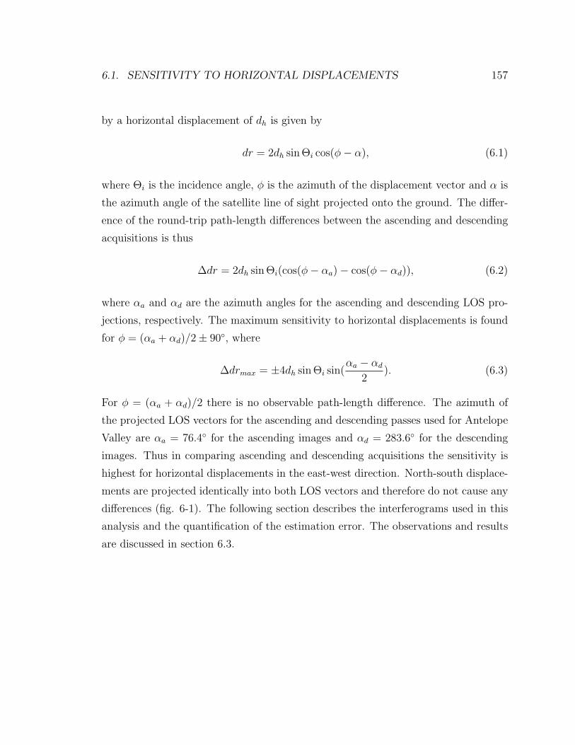
6.1. SENSITIVITY TO HORIZONTAL DISPLACEMENTS 157
by a horizontal displacement of dh is given by
dr = 2dh sin Θi cos(φ − α), (6.1)
where Θi is the incidence angle, φ is the azimuth of the displacement vector and α is
the azimuth angle of the satellite line of sight projected onto the ground. The differ-
ence of the round-trip path-length differences between the ascending and descending
acquisitions is thus
∆dr = 2dh sin Θi(cos(φ − αa) − cos(φ − αd)), (6.2)
where αa and αd are the azimuth angles for the ascending and descending LOS pro-
jections, respectively. The maximum sensitivity to horizontal displacements is found
for φ = (αa + αd)/2 ± 90◦, where
∆drmax = ±4dh sin Θi sin(αa − αd
2). (6.3)
For φ = (αa + αd)/2 there is no observable path-length difference. The azimuth of
the projected LOS vectors for the ascending and descending passes used for Antelope
Valley are αa = 76.4◦ for the ascending images and αd = 283.6◦ for the descending
images. Thus in comparing ascending and descending acquisitions the sensitivity is
highest for horizontal displacements in the east-west direction. North-south displace-
ments are projected identically into both LOS vectors and therefore do not cause any
differences (fig. 6-1). The following section describes the interferograms used in this
analysis and the quantification of the estimation error. The observations and results
are discussed in section 6.3.
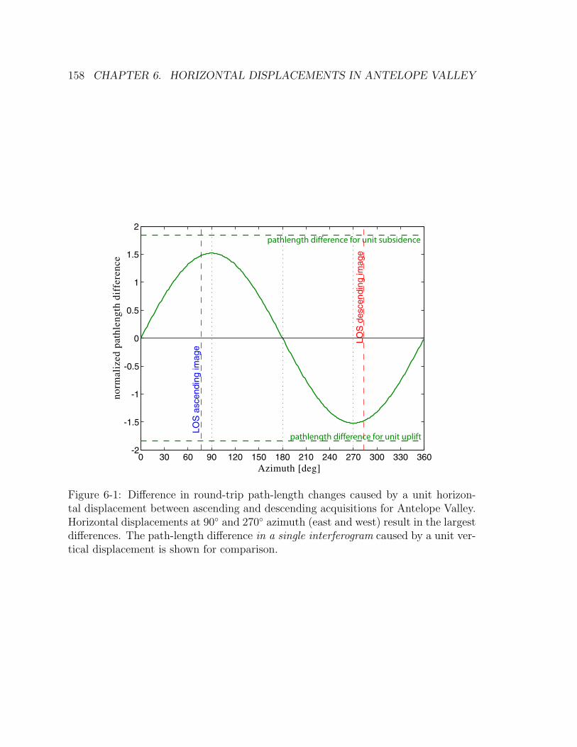
158 CHAPTER 6. HORIZONTAL DISPLACEMENTS IN ANTELOPE VALLEY
0 30 60 90 120 150 180 210 240 270 300 330 360-2
-1.5
-1
-0.5
0
0.5
1
1.5
2
LOS
asce
ndin
gim
age
LOS
desc
endi
ngim
age
Azimuth [deg]
norm
aliz
edpa
thle
ngth
diff
eren
ce
pathlength difference for unit uplift
pathlength difference for unit subsidence
Figure 6-1: Difference in round-trip path-length changes caused by a unit horizon-tal displacement between ascending and descending acquisitions for Antelope Valley.Horizontal displacements at 90◦ and 270◦ azimuth (east and west) result in the largestdifferences. The path-length difference in a single interferogram caused by a unit ver-tical displacement is shown for comparison.

6.2. DISPLACEMENT ESTIMATION 159
-1200
-1000
-800
-600
-400
-200
0
200
20148
23655
3982
19012
19513
20198
21200
23705
4032
5034
6036
7038
7539
9543
10545
11046
11547
15054
15555
19062
19563
1995 1996 1997 1998year
perp
endi
cula
rba
seli
ne[m
]
Figure 6-2: Ascending (blue) and descending (red) acquisitions and interferogramsused to estimate displacements. The pluses indicate acquisitions, labeled with theorbit number. The lines indicate the interferograms formed (see also tables 6.1 and6.2).
6.2 Displacement estimation
6.2.1 Available SAR acquisitions
One of the difficulties in the analysis presented in this chapter are the very specific
requirements for the acquired data. The ascending and descending acquisitions have
to span an identical or nearly identical time period. Furthermore, to derive inter-
ferometric displacement estimates from these acquisitions their temporal and spatial
(baseline) distribution must allow the formation of interferograms with sufficiently
high interferometric correlation (section 2.2.2). Most ERS SAR data over land areas
has been acquired on descending passes, while only relatively few ascending acquisi-
tions over land exist. This severely restricts the choice of data useful for the analysis
described here. Figure 6-2 shows the data used for both ascending and descending

160 CHAPTER 6. HORIZONTAL DISPLACEMENTS IN ANTELOPE VALLEY
Acquisition 1 Acquisition 2 Interferogramdate orbit σ2
a[rad2] date orbit σ2a[rad2] σ2
a[rad2]1999/01/13 19513 0.4716 1998/12/09 19012 0.4716 0.94311996/01/24 3982 0.3023 1998/12/09 19012 0.4716 1.81941998/12/09 19012 0.4716 1995/05/22 20148 0.2649 2.63521996/01/24 3982 0.3023 1996/01/22 23655 0.2649 0.66541996/01/24 3982 0.3023 1995/05/22 20148 0.2649 0.60471996/01/22 23655 0.2649 1995/05/22 20148 0.2649 0.5298
Table 6.1: Ascending interferograms used to study horizontal displacements. Theatmospheric variance estimates are given for the individual acquisitions and for theinterferograms. The variances for the individual acquisitions are used as covariancesfor interferograms sharing the acquisition.
satellite tracks. The blue and red lines indicate the interferograms formed using as-
cending and descending data, respectively (fig. 6-2), which are also listed in tables
6.1 and 6.2. Unfortunately, the ascending acquisition on January 13, 1999 (orbit
19513) and the descending acquisitions on May 26, 1995 (orbit 20198) and January
16, 1999 (orbit 19563) contain strong atmospheric delay signals. To derive the best
estimate of the surface displacements during May 1995 - January 1996, January 1996
- December 1998, and January 1996 to January 1999 for both ascending and descend-
ing imaging geometries, using the interferograms shown in figure 6-2, I employed a
variance-weighted least-squares estimation, described in the following paragraph.
6.2.2 Estimating displacements from several interferograms
Even if it were possible to form interferograms between the image acquisitions May
1995, January 1996, December 1998 and January 1999 for both ascending and de-
scending images, combining interferograms using intermediate image acquisitions may
result in more accurate displacement maps if shorter perpendicular baselines and/or
shorter time spans can be exploited to reduce the effects of spatial and temporal
decorrelation in the interferograms. For the available data presented in the previous
section, some of the perpendicular baselines between acquisitions spanning the above
time periods are excessively large, necessitating the combination of interferograms
with shorter baselines. This section describes a least-squares approach to obtain an

6.2. DISPLACEMENT ESTIMATION 161
Acquisition 1 Acquisition 2 Interferogramdate orbit σ2
a[rad2] date orbit σ2a[rad2] σ2
a[rad2]1999/01/16 19563 1.6309 1998/04/11 15555 0.8840 4.42791999/01/16 19563 1.6309 1997/07/05 11547 0.6095 3.61871999/01/16 19563 1.6309 1996/09/28 7539 0.1349 3.26181998/12/12 19062 1.1923 1998/03/07 15054 0.5685 2.38451998/12/12 19062 1.1923 1996/08/24 7038 0.5838 4.66501998/04/11 15555 0.8840 1998/03/07 15054 0.5685 3.38441998/04/11 15555 0.8840 1997/07/05 11547 0.6095 2.22331998/04/11 15555 0.8840 1997/05/31 11046 0.5955 1.76811998/04/11 15555 0.8840 1997/02/15 9543 0.2143 1.88341998/04/11 15555 0.8840 1996/09/28 7539 0.1349 2.07661998/03/07 15054 0.5685 1997/05/31 11046 0.5955 1.78681998/03/07 15054 0.5685 1997/04/26 10545 0.1526 1.13691997/07/05 11547 0.6095 1997/05/31 11046 0.5955 2.28331997/07/05 11547 0.6095 1997/02/15 9543 0.2143 1.70851997/07/05 11547 0.6095 1996/09/28 7539 0.1349 1.21901997/07/05 11547 0.6095 1996/06/15 6036 0.2742 1.60241997/07/05 11547 0.6095 1996/04/06 5034 0.1349 1.33381997/05/31 11046 0.5955 1997/02/15 9543 0.2143 1.52741997/05/31 11046 0.5955 1996/09/28 7539 0.1349 1.19111997/04/26 10545 0.1526 1997/02/15 9543 0.2143 0.52631997/04/26 10545 0.1526 1996/09/28 7539 0.1349 0.30521997/02/15 9543 0.2143 1996/09/28 7539 0.1349 0.42861997/02/15 9543 0.2143 1996/04/06 5034 0.1349 1.08681996/09/28 7539 0.1349 1996/06/15 6036 0.2742 0.54841996/09/28 7539 0.1349 1996/04/06 5034 0.1349 0.26981996/09/28 7539 0.1349 1996/01/26 23705 0.1820 1.15951996/08/24 7038 0.5838 1996/06/15 6036 0.2742 1.16761996/06/15 6036 0.2742 1996/04/06 5034 0.1349 2.62111996/04/06 5034 0.1349 1996/01/26 23705 0.1820 0.36391996/01/27 4032 0.3792 1996/01/26 23705 0.1820 0.75841996/01/27 4032 0.3792 1995/08/04 21200 1.7951 3.59011996/01/27 4032 0.3792 1995/05/26 20198 0.8669 3.65651996/01/26 23705 0.1820 1995/05/26 20198 0.8669 1.7338
Table 6.2: Descending interferograms used to study horizontal displacements. Theatmospheric variance estimates are given for the individual acquisitions and for theinterferograms. The variances for the individual acquisitions are used as covariancesfor interferograms sharing the acquisition.

162 CHAPTER 6. HORIZONTAL DISPLACEMENTS IN ANTELOPE VALLEY
optimal estimate of the displacements during any given time period spanned by the
acquisitions. A similar method has been applied by Usai [2001], who used a least-
squares scheme to merge several interferograms. The approach presented here differs
primarily in the variance weighting I applied to give more weight to measurements of
higher accuracy.
If di is the vector of displacement measurements at pixel i of all interferograms
mi is the vector of the displacements at that pixel location during the time periods
of interest, the problem can be written as
di = G mi, (6.4)
where G is a matrix containing zeros, ones and minus ones specifying the relation
between the data and the estimated model parameters. For example, for the ascending
data this is
d19513 19012
d3982 19012
d19012 20148
d3982 23655
d3982 20148
d23655 20148
=
1 −1 0
0 −1 0
0 1 1
0 0 0
0 0 1
0 0 1
d(Jan96 − Jan99)
d(Jan96 − Dec99)
d(May95 − Jan96)
, (6.5)
where I assumed that no deformation is occurring during the two days spanned by
the interferogram between orbit numbers 3982 and 23655. If Σdiis the data covari-
ance matrix containing an estimate of the variances and covariances at pixel i, the
displacements can be obtained from variance-weighted least squares:
mi = G−1g
di, with G−1g = (GTΣdi
−1G)−1GTΣdi
−1 (6.6)
and
Σmi= G−1
g ΣdiG−1T
g (6.7)

6.2. DISPLACEMENT ESTIMATION 163
as the estimation covariance matrix. The diagonal elements of Σmicontain the vari-
ances of the displacement estimates at location i.
A critical issue using this approach is the estimation of the covariance matrix Σdi
which varies as a function of image location. The two important processes affecting
error or uncertainty in the processed interferograms are the locally highly variable
image noise, which is mostly governed by the interferometric correlation, and signal
delays from a turbulent atmosphere that introduce an error signal into the measure-
ment (see section 2.2.2).
Spatial filtering in the image processing reduces the noise level in the final dis-
placement maps, but the accuracy of the final estimate depends on the variance of the
original, unfiltered estimate. This local variance has to be computed prior to phase
unwrapping, because images often cannot be successfully unwrapped without prior
filtering. I computed the variance of the wrapped phase locally on the sample of the
69 pixels within 4.5 pixels of each pixel location. The 2π-ambiguity was resolved by
assuming that all phase values are within π radians of the local mean phase value. For
larger variances this assumption biases the computed variance towards lower values.
Assuming that the unwrapped phase values are normally distributed, the variance
of their wrapped values can be computed (fig. 6-3). Using this relationship I deter-
mined the variance of a Gaussian distribution of the (unwrapped) phase values from
the variance computed on the wrapped values. The correction for small variances is
negligible (fig. 6-3). For larger variances the mapping becomes non-unique in the
presence of a noisy sample, as the measured variance approaches the theoretical value
for a uniformly distributed sample in [−π, π), 3.29 rad2. I considered variances of the
wrapped values exceeding a threshold variance of 2.8 to be infinite. These values in-
dicate completely decorrelated areas where the measured phase does not contain any
information on the displacement. Assigning a large variance to the observation re-
sults in zero weight in the estimation (eq. 6.6). Alternatively to computing the phase
statistics on the phase values themselves, they could be estimated from the image
correlation [Bamler and Just, 1993; Just and Bamler, 1994]. I chose to compute the
phase statistics on the actual phases though, as the relationship between correlation
and phase variance depends on the statistics of the scatterers in the image, which

164 CHAPTER 6. HORIZONTAL DISPLACEMENTS IN ANTELOPE VALLEY
0 1 2 2.8 3 4 5 60
0.5
1
1.5
2
2.5
3
3.28993.5
thre
shol
dva
lue
variance of unwrapped values [rad2]
vari
ance
ofw
rapp
edva
lues
[rad
2 ]
Figure 6-3: Relationship between the variances of unwrapped and wrapped phasevalues. Wrapped variances above the threshold value of 2.8 rad2 were assumed to beinfinite.
generally has to be assumed [Usai, 2001].
The variance due to noisy phase measurements is a property of the interfero-
metric phase difference and not the individual SAR acquisitions. It therefore does
not contribute to the covariances between interferograms. In contrast, atmospheric
delay signals are contained in individual SAR image acquisitions, even though they
only become noticeable in the interferometric phase differences. To estimate the vari-
ance of the atmospheric signal in each interferogram I computed the variance of the
unwrapped phase values in the area that was not known to deform. To limit the
contribution of small-scale noise to the variance, as this contribution was already ac-
counted for as described above, I computed the variance in the final, spatially filtered
images, using only pixels with correlation values exceeding 0.5. I assumed this “atmo-
spheric” variance to be spatially constant for each interferogram. Thus, the variance
for each image pixel was the sum of the spatially constant atmospheric variance and
the spatially variable variance due to decorrelation noise.
Because the atmospheric delay signal contained in any SAR acquisition will equally
affect all interferograms sharing this acquisition, the errors in these interferograms are

6.3. COMPARISON OF ASCENDING AND DESCENDING IMAGES 165
correlated. This must be accounted for in the off-diagonal elements of the data covari-
ance matrices Σdi. The covariance between two interferograms sharing an acquisition
with the atmospheric variance σ2a is either σ2
a, if the acquisition is master or slave in
both interferograms, or −σ2a, if the acquisition is the master image in one and the
slave image in the other interferogram. I used half the minimum variance found in all
interferograms sharing one particular acquisition as an estimate for the atmospheric
variance in this individual SAR acquisition. This guarantees that the sum of two
acquisition variances never exceeds the variance computed for an interferogram using
these two images. However, the highest variances will be underestimated while the
lowest variances will be overestimated. Tables 6.1 and 6.2 list the atmospheric vari-
ances for all interferograms shown in figure 6-2 and the estimates for the individual
acquisitions. Using the spatially variable covariance matrices in equation 6.6 resulted
in the displacement estimates shown and discussed in the following section.
6.3 Comparison of ascending and descending im-
ages
The estimated vertical subsidence derived from ascending and descending acquisitions
for the time periods January 1996 to December 1998 and January 1996 to January
1999 agree very closely (fig. 6-4), both in magnitude and the detailed structure of
the observed subsidence. In agreement with the observations presented in section 4.2,
the two main subsidence features are the subsidence bowl in Lancaster and a smaller
area south of Rogers Lake. Due to strong atmospheric delay signals in the descending
acquisitions in January 1999 (orbit 19563) and May 1995 (orbit 20198), the corre-
sponding images show strong atmospheric noise signals (fig. 6-4, top and bottom
right), making a straightforward visual comparison of the ascending and descending
images difficult. To visualize more subtle differences in the area of the Lancaster
subsidence bowl (yellow frame in fig. 6-4) the displacement maps are also displayed
with a wrapped colormap (fig. 6-5). Although this representation results in a much
noisier appearance, the visible differences appear to be related to atmospheric effects,

166 CHAPTER 6. HORIZONTAL DISPLACEMENTS IN ANTELOPE VALLEY
Ascending
May
1995
-Ja
n.19
96
-5
0
5
10
15
20
25
30Descending
Jan.
1996
-D
ec.1
998
-20
0
20
40
60
80
Jan.
1996
-Ja
n.19
99
-20
0
20
40
60
80
millim
etersm
illimeters
millim
eters
10 km
CALIFORNIA
14
CALIFORNIA
58
CALIFORNIA
381
10 km
CALIFORNIA
14
CALIFORNIA
58
CALIFORNIA
381
10 km
CALIFORNIA
14
CALIFORNIA
58
CALIFORNIA
381
10 km
CALIFORNIA
14
CALIFORNIA
58
CALIFORNIA
381
10 km
CALIFORNIA
14
CALIFORNIA
58
CALIFORNIA
381
10 km
CALIFORNIA
14
CALIFORNIA
58
CALIFORNIA
381
Profile A Profile A
Profile A Profile A
-118 10' -118 00' -117 50' -118 10' -118 00' -117 50' -117 40'
LOS LOS
LOS LOS
LOS LOS
Figure 6-4: Comparison of displacement maps derived from ascending and descendingobservations for three time period. The values are shown in terms of equivalent ver-tical displacement assuming no horizontal displacement. The yellow frame indicatesthe area shown in figures 6-5, 6-6 and 6-7.

6.3. COMPARISON OF ASCENDING AND DESCENDING IMAGES 167
not horizontal displacement. The most apparent spatially coherent difference is the
fringe spacing on the southern side of the subsidence bowl in the three-year images.
The fringes are further apart in the descending image than in the ascending image
(fig. 6-5). However, horizontal displacements in this area are expected to be directed
to the north, and consequently not appear differently in these images (see fig. 6-1).
It is therefore more likely that this difference is also of atmospheric origin. Although
differences in the ascending and descending images in many locations exceed one or
even two centimeters (fig. 6-6, 6-8, 6-9, 6-10), the spatial patterns of these differences
do not appear to be correlated with the subsidence bowl. Their spatial distribution
strongly suggests atmospheric delays as their origin. Furthermore, in most areas the
differences are within one standard deviation of the difference estimate (fig. 6-6,
6-7). The significance of the difference between the vertical displacement estimates
can be tested using a statistical T-test [Davis, 1986]. Figure 6-7 shows the differ-
ence between the ascending and descending displacement estimate normalized by the
standard deviation (the t-value) and the locations where the vertical displacement
estimates are different at a 5% significance level. The result indicates that the obser-
vations from the two orbital tracks are not significantly different given the variance
of the estimates. The displacements along the profiles indicated in figures 6-4 and
6-5 are shown in figures 6-8, 6-9 and 6-10. Again, although differences of one or
two centimeters equivalent vertical displacements are not uncommon, they are not
correlated with the sides of the subsidence bowl, where horizontal displacements are
expected to be greatest. The relatively large differences during January 1996 to De-
cember 1998 along the first six kilometers of profile C (fig. 6-10) are unlikely to be
due to horizontal displacements, because of the unfavorable expected orientation of
horizontal displacements (fig. 6-1) and the absence of these differences in the January
1996 to January 1999 observations.
While the displacement maps derived from ascending and descending observa-
tions are not significantly different given the variances of the displacement estimates,
it should be pointed out that horizontal displacements of more than a centimeter may
occur even in the east-west direction, where the difference measurement is most sen-
sitive to these displacements, without being reliably detected. For displacements at

168 CHAPTER 6. HORIZONTAL DISPLACEMENTS IN ANTELOPE VALLEY
AscendingM
ay19
95-
Jan.
1996
DescendingJa
n.19
96-
Dec
.199
8Ja
n.19
96-
Jan.
1999
-118 10' -118 06' -118 02'
5 km
ProfileBP
rofileC
-118 10' -118 06' -118 02'
5 km
ProfileBP
rofileC
5 km
ProfileBP
rofileC
5 km
ProfileBP
rofileC
5 km5 km
0 10
5
-5
Upl
ift
Subsidence
verticalmillimeters
LOS LOS
LOS LOS
LOS LOS
Figure 6-5: Comparison of displacements in area indicated by yellow frame in figure6-4. The values are shown using a wrapped colorscale to enhance the visibility ofsmall-scale features. Also, the descending values were adjusted by up to 5mm tomake the color patterns more easily comparable by eye.

6.3. COMPARISON OF ASCENDING AND DESCENDING IMAGES 169
Difference
May
1995
-Ja
n.19
96
0
5
10
15
20Std. Deviation
Jan.
1996
-D
ec.1
998
0
5
10
15
20
Jan.
1996
-Ja
n.19
99
0
5
10
15
20
millim
etersm
illimeters
millim
eters
-118 10' -118 06' -118 02'
5 km
-118 10' -118 06' -118 02'
5 km
5 km5 km
5 km5 km
LOS LOS
LOS LOS
LOS LOS
Figure 6-6: Absolute difference between displacement maps derived from ascendingand descending acquisitions. The patterns suggest an atmospheric process causingthese differences. For large areas the difference is smaller than one standard deviationof the estimates (see also fig. 6-7).

170 CHAPTER 6. HORIZONTAL DISPLACEMENTS IN ANTELOPE VALLEY
-2
-1
0
1
2Difference / σ
May
1995
-Ja
n.19
96
-2
-1
0
1
2
Jan.
1996
-D
ec.1
998
-2
-1
0
1
2
Jan.
1996
-Ja
n.19
99
different at 95% confidence?
-118 10' -118 06' -118 02'
5 km
-118 10' -118 06' -118 02'
5 km
5 km5 km
5 km5 km
Figure 6-7: Left: Differences between displacement maps from ascending and de-scending acquisitions normalized by the standard deviation. For most locations thedifference is below one standard deviation. Right: Result of a T-test testing thehypothesis if the values from ascending and descending images are different at a 5%significance level. In the white areas the hypothesis cannot be accepted. The few lo-cations where the hypothesis is accepted (black dots) do not appear to be correlatedwith the subsidence bowl.

6.3. COMPARISON OF ASCENDING AND DESCENDING IMAGES 171
0 5 10 15 20 25 30 35 40 45 50
-40
-20
0
20
40
60
80
Jan. 1996 - Dec. 1998, Profile A
vert
.sub
side
nce
[mm
]
-40
-20
0
20
40
min.horiz.displacem
ent[mm
]
-40
-30
-20
-10
0
10
20
30
40
asc
min
usde
sc[v
ert.
mm
]
0 5 10 15 20 25 30 35 40 45 50distance along profiff le A [km]
DescendingAscending
W E
W E
0 5 10 15 20 25 30 35 40 45 50
-40
-20
0
20
40
60
80
Jan. 1996 - Jan. 1999, Profile A
vert
.sub
side
nce
[mm
]
-40
-20
0
20
40
min.horiz.displacem
ent[mm
]
-40
-30
-20
-10
0
10
20
30
40
asc
min
usde
sc[v
ert.
mm
]
0 5 10 15 20 25 30 35 40 45 50distance along profile A [km]
DescendingAscending
W E
W E
Figure 6-8: Comparison of displacements from ascending and descending acquisitionsalong profile A (fig. 6-4). The shaded areas around the lines indicate 1-σ errorbars. The right ordinate on the bottom indicates the equivalent optimally orientedhorizontal displacement.

172 CHAPTER 6. HORIZONTAL DISPLACEMENTS IN ANTELOPE VALLEY
0 2 4 6 8 10 12 14 16
-40
-20
0
20
40
60
80
Jan. 1996 - Dec. 1998, Profile Bve
rt.s
ubsi
denc
e[m
m]
-40
-20
0
20
40
min.horiz.displacem
ent[mm
]-40
-30
-20
-10
0
10
20
30
40
asc
min
usde
sc[v
ert.
mm
]
0 2 4 6 8 10 12 14 16distance along profile B [km]
DescendingAscending
SW NE
SW NE
0 2 4 6 8 10 12 14 16
-40
-20
0
20
40
60
80
Jan. 1996 - Jan. 1999, Profile B
vert
.sub
side
nce
[mm
]
-40
-20
0
20
40
min.horiz.displacem
ent[mm
]-40
-30
-20
-10
0
10
20
30
40
asc
min
usde
sc[v
ert.
mm
]
0 2 4 6 8 10 12 14 16distance along profile B [km]
DescendingAscending
SW NE
SW NE
Figure 6-9: Comparison of displacements from ascending and descending acquisitionsalong profile B (fig. 6-5). The shaded areas around the lines indicate 1-σ errorbars. The right ordinate on the bottom indicates the equivalent optimally orientedhorizontal displacement.

6.3. COMPARISON OF ASCENDING AND DESCENDING IMAGES 173
0 1 2 3 4 5 6 7 8 9
-40
-20
0
20
40
60
80
Jan. 1996 - Dec. 1998, Profile C
vert
.sub
side
nce
[mm
]
-40
-20
0
20
40
min.horiz.displacem
ent[mm
]-40
-30
-20
-10
0
10
20
30
40
asc
min
usde
sc[v
ert.
mm
]
0 1 2 3 4 5 6 7 8 9distance along profile C [km]
DescendingAscending
S N
S N
0 1 2 3 4 5 6 7 8 9
-40
-20
0
20
40
60
80
Jan. 1996 - Jan. 1999, Profile C
vert
.sub
side
nce
[mm
]
-40
-20
0
20
40
min.horiz.displacem
ent[mm
]-40
-30
-20
-10
0
10
20
30
40
asc
min
usde
sc[v
ert.
mm
]
0 1 2 3 4 5 6 7 8 9distance along profile C [km]
DescendingAscending
S N
S N
Figure 6-10: Comparison of displacements from ascending and descending acquisitionsalong profile C (fig. 6-5). The shaded areas around the lines indicate 1-σ errorbars. The right ordinate on the bottom indicates the equivalent optimally orientedhorizontal displacement.

174 CHAPTER 6. HORIZONTAL DISPLACEMENTS IN ANTELOPE VALLEY
larger angles to this direction, even much larger displacements may not be detectable
at the level of statistical significance. However, notwithstanding the relatively large
uncertainty of the absolute difference values, the absence of differences that are spa-
tially correlated with the subsidence bowl does in fact support the hypothesis that
horizontal surface displacements accompanying inelastic aquifer system compaction
are small and probably negligible. This may not be true for elastic displacements such
as those observed by Bawden et al. [2001], which occur primarily in the aquifers. Un-
fortunately, the lack of more ascending SAR acquisitions prevented an investigation
of horizontal displacements in connection to seasonal elastic deformation in Antelope
Valley here.

Chapter 7
Conclusions
This chapter summarizes my general conclusions from the work presented in the
previous chapters. Detailed conclusions for the individual case studies have already
been presented in the respective chapters. In this chapter I focus on conclusions
pertaining to the general questions and problems I set out to address in Chapter 1
(p. 5), placing this work in the larger context of applying InSAR technology to the
study of aquifer systems.
7.1 Results and implications
I have found InSAR techniques to be well suited to measure and monitor ground
surface displacements over the two aquifer systems studied. The dry and bare or ur-
banized land surfaces permitted forming interferograms spanning several years with-
out prohibitive loss of signal due to decorrelation. The achievable accuracies were
generally on the order of 1 cm or less and the spatial resolution was significantly
higher than the spatial resolution of any other data, such as the hydraulic head or
material properties, available for these aquifer systems. Beyond simply studying sur-
face deformation itself, any analysis requiring conjunctive interpretation of different
data is therefore no longer restricted by the paucity of surface displacement data,
but by the scarcity of other data. For example, the estimation of spatially variable
elastic (Chapter 3) or inelastic (Chapter 4) skeletal storage coefficients was limited
by the lack of more detailed and more reliable knowledge of the hydraulic heads in
the aquifer system.
175

176 CHAPTER 7. CONCLUSIONS
The accuracy of InSAR-derived displacement maps for the aquifer systems studied
proved to be limited primarily by the presence of atmospheric phase signals in the
interferograms. The measurement error for detailed interpretations of these displace-
ments therefore depends on the ability to remove or at least reliably identify these
atmospheric signals. Furthermore, deviations of the displacement from the assumed
(vertical) direction can bias the displacement estimates. However, investigating dis-
placement maps derived from acquisitions on different satellite tracks I did not find
an indication of significant horizontal displacements related to several centimeters of
subsidence in Antelope Valley. This indicates that horizontal surface displacements
may be negligible for inelastic aquifer system compaction at the regional scale.
I have found that displacement observations over long time periods were necessary
to constrain estimations of the compaction time constants in Antelope Valley (Chap-
ter 4). Although the available catalog for ERS SAR data now contains acquisitions
over the past 10 years this remains insufficient to constrain the estimation of time
constants on the order of decades to centuries. Thus, the newness of the technique
and the correspondingly limited amount of available historical data currently restricts
the usefulness of InSAR in the interpretation of delayed deformation processes.
The very high spatial resolution of ERS SAR imagery permits the observation of
the surface deformation patterns with great spatial detail. This can be extremely
useful in determining the exact location of structural boundaries, such as faults,
sudden changes in subsurface composition or sediment thickness, provided that stress
changes induce differential displacements to highlight these boundaries.
One of the most important observational advances using InSAR is the ability to
characterize the time-variability of the deformation process at much higher temporal
resolution than previously possible using geodetic observations from benchmark sur-
veys or campaign GPS. The 35 day orbit repeat cycle of the ERS satellites enables
the detection of displacement transients down to almost monthly time-scales. Even
though not every acquisition may be usable for conventional InSAR in practice, due to
excessively long perpendicular baselines or strong atmospheric artifacts, the temporal
frequency of observations exceeds that of most other techniques available today. If an
even higher observation frequency is required, observations from different sensors or

7.1. RESULTS AND IMPLICATIONS 177
satellite tracks might be used. In both aquifer systems studied I observed temporal
variability of the displacement field at the shortest observable time scales. Long-term
displacement trends were usually superposed with a seasonally fluctuating signal. In
some locations even shorter transients are observable. These are probably caused by
local pumping operations. Both seasonal and transient displacement signals are an
important aspect of the displacement field and can be analyzed in terms of aquifer
system properties, such as the elastic storage coefficients. Seasonal and transient
surface displacements over aquifer systems have not received much attention prior to
this work, primarily due to the lack of adequate observations. Chapter 3 constitutes
the first detailed investigation of seasonal displacement signals over an aquifer system
and the first estimation of spatially variable elastic aquifer system storage coefficients
from InSAR data. The subsidence observed over the Antelope Valley aquifer system
(Chapter 4) can also not be described by a constant subsidence rate. Any attempt
to interpret the surface displacements in terms of the underlying physical process
must adequately account for the true complexity of the subsidence signal. However,
it seems to be possible to neglect seasonal fluctuations of both pore pressures and
surface subsidence in the estimation of inelastic skeletal storage coefficients.
I have shown how the elastic skeletal storage coefficient of the aquifer system, the
inelastic skeletal storage coefficient of interbeds and compaction time constants can
be estimated from surface displacement observations and known changes of hydraulic
head in a confined aquifer system. I have further demonstrated for the first time
that these parameters can be estimated for many locations across an aquifer system
if both subsidence and head change observations are available for an extended area.
However, while the subsidence observations derived from InSAR yielded sufficiently
accurate and detailed measurements of the surface displacements, the reliability of
the estimated parameters was impaired by inaccurate or unreliable estimates of the
stress changes in the aquifer systems and biased by conceptual misrepresentations
of the aquifer system. Smaller study sites with densely spaced observation wells
and detailed data on the geometry of the hydrogeologic units would provide a more
controlled experiment, enabling more reliable parameter estimations. Particularly in
site-scale studies, however, one-dimensional observations of surface displacement may

178 CHAPTER 7. CONCLUSIONS
not suffice to characterize the surface displacements adequately, necessitating more
realistic models for the mechanical behavior of the subsurface materials.
7.2 Future research and applications
The application of InSAR to studies of developed aquifer systems is still in its infancy.
Developments of the processing tools will make these data more easily accessible to
a larger community of scientists and engineers. The advanced capability of measur-
ing surface displacements will allow them to develop and constrain more complex
geomechanical models of the aquifer systems. Parallel advances in the tools for nu-
merical simulation will enable the development of sophisticated geomechanical models
of developed aquifer systems, providing a powerful tool for optimizing groundwater
pumping with respect to land subsidence problems.
Routine InSAR mapping can play an important role in siting structures that
are particularly sensitive to ground displacements such as the routing of pipelines
or aqueducts over terrain susceptible to deformation. Where such infrastructure is
already in place, InSAR-derived deformation maps can be used to assess the risk of
breakage and identify most vulnerable locations.
In this work I have used the available subsidence data in conjunction with observed
or simulated changes in hydraulic head to estimate storage coefficients and compaction
time constants. Where additional information on the aquifer system is available it
may be possible to estimate additional parameters from these data. If the geometry
of the aquifer system, in particular the thicknesses of compacting layers, is known
accurately, the vertical diffusivity of the compacting interbeds can be determined from
the compaction time constants. In relatively simple, elastically deforming aquifer
systems it should also be feasible to estimate changes in subsurface pore pressure
(i.e. hydraulic head) from surface displacement observations, after the parameters
governing the elastic deformation process have been calibrated. This would provide
a uniquely powerful tool to monitor changes in hydraulic head at the unprecedented
detail of SAR images. Such an approach would also be a valuable supplement to
gravity studies to monitor changes in basin-wide water storage, such as the GRACE

7.3. CLOSING REMARKS 179
satellite mission [Rodell and Famiglietti, 1999].
The applicability of InSAR techniques is severely curtailed in densely vegetated
areas due to the loss of signal by decorrelation. This problem may be at least partly
overcome by future sensors operating at longer radar wavelengths, which are not as
strongly affected by vegetation. Also, recent developments indicate that interfer-
ometry can be performed on a sparse grid of highly coherent individual scatterers
(“permanent scatterer”), vastly extending the applicability of InSAR in vegetated
areas.
Finally, InSAR data acquired over aquifer systems can be useful beyond the mea-
surement of deformation. Some studies have attempted to relate interferometric phase
signatures to soil moisture [Fatland and Nolan, 2001]. Furthermore, a largely un-
tapped opportunity is the use of InSAR correlation maps as a mapping tool for
change detection. These maps might be used for surface classification or verification
of land fallowing agreements, for example.
7.3 Closing remarks
Where the technique is applicable, InSAR is rapidly developing into an indispensable
tool for monitoring ongoing surface displacements over deforming aquifer systems.
The surface displacement observations provide an additional constraint in calibrating
groundwater flow and subsidence models. With observational data for their calibra-
tion available, deformation processes are likely to be routinely included in numerical
models, particularly where land subsidence is a concern in groundwater management
decisions. On the previous 179 pages I have demonstrated some of the analyses en-
abled by the wealth of surface displacement data available from InSAR. Hopefully
my results will encourage future applications and research, using one of todays most
sophisticated space-borne imaging technologies to study one of our most vital and
valuable resources: water.

180 CHAPTER 7. CONCLUSIONS

Appendix A
Details of the Antelope Valley
groundwater flow model
This appendix contains detailed information on the groundwater flow and subsidence
model used for the simulation and parameter inversion described in Chapter 4. The
model was developed by Leighton and Phillips [2003], who provided me with their
input files. I refer to their model as “the original model” herein. I modified this
original model in the following three aspects:
1. The original model was based on MODFLOW-88 [McDonald and Harbaugh,
1988]. I changed the original input files to run my simulations using MODFLOW-
96 [Harbaugh and McDonald, 1996]. This represents a minor change and only
affected the format of some of the input file, but not the computations performed
in the simulation or the simulation results.
2. The original model used annual stress periods for the time period from 1915
through 1995. Using more recent pumping data for the years 1996 to 1998 (Steve
Phillips, U.S. Geological Survey, written comm.) I extended the simulated time
period to the end of 1998.
3. The original model used the interbed storage package (IBS1) [Leake and Prudic,
1991] to simulate aquifer system compaction and land subsidence. For my
simulations I used the IBS2 package, developed by Leake [1990]. The calibration
of the required input parameters for this package is the topic of Chapter 4.
181

182 APPENDIX A. ANTELOPE VALLEY GROUNDWATER FLOW MODEL
G ar lo ckF au ltZ on e
ET-area
-118 30' -118 15' -118 00' -117 45'
34 45'
35 00'
30 km
Lancaster
Palmdale
Rosamond
EAFB
Roadsubbasin boundaryfault zone
34 30'
CALIFORNIA
58CALIFORNIA
14
CALIFORNIA
381
CALIFORNIA
14
S a nA n d r e a s
F a u l t Z o n e
Figure A-1: Area covered by model grid. Shown are only the active cells in the modellayers. Black cells are active (IBOUND value 1) in all three model layers. The darkgray cells are only active in the top and middle layers and the light gray cells areonly active in the top layer. All active cells in the model are variable head cells.All boundaries are no-flow boundaries. Any inflow and outflow across the modelboundaries is simulated through wells in the boundary cells. The cells for whichevapotranspiration is simulated are indicated by the yellow frame.
The development and calibration of the original model to aquifer heads at 19 wells and
subsidence at 10 benchmark locations is reported in detail by Leighton and Phillips
[2003]. Rather than mirroring their work here, I will merely present the resulting
groundwater flow model (including my modifications).
A.1 Model grid
The model uses a regular finite difference grid with 43 rows (east-west), 60 columns
(north-south) and three model layers. Each model cell extends 1 by 1 mile horizon-
tally. The thicknesses of the model cells vary spatially. The total area covered by this
model grid is shown in figure A-1. Groundwater flow is only simulated for a subset of
the cells. The active cells for the three model layers are defined by the MODFLOW

A.2. FLOW PROPERTIES 183
IBOUND arrays (fig. A-1). All active cells in the model are variable head cells. All
model boundaries are no-flow boundaries.
A.2 Flow properties
A.2.1 Horizontal groundwater flow
The model uses the block-centered flow package (BCF) [McDonald and Harbaugh,
1988] for the groundwater flow computations. The upper model layer is identified
as confined/unconfined and the middle and lower layers are specified as confined.
The BCF package requires different input parameters for these two cases. For the
confined/unconfined (top) layer the horizontal hydraulic conductivity needs to be
specified (fig. A-2). The transmissivity is then computed by the package as the
product of the hydraulic conductivity and the saturated thickness in the layer. For
confined layers the saturated thickness does not change during the simulation. The
BCF package requires the transmissivity to be specified directly for these layers (fig.
A-2).
Several faults in the Antelope Valley aquifer system are represented in the model
using the horizontal flow barrier (HFB) package [Hsieh and Freckleton, 1992]. The
faults (fig. A-2) are assigned a “hydraulic characteristic”, defined as the hydraulic
conductivity or transmissivity (for unconfined/confined and confined layers, respec-
tively) divided by the width of the fault zone (or, more generally, horizontal-flow
barrier) [Hsieh and Freckleton, 1992]. The values used for the different faults are
indicated in figure A-2.
A.2.2 Vertical groundwater flow
The BCF package parameterizes the vertical flow properties by using a quantity called
the “vertical leakance” [McDonald and Harbaugh, 1988] instead of using a vertical
hydraulic conductivity, Kv and the layer thickness, z. The vertical leakance is defined

184 APPENDIX A. ANTELOPE VALLEY GROUNDWATER FLOW MODEL
S a nA n d r e a s
F a u l t Z o n e
G ar lo ckF au ltZ on e
S a nA n d r e a s
F a u l t Z o n e
G ar lo ckF au ltZ on e
S a nA n d r e a s
F a u l t Z o n e
G ar lo ckF au ltZ on e
Layer 1
Layer 2
Layer 3
0
2
4
6
8
0
100
200
300
400
500
0
20
40
60
80
100
Transm
issivity[m
2/day]T
ransmissivity
[m2/day]
Conductivity
[m/day]
30 km
30 km
30 km
CALIFORNIA
58CALIFORNIA
14
CALIFORNIA
381
CALIFORNIA
14
CALIFORNIA
58CALIFORNIA
14
CALIFORNIA
381
CALIFORNIA
14
CALIFORNIA
58CALIFORNIA
14
CALIFORNIA
381
CALIFORNIA
14
10-5
10-5
10-3
10-3
10-4
3x10⁻⁴
4x10⁻⁴
4x10⁻³
2x10⁻³
8x10⁻⁴
2x10⁻⁵
7x10⁻⁵
8x10⁻⁵
10-4
10-2
10-2
10-34x10-2
2x10⁻²
8x10⁻³
2x10⁻⁴
7x10-48x10-4
10-2
10-2
10-3
4x10⁻²
2x10⁻²
8x10⁻³
2x10⁻⁴
7x10-48x10-4
Figure A-2: Horizontal hydraulic conductivity (layer 1) and transmissivity (layers 2and 3) in the model. A number of horizontal-flow barriers (using the HFB package)are also specified (white lines). The “hydraulic characteristic” (see text) in day−1 isindicated for each flow barrier by the white numbers.

A.2. FLOW PROPERTIES 185
S a nA n d r e a s
F a u l t Z o n e
G ar lo ckF au ltZ on e
S a nA n d r e a s
F a u l t Z o n e
G ar lo ckF au ltZ on e
Layer 1/Layer 2
Layer 2/Layer 3
0
200
400
600
800
0
20
40
60
80
100
vert.leakance[10
-6day
-1]vert.leakance
[10-6
day-1]
30 km
Lancaster
Palmdale
Rosamond
EAFB
30 km
Lancaster
Palmdale
Rosamond
EAFB
CALIFORNIA
58CALIFORNIA
14
CALIFORNIA
381
CALIFORNIA
14
CALIFORNIA
58CALIFORNIA
14
CALIFORNIA
381
CALIFORNIA
14
Figure A-3: Vertical leakance between layers 1 and 2 and layers 2 and 3.

186 APPENDIX A. ANTELOPE VALLEY GROUNDWATER FLOW MODEL
S a nA n d r e a s
F a u l t Z o n e
G ar lo ckF au ltZ on e
Layer 10
0.05
0.1
0.12
0.14
specificyield
30 km
Lancaster
Palmdale
Rosamond
EAFB
CALIFORNIA
58CALIFORNIA
14
CALIFORNIA
381
CALIFORNIA
14
Figure A-4: Specific yield specified for layer 1. The value is used for cells in whichthe aquifer is not fully saturated during a stress periods. For saturated (confined)conditions the storage coefficient (fig. A-5) is used.
as [McDonald and Harbaugh, 1988]
VCONTk+1/2 =1
zk
2(Kv)k+ zk+1
2(Kv)k+1
, (A.1)
where VCONTk+1/2 is the vertical leakance between layers k and k + 1, zk and zk+1 are
the local layer thicknesses and the Kv are the local vertical hydraulic conductivities
for layers k and k + 1. These vertical leakance values specified between the top and
middle layers and the middle and bottom layers are shown in figure A-3.
A.2.3 Storage
Storage in the aquifer system is simulated in two separate packages. The BCF package
accounts for storage in the aquifers. Storage and storage changes in confining units
and interbeds are accounted for in the interbed storage package (IBS2) or subsidence
package (SUB). This is discussed in detail in section 4.3.2.

A.2. FLOW PROPERTIES 187
S a nA n d r e a s
F a u l t Z o n e
G ar lo ckF au ltZ on e
S a nA n d r e a s
F a u l t Z o n e
G ar lo ckF au ltZ on e
S a nA n d r e a s
F a u l t Z o n e
G ar lo ckF au ltZ on e
Layer 1
Layer 2
Layer 3
0
1
2
3
4
5
0
0.5
1
1.5
0
2
4
6
8
10
storagecoefficient[10
-4]storage
coefficient[10-4]
storagecoefficient[10
-4]
30 km
Lancaster
Palmdale
Rosamond
EAFB
30 km
Lancaster
Palmdale
Rosamond
EAFB
30 km
Lancaster
Palmdale
Rosamond
EAFB
CALIFORNIA
58CALIFORNIA
14
CALIFORNIA
381
CALIFORNIA
14
CALIFORNIA
58CALIFORNIA
14
CALIFORNIA
381
CALIFORNIA
14
CALIFORNIA
58CALIFORNIA
14
CALIFORNIA
381
CALIFORNIA
14
Figure A-5: Primary aquifer storage coefficients specified in the model. For cells thatbecome unsaturated (only in the upper layer), the specific yield is used instead (fig.A-4).

188 APPENDIX A. ANTELOPE VALLEY GROUNDWATER FLOW MODEL
Aquifer storage
The BCF package requires a dimensionless storage coefficient to be specified for each
model layer. This is the storage coefficient (eq. 2.10) for the confined layers (layers
2 and 3, fig. A-5) and the specific yield for the unconfined layers. For the top layer,
which is specified as confined/unconfined, both values are provided as input to the
package (figs. A-4 and A-5).
Interbed storage
As I discussed in detail in section 4.3.2, the IBS2 package [Hoffmann et al., 2003b]
uses two different parameterizations for storage in interbeds. For interbeds in which
the hydraulic heads are assumed to equilibrate with the heads in the aquifers instan-
taneously two storage coefficients, Ske and Skv, for elastic and inelastic deformation,
respectively, must be specified (figs. A-6 and A-7). For interbeds in which the heads
can equilibrate only very slowly with the changing heads in the surrounding aquifers
and elastic and inelastic specific storage (Sske and Sskv, respectively) and their ver-
tical hydraulic conductivity, Kv, are specified for the interbeds. In the model these
values were constant over the entire model domain (table 4.5). The storage in these
interbeds is then computed using the other input parameters, namely the equivalent
thickness, beq, and the number of individual interbeds, N (table 4.3). In the model
interbed storage is only assigned to the upper two model layers. Only the middle
model layer (layer 2) is assigned interbeds with delay properties. The elastic and
inelastic storages are set to identical values for each of the two layers (i.e., the in-
elastic storage for interbeds in the top layer is equal to the elastic storage; similarly
for the middle layer). Thus, all inelastic interbed storage is simulated in interbeds
with delay properties in layer 2. The elastic and inelastic storage, and the initial
preconsolidation head for interbeds without delay properties in the upper two layers
are shown in figures A-6 and A-7. The values for beq and N in the middle model layer
are shown in figure A-8. The initial preconsolidation head for the delayed interbeds
in that layer is uniformly 1.2m below the starting head in that layer (fig. A-11).

A.2. FLOW PROPERTIES 189
S a nA n d r e a s
F a u l t Z o n e
G ar lo ckF au ltZ on e
S a nA n d r e a s
F a u l t Z o n e
G ar lo ckF au ltZ on e
Layer 1
Layer 1
0
5
10
15
20
700
750
800
850
900
950 preconsolidationhead
[ma.s.l.]
elasticand
inelasticinterbed
storagecoefficient[10
-4]30 km
Lancaster
Palmdale
Rosamond
EAFB
30 km
Lancaster
Palmdale
Rosamond
EAFB
CALIFORNIA
58CALIFORNIA
14
CALIFORNIA
381
CALIFORNIA
14
CALIFORNIA
58CALIFORNIA
14
CALIFORNIA
381
CALIFORNIA
14
Figure A-6: Elastic and inelastic storage and the initial preconsolidation head for theupper model layer. The values for inelastic and elastic instantaneous interbeds wereequal as inelastic compaction was simulated only for interbeds with delay propertiesin layer 2 (section 4.3.2). The properties of these interbeds are shown in figure A-8.

190 APPENDIX A. ANTELOPE VALLEY GROUNDWATER FLOW MODEL
S a nA n d r e a s
F a u l t Z o n e
G ar lo ckF au ltZ on e
S a nA n d r e a s
F a u l t Z o n e
G ar lo ckF au ltZ on e
Layer 2
Layer 2
0
1
2
3
4
5
6
700
750
800
850
900 preconsolidationhead
[ma.s.l.]
elasticand
inelasticinterbed
storagecoefficient[10
-4]30 km
Lancaster
Palmdale
Rosamond
EAFB
30 km
Lancaster
Palmdale
Rosamond
EAFB
CALIFORNIA
58CALIFORNIA
14
CALIFORNIA
381
CALIFORNIA
14
CALIFORNIA
58CALIFORNIA
14
CALIFORNIA
381
CALIFORNIA
14
Figure A-7: Elastic and inelastic storage and the initial preconsolidation head for themiddle model layer. Interbeds with delay properties require additional parameters(fig. A-8). By setting the inelastic storage of interbeds without delay propertiesequal to the elastic storage all inelastic compaction is simulated in interbeds withdelay properties.

A.2. FLOW PROPERTIES 191
S a nA n d r e a s
F a u l t Z o n e
G ar lo ckF au ltZ on e
S a nA n d r e a s
F a u l t Z o n e
G ar lo ckF au ltZ on e
Layer 2
Layer 2
0
10
20
30
1
2
3
4
5
beq
[m]
number
ofinterbeds
30 km
Lancaster
Palmdale
Rosamond
EAFB
30 km
Lancaster
Palmdale
Rosamond
EAFB
CALIFORNIA
58CALIFORNIA
14
CALIFORNIA
381
CALIFORNIA
14
CALIFORNIA
58CALIFORNIA
14
CALIFORNIA
381
CALIFORNIA
14
Figure A-8: Equivalent interbed thickness (beq, see eq. 2.14) and the number ofindividual interbeds, N for interbeds with delay properties in the middle model layer.The resulting total inelastic storage coefficients and time constants are shown in figure4-13.

192 APPENDIX A. ANTELOPE VALLEY GROUNDWATER FLOW MODEL
A.3 In- and outflow
Because only variable-head cells are used in the model, all outer model boundaries
represent no-flow boundaries. Water enters the model domain as recharge (using the
recharge (RCH) package) or through wells (using the well (WEL) package) [McDonald
and Harbaugh, 1988]. Water leaves the model via evapotranspiration (ET), negative
recharge (simulating outflow), or pumping wells.
A.3.1 Evapotranspiration
The area for which evapotranspiration is considered is indicated by the yellow frame
in figure A-1. The ET flux in this area depends on the depth of the water table below
the surface. It decreases linearly from 5 ·10−4m/d for a water table at the land surface
to zero for a water table more than 3.05m below the land surface.
A.3.2 Recharge
Recharge to the model by means of the recharge (RCH) package is simulated primarily
along the foot of the mountain ranges in the southwest and northwest, corresponding
to runoff from the mountains. This recharge pattern (fig. A-9) remains constant
during the first 69 stress periods (1915-1984). After that, an additional artificial
recharge, increasing from 1, 792m3/d in stress period 70 to 2, 873m3/d in stress period
84 is applied at the cell indicated in figure A-9.
A.3.3 Groundwater pumping
Groundwater pumping represents the by far most important sink of water in the
Antelope Valley aquifer system and varied significantly over time (fig. 4-2). Figure
A-10 shows the total withdrawals at each model grid location.

A.3. IN- AND OUTFLOW 193
S a nA n d r e a s
F a u l t Z o n e
G ar lo ckF au ltZ on e
0
2000
4000
6000
8000
10000
m3/day
arti
f.re
char
ge
[m3 /d
]
EAFB
'86 '88 '90 '92 '94 '96 '980
5000
10000
30000
25000
20000
15000
CALIFORNIA
58CALIFORNIA
14
CALIFORNIA
381
CALIFORNIA
14
Figure A-9: Natural and artificial groundwater recharge. Natural recharge is simu-lated along the mountains in the southwest and northwest. Artificial recharge occursin a single model cell starting in 1984.
S a nA n d r e a s
F a u l t Z o n e
G ar lo ckF au ltZ on e
0
10
20
30
40
totalwidthdraw
als[10
7m
3]30 km
Lancaster
Palmdale
Rosamond
EAFB
CALIFORNIA
58CALIFORNIA
14
CALIFORNIA
381
CALIFORNIA
14
Figure A-10: Total withdrawals from wells over the 84 years in the simulation. 30%of the water withdrawn from wells was returned as irrigation return after a 10 yeartime delay.

194 APPENDIX A. ANTELOPE VALLEY GROUNDWATER FLOW MODEL
A.3.4 Irrigation return
Some fraction of the water pumped for irrigation percolates back down to the water
table. In the model this is simulated by returning 30% of the water pumped from
wells to the top model layer after a time delay of 10 years to account for the time
required for the irrigation water to reach the water table. The water is added to the
top model layer through the pumping wells using the well (WEL) package [McDonald
and Harbaugh, 1988].
A.4 Starting heads
The starting heads were obtained by Leighton and Phillips [2003] through a steady
state simulation for the model. They were not modified in this work as changes in
storage do not affect the steady state solution. Figure A-11 shows the starting heads
for the three model layers.

A.4. STARTING HEADS 195
S a nA n d r e a s
F a u l t Z o n e
G ar lo ckF au ltZ on e
S a nA n d r e a s
F a u l t Z o n e
G ar lo ckF au ltZ on e
S a nA n d r e a s
F a u l t Z o n e
G ar lo ckF au ltZ on e
Layer 1
Layer 2
Layer 3
700
750
800
850
900
950
700
750
800
850
900
700
750
800
850
900
startinghead
[ma.s.l.]
startinghead
[ma.s.l.]
startinghead
[ma.s.l.]
30 km
Lancaster
Palmdale
Rosamond
EAFB
30 km
Lancaster
Palmdale
Rosamond
EAFB
30 km
Lancaster
Palmdale
Rosamond
EAFB
CALIFORNIA
58CALIFORNIA
14
CALIFORNIA
381
CALIFORNIA
14
CALIFORNIA
58CALIFORNIA
14
CALIFORNIA
381
CALIFORNIA
14
CALIFORNIA
58CALIFORNIA
14
CALIFORNIA
381
CALIFORNIA
14
Figure A-11: Starting heads for the three model layers.

196 APPENDIX A. ANTELOPE VALLEY GROUNDWATER FLOW MODEL

References cited
Falk Amelung, Devin L. Galloway, John W. Bell, Howard A. Zebker, and Randell J.
Laczniak. Sensing the ups and downs of Las Vegas: InSAR reveals structural control
of land subsidence and aquifer-system deformation. Geology, 27(6):483–486, June
1999.
Falk Amelung, Sigurjon Jonsson, Howard A. Zebker, and Paul Segall. Widespread
uplift and trapdoor faulting on Galapagos volcanoes observed with radar interfer-
ometry. Nature, 407:993–996, 2000.
H. Berrada Baby, P. Gole, and J. Lavergnat. A model for the tropospheric excess path
length of radio waves from surface meteorological measurements. Radio Science,
23(6):1023–1038, 1988.
Richard Bamler and Dieter Just. Phase statistics and decorrelation in SAR interfer-
ograms. In Geoscience and Remote Sensing Symposium, IGARSS 1993, volume 3,
pages 980–984, 1993.
Gerald W. Bawden, Wayne Thatcher, Ross S. Stein, and Ken Hudnut. Tectonic con-
traction across Los Angeles after removal of groundwater pumping effects. Nature,
412:812–815, 2001.
John W. Bell and J. G. Price. Subsidence in Las Vegas Valley, 1980-91: Final project
report. Open-File Report 93-4, Nevada Bureau of Mines, 1991.
M. A. Biot. Theory of elasticity and consolidation for a porous anisotropic solid.
Journal of Applied Physics, 26(2):182–185, February 1955.
197

198 REFERENCES CITED
Maurice A. Biot. General theory of three-dimensional consolidation. Journal of
Applied Physics, 12:155–164, February 1941.
James C. Blodgett and J. S. Williams. Land subsidence and problems affecting land
use at Edwards Air Force Base and vicinity, California, 1990. Water-Resources
Investigations 92-4035, U.S. Geological Survey, 1992.
R. M. Bloyd, Jr. Water resources of the Antelope Valley East-Kern water agency
area, California. Open-file report, U.S. Geological Survey, 1967.
James W. Borchers, editor. Land Subsidence Case studies and current research: Pro-
ceedings of the Dr. Joseph F. Poland Symposium on Land Subsidence, number 8 in
Special Publication, 1998. Association of Engineering Geologists.
T. J. Burbey. Pumpage and water-level change in the principal aquifer of Las Vegas
Valley, 1980-90. Nev. Div. of Water Resour. Inf. Rep. 34, State of Nevada, Carson
City, 1995. 224pp.
Carl S. Carlson, David A. Leighton, Steven P. Phillips, and Loren F. Metzger. Re-
gional water table (1996) and water-table changes in the Antelope Valley ground-
water basin, California. Water-Resources Investigations Report 98-4022, U.S. Ge-
ological Survey, 1998.
Claudie Carnec, D. Massonnet, and C. King. Two examples of the application of
SAR interferometry to sites of small extent. Geophysical Research Letters, 23(24):
3579–3582, December 1996.
M. C. Carpenter. Earth-fissure movements associated with fluctuations in ground-
water levels near the Picacho Mountains, south-central Arizona, 1980-84. Profes-
sional Paper 497-H, U.S. Geological Survey, 1993.
J. J. Carrillo-Rivera. Monitoring of exploited aquifers resulting in subsidence. exam-
ple: Mexico City. Studies and reports in hydrology, 57:151–165, 1999.
M. M. Carroll. An effective stress law for anisotropic elastic deformation. Journal of
Geophysical Research, 84(13):7510–7512, December 1979.

REFERENCES CITED 199
H. S. Carslaw and J. C. Jaeger. Conduction of heat in solids. Oxford at the Clarendon
Press, 2 edition, 1959.
Curtis W. Chen. Statistical-Cost network-flow approaches to two-dimensional phase
unwrapping for radar interferometry. PhD thesis, Stanford University, Stanford,
California, June 2001.
R. Coache. Las Vegas Valley water usage report, Clark County, Nevada, 1998. Nev.
Div. of Water Resour. rep., State of Nevada, Carson City, 1999. 137pp.
Mario Costantini. A novel phase unwrapping method based on network programming.
IEEE Transactions on Geoscience and Remote Sensing, 36(3):813–821, May 1998.
Michele Crosetto, Carl Christian Tscherning, Bruno Crippa, and Manuel Castillo.
Subsidence monitoring using SAR interferometry: Reduction of the atmo-
spheric effects using stochastic filtering. Geophysical Research Letters, 29(9):
10.1029/2001GL013544, 2002.
John C. Curlander and Robert N. McDonough. Synthetic Aperture Radar. Wiley
Series in Remote Sensing. John Wiley, 1991.
John C. Davis. Statistics and data analysis in geology. Wiley, New York, 2 edition,
1986.
C. Delacourt, P. Briole, and J. Achache. Tropospheric corrections of SAR interfero-
grams with strong topography. Application to Etna. Geophysical Research Letters,
25(15):2849–2852, August 1998.
Clayton V. Deutsch and Andre G. Journel. GSLIB Geostatistical software library and
user’s guide. Applied Geostatistics Series. Oxford University Press, 2 edition, 1998.
David J. Donovan. Hydrostratigraphy and allostratigraphy of the cenozoic alluvium
in the northwestern part of Las Vegas Valley, Clark County, Nevada. Master’s
thesis, University of Nevada, Department of Geoscience, August 1996.

200 REFERENCES CITED
Timothy J. Durbin. Calibration of a mathematical model of the Antelope Valley
ground-water basin, California. Water-Supply Paper 2046, U.S. Geological Survey,
1978.
L. C. Dutcher and G. F. Worts, Jr. Geology, hydrology, and water supply of Edwards
Air Force Base, Kern County, California. Open-file report, U.S. Geological Survey,
1963.
D. R. Fatland and M. Nolan. Measurements of soil moisture on 50m postings using
InSAR. Eos Transactions, 82(47), 2001. Fall Meet. Suppl., Abstract H41E-0314.
A. Ferretti, C. Prati, and F. Rocca. Multibaseline InSAR DEM reconstruction: The
wavelet approach. IEEE Transactions on Geoscience and Remote Sensing, 37(2):
705–715, March 1999.
A. Ferretti, C. Prati, and F. Rocca. Nonlinear subsidence rate estimation using
permanent scatterers in differential SAR interferometry. IEEE Transactions on
Geoscience and Remote Sensing, 38(5):2202–2212, September 2000.
A. Ferretti, C. Prati, and F. Rocca. Permanent scatterers in SAR interferometry.
IEEE Transactions on Geoscience and Remote Sensing, 39(1):8–20, January 2001.
E. J. Fielding, R. G. Blom, and R. M. Goldstein. Rapid subsidence over oil fields
measured by SAR interferometry. Geophysical Research Letters, 25:3215, 1998.
A. K. Gabriel and R. M. Goldstein. Crossed orbit interferometry: theory and exper-
imental results from SIR-B. Int. J. Remote Sensing, 9(5):857–872, 1988.
A. K. Gabriel, R. M. Goldstein, and H. A. Zebker. Mapping small elevation changes
over large areas: Differential radar interferometry. Journal of Geophysical Research,
94(B7):9183–9191, July 1989.
Devin L. Galloway, K. W. Hudnut, S. E. Ingebritsen, S. P. Phillips, G. Peltzer,
F. Rogez, and P. A. Rosen. Detection of aquifer-system compaction and land
subsidence using interferometric synthetic aperture radar, Antelope Valley, Mojave
Desert, California. Water Resources Research, 34(10):2573–2585, October 1998.

REFERENCES CITED 201
Devin L. Galloway, David R. Jones, and S. E. Ingebritsen. Land subsidence in the
United States. Circular 1182, United States Geological Survey, 1999.
G. Gambolati. A one-dimensional model of the subsoil for computing the surface
subsidence. Technical Report CRV002, International Business Machines Science
Center, Venice, Italy, 1970.
G. Gambolati. Estimate of subsidence in Venice using a one-dimensional model of the
subsoil. International Business Machines Journal of Research and Development,
16(2):130–137, 1972a.
G. Gambolati. A three-dimensional model to compute land subsidence. Bulletin of
the International Association of Hydrological Sciences, 17(2):219–226, 1972b.
G. Gambolati and R. A. Freeze. Mathematical simulation of the subsidence of Venice.
Water Resources Research, 9(3):721–733, 1973.
R. M. Goldstein, T. P. Barnett, and H. A. Zebker. Remote sensing of ocean currents.
Science, 246:1282–1285, 1989.
R. M. Goldstein, E. R. Caro, and C. Wu. Method and apparatus for contour mapping
using synthetic aperture radar. United States Patent, 1985. No. 4551724.
R. M. Goldstein, H. Engelhardt, B. Kamb, and R. M. Frolich. Satellite radar inter-
ferometry for monitoring ice sheet motion: Application to an antarctic ice stream.
Science, 262:1525–1530, 1993.
R. M. Goldstein and H. A. Zebker. Interferometric radar measurement of ocean
surface currents. Nature, 328:707–709, 1987.
R. M. Goldstein, H. A. Zebker, and C. L. Werner. Satellite radar interferometry:
Two-dimensional phase unwrapping. Radio Science, 23(4):713–720, 1988.
L. C. Graham. Synthetic interferometer radar for topographic mapping. Proceedings
of the IEEE, 62(6):763–768, 1974.

202 REFERENCES CITED
Ramon F. Hanssen. Atmospheric heterogeneities in ERS tandem SAR interferometry.
Delft University Press, 1998.
Ramon F. Hanssen. Radar Interferometry – Data Interpretation and Error Analysis.
Kluwer Academic Publishers, 2001.
A. W. Harbaugh, E. R. Banta, M. C. Hill, and M. G. McDonald. Modflow-2000, the
U.S. Geological Survey modular ground-water model - User guide to modulariza-
tion concepts and the ground-water flow process. Open-File Report 00-92, U.S.
Geological Survey, 2000.
A. W. Harbaugh and M. G. McDonald. User’s documentation for MODFLOW-96, an
update to the U.S. Geological Survey modular finite-difference ground-water flow
model. Open-File Report 96-485, U.S. Geological Survey, 1996.
Donald C. Helm. One-dimensional simulation of aquifer system compaction near
Pixley, California 1. constant parameters. Water Resources Research, 11(3):465–
478, June 1975.
Donald C. Helm. One-dimensional simulation of aquifer system compaction near
Pixley, California 2. stress-dependent parameters. Water Resources Research, 12
(3):375–391, June 1976.
Donald C. Helm. Horizontal aquifer movement in a Theis-Thiem confined system.
Water Resources Research, 30(4):953–964, April 1994.
Edward W. Hoen. A Correlation-based Approach to Modeling Interferometric Radar
Observations of the Greenland Ice Sheet. PhD thesis, Stanford University, 2001.
Jorn Hoffmann, Devin L. Galloway, and Howard A. Zebker. Inverse modeling of
interbed storage parameters using land subsidence observations, Antelope Valley,
California. Water Resources Research, 2003a. in press.
Jorn Hoffmann, Devin L. Galloway, Howard A. Zebker, and Falk Amelung. Sea-
sonal subsidence and rebound in Las Vegas Valley, Nevada, observed by synthetic

REFERENCES CITED 203
aperture radar interferometry. Water Resources Research, 37(6):1551–1566, June
2001.
Jorn Hoffmann, Stanley A. Leake, Devin L. Galloway, and Alicia M. Wilson.
MODFLOW-2000 ground-water model – user guide to the subsidence and aquifer-
system compaction (SUB) package. Open-file report, U.S. Geological Survey, 2003b.
in press.
T. L. Holzer. Ground failure induced by ground water withdrawal from unconsolidated
sediment. In T. L. Holzer, editor, Man-induced land subsidence, volume 6 of Reviews
in Engineering Geology, pages 67–105. Geological Society of America, 1984.
Thomas L. Holzer. The history of the aquitard-drainage model. In J. W. Borchers,
editor, Land subsidence case studies and current research: Proceedings of the Dr.
Joseph F. Poland symposium on land subsidence, number 8 in Special Publication,
pages 7–12. Association of Engineering Geologists, 1998.
Paul A. Hsieh and John R. Freckleton. Documentation of a computer program to
simulate horizontal-flow barriers using the U.S. Geological Survey’s modular three-
dimensional finite-difference ground-water flow model. Open-File Report 92-477,
U.S. Geological Survey, 1992.
Marti E. Ikehara and S. P. Phillips. Determination of land subsidence related to
ground-water-level declines using Global Positioning System and leveling surveys in
Antelope Valley, Los Angeles and Kern counties, California, 1992. Water-Resources
Investigations Report 94-4184, U.S. Geological Survey, 1994.
R. L. Ireland, J. F. Poland, and F. S. Riley. Land subsidence in the San Joaquin
Valley, California as of 1980. Professional Paper 437-I, U.S. Geological Survey,
1984.
C. E. Jacob. On the flow of water in an elastic artesian aquifer. Trans. Amer. Geophys.
Union, 2:574–586, 1940.

204 REFERENCES CITED
C. E. Jacob. Flow of groundwater. In H. Rouse, editor, Engineering Hydraulics, pages
321–386. John Wiley, New York, 1950.
H. R. Johnson. Water resources of Antelope Valley, California. Water-Supply Paper
278, U.S. Geological Survey, 1911.
Sigurjon Jonsson. Modeling volcano and earthquake deformation from satellite radar
interferometric observations. PhD thesis, Stanford University, June 2002.
R. L. Jordan, E. R. Caro, Y. Kim, M. Kobrick, Y. Shen, F. V. Stuhr, and M. U.
Werner. Shuttle radar topography mapper (SRTM). In G. Franceschetti, C. J.
Oliver, J. C. Shiue, and S. Tajbakhsh, editors, Microwave Sensing and Synthetic
Aperture Radar, SPIE, pages 412–422, 1996.
D. G. Jorgensen. Relationships between basic soils - engineering equations and basic
ground-water flow equations. Water-Supply Paper 2064, U.S. Geological Survey,
1980.
I. R. Joughin, D. P. Winebrenner, and M. A. Fahnestock. Observations of ice-sheet
motion in Greenland using satellite radar interferometry. Geophysical Research
Letters, 22:571–574, 1995.
Dieter Just and Richard Bamler. Phase statistics of interferograms with applications
to synthetic aperture radar. Applied Optics, 33(20):4361–4368, 1994.
S. A. Leake. Interbed storage changes and compaction in models of regional ground-
water flow. Water Resources Research, 26(9):1939–1950, September 1990.
S. A. Leake and D. E. Prudic. Documentation of a computer program to simulate
aquifer-system compaction using the modular finite-difference ground-water flow
model. Techniques of Water-Resources Investigations, U.S. Geological Survey, 1991.
Book 6, Chapter A2.
D. A. Leighton and S. P. Phillips. Simulation of ground-water flow and land sub-
sidence in the Antelope Valley ground-water basin, California. Water-Resources
Investigations Report 03-4016, U.S. Geological Survey, 2003.

REFERENCES CITED 205
F. Li and R. M. Goldstein. Studies of multi-baseline spaceborne interferometric syn-
thetic aperture radar. In International Geoscience and Remote Sensing Symposium,
Ann Arbor, 18-21 May 1987, pages 1545–1550, 1987.
F. Li and R. M. Goldstein. Studies of multi-baseline spaceborne interferometric syn-
thetic aperture radars. IEEE Transactions Geoscience Remote Sensing, 28:88–97,
1990.
B. E. Lofgren. Land subsidence due to the application of water. In D. J. Varnes
and G. Kiersch, editors, Reviews in engineering geology, Vol. II, pages 271–303.
Geological Society of America, 1969.
C. J. Londquist, D. L. Rewis, D. L. Galloway, and W. F. McCaffrey. Hydrogeology
and land subsidence, Edwards Air Force Base, Antelope Valley, California, Jan-
uary 1989-December 1991. Water-Resources Investigations Report 93-4114, U.S.
Geological Survey, 1993.
Don R. Mabey. Gravity survey of the western Mojave Desert, California. Prof. Paper
316, U.S. Geological Survey, 1960.
G. T. Malmberg. Available water supply of the Las Vegas groundwater basin, Nevada.
Water Supply Paper 1780, U.S. Geological Survey, 1965.
E. T. Mankey. Tabulation of elevation differences for earth movement study in Ante-
lope Valley from 1928 to 1960. J.N. 0301.02, County of Los Angeles, Department
of County Engineer, Survey Division, 1963.
D. Massonnet, P. Briole, and A. Arnaud. Deflation of Mount Etna monitored by
spaceborne radar interferometry. Nature, 375:567–570, 1995.
D. Massonnet, K. L. Feigl, M. Rossi, and F. Adragna. Radar interferometric mapping
of deformation in the year after the Landers earthquake. Nature, 369:227–230, 1994.
D. Massonnet, T. Holzer, and H. Vadon. Land subsidence caused by the East Mesa
geothermal field, California, observed using SAR interferometry. Geophysical Re-
search Letters, 24(8):901–904, 1997.

206 REFERENCES CITED
D. Massonnet, M. Rossi, C. Carmona, F. Adragna, G. Peltzer, K. Feigl, and
T. Rabaute. The displacement field of the Landers earthquake. Nature, 364:138–
142, 1993.
Didier Massonnet and Kurt L. Feigl. Radar interferometry and its application to
changes in the Earth’s surface. Reviews of Geophysics, 36(4):441–500, November
1998.
G. B. Maxey and C. H. Jameson. Geology and water resources of Las Vegas, Pahrump,
and Indian Springs Valleys, Clark and Nye counties, Nevada. Nev. State Eng. Water
Resources Bulletin 5, State of Nevada, Carson City, 1948. 121pp.
M. G. McDonald and A. W. Harbaugh. A modular three-dimensional finite-difference
groundwater flow model. Techniques of Water Resources Investigations. U.S. Geo-
logical Survey, Reston, Va., 1988. book 6, chapter A1.
D. F. McTigue. Thermoelastic response of fluid-saturated porous rock. Journal of
Geophysical Research, 91(9):9533–9542, August 1986.
O. E. Meinzer. Compressibility and elasticity of artesian aquifers. Econ. Geology, 23
(3):263–291, 1928.
O. E. Meinzer and H. A. Hard. The artesian-water supply of the Dakota sandstone
in North Dakota with special reference to the Edgeley quadrangle. Water-Supply
Paper 520-E, U.S. Geological Survey, 1925.
D. S. Morgan and M. D. Dettinger. Ground-water conditions in Las Vegas Valley,
Clark County, Nevada, part 2, hydrogeology and simulation of ground-water flow.
Water-Supply Paper 2320-B, U.S. Geological Survey, 1991.
T. N. Narasimhan and P. A. Witherspoon. Numerical model for saturated-
unsaturated flow in deformable porous media, 1, Theory. Water Resources Re-
search, 13:657–664, 1977.

REFERENCES CITED 207
S. P. Neuman, C. Preller, and T. N. Narasimhan. Adaptive explicit-implicit quasi
three-dimensional finite element model of flow and subsidence in multiaquifer sys-
tems. Water Resources Research, 18(5):1551–1561, 1982.
T. Nishikawa, D. L. Rewis, and P. M. Martin. Numerical simulation of ground-water
flow and land subsidence at Edwards Air Force Base, Antelope Valley, California.
Water-Resources Investigations Report 01-4038, U.S. Geological Survey, 2001.
Amos Nur and J. D. Byerlee. An exact effective stress law for elastic deformation
of rock with fluids. Journal of Geophysical Research, 76(26):6414–6419, September
1971.
V. V. Palciauskas and P. A. Domenico. Characterization of drained and undrained
response of thermally loaded repository rocks. Water Resources Research, 18(2):
281–290, April 1982.
Michael T. Pavelko. Ground-water and aquifer-system compaction data from the
Lorenzi Site, Las Vegas, Nevada, 1994-1999. Open-File Report 00-362, U.S. Geo-
logical Survey, 2000.
Michael T. Pavelko, David B. Wood, and Randell J. Laczniak. Las Vegas, Nevada
gambling with water in the desert. In Devin L. Galloway, David R. Jones, and
S. E. Ingebritsen, editors, Land subsidence in the United States, number 1182 in
Circular, pages 49–64. U.S. Geological Survey, 1999.
Eileen P. Poeter and Mary C. Hill. Documentation of UCODE, a computer code for
universal inverse modeling. Water-Resources Investigations Report 98-4080, U.S.
Geological Survey, Denver, Colorado, 1998.
J. F. Poland, B. E. Lofgren, R. L. Ireland, and R. G. Pugh. Land subsidence in
the San Joaquin Valley, California, as of 1972. Professional Paper 437-H, U.S.
Geological Survey, 1975.
Joseph F. Poland. Guidebook to studies of land subsidence due to ground-water
withdrawal. Technical report, Unesco, 1984.

208 REFERENCES CITED
C. Prati and Rocca F. Limits to the resolution of elevation maps from stereo SAR
images. Int. J. Remote Sensing, 11(12):2215–2235, 1990.
W. E. Pratt and D. W. Johnson. Local subsidence of the Goose Creek oil field.
Journal of Geology, 34(7):577–590, 1926.
Perry H. Rahn. Engineering Geology. Prentice Hall PTR, Upper Saddle River, New
Jersey 07458, 2 edition, 1996.
S. E. Rantz. Mean annual precipitation in the California region. Open-file report,
U.S. Geological Survey, 1969.
Eric Rignot. Fast recession of a West Antarctic glacier. Science, 281:549–551, 1998.
Francis S. Riley. Analysis of borehole extensometer data from central California. In
Land Subsidence, pages 423–431. International Association of Scientific Hydrology,
Publication 89, September 1969.
Francis S. Riley. Mechanics of aquifer systems - the scientific legacy of Dr. Joseph
F. Poland. In J. W. Borchers, editor, Land subsidence case studies and current
research: Proceedings of the Dr. Joseph F. Poland symposium on land subsidence,
number 8 in Special Publication, pages 13–27. Association of Engineering Geolo-
gists, 1998.
M. Rodell and J. S. Famiglietti. Detectability of variations in continental water storage
from satellite observations of the time dependent gravity field. Water Resources
Research, 35(9):2705–2723, September 1999.
Paul Rosen, C. Werner, E. Fielding, S. Hensley, S. Buckley, and P. Vincent. Aseismic
creep along the San Andreas fault northwest of Parkfield, California, measured by
radar interferometry. Geophysical Research Letters, 25:825–828, 1998.
R. Scharroo and P. Visser. Precise orbit determination and gravity field improvement
for the ERS satellite. Journal of Geophysical Research, 103(C4):8113–8127, 1998.

REFERENCES CITED 209
David A. Schmidt and Roland Burgmann. Transient tectonics of the Hayward, Calav-
eras and Mission fault junction. In AGU Fall Meeting Suppl., volume 82 of EOS
Transactions, page F264, 2001.
R. F. Scott. Principles of soil mechanics. Addison-Wesley Pub. Co., Palo Alto,
California, 1963.
E. K. Smith, Jr. and S. Weintraub. The constants in the equation for atmospheric
refractivity index at radio frequencies. In Proceedings of the I.R.E., volume 41,
pages 1035–1037, 1953.
Michelle Sneed and Devin Galloway. Aquifer-system compaction and land subsidence:
Measurements, analyses, and simulations - the Holly site, Edwards Air Force Base,
Antelope Valley, California. Water-Resources Investigations Report 00-4015, U.S.
Geological Survey, 2000. 65p.
J. H. Snyder. Ground water in California − the experience of the Antelope Valley
area, Los Angeles and Kern counties, California. Giannini Foundation Ground-
Water Studies 2, University of California, Berkeley, Div. Agri. Sci., 1955.
William E. Templin, Steven P. Phillips, Daniel E. Cherry, Myrna L. DeBortoli, et al.
Land use and water use int the Antelope Valley, California. Water-Resources In-
vestigations 94-4208, U.S. Geological Survey, 1995.
Karl Terzaghi. Erdbaumechanik auf Bodenphysikalischer Grundlage. Deuticke, Wien,
1925.
W. N. Thayer. Geologic features of Antelope Valley, California. Report, Los Angeles
County Flood Control District, 1946.
D. G. Thompson. The Mohave Desert region, California: A geographic, geologic, and
hydrologic reconnaissance. Water Supply Paper 578, U.S. Geological Survey, 1929.
David Keith Todd. Groundwater Hydrology. John Wiley & Sons, New York, 2 edition,
1980.

210 REFERENCES CITED
C. F. Tolman and J. F. Poland. Ground-water infiltration, and ground-surface reces-
sion in Santa Clara Valley, Santa Clara County, California. Transactions American
Geophysical Union, 21:23–34, 1940.
U.S. Census Bureau. Metropolitan area rankings by population size and
percent change for July 1, 1998 to July 1, 1999 and April 1, 1990 to
July 1, 1999. Technical Report MA-99-4, U.S. Census Bureau, 2000.
http://eire.census.gov/popest/archives/metro/ma99-04.txt.
U.S. Geological Survey. Water resources data, Nevada, water years 1991-98. Water
Data Reports NV-91-1 to NV-98-1, U.S. Geological Survey, 1992-99. published
annually.
Stefania Usai. A New Approach for Long Term Monitoring of Deformations by Dif-
ferential SAR Interferometry. PhD thesis, Technische Universiteit Delft, 2001.
Arnold Verrujit. Elastic storage of aquifers. In Roger J. M. De Wiest, editor, Flow
through porous media, pages 331–376. Academic Press, New York, 1969.
M. Watson, Karen, Yehuda Bock, and David T. Sandwell. Satellite interferomet-
ric observations of displacements associated with seasonal groundwater in the Los
Angeles Basin. Journal of Geophysical Research, 107(0):10.1029/2001JB000470,
2002.
D. B. Wood. Water use and associated effects on ground-water levels, Las Vegas Valley
and vicinity, Clark County, Nevada, 1980-95. Nevada Department of Conservation
and Natural Resources Inf. Report 35, State of Nevada, Carson City, 2000.
Howard A. Zebker and R. Goldstein. Topographic mapping from interferometric SAR
observations. Journal of Geophysical Research, 91:4993–5001, 1986.
Howard A. Zebker and John Villasenor. Decorrelation in interferometric radar echoes.
IEEE Transactions on Geoscience and Remote Sensing, 30(5):950–959, September
1992.

REFERENCES CITED 211
Howard A. Zebker, Charles L. Werner, Paul A. Rosen, and Hensley Scott. Accuracy
of topographic maps derived from ERS-1 interferometric radar. IEEE Transactions
on Geoscience and Remote Sensing, 32(4):823–836, July 1994.