salt-pond box model (spoom) and its application to the ... · pond box model (spoom) and its...

Salt-Pond Box Model (SPOOM) and Its Application to the Napa-Sonoma Salt Ponds, San Francisco Bay, California

By Megan L. Lionberger, David H. Schoellhamer, Paul A. Buchanan, and Scott Meyer

U.S. GEOLOGICAL SURVEY

Water-Resources Investigations Report 03-4199

2008

-18

Sacramento, California2004

Suggested citation: LionbePond Box Model (SPOOM)California: U.S. Geological

U.S. DEPARTMENT OF THE INTERIOR

rger, M and I Surve

GALE A. NORTON, Secretary

U.S. GEOLOGICAL SURVEY

tsy

Charles G. Groat, Director

.L., Schoellhamer, D.H., Buchanan, P.A., and Meyer, Scott, 2004, Salt- Application to the Napa-Sonoma Salt Ponds, San Francisco Bay, Water Resources Investigations Report 03-4199, 21 p.

Any use of trade, product, or firm names in this publication is for descriptive purposes only and does not imply endorsement by the U.S. Government.

For additional information write to:

District ChiefU.S. Geological SurveyPlacer Hall, Suite 20126000 J StreetSacramento, CA 95819-6129http://ca.water.usgs.gov

Copies of this report can be purchased from:

U.S. Geological SurveyInformation ServicesBuilding 810Box 25286, Federal CenterDenver, CO 80225-0286

http://ca.water.usgs.gov

iii

CONTENTSAbstract........................................................................................................................................................................................................ 1Introduction ................................................................................................................................................................................................ 1

Purpose and Scope ........................................................................................................................................................................ 1Acknowledgments ......................................................................................................................................................................... 2Description of the Study Area ...................................................................................................................................................... 2

Data Collection ........................................................................................................................................................................................... 5Model Description ..................................................................................................................................................................................... 5

Rainfall ............................................................................................................................................................................................. 9Evaporation ..................................................................................................................................................................................... 9Salt Crystallization and Dissolution ............................................................................................................................................. 9Water Transfers ............................................................................................................................................................................. 10Pond Geometry ............................................................................................................................................................................... 10Analytic Test Cases ....................................................................................................................................................................... 10

Application of the Model to the Napa-Sonoma Salt Ponds ............................................................................................................... 10Rainfall ............................................................................................................................................................................................. 10Evaporation ..................................................................................................................................................................................... 10Infiltration ........................................................................................................................................................................................ 12Water Transfers ............................................................................................................................................................................. 12Pond Geometry ............................................................................................................................................................................... 12

Model Calibration and Validation ........................................................................................................................................................... 13Pond 3 Calibration and Validation ............................................................................................................................................... 14Pond 4 Calibration and Validation ............................................................................................................................................... 15Sensitivity Analysis of Water Transfers for Ponds 3 and 4 ..................................................................................................... 15Pond 7 Calibration and Validation ............................................................................................................................................... 18Discussion ....................................................................................................................................................................................... 18

Other Model Applications ........................................................................................................................................................................ 18Summary and Conclusions ...................................................................................................................................................................... 19References Cited ....................................................................................................................................................................................... 20Appendix. Sodium chloride brine specific gravity, salinity, and density data.................................................................................. 21

iv Figures

FIGURESFigure 1. Map showing Napa-Sonoma salt-ponds study area, San Francisco Bay, California. ............................................ 2Figure 2. Map showing Napa-Sonoma salt-pond complex, California. ..................................................................................... 3Figure 3. Graph showing salinity as measured by the Hydrolab Minisonde salinity and the hydrometer salinity. ............ 6Figure 4. Graph showing salinity measurements for ponds 1, 2, 2A, 3, 4, and 7 from

February 1999 through September 2001. ......................................................................................................................... 6Figure 5. Diagram showing salt-pond box-model variables. ....................................................................................................... 7Figure 6. Diagram showing salt-pond box-model (SPOOM) algorithm. ..................................................................................... 8Figure 7. Graph showing daily rainfall rates, in millimeters per day, for normal, dry, and wet years,

used in the rainfall worksheet. ......................................................................................................................................... 11Figure 8. Graph showing average cumulative monthly evaporation for the Combined Aerodynamic and

Energy Balance method and Cargill pan data (1993–2001). ......................................................................................... 12Figure 9. Graph showing representative daily evaporation rates, in millimeters per day,

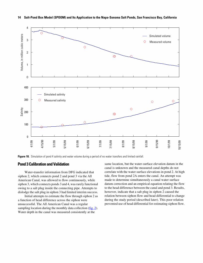
calculated from 1993 to 2001 data and used in the Evaporation worksheet. ............................................................ 13Figure 10. Graph showing simulation of pond 4 salinity and water volume during a period of

no water transfers and limited rainfall. ........................................................................................................................... 14Figure 11. Graph showing calibration, validation, and sensitivity analysis results for pond 3

from April 1, 1999, to October 1, 2001. .............................................................................................................................. 16Figure 12. Graph showing simulated nonzero flow rates determined through the calibration process for

pond 3 inflows and outflows. ............................................................................................................................................ 16Figure 13. Graph showing calibrated nonzero flow rates for pond 4 inflows and outflows. .................................................... 17Figure 14. Graph showing calibration, validation, and sensitivity analysis results for pond 4

from April 1, 1999, to July 1, 2001. ..................................................................................................................................... 17Figure 15. Graph showing calibration and validation results for pond 7 from April 1, 1999, to May 1, 2001. ......................... 19

Tables v

TABLESTable 1. Surface area and volume of ponds (assuming a water-surface elevation of

2 meters above sea level, NAVD 88). ............................................................................................................................... 4

vi Conversion Factors and Datum

Conversion Factors, Datum, Abbreviations, and Acronyms

CONVERSION FACTORS

Temperature in degrees Celsius (oC) may be converted to degrees Fahrenheit (oF) as follows:oF=1.8 oC+32.

VERTICAL DATUM

Vertical coordinate information is referenced to the North American Vertical Datum of 1988 (NAVD88).

ABBREVIATIONS and ACRONYMS

CIMIS California Irrigation Management Information System

DFG California Department of Fish and Game

USGS U.S. Geological Survey

A coefficient based on temperature, equation 2

Ad effective area for salt crystallization or dissolution, m2

B coefficient based on temperature, equation 3

Bv vapor transport coefficient, m/Pa*s

concentration of salt in solution, mol of salt/m3

saturated concentration of salt in solution at a given temperature, mol of salt/m3

C coefficient based on temperature, equation 4

Cp specific heat of air, J/kg*K

D diffusion coefficient of salt in water, m2/day

ea vapor pressure of air at z2, Pa

eas saturated vapor pressure of air at the surface, Pa

Multiply By To obtainmillimeter (mm) 0.03937 inch (in.)meter (m) 3.281 foot (ft)kilometer (km) 0.6214 mile (mi)hectare (ha) 2.471 acregram (g) 0.03527 ounce avoirdupois (oz)kilogram (kg) 2.205 pound avoirdupois (lb)square meter (m2) 10.76 square foot (ft2)cubic meter (m3) 35.31 cubic foot (m3)

c1

c1∗

Conversion Factors and Datum vii

EA evaporation from the Aerodynamic Method, mm/day

ER evaporation from the Energy Balance Method, mm/day

ET total evaporation rate, mm/day

k von Karman constant, 0.4

k1 average mass-transfer coefficient for salt dissolution, m/day

Kh heat diffusivity, m2/h

Kw vapor diffusivity, m2/h

lv latent heat of vaporization, J/kg

L characteristic length of the salt pond, m

molecular weight of salt, g/mol

P atmospheric pressure, kPa

R rate of salt crystallization or dissolution, kg of salt/day

Rn net radiation, W/m2

ReL Reynolds number,

S salinity

Sc Schmidt number,

T water temperature, �C

u velocity of the fluid above the salt bed, m/s

u2 wind speed measured at z2, m/s

z0 roughness height of the water surface, m

z2 height above water surface where u2 is measured, m

γ psychrometric constant, Pa/oC

∆ gradient of the saturated vapor pressure curve, Pa/oC

ρa density of air, kg/m3

ρo density of freshwater, kg/m3

ρw density of saltwater, kg/m3

µw viscosity of saltwater, kg/m*s

M2

ρw Ad 2⁄( )µw

-----------------------------

µw

ρwD-----------

Salt-Pond Box Model (SPOOM) and Its Application to the Napa-Sonoma Salt Ponds, San Francisco Bay, California

By Megan L. Lionberger, David H. Schoellhamer, Paul A. Buchanan, and Scott Meyer

ABSTRACT

A box model to simulate water volume and salinity of a salt pond has been developed by the U.S. Geological Survey to obtain water and salinity budgets. The model, SPOOM, uses the principle of conservation of mass to calculate daily pond volume and salinity and includes a salt crystallization and dissolution algorithm. Model inputs include precipitation, evaporation, infiltration, and water transfers. Salinity and water-surface-elevation data were collected monthly in the Napa-Sonoma Salt-Pond Complex from February 1999 through September 2001 and were used to calibrate and validate the model. The months when water transfers occurred were known but the magnitudes were unknown, so the magnitudes of water transfers were adjusted in the model to calibrate simulated pond volumes to measured pond volumes for three ponds. Modeled salinity was then compared with measured salinity, which remained a free parameter, in order to validate the model. Comparison showed good correlation between modeled and measured salinity. Deviations can be attributed to lack of water-transfer information. Water and salinity budgets obtained through modeling will be used to help interpret ecological data from the ponds. This model has been formulated to be applicable to the Napa-Sonoma salt ponds, but can be applied to other salt ponds.

INTRODUCTION

The Napa-Sonoma salt-pond system (figs. 1 and 2) is adjacent to northern San Pablo Bay and between Sonoma Creek and the Napa River. The ponds are contained by levees, which also serve as channel banks to a network of tidal sloughs (Warner and others, 2003). The pond land was originally tidal wetlands that were surrounded by levees in the 1850s and converted to farmland. In 1940, Leslie Salt Company, later acquired by the Cargill Corporation, bought

4,000 hectares (10,000 acres) of farmland. The land was flooded by water originating from San Pablo Bay, and salt was harvested and sold commercially until 1994, when the land was sold to the California Department of Fish and Game (DFG) to be maintained as ponds and restored as tidal wetlands (Nicholson and others, 2001). The ponds support large populations of migratory shorebirds and waterfowl (Takekawa and others, 2001).

Issues DFG has encountered during maintenance and restoration of the ponds are (1) how many and which ponds to restore to tidal wetlands, (2) how to manage pond salinities to provide ecological benefit, (3) how to dispose of excess salt, (4) how to restore selected ponds, and (5) what are the effects of proposed restoration alternatives on the local environment (Takekawa and others, 2000). From 1999 to 2001, the U.S. Geological Survey (USGS) collected ecologic and hydrologic data in the ponds to better understand how salinity and water depth affect pond biota. In order to interpret the ecological data, water and salinity budgets for the ponds must be determined. These budgets require quantification of precipitation, evaporation, water transfers between ponds, and salt crystallization and dissolution. Development of water and salinity budgets can be accomplished through modeling.

Purpose and Scope

This report documents a box model for salt ponds, SPOOM, and its application to the Napa-Sonoma salt-pond system. Specifically, this report describes model algorithms, model variables, test cases and sensitivity analysis, how to apply the model, the data used in this application, and calibration and validation of the model to the Napa-Sonoma salt-pond system. The model simulates the water volume and salinity of a salt pond using a mass-balance approach that considers rainfall, evaporation, salt crystallization and dissolution, infiltration, and water transfers.

2 Salt-Pond Box Model (SPOOM) and Its Application to the Napa-Sonoma Salt Ponds, San Francisco Bay, California

SAN PABLO BAY

SonomaCreek

122�30' 122�15' 122�00' 121�45'

38�15'

SanFranciscoEstuary

38�00'

37�45'

PACIFIC

OCEAN

CENTRAL BAY

SUISUN BAY

Sacramento/San JoaquinRiver Delta

Carquinez Strait

NapaRiver

PetalumaRiver

Golden Gate

Napa-SonomaSalt Ponds

0

0

0

0

5

5

10 Miles

10 kilometers

CALIF

O

R

N

IA

SAN PABLO BAY

SonomaCreek

122�30' 122�15' 122�00' 121�45'

38�15'

SanFranciscoEstuary

38�00'

37�45'

PACIFIC

OCEAN

CENTRAL BAY

SUISUN BAY


Carquinez Strait

NapaRiver

PetalumaRiver

Golden Gate


0

0

0

0

5

5

10 Miles

10 kilometers

CALIF

O

R

N

IA

SAN PABLO BAY

SonomaCreek

122�30' 122�15' 122�00' 121�45'

38�15'

SanFranciscoEstuary

38�00'

37�45'

PACIFIC

OCEAN

CENTRAL BAY

SUISUN BAY


Carquinez Strait

NapaRiver

PetalumaRiver

Golden Gate


0

0

0

0

5

5

10 Miles

10 kilometers

CALIF

O

R

N

IA

Figure 1. Napa-Sonoma salt-ponds study area, San Francisco Bay, California.

The purpose of the model application is to develop water and salinity budgets for the Napa-Sonoma salt-pond system. Salinity and water-surface-elevation data collected from February 1999 through September 2001 for the ponds were used to calibrate and validate the model. Bathymetric data were used to relate water-surface elevation and pond volume. The months when water transfers occurred were known but the magnitudes were unknown, so the magnitudes of water transfers were adjusted in the model to calibrate simulated pond volumes to measured pond volumes. Modeled salinity was then compared with measured salinity, which remained a free parameter, in order to validate the model. Simulated water and salinity budgets for ponds 3, 4, and 7 are included as worksheets in the SPOOM Excel file.

Acknowledgments

Thomas Huffman and Larry Wyckoff of DFG provided information regarding the operation of the Napa-Sonoma

ponds. Phillip Williams and Associates provided bathymetry data for the Napa-Sonoma ponds collected by the Towill Company and pan evaporation data collected by Cargill, Inc. Gregory Brewster, Paul Buchanan, Robert Sheipline, Brad Sullivan, and John Warner, USGS, collected the field data. William Bonnet and the Can Duck Club assisted with access to the sampling sites located in pond 2. Funding for this project was provided by the USGS Place-Based Program.

Description of the Study Area

The Napa-Sonoma salt ponds are separated from the adjacent tidal sloughs by levees. The levees were built by piling up soil removed from what is now the pond side of the levee. This created a borrow ditch along the inside of the ponds adjacent to the levee. The ponds conform to the shape of the tidal sloughs and were surveyed in 1999 (table 1). Canals, siphons, gates, and pumps were installed in the 1940s to control the flow of water between ponds.

Introduction 3

Sonoma

Creek

NapaRiver

San Pablo Bay

Intake Canal

CargillPump

38�08'

38�12'

122�25' 122�20'

0

0

3 Miles

5 kilometers

Pond 2

Pond 2A

Pond4

Pond3

Pond5

Pond1A

Pond1

Pond6A

Pond 6

Pond7A

Pond7

Pond8

AllAmerican

Canal

Pond9

Pond10

Crystallizers

Carneros#109

SouthSlough

ChinaSlough

Mud

Mud

EXPLANATIONSampling location

Siphon location

Sonoma

Creek

NapaRiver

San Pablo Bay

Intake Canal

CargillPump

38�08'

38�12'

122�25' 122�20'

0

0

3 Miles

5 kilometers

Pond 2

Pond 2A

Pond4

Pond3

Pond5

Pond1A

Pond1

Pond6A

Pond 6

Pond7A

Pond7

Pond8

AllAmerican

Canal

Pond9

Pond10

Crystallizers

Carneros#109

SouthSlough

ChinaSlough

Mud

Mud

EXPLANATIONSampling location

Siphon location

Figure 2. Napa-Sonoma salt-pond complex, California. Carneros #109 indicates the location of the California Irrigation Management Information System (CIMIS) meteorological station. See figure 1 for location of ponds.


Table 1. Surface area and volume of ponds (assuming a water-surface elevation of 2 meters above sea level, NAVD 88)

[See fig. 2 for location of ponds]

Pond number

Surface area (square meters)

Volume (cubic meters)

1 1,500,000 1,558,000

1A 2,321,000 2,166,000

2 3,070,000 4,058,000

2A 2,086,000 2,810,000

3 5,216,000 4,679,000

4 3,786,000 4,682,000

5 3,145,000 4,007,000

6 2,968,000 3,201,000

6A 1,772,000 1,929,000

7 1,239,000 1,554,000

7A 1,238,000 1,531,000

8 454,000 1,094,000

Salt was produced by evaporation of water from the ponds, leaving the salt for harvesting. A dry season extends from spring through fall, during which time evaporation exceeds rainfall. Water from San Pablo Bay was allowed to flow into pond 1 at high tide when a gate was open. Water from pond 1 was pumped into pond 2 and flowed by gravity sequentially through the ponds. The ponds were a closed system, and therefore salinity increased from one pond to the next. The water was transferred from pond 8 to the east side of the Napa River, where the evaporation process was completed and the salt harvested.

A levee breach opened pond 2A to tidal action in 1995. Since then, pond 2A has become a vegetated marsh plain. Pond 2, where the Can Duck Club is located, is connected to pond 3 by the All American Canal. During high tides, water flows into the All American Canal from pond 2A through a drain flap gate. Ponds 4 and 5 are connected by a 3.7-m-wide levee breach opened in 1996.

During this study, water was supplied to the pond system by tidal exchange in ponds 1 and 2 in the south, by Napa River water pumped into the system from the north, and by rainfall. Tides affected pond 1 by way of an intake canal connecting the pond to San Pablo Bay (fig. 2). This is the main inlet for flow into the salt-pond system. Pond 2 also can

be tidally influenced by two weirs with flap valves, one on the east side of the pond and one on the west side, that allow water to enter the pond from China Slough and South Slough, respectively (fig. 2). Ponds 3 through 8 are not directly influenced by tidal action.

Altered pond management and deteriorating infrastructure prevented development of hydraulic heads capable of moving pond water by gravity sequentially from one pond to the next through the entire series of ponds as originally designed. Alternatively, Cargill, Inc. pumped Napa River water into a canal network connecting the northernmost ponds to the eastern side of the Napa River (ponds 9, 10, and Crystallizers; see fig. 2). The amount of time the pump was run was limited by DFG funds, which bore the cost of the electricity to operate the pump (72 days in 1999; 107 days in 2000).

During the study, semi-permanent salt plugs formed between siphons connecting ponds 3 and 4, and ponds 5 and 6 (fig. 2). Salt plugs consist of relatively dense water that the head difference across a siphon is unable to move, preventing the flow of water. Attempts to dislodge the salt plugs by DFG were rarely successful. As a result, ponds 4 and 5 went dry over the summer of 2001.

Model Description 5

The Napa-Sonoma salt ponds are located within the Pacific Flyway and serve as staging and wintering areas for migratory waterfowl and shorebirds. More than 90 percent of historical wetlands of San Francisco Bay have been lost to human development, and waterfowl and shorebirds are found in higher densities on salt ponds than bayland wetlands. Proposed restoration of the salt ponds to tidal marsh will reduce waterbird habitat in San Francisco Bay and will increase wetlands habitat (Takekawa and others, 2001).

DATA COLLECTION

Specific conductance, water temperature, salinity, pH, dissolved oxygen, turbidity, and water-surface elevation were measured at discrete locations within the ponds (fig. 2). A Hydrolab Minisonde was used to make all measurements except those for water-surface elevations; these were taken from staff plates in each pond. Water-surface elevation measurements are sometimes missing because the staff plates could be on dry land when the water level was low. The Hydrolab Minisonde was calibrated in the field to known standards and the calibration was checked intermittently to assure sensor performance. Measurements were taken once a month from ponds 1, 2, 2A, 3, 4, and 7 between February 1999 and September 2001; measurements continued to be taken bimonthly at ponds 3 and 4 through 2002. In ponds 1, 3, 4, and 7, the instrument was placed in the shade created by the hydrographer (direct sunlight can affect certain parameters such as turbidity). After the instrument equilibrated and any disturbed sediment settled, measurements were taken and recorded on a field sheet. Pond 2 measurements were taken both from a dock and a boat, and pond 2A measurements were taken from a walkway. Measurements were taken at one point in the water column except when the depth exceeded 1 m; then two measurements were taken to help define any vertical stratification.

Ionic composition of salts in solution was assumed to be similar to seawater and dominated by sodium chloride. Data for sodium chloride brine were used to estimate the hyper-saturated water properties in the ponds because of a lack of hyper-saturated-seawater data (see Appendix). The validity of this assumption decreases in the latter ponds owing to salt crystallization and dissolution. The salts still remaining in

solution by the time water gets to pond 7 are more likely to have higher saturation concentrations.

Salinity is computed by the Hydrolab Minisonde using the 1978 Practical Salinity Scale (Fofonoff and Millard, 1983). This algorithm is defined for salinities ranging from 2 to 42 (dimensionless), although it is used by the instrument to calculate salinities up to 70. As a reference for comparison of scale, seawater has a salinity of 35 and freshwater has a salinity of 0. ERTCO, a hydrometer manufacturer, provided a conversion table of specific gravity and temperature to salinity for sodium chloride brine up to the saturation salinity 264 (specific gravity of 1.204). Comparison of simultaneous salinity measurements from the Minisonde and a hydrometer ranging between 42 and 70 shows a lack of agreement (fig. 3). Salinities from 42 to 70 measured using the Minisonde were corrected to be consistent with hydrometer measurements. Hydrometers were used exclusively to obtain specific gravity data when salinities in the ponds exceeded 70. The conversion between specific gravity and salinity provided by ERTCO for salinities that are under-saturated is linear. These data were extrapolated to calculate salinities for hyper-saturated conditions after no other conversion scale was found.

Figure 4 shows the data series measurements of salinity for ponds 1, 2, 2A, 3, 4, and 7. In all ponds, salinity increases in the summer during the dry season and decreases in the winter during the rainy season. Overall, salinities tend to increase over time.

MODEL DESCRIPTION

The salt-pond box model (SPOOM) represents a single salt pond, in a salt-pond evaporation system, as a well-mixed box of saltwater. SPOOM balances both water volume and salt mass using the principle of conservation of mass. Water transfers, rainfall, and evaporation are accounted for by the mass balance calculations (fig. 5). An infiltration rate can also be included. The model calculates volume (in cubic meters) and salinity (1978 Practical Salinity Scale, dimensionless) for a specific pond and range of time specified by the user, with a daily time step. The user can also define the pond geometry and modify rainfall and evaporation rates, thus making the model generally applicable to other salt ponds.


0 10 20 30 40 50 60 70 80 900

30

60

90

Hydrolab minisonde salinity

Hydr

omet

ersa

linity

Figure 3. Salinity as measured by the Hydrolab Minisonde salinity and the hydrometer salinity. Note that the line with a one-to-one slope represents agreement between the Hydrolab Minisonde and the hydrometer measurements.

2/1/99 6/1/99 10/1/99 2/1/00 6/1/00 10/1/00 2/1/01 6/1/01 10/1/0110 0

10 1

10 2

10 3

Salin

ity

Pond 1Pond 2Pond 2APond 3Pond 4Pond 7

EXPLANATION

Figure 4. Salinity measurements for ponds 1, 2, 2A, 3, 4, and 7 from February 1999 through September 2001. See figure 2 for location of ponds.

Model Description 7

SPOOM VariablesEvaporation

Infiltration

Rainfall

Inflow Outflow

Pond

Figure 5. Salt-pond box-model variables. The uncolored arrow indicates an optional variable.

SPOOM was written as a program in Visual Basic for Excel and is located within the Excel file SPOOM.xls. The worksheets found inside the Excel workbook include the Main worksheet, the Rainfall worksheet, the Evaporation worksheet, the InflowOutflow worksheet, and the Results worksheet. The Main worksheet consists of the user input page and graphical results page. The user enters the start date, end date, pond number, and type of rain year into the corresponding spreadsheet cells. Daily water-volume loss owing to infiltration can be entered in cell H2, although this is optional. The Rainfall and Evaporation worksheets list daily rainfall and evaporation values, in millimeters. The InflowOutflow worksheet lists the daily inflow and outflow, in cubic meters, and the corresponding inflow salinity. Outflow salinity is calculated by SPOOM. The Results worksheet serves as the output table for the model. Daily

values of water volume, salinity, salt mass, pond area, pond depth, rainfall, and evaporation are listed. Each time the model is initiated, the results table is cleared; at the end of the model run, dates and output values are automatically updated.

SPOOM is activated by pressing the control key and the m key simultaneously. The model steps through the calculations by daily intervals. For each time step, SPOOM collects data for daily rainfall, evaporation, water transfers, and, if entered, the infiltration rate. The model uses these values to calculate the loss or gain in salt mass and water volume in the pond. Once the calculations are complete, the graphs of salinity, pond volume, and rainfall/evaporation summary are updated using the daily values listed on the Results worksheet. Figure 6 details the algorithm used by SPOOM to make these calculations.

New Pond Model (Sal-lookup)\generic new pond model-Sal Lookup.xls


Select start and end datesSelect pond numberSelect rainfall type

Select infiltration rate (optional)

Calculate change in water volumeand salt mass from inflow

Add or remove salt mass in concentrationfrom salt crystallization or dissolution

Calculate change in water volume from infiltration

Calculate change in water volume from precipitation

Calculate change in water volume from evaporation

Calculate change in water volumeand salt mass from outflow

Get variables for current dayfrom worksheets

(Rainfall, Evaporation, InflowOutflow)

Write data to Resultsworksheet

NoYesUpdate graphs on

the Main worksheetGo to next day

Are theremore days to

calculate?

Figure 6. Salt-pond box-model (SPOOM) algorithm.

Model Description 9

Rainfall

Daily rainfall is multiplied by the drainage area of the pond, usually slightly greater than the wetted surface area, to determine the volume of water added to the pond from precipitation. The salinity of rainfall is assumed to be zero.

Evaporation

The user provides a daily time-series of freshwater evaporation rates in the Evaporation worksheet. Salinity increases water density, consequently reducing evaporation to less than the freshwater value. To account for this, the model applies a correction factor to reduce evaporation. An equation relating water density to salinity (S) is given by Millero and Poisson (1981):

(1)

where ρw is the salt water density and ρo is the reference freshwater density. The variables A, B, and C are coefficients based on temperature (T, Celsius):

(2)

(3)

(4)

The density of freshwater is also a function of temperature and is calculated as:

(5)

An algorithm adjusts the value for water density and the daily freshwater evaporation rates listed in the Evaporation worksheet using the previous day’s salinity, equation 1, and an assumed temperature of 19.3oC, corresponding to the average temperature measured in ponds 3, 4, and 7 during this study. The adjusted evaporation rate is multiplied by the surface area of the pond to determine the water volume removed. The salt mass in the pond is assumed to be unaffected by evaporation.

The freshwater evaporation rates listed in the Evaporation worksheet are specifically calculated for the

northern San Pablo Bay region. Because evaporation rates vary from location to location, these rates may need to be recalculated for another location. The new rates can be pasted over the existing evaporation rates in the Evaporation worksheet. The density correction algorithm will continue to adjust the evaporation rates to reflect salinity without any further modification by the user.

Salt Crystallization and Dissolution

Salt in solution becomes hyper-saturated when salinity exceeds 264. Under hyper-saturation conditions, salt crystallizes and drops out of suspension. The salt crystals adhere to the bottom of the pond forming a salt crust. This process effectively reduces the salinity in the water column until it reaches an equilibrium saturation condition (264). Under hypo-saturation conditions where salinity is less than 264 and crystallized salt is present, salt is dissolved back into suspension raising salinity until all the crystallized salt is dissolved or equilibrium saturation is reached.

The rate of salt crystallization or dissolution (R), as described by Manganaro and Schwartz (1985), is

(6)

where

The average mass-transfer coefficient for salt dissolution (k1) is given by

(7)

where

The characteristic length used in the calculation of both ReL and k1 is taken as the square root of the area of the pond. The velocity of the fluid above the bed is assumed to be 25 mm/s in the calculation of ReL (Jeremy Bricker, Stanford University, written commun., 2001) and D is assumed to be 2.0 × 10-9m2/s. No data were available to validate or calibrate this submodel.

ρw ρo AS BS32---

CS2+ + +=

A 8.24493 1–× 10 4.0899 3–× 10 T 7.6438 5–× 10 T+–2

=

8.2467 7–× 10– T3 5.387 9–× 10+ T4

B 5.72466x– 10 3– 1.0227x10 4–+ T 1.6546x10 6–– T2=

C 4.8314 4–× 10=

ρo 999.842594 6.793952 2–× 10 T 9.095290 3–× 10–+( )T2=

1.001685 4–× 10 T3 1.120083–6–× 10+ T4 6.536332+

9–× 10 T5+

is the average mass-transfer coefficient for salt dissolution

Ad is the wetted areais the concentration of salt in solutionis the saturated concentration of salt in

solution at a given temperatureis the molecular weight of salt

ReL is the Reynolds numberSc is the Schmidt numberD is the diffusion coefficientL is the characteristic length of the salt pond

R k1Ad c1 c1∗

–( )M2=

k1

c1

c1∗

M2

k10.664ReL

12---

Sc13---

DL

---------------------------------------=


An algorithm in the model checks if salt in solution is hyper-saturated or if it is hypo-saturated with a crystallized salt mass. If either condition exists, equation 6 will adjust the salt mass in solution.

Water Transfers

The model requires that pond inflow, but not outflows, be assigned a salinity value. SPOOM continuously calculates pond salinity and applies this number to outflows to determine the mass of salt removed from a pond. If there is neither an inflow nor an outflow on a given date, all cells except that for the date are left blank in that row in the InflowOutflow worksheet. An initial water volume and salinity must be entered on the date that corresponds with the start date chosen by the user on the Main worksheet.

Pond Geometry

The change in pond volume from rainfall is calculated by multiplying the daily rainfall depth by the maximum basin area for each pond to incorporate surface runoff from the levees. Similarly, the water-surface area at a given water-surface elevation is used to determine the volume change due to evaporation. If a water-surface elevation happens to fall between entries listed in the Geometry worksheet, a subroutine uses interpolation to determine the pond area and volume.

Analytic Test Cases

Three tests with analytic solutions demonstrated that the model calculations were correct and that the model conserved water volume and salt mass, using the following three test cases: 1) no inflow, no outflow, constant rainfall rate, and no evaporation, 2) no inflow, constant outflow, no rainfall, and no evaporation, and 3) an initial nonzero pond salinity with inflow equal to outflow, and inflow salinity equal to zero. The results of these tests agreed with the analytic solutions and showed the pond to overflow in case 1 and go dry in case 2, and the salinity to go to zero in case 3.

APPLICATION OF THE MODEL TO THE NAPA-SONOMA SALT PONDS

SPOOM, outlined above, was applied to the Napa-Sonoma salt ponds. Data sets and algorithms were developed for rainfall, evaporation, infiltration, water transfers, and pond geometry.

Rainfall

Rainfall data collected by the California Irrigation Management Information System (CIMIS) were used to determine the volume of water added to the ponds by precipitation. CIMIS weather station, Carneros #109 (fig. 2), is within 16 km of all pond sampling locations and has been collecting meteorological data since March 1993. The daily rainfall values recorded at Carneros were assumed to represent the rainfall on the ponds.

For future scenario development and hypothetical modeling, SPOOM includes three rainfall scenarios representing an average (normal) year, a dry year, and a wet year. A representative average rainfall year (567.7 mm) was created by calculating the mean rainfall for every day of the year for the entire period of record (March 1993–July 2001). The dry year and wet year rainfalls were the driest and wettest complete yearly rainfall records recorded at Carneros (1994–2001). They are years 1999 (196.5 mm) and 1995 (882.5 mm) (fig. 7).

Evaporation

Theoretical daily freshwater evaporation rates calculated by the Combined Aerodynamic and Energy Balance Method (Chow and others, 1998) were summed to derive monthly evaporation rates, which were compared to average monthly Weather Bureau Class A pan evaporation data (1993–2001) recorded by Cargill at a site within the Napa-Sonoma salt-pond complex. The comparison showed that monthly evaporation rates for the Combined Aerodynamic and Energy Balance Method were between 0.69 and 0.82 of the pan evaporation rates (fig. 8), which falls within or near an acceptable range of 0.67 to 0.81 given by the World Meteorological Organization (World Meteorological Organization, 1966). Thus, this method was chosen to simulate evaporation for the Napa-Sonoma salt ponds.

The Combined Aerodynamic and Energy Balance Method (Chapra, 1997) gives the total evaporation rate, ET:

(8)

whereis the gradient of the saturated vapor pressure

curveγ is a psychrometric constant

ER is evaporation from the Energy Balance MethodEA is evaporation from the Aerodynamic Method

ET∆

∆ γ+-------------ER

γ∆ γ+-------------EA+=

∆



Application of the Model to the Napa-Sonoma Salt Ponds 11

Jan. 1 Mar. 1 May 1 July 1 Sept. 1 Nov. 1 Jan. 10

20

40

60

80

100

120

NORMAL(1993-2001MEAN DAILY)

DRY (1999)

WET (1995)

RAINFALL YEAR:

Daily

rain

fall,

inm

illim

eter

s

Figure 7. Daily rainfall rates, in millimeters per day, for normal, dry, and wet years, used in the Rainfall worksheet.

The weighting factors ∆/(∆+γ ) and γ /(∆+γ ) sum to unity and are defined as

(9)

and

(10)

where

The evaporation due to incoming net radiation, ER, is given by

(11)

where

The evaporation due to vapor transport, EA, is given by

(12)

where ea is vapor pressure, and the vapor transport coefficient, Bv, is

(13)

where

The meteorological data required for these calculations are air temperature, net radiation (Rn), relative humidity, and wind speed (u2); these were obtained from the CIMIS Carneros weather station. In addition to the daily values, a representative set of daily freshwater evaporation rates for use in hypothetical scenarios was compiled from the daily averages of the calculated evaporation rates (fig. 9) using data collected at the weather station from March 1993 to December 2001. These are the evaporation rates given in the Evaporation worksheet. For model calculations, the pond temperature is assumed to be 19.3�C, corresponding to the average temperature measured in ponds 3, 4, and 7 during this study.

eas is the saturated vapor pressure of air

T is water temperatureCp is the specific heat of airKh is heat diffusivityP is atmospheric pressurelv is the latent heat of vaporization

Kw is vapor diffusivity

Rn is net radiationρo is the density of freshwater

∆4098eas

237.3 T+( )2------------------------------=

γCpKhP

0.622lvKw-------------------------=

ERRn

lvρo----------=

EA Bv eas ea–( )=

k is the von Karman constantρa is the density of airu2 is wind speedz2 is the height above the water where u2 is

measuredz0 is the roughness height of the water surface

Bv0.622k2ρau2

Pρo z2 z0⁄( )ln[ ]2--------------------------------------------=


Janu

ary

Febr

uary

Mar

ch

April

May

June

July

Augu

st

Sept

embe

r

Octo

ber

Nov

embe

r

Dece

mbe

r

0

50

100

150

200

250

EXPLANATION

Aver

age

cum

ulat

ive

mon

thly

evap

orat

ion,

inm

illim

eter

s

Combined aerodynamic and energy balance method evaporationCargill pan evaporation

Figure 8. Average cumulative monthly evaporation for the Combined Aerodynamic and Energy Balance Method and Cargill pan data (1993–2001).

The Combined Aerodynamic and Energy Balance Method was tested on pond 4 during a period with very little rainfall and no water transfers, so only evaporation significantly altered water level and salinity. A simulation was run using pond 4 data collected from April to October 1999, during which time evaporation is at its highest for the year, to compare simulated volumes to measured volumes. Results of this simulation (fig. 10) show good correlation between modeled and measured volume and the salinity.

Infiltration

Infiltration rates are assumed negligible. Studies have shown that infiltration rates can be quite large for newly constructed ponds, but then decrease to very small amounts after a few months owing to plugging of conducting pores in the bed material by microbial slimes and colloidal soil materials (Madramootoo and others, 1997). Considering the age of the ponds, applying a zero infiltration rate is an acceptable assumption.

Water Transfers

DFG regulates the transfer of water between the Napa-Sonoma salt ponds. A list of the months in which water was transferred between ponds was obtained from DFG and used as a constraint on the model runs. The constrained water-transfer rates were adjusted to calibrate simulated pond-water volumes to measured pond-water volumes. Salinity measurements from the All American Canal and pond 3 were used as inflow salinities to ponds 3 and 4, respectively. Daily salinity values were interpolated between monthly salinity measurements. Inflow salinity to pond 7 was not measured. A salinity of 15 was assumed for all inflows into pond 7 resulting from pumping of Napa River water by Cargill.

Pond Geometry

The Geometry worksheet summarizes the volumes and surface areas based on pond water-surface elevations according to the vertical datum NAVD 88. The geometry data were compiled using Napa-Sonoma salt-pond-complex survey data collected by the Towill Company.

Model Calibration and Validation 13

Jan.

1

Feb.

1

Mar

.1

Apr.

1

May

1

June

1

July

1

Aug.

1

Sept

.1

Oct.

1

Nov

.1

Dec.

1

Jan.

1

0

2

4

6

8

Daily

evap

orat

ion,

inm

illim

eter

spe

rday

Figure 9. Representative daily evaporation rates, in millimeters per day, calculated from 1993 to 2001 data and used in the Evaporation worksheet.

MODEL CALIBRATION AND VALIDATION

The factors that alter the water volume and salinity of the ponds are rainfall, evaporation, salt crystallization and dissolution, and water transfers. Rainfall is well known from measured data, and evaporation is satisfactorily determined from meteorological data and the Combined Aerodynamic and Energy Balance Method (fig. 10). Salt crystallization is important only under hyper-saturated conditions and salt dissolution only after hypo-saturated conditions are restored; the rate of crystallization or dissolution is calculated using equation 6. Some water transfers are known from DFG records of flow occurrence, but the magnitude of the water transfers is unknown.

In order to close the water and salinity budgets, the model was used to determine the magnitude of the water transfers so that the simulated pond volumes closely matched the measured pond volumes. In other words, the calibration parameter of the model was the magnitude of water transfers between ponds. A constant flow rate was determined for each period between monthly measurements. The simulated water transfers were constrained by the physical dimensions and conditions of the water-transfer infrastructure (pond connections), the months when DFG recorded flow, and conservation of mass such that the outflow from one pond

was the inflow to another. Special cases of water transfers determined from field observations and information from DFG were leaky gates and blocked siphons. These special situations were included in the modeling of the affected ponds.

Whereas the constrained water transfers were adjusted so that the simulated pond volumes matched the observed pond volumes, salinity was not used in the calibration process and thus provides a form of model validation. Because of this approach, simulated salinities are not expected to match the data as well as simulated water volumes. Agreement between simulated and measured salinities would indicate that the model assumptions, simulated processes, and utilization of field data are a good representation of reality, whereas discrepancies would indicate that they are imperfect.

The model was calibrated for only the nontidal ponds where data had been collected. Initial simulation runs showed that SPOOM was unable to model the tidally influenced ponds. The variability of flows during a tidal cycle could not be accurately described with an average flow rate for a daily time step. Therefore, calibration was done for ponds 3, 4, and 7 only. The outflows applied to pond 3 were inserted into pond 4 as inflows. Final calibrations of both ponds were performed simultaneously. Details of all three calibrations are discussed below.



0

1

2

3

4

0

100

200

300

400

4/1/

99

4/15

/99

5/1/

99

5/15

/99

6/1/

99

6/15

/99

7/1/

99

7/15

/99

8/1/

99

8/15

/99

9/1/

99

9/15

/99

10/1

/99

10/1

5/99

Simulated volume

Measured volume

Simulated salinity

Measured salinity

Volu

me,

inm

illio

ncu

bic

met

ers

Salin

ity

0

1

2

3

4

0

100

200

300

400

4/1/

99

4/15

/99

5/1/

99

5/15

/99

6/1/

99

6/15

/99

7/1/

99

7/15

/99

8/1/

99

8/15

/99

9/1/

99

9/15

/99

10/1

/99

10/1

5/99

Simulated volume

Measured volume

Simulated salinity

Measured salinity

Volu

me,

inm

illio

ncu

bic

met

ers

Salin

ity

0

1

2

3

4

0

100

200

300

400

4/1/

99

4/15

/99

5/1/

99

5/15

/99

6/1/

99

6/15

/99

7/1/

99

7/15

/99

8/1/

99

8/15

/99

9/1/

99

9/15

/99

10/1

/99

10/1

5/99

Simulated volume

Measured volume

Simulated salinity

Measured salinity

Volu

me,

inm

illio

ncu

bic

met

ers

Salin

ity

Figure 10. Simulation of pond 4 salinity and water volume during a period of no water transfers and limited rainfall.

Pond 3 Calibration and Validation

Water-transfer information from DFG indicated that siphon 2, which connects pond 2 and pond 3 via the All American Canal, was allowed to flow continuously, while siphon 3, which connects ponds 3 and 4, was rarely functional owing to a salt plug inside the connecting pipe. Attempts to dislodge the salt plug in siphon 3 had limited interim success.

Initial attempts to estimate the flow through siphon 2 as a function of head difference across the siphon were unsuccessful. The All American Canal was a regular sampling location during the monthly data collection (fig. 2). Water depth in the canal was measured consistently at the

same location, but the water-surface elevation datum in the canal is unknown and the measured canal depths do not correlate with the water-surface elevations in pond 2. At high tide, flow from pond 2A enters the canal. An attempt was made to determine simultaneously a canal water-surface datum correction and an empirical equation relating the flow to the head difference between the canal and pond 3. Results, however, indicate that a salt plug in siphon 2 caused the relation between siphon flow and head differential to change during the study period (described later). This poor relation prevented use of head differential for estimating siphon flow.


Better results were obtained when modeled volumes were fit to measured volumes using mass balance to simplify the calculation of the flow rate through siphon 2. This approach provides less constraint on the flow through siphon 2. Periods of outflow indicated by the mass-balance calculations and DFG data were also applied to pond 4. Adjustments were made to the inflows and outflows of pond 3 while preserving the mass balance until the modeled pond 4 water volumes closely matched the measured volumes. The modeled daily salinity values of both ponds were compared to measured values to validate model performance.

Analysis of the data collected in the All American Canal and pond 3 between November 1999 and April 2000 indicates that there was little or no flow through siphon 2. DFG water- transfer data indicate that there was no flow leaving the pond through siphon 3 during this period. It is hypothesized that a period of slack flow in siphon 2 allowed a salt plug to form within the siphon. Depths recorded in the canal during March and April were greater than at all other times during the data-collection period. During May 2000, a large volume of water moved from pond 3 to pond 4 when a salt plug in siphon 3 was dislodged. The water-surface elevation in pond 3 dropped 0.4 m. This increased the head differential between the All American Canal and pond 3, which dislodged the salt plug in siphon 2. Thereafter, free flow of water through siphon 2 resumed. The salt plug in siphon 2 was simulated by assuming no inflow to pond 3 from November 12, 1999, to May 28, 2000. Figure 11 shows the pond 3 calibration and validation results. The effect of the decreased outflow will be explained in the forthcoming sensitivity analysis section for ponds 3 and 4.

The pond 3 salinity results are in excellent agreement with the measured salinity until an unusual simulated increase between July and November 2000. A separate model run (not shown) was made that adjusted the flow into and out of pond 3 to fit the measured salinity values, but the results had pond 4 overtopping its levees and an underestimate of the salinity in pond 3 during the remaining period of the run. It is unclear why this salinity increase does not occur in the measured data, because the measured volume decreases during the months of June through August. DFG records and results of pond 4 modeling indicate that there was no flow through siphon 3 (out of pond 3) until November 2000. The law of conservation of mass states that when there is a net decrease in volume and no outflow, salinity must increase, as the model results show. Thus, this discrepancy between the simulated and measured salinities is unexplained. After November 2000 the simulated salinities covary with the measured values but are slightly greater. Figure 12 shows both the simulated inflow and outflow rates determined through the calibration process for pond 3. The simulated water and salinity budgets for pond 3 are included as a worksheet in the SPOOM excel file.


Pond 4 is connected to pond 5 by a 3.7-m-wide breach in the levee separating the two ponds. SPOOM assumes ponds 4 and 5 to be two separate ponds because the breach is small relative to the overall size of the ponds, thus preventing the ponds from becoming instantaneously well mixed (a fundamental assumption of the model). An initial calibration effort using the assumption that the two ponds acted as one well-mixed pond gave poor results. Because no data were collected in pond 5, modeled values could only be compared with pond 4 data. Model calibration indicated that flow through the breach between ponds 4 and 5 was negligible except in May 2000.

Flow enters pond 4 through siphon 3, which connects pond 3 to pond 4. Flow rates through this siphon were determined by parallel calibration of ponds 3 and 4, as described above. Most of the flows through siphon 3 are generally small when they do occur, because of the salt plug (fig. 13). When flows were small or zero, zero outflow through the levee breach to pond 5 was assumed. This was not the case for the large outflow from pond 3 in May 2000. Using mass balance in pond 3 to calculate flow through siphon 3 overpredicted the volume in pond 4 if no outflow was assumed. In this case, water obviously was leaking through the levee breach. Model calibration showed that when 35,000 m3/day entered pond 4, 10,000 m3/day was flowing into pond 5.

Figure 14 shows the calibration results of pond 4. The simulated water and salinity budgets for pond 4 are included as a worksheet in the SPOOM Excel file. Modeled salinities were consistently higher in late fall 1999 and 2000 after the peak summer evaporation periods. Otherwise, modeled salinity showed reasonable correlation to measured salinity. The model only ran to July 2001 because the pond dried shortly afterward and stayed dry until winter, making data collection impossible. The effect of the decreased outflow will be explained in the forthcoming sensitivity analysis section for ponds 3 and 4.

Sensitivity Analysis of Water Transfers for Ponds 3 and 4

Model results are sensitive to the value of the calibration parameter of water-transfer rate. To demonstrate this, the calibrated flow rates between ponds 3 and 4 were decreased by 20 percent. Model results are shown as green lines in figures 11 and 14. Even though there is no flow between ponds most of the time, results for both ponds are worse with this smaller flow rate. The salinity match improves for pond 3, but the volume is overpredicted. For pond 4, pond volume is underpredicted and salinities are overpredicted.


0

1

2

3

4

5

6

0

20

40

60

80

100

120

4/1/

99

6/1/

99

8/1/

99

10/1

/99

12/1

/99

2/1/

00

4/1/

00

6/1/

00

8/1/

00

10/1

/00

12/1

/00

2/1/

01

4/1/

01

6/1/

01

8/1/

01

10/1

/01

MINIMUM MEASURABLE WATER LEVEL

Simulated salinityMeasured salinityDecreased outflow (sensitivity analysis)

Simulated volumeMeasured volumeDecreased outflow (sensitivity analysis)

Volu

me,

inm

illio

ncu

bic

met

ers

Salin

ity

Figure 11. Calibration, validation, and sensitivity analysis results for pond 3 from April 1, 1999, to October 1, 2001.

4/1/

99

6/1/

99

8/1/

99

10/1

/99

12/1

/99

2/1/

00

4/1/

00

6/1/

00

8/1/

00

10/1

/00

12/1

/00

2/1/

01

4/1/

01

6/1/

01

8/1/

01

10/1

/01

0

10

20

30

40

50

Inflow

outflow

Daily

flow

rate

,in

thou

sand

cubi

cm

eter

s

Figure 12. Simulated nonzero flow rates determined through the calibration process for pond 3 inflows and outflows.


4/1/

99

6/1/

99

8/1/

99

10/1

/99

12/1

/99

2/1/

00

4/1/

00

6/1/

00

8/1/

00

10/1

/00

12/1

/00

2/1/

01

4/1/

01

6/1/

01

0

10

20

30

40

Inflow

Outflow

Daily

flow

rate

,in

thou

sand

cubi

cm

eter

s

Figure 13. Calibrated nonzero flow rates for pond 4 inflows and outflows.

0

1

2

3

4

0

100

200

300

400


SALT SATURATION POINT

4/1/

99

7/1/

99

10/1

/99

1/1/

00

4/1/

00

7/1/

00

10/1

/00

1/1/

01

4/1/

01

7/1/

01

Simulated volumeMeasured volumeDecreased outflow (sensitivity analysis)

Volu

me,

inm

illio

ncu

bic

met

ers

Salin

ity

Simulated salinityMeasured salinityDecreased outflow (sensitivity analysis)

Figure 14. Calibration, validation, and sensitivity analysis results for pond 4 from April 1, 1999, to July 1, 2001.



Pond 7 had a salt crust during the entire study. The only gate structure connecting pond 7 to the pond system was continuously closed during the data-collection period, but allowed a small amount of flow into the pond during periods when water was pumped into the system from the north by Cargill. The dates when pumping occurred were obtained from DFG (May 18–June 30, 1999; September 30–October 29, 1999; February 25–May 6, 2000; and May 25, 2000–June 30, 2000), and a constant inflow rate of 3,500 m3/day was applied to those dates. This value was determined by calibrating simulated pond volume to measured pond volume. DFG repaired the gate on August 17, 2000. The inflow rate was assumed to be zero after the leak was fixed.

Figure 15 shows the pond 7 calibration and validation results. The results showed good correlation with measured salinity values for the hyper-saturated pond. The model did not overestimate the salinity after the pond became hyper-saturated, indicating that the salt crystallization algorithm was taking salt out of solution at an appropriate rate. The simulated water and salinity budgets for pond 7 are included as a worksheet in the SPOOM Excel file.

Discussion

Modeled pond volumes were fit to the measured pond volumes by adjusting water transfers in and out of each pond. Water transfers were constrained by conservation of mass between ponds and by the dates when DFG intentionally transferred water. In addition, salt plugs blocking siphons and leaky gates were considered.

Salinity was reserved as a free parameter to validate model results against measured data. In general, the simulated salinities and the temporal variability of salinity were in good agreement with data, but sometimes the model overestimated salinity. There are several possible explanations. Periods of flow between ponds are imprecisely known. The siphon inlets and outlets are located below the water surface so it is often difficult, if not impossible, to tell that a siphon is actually flowing. Not all leaks and salt plugs during the study period may be known. The mean of salinity measured typically at four points in a pond is assumed to be equal to the mean pond salinity, but may not always represent well the salinity in a pond. The assumption that a pond is well mixed may not always be valid. Meteorological data from Carneros was assumed to be applicable to the ponds, but the Carneros station is inland from the ponds and probably is sometimes sunnier and warmer, which could result in an overestimation of evaporation parameters. The results presented in figures 11, 14, and 15 represent the best, but

sometimes imperfect, estimates of the water and salinity budgets for ponds 3, 4, and 7.

Seasonal variability results in large fluctuations in pond salinity and volume due to evaporation. Salinity shifts of 60 in pond 3 and 200 in ponds 4 and 7 are common between winter and summer. Pond 4 becomes hyper-saturated during late summer, forming a salt crust which then dissolves during the winter when evaporation rates are reduced and rainfall lowers the salinity in the pond. Over the 2-year study period there is a trend of increasing salinity in all three ponds. Ponds 3 and 4 are supplied more by saline water from the bay than freshwater from rainfall, resulting in a buildup of salt mass and increased salinity. Pond 7 does not receive enough rainfall and unintended inflow to replace evaporated water.

OTHER MODEL APPLICATIONS

The generic pond model can be used to make predictions for a prescribed scenario for the Napa-Sonoma salt ponds. An initial volume and salinity must be listed on the InflowOutflow worksheet as an inflow on the first date the model is scheduled to run. In addition, the user must choose the type of rainfall year, and the inflow and outflow rates. A string of ponds can be connected in series and the flows coordinated between them. It must be kept in mind that water transfers between most ponds are due to gravity and require a head differential between the ponds. There is no safety feature in SPOOM that checks that the water-surface elevation of the discharging pond exceeds that of the receiving pond.

The generic model is not confined to run only for a single year. The data in the Rainfall, Evaporation, and InflowOutflow worksheets can be extended to cover a longer period. The rainfall and evaporation data can be copied and pasted to the same day of another year. The only constraints in doing this are that dates listed on the datasheets must match one another and also be continuous.

In addition to the Napa-Sonoma salt ponds already set up in SPOOM, other ponds can be simulated by the model. Geometric data of any other pond can be added under the Other heading in the Geometry worksheet. The vertical datum for this case is unimportant as long as the same datum is used for each area and volume entry. This user-defined pond geometry is used when the Other pond has been chosen in the pond default box on the Main worksheet. The user can also specify rainfall, evaporation, and water-transfer rates in the data worksheets to improve simulations for locations other than the Napa-Sonoma pond system.



Summary and Conclusions 19

0

0.5

1.0

1.5

0

100

200

300

400

500

4/1/

99

9/1/

99

2/1/

00

7/1/

00

12/1

/00

5/1/

01


SALT SATURATION POINT

Volu

me,

inm

illio

ncu

bic

met

ers

Salin

ity

Simulated volumeMeasured volume

Simulated salinityMeasured salinity

Figure 15. Calibration and validation results for pond 7 from April 1, 1999, to May 1, 2001.

SUMMARY AND CONCLUSIONS

Since the 1850s, the area north of San Pablo Bay has been regulated, first as farmland and then as commercial salt ponds. DFG obtained the salt ponds from Cargill in 1994 in order to maintain and restore them as tidal wetlands. Field data from the ponds were collected monthly from February 1999 through September 2001. These data were used to calibrate and validate SPOOM, a model that simulates water volume and salinity of a salt pond. The model was used to obtain water and salinity budgets for the ponds in order to assist interpretation of ecological data in a concurrent ecological study.

SPOOM simulates each pond as one well-mixed box of saline water. The model includes variables for rainfall, evaporation, infiltration, and water transfers to perform daily mass-balance calculations of pond water volume and salt mass. One of three rainfall scenarios from Carneros meteorological station data (dry, normal, and wet rainfall years), pond number, and the start and end dates of the model run are chosen by the user on the Main worksheet within the Excel spreadsheet. The user initiates the run by pushing the control button and the m button simultaneously. Upon conclusion of a model run, the model automatically updates the graphs located on the Main worksheet and the output table listed on the Results worksheet.



The model was calibrated for ponds 3, 4, and 7. Simulated pond water volumes were fit to match measured water volumes by adjusting pond flow rates. Salinity was left as a free parameter to be compared with measured data to validate the model. The sensitivity analysis of water transfers showed that model results are sensitive to pond flow rates. The model outputs show reasonable correlation to data collected in the field, but the modeled salinities were higher than the measured salinities towards the end in each pond calibration run (figs. 11, 14, and 15). These deviations can be attributed to lack of water-transfer information, without which there are two unknowns: water-transfer rates and evaporation. An initial test of the evaporation simulation method during a period of no water transfers and very little rainfall resulted in a good correlation between modeled and measured water volumes (fig. 10). Without exact water-transfer data, it is difficult to pinpoint the exact cause of the deviations in the model output compared to measured data. Overall, however, simulated and measured results are in reasonable agreement and the resulting water and salinity budgets for the ponds should be reasonably accurate.

The model has been formulated to be applicable to the Napa-Sonoma salt ponds but can be easily applied to others. Representative dry, normal, and wet rainfall years have been included to allow predictive simulations of the water and salinity budgets of the Napa-Sonoma salt ponds. Geometry for an alternate pond other than the ponds already found within SPOOM can be input by the user as the pond labeled Other in the Geometry worksheet. The length of time the model can be run is variable, and site-specific evaporation and rainfall data can replace existing data in the worksheets to be more applicable to other locations.

REFERENCES CITED

Chapra, S.C., 1997, Surface water-quality modeling: McGraw-Hill series in water resources and environmental engineering, McGraw-Hill, Inc., New York, 844 p.

Chow, V.T., Maidment, D.R., and Mays, L.W., 1998, Applied hydrology: McGraw-Hill series in water resources and environmental engineering, McGraw-Hill, Inc., New York, 572 p.

Fofonoff, N.P., and Millard, R.C., 1983, Algorithms for computation of fundamental properties of seawater: UNESCO Technical Papers in Marine Science, Number 44, 53 p.

Madramootoo, C.A., Johnston, W.R., and Willardson, L.S., eds., 1997, Water Reports 13: Management of agricultural drainage water quality, Food and Agriculture Organization of the United Nations, Rome, Italy, 94 p.

Manganaro, J.L., and Schwartz, J.C., 1985, Simulation of an evaporative solar salt pond: Industrial and Engineering Chemistry Process Design and Development, v. 24, p. 1245–1251.

Millero, F. J., and Poisson, A., 1981, International one-atmosphere equation of state for seawater: Deep-Sea Research, v. 28, p. 625–629.

Nicholson, S., Hitchcock, N., Hutzel, A., Swanson, J., and Wyckoff, L., 2001, Napa-Sonoma marsh restoration: Proceedings of the 5th biennial State of the Estuary Conference, San Francisco, Calif., October 9-11, 2001, p. 144.

Takekawa, J.Y., Lu, C.T., and Pratt, R.T., 2001, Avian communities in baylands and artificial salt evaporation ponds of the San Francisco Bay estuary: Hydrobiologia, v. 466, p. 317–328.

Takekawa, J.Y., Martinelli, G.M., Miles, A.K., Fregien, S., Schoellhamer, D.H., Duffy, W.G., and Saiki, M.K., 2000, Salt ponds and avian communities––Will benefits of tidal wetland restoration exceed costs to waterbirds?: Proceedings of the CALFED Science Conference, Sacramento, California, October 3-5, 2000, p. 135.

Warner, J.C., Schoellhamer, D.H., and Schladow, G.S., 2003, Tidal truncation and barotropic convergence in a channel network tidally driven from opposing entrances: Estuarine, Coastal and Shelf Science, v. 56, p. 629–639.

World Meteorological Organization, 1966, Measurement and estimation of evaporation and evapotranspiration: WMO No. 201, Technical Paper 105, Technical Note 83, 121 p.

NPM - Updated Evap\SPOOM.xls



Appendix 21

Appendix. Sodium chloride brine specific gravity, salinity, and density dataa

This appendix includes data compiled from the ERTCO table for Sodium Chloride Brine at 15.5 o C (60o F) (ERTCO, written commun., 1999).

Specific gravity SalinityGrams salt per cubic

meterSpecific gravity Salinity

Grams salt per cubic meter

1.000 0 0 1.164 216 251900

1.004 5.3 5300 1.169 222 259200

1.007 10.6 10600 1.173 227 266300

1.011 15.8 16000 1.178 232 273600

1.015 21.1 21400 1.182 238 280800

1.019 26.4 26900 1.186 243 288000

1.023 31.7 32400 1.191 248 295500

1.026 37 37900 1.193 251 299100

1.030 42.2 43500 1.195 253 302800

1.034 47.5 49100 1.197 256 306500

1.038 52.8 54800 1.200 259 310400

1.042 58.1 60500 1.202 261 314100

1.046 63.4 66300 1.204* 264 317800

1.050 68.6 72100

1.054 73.9 77900

1.058 79.2 83800

1.062 84.5 89700

1.066 89.7 95700

1.070 95 101700

1.074 101 107700

1.078 106 113800

1.082 111 120000

1.086 116 126100

1.090 121 132300

1.094 127 138600

1.098 132 144900

1.102 137 151200

1.106 143 157600

1.110 148 164000

1.114 153 170500

1.118 158 177100

1.122 164 183600

1.126 169 190200

1.130 174 196900

1.135 179 203700

1.139 185 210500

1.143 190 217200

1.147 195 224000

1.152 201 231100

1.156 206 238000

1.160 211 244900

*Saturation

salt-pond box model (spoom) and its application to the ... · pond box model (spoom) and its...

Documents