NUSC Technical Report 5529

a. or

ProbabilityS Distribution of

Spectral EstimatesObtained Via Overlapped FFT

Processing of Windowed Data

Albert H. Nuttall

Special Projects Department0

3 December 1976

NUSC-_ L~F'NAVAL UNDERWATER SYSTEMS CENTER

D D NewportAhode Island a Now London,Connectlcut

Approved for public release; distribution unlimited.

JN 25 19??

B

PREFACE

This research was conducted under NUSC Project No. A-752-05, "Applicationsof Statistical Communication Theory to Acoustic Signal Processing." PrincipalInvestigator, Dr. A. H. Nuttall (Code 313), Navy Project No. ZROOO 01, ProgramManager, T. A. Kleback (MAT 03521), Naval Material Command.

The Technical Reviewer for this report was M. R. Lackoff (Code 313).

REVIEWED AND APPCOVMD . / 3 December 1976--- .. ..... .....-.. .-//'

R. W. Has"4

H*Od: 812901121 Prolectol Deportment! r "

;,( ?•HdSeca

!'I

The author of this report is located at the New LondonLaboratory, Naval Underwater Systems Center,

New London, Connecticut 06326,

REPORT DOCUMENTATION PAGE RRAD INSTRUCTIONI

I.~~3 REOOR ACCER SSION No. 3. NRCIPIENT't CATALOG NUMSIER

TR S5294. TITLE (oid Subtitle) S. TYPE OF REPORT A 10911110 COVEMN96

Y-ROBABILITY .DISTRIBUTION OF $PECTRAL ýSTIMATES) a, -T ~~G'~'BTAINED 41A OVERLAPPED UJ7PROCESSING OF 70w*PR Numb$"

INDOIWED DATA

'Albert H.jNuttally fit,'

PER011FORMING ORGANIZATION NAME AND ADDRESS 10. P GRAM, E9MIST.10 PRO11JECT, TASNaval Underwater Systems Center4,..' - AI & __________M_______

New London Laboratory ~ A75205 g'0 .b :New London, CT 06320 .

II. CONTROLLING OFFICE NAME AND ADDRESS I.REPORT DATE

Naval Material Command (HAT 03521) 3S MUDER QEo A.US076Washington, DC 20360 4 '2

14. MONITORING04 AGENCY NAME a AODRE3SiI dHifinu, froo Conerovl~ln Office) Is. SiCUiiITViiUSii(f fttoppW

Is*,D(L AASIFI CATO ONI DOWNGRADINGSCEULE

1S. DISTRIBUTION STATEMENT (of #141a Report)

Approved for public release; distribution unlimited,

17. OISTRI NUVION SITATESMENMT (of the ahalraot .eneof,4 in, Alleoo "0.HU difIf *00 Repr)

1S. SUPPLEMENTARY NOTES

it. KEY WORDS (C.Ungh. on 'sye.ee od* it ooeooomrp and ldiEUW6~ ~ by uso .~wb~)

Approximate Distribution Spectral EstimationEquivalent Degrees of Freedom Wirdowed DataOverlapped Processing . i)Probability Distribution /1

20. STHACT (Co'tlnsw on revwero aid& Of nweeemey m~d 10ontUfy aW Week nmob")

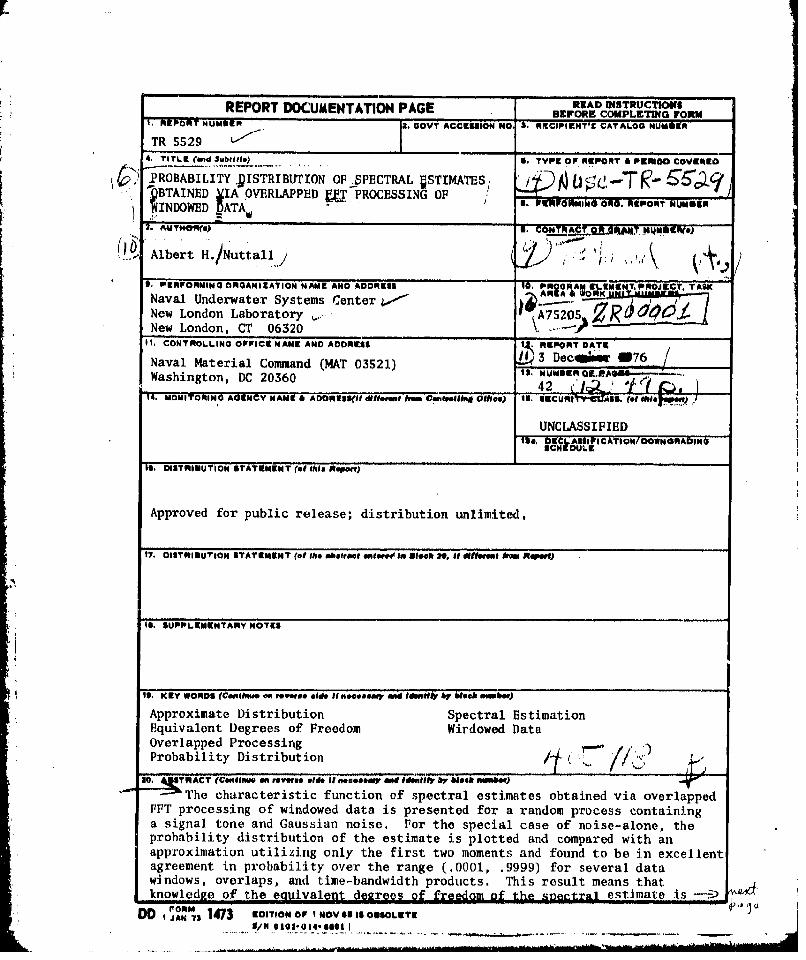
The characteristic function of spectral estimates obtained via overlappedFFT processing of windowed data is presented for a random process containinga signal tone and Gaussian noise, For the special case of noise-alone, theprobability distribution of the estimate is plotted and compared with anapproximation utilizing only the first two moments and found to be in excellentagreement in probability over the range (,0001, .9999) for several datawindows, overlaps, and time-bandwidth products. This result means thatknowledge of the 2guivalent de rees of freemofh scta estimate is -S)

DD I 1473 EDITION OF I NOV 65 IS ONSOLEYE

20. (Cont'd) :c•J•-t adequate for a complete probabilistic description, even when the overlap

results in significant statistical dependence of the component FFT outputs,

TR 5529

TABLE OF CONTENTS

Page

LIST OF ILLUSTRATIONS ...... ..................... ii

LIST OF SYMBOLS .................. ......................... ii

INTRODUCTION ..................... ......................... 1

CHARACTERISTIC FUNCTION FOR SIGNAL PLUS NOISE ...... .......... 2

MEAN AND VARIANCE FOR SIGNAL PLUS NOISE .... ............. . ... 5

PROBABILITY DISTRIBUTION FOR NOISE-ALONE ......... ........... 9

FLUCTUATIONS OF CROSS SPECTRAL ESTIMATE ..... ............. ... 22

DISCUSSION ....................... ........................... 25

APPENDIX A - DERIVATION OF CHARACTERISTIC FUNCTION ......... ... A-1

APPENDIX B - DERIVATION OF COVARIANCE MATRIX .... .......... .. B-1

APPENDIX C - NUMERICAL COMPUTATION OF CUMULATIVE PROBABILITYDISTRIBUTION ............ ................. ... C-1

REFERENCES ..................... ......................... ... R-1

ACCESSION ior

Hill While Sect•i•t 0DCC luif £ocllsb I-Doelot(HUCED 0

JI..... .....................................

IT.... ...............

I .,.. .... .... -.1.1 , ...... ................- .- .,.....

* DtS1H, UZID/AYAIAIInLITY COOEIWt-AV "I.aiuSLtI

• , A

TR 5529

LIST OF ILLIUS'T'RATIONS

"i.gure Pagec

1 Spectral Estimates for Signal Plus Noise ...... ......... 8

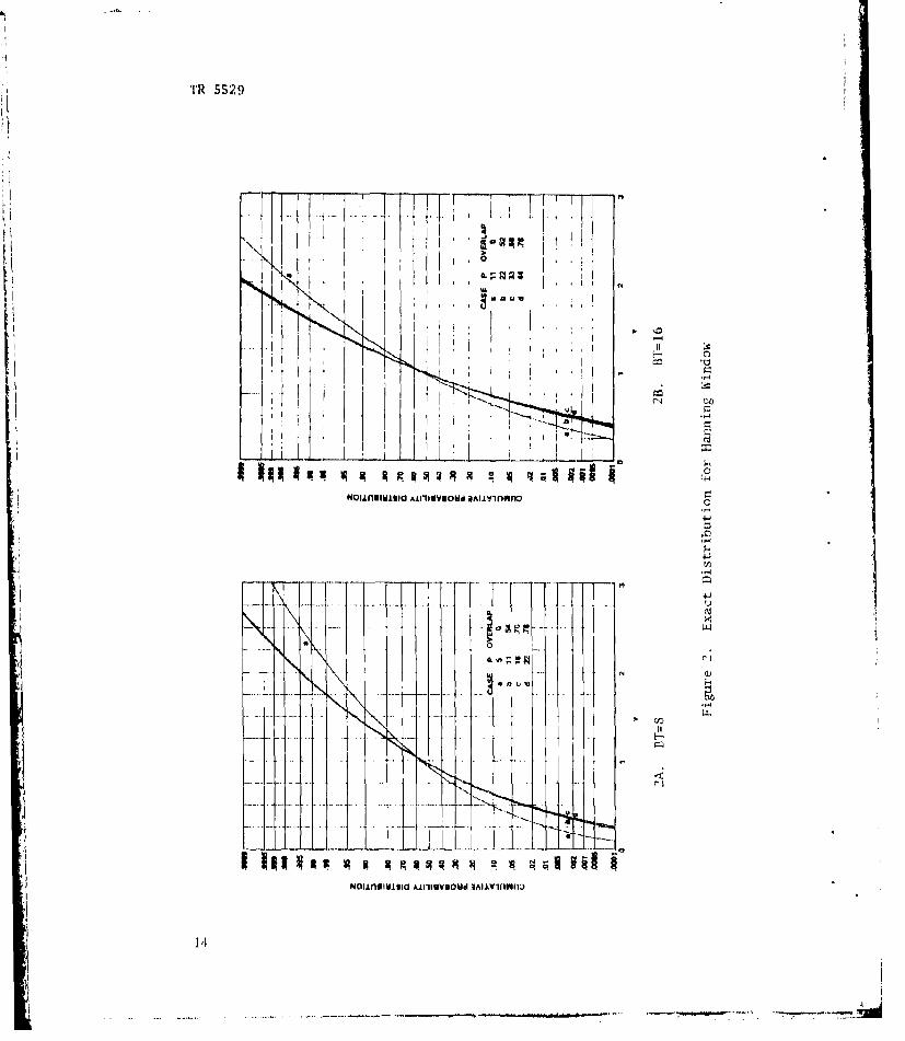
2 Exact Distribution for Ilanning Window ... ........... .... 14

3 Approximation for Ilanning Wi.ndow .o.... . ..... . 16

4 Exact Distribution for Cubic Window ...... ........ 18

5 Approximation for Cubic Window .... ............... ..... 20

JA

j~i

TR 5529

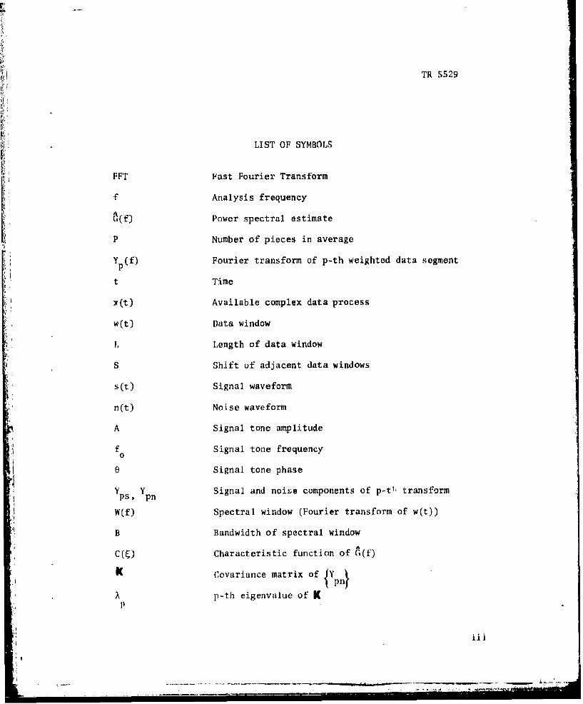
LIST OF SYMBOLS

FFT Fast Fourier Transform

f Analysis frequency

Power spectral estimate

P Number of pieces in average

Yp(f) Fourier transform of p-th weighted data segment

t Time

X(t) Available complex data process

w(t) Data window

L Length of data window

S Shift of adjacent data windows

s(t) Signal waveform

n(t) Noise waveform

A Signal tone amplitude

f Signal tone frequency0

0 Signal tone phase

Yps, Ypn Signal and noise components of p-t 1 , transform

W(f) Spectral window (Fourier transform of w(t))

B Bandwidth of spectral window

C(M) Characteristic function of G(f)

K Covariance matrix of {Yn

pp Sp-th eigenvalue of K

TR 5529

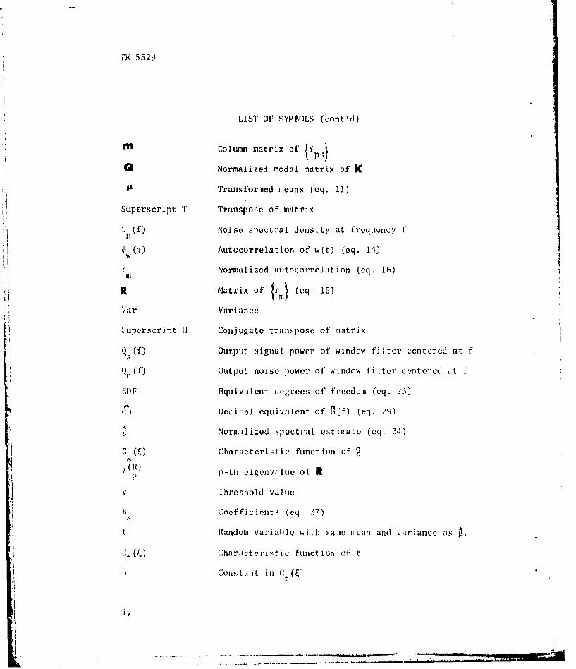
LIST OF SYMBOLS (cont'd)

"m Column matrix of {Y}ps

Q Normalized modal matrix of KA Transformed means (eq, 11)

Superscript T Transpose of matrix

ni (f) Noise spectral density at frequency fn

S(T) Autccorrelation of w(t) (eq, 14)wr Normalized autocorrelation (eq. 16)

R Matrix of r (eq. 15)

Var Variance

Superscript II Conjugate transpose of matrix

Qs(f) Output signal power of window filter centered at fIS

Q1n (f) Output noise power of window filter centered at fIa

Et)F Equivalent degrees of freedom (eq. 25)

t•h Decibel equivalent of I(f) (eq. 29)

A Normalized spectral estimate (eq, 34)

C (M) Characteristic function of *g

A( J p-th eigenvalue of R

v Threshold value

Bk Coefficients (eq. 37)

t Random variable with same mean and variance as .

(4 t(W Charactcristic funct ion of' t

I, Constant in Ct'()

:1 't

iv

TR 5529

LIST OF SYMBOLS (contvd)

K Equivalent degrees of freedom for noise-alone

r Gamma function

IF1 Confluent hypergeometric function

BT Product of analysis bandwidth and available recordlength

Gxy(f), Gxy(f) Cross spectrum and its estimate

A Amplitude of cross spectral estimate

jv

TR 5529

PROBABILITY DISTRIBUTION OF SPECTRAL ESTIMATESOBTAINED VIA OVERLAPPED FFT PROCESSING

OF WINDOWED DATA

INTRODUCTION

Estimation of the autospectrum of a stationary random process by

means of overlapped FFT processing of windowed data (the so-called

direct method) is a popular and efficient method, especially for data

with pure tones present. Stable spectral estimates, as measured by

the equivalent degrees of freedom of the spectral estimate, result

when the product of the available record length and the desired

frequency resolution (the time-bandwidth product) is large in com-

parison with unity. (See, for example, references 1 and 2 and the

references listed therein.)

The equivalent degrees of freedom of the spectral estimate is an

incomplete probabilistic descriptor, because it depends only on the

mean and variance of the random variable. In this report, we address

the problem of obtaining the characteristic function of the spectral

estimate with overlap processingof a signal tone present in Gaussian

noise, and thence the cumulative probability distribution (perhaps by

numerical means as given in references 3 and 4). For the case of

signal-absent also, we will compare the exact probability distribution

with an approximate distribution that uses only the first two moments

of the spectral estimate, to see when the approximate distribution can

7I

TR 5S29

be used as a valid probabilistic description. Some related work is

:Ivailable in reference 5 and the papers cited therein.

A discussion of the relative stability of the spectral estimates

with signal tones present, and of a cross-spectral estimate,completes

the presentation.

CHARACTERISTIC FUNCTION FOR SIGNAL PLUS NOISE

The method and conditions of processing are described fully in

reference 1 and, for sake of brevity, will not be repeated here. The

•power spectral estimate at analysis frequency, f, is given by

(reference 1, pp. 2-4)

G(f) - p ,2 ly (f)J)

p=l

where P is the total number of weighted data segments. Hlere*

Yp(f) = dt exp(-i21Tft) x(t) w I L - (p-1) , (2)

where x(t) is the available (complex) data process, W(t) is the data

window of length L, and S is the amount of shift each adjacent data

window undergoes. The fractional overlap is therefore 1 - S/IL.

*Integrals without limits aIrc over the range. o) non-zero integrand.

Best Available Cor'"

TR 5529

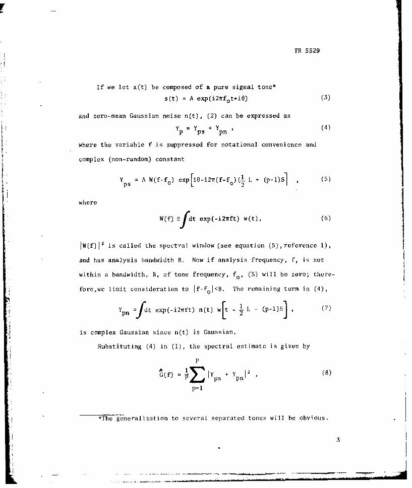
If we let x(t) be composed of a pure signal tone*

s(t) = A exp(i2wfot+iO) (3)

and zero-mean Gaussian noise n(t), (2) can be expressed as

Yp =Y + Y (4)p ps pn

where the variable f is suppressed for notational convenience and

complex (non-random) constant

Yps A W(f-fo) exp r-i27(f-f O)( L +

where

W(f) =fdt exp(-i2lrft) w(t). (6•)

IW(f)1 2 i.s called the spectral window (see equation (5),reference 1),

and has analysis bandwidth B. Now if analysis frequency, f, is not

within a bandwidth, B, of tone frequency, f., (5) will be zero; there-

fore,wc limit consideration to if-.fo1<B. The remaining term in (4),

Yp jdt exp(-i2nft) n(t) w t - (P-I) S (7)

is complex Gaussian since n(t) is Gaussian,

Substituting (4) in (1), the spectral estimate is given by

A 1 2 (8)11E) j ps +IYp5 +

p=l

*The generalization to several separated tones will be obvious.

3

TR 5529

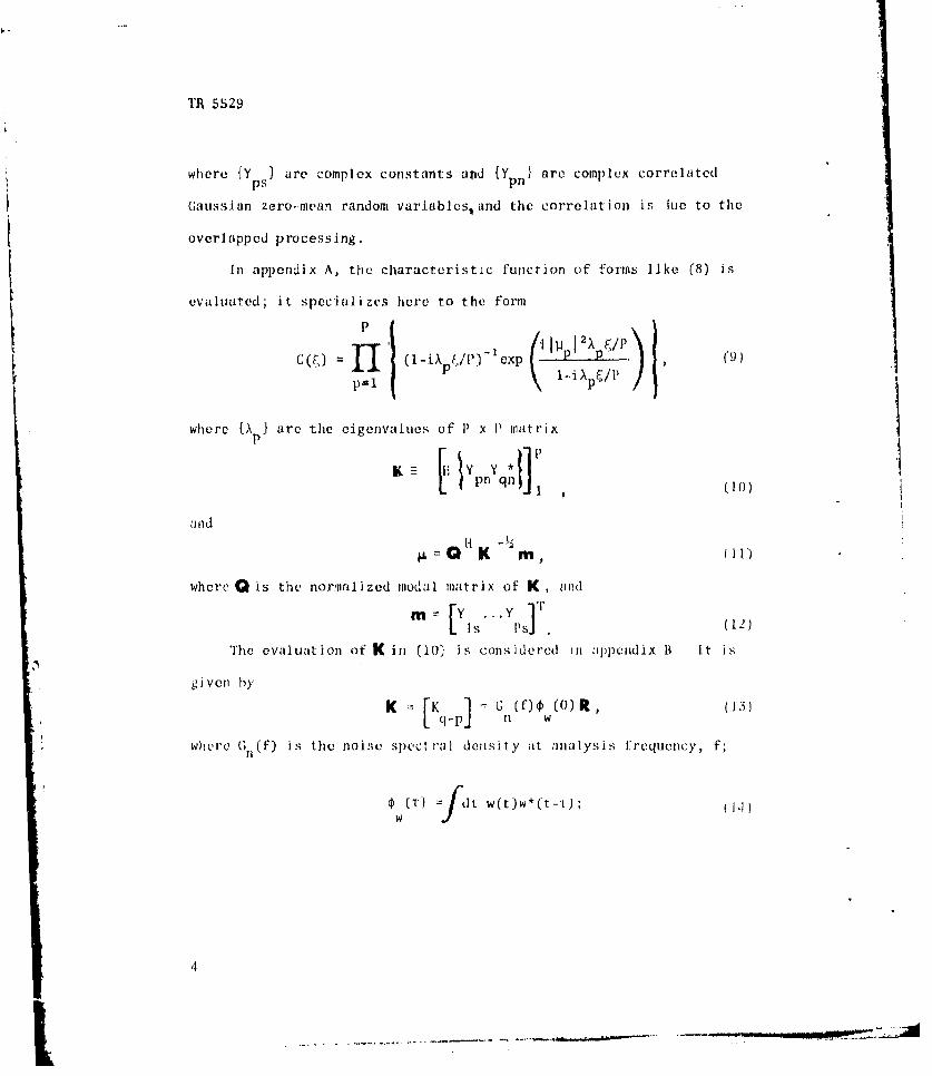
where {Y ps are complex constants and Y pn) are complex correlated

Gaussian zero-mean random variablesand the correlation is Wue to the

overlapped processing.

In appendix A, the characteristic function of forms like (8) is

evaluated; it specializes here to the form

C(:) UP ()iXpJ exp [ (9)

where (PA are the cigenvalues of1 P x P matrix

K - pnqj 1 ,(10)

and

0--Q K m

where Q is the normalized modal matrix of K, and

Is' , , . (12)

The evaluation of K in (10) is considered in ;ippendix B It is

given by

K - n (f)G w (0) R, (13)

where G 1(f) is the noise spectral density at analysis frequency, f;

w ) - t w (t)W * Ct-4)

TR 5529

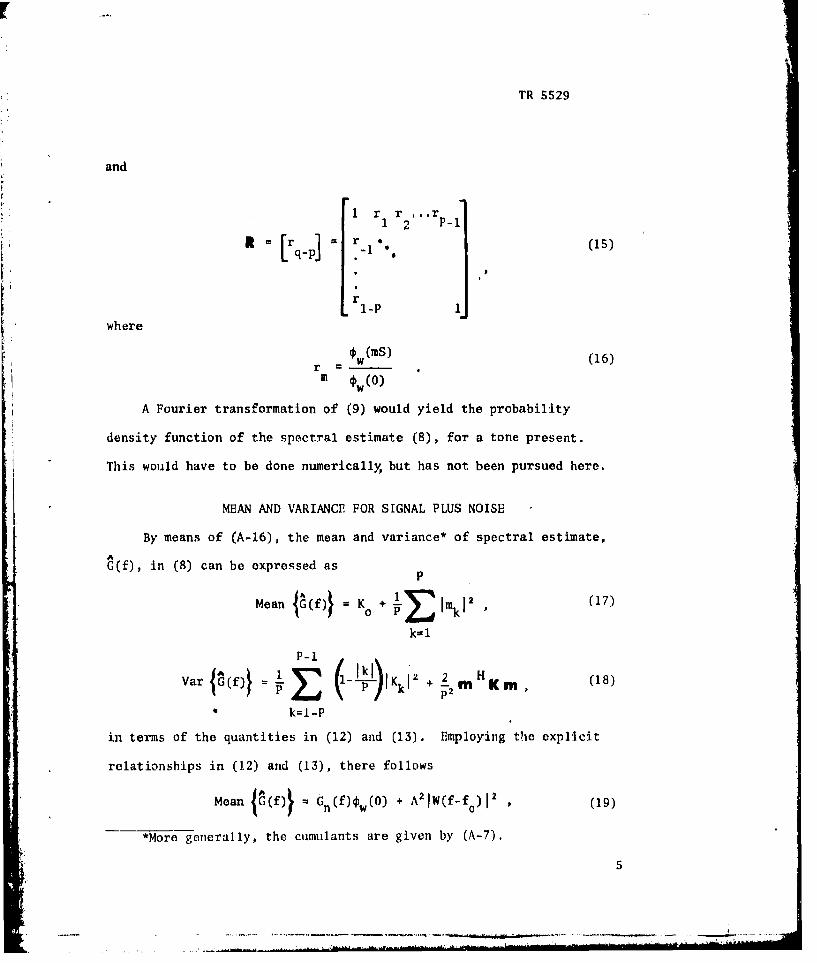
and

1 r r ... r12 p-i

R [q-]

r1-P 1

where

r = (is) (16)r = -m ýW (0)

A Fourier transformation of (9) would yield the probability

density function of the spectral estimate (8), for a tone present.

This would have to be done numerically, but has not been pursued here.

MEAN AND VARIANCE FOR SIGNAL PLUS NOISE

By means of (A-16), the mean and variance* of spectral estimate,AG(f), in (8) can be expressed as

Mea K~f c + .1 3~ (17)

k=l

P-1

Var G(f) P " VKk1' + 2M Km (18)

"k=l-P

in terms of the quantities in (12) and (13). Employing the explicit

relationships in (12) and (13), there follows

Mean {((f) = Gn(f)ýw(0) + A2 IW(f-fO)l 2 (19)

*More generally, the cumulants are given by (A-7).

r5

TR 5529

and

H ~~Var G =f LM ý (t) 0o]~ i.4)Ik

2A 2 1 W~f-f 2G 11 Mý(O~rl k=E1(- Ik P x i2nff

k=l-P

where we have employed (15) and (S).

At this point, it is conVenient to def'I ine the output signal power

of a window filter with transfer function, W, centered at f as

Q .; ( f ) -- A 2 1 W ( f -f o 0 ) 1 2 , : , ),

and the output noise power of the stnie filter Lis

'T'hen (.19) and (20) take the forms

Mean ((f) Qn:(f) + QSf) (23)

Var {2(f = Q2(f i ( Irk '

n 1) AE k )Ikk=l-l"

+2Q E ( i ... rk exp(ik211(f-fo)S) (+2s (f kn 0t g (2 ,1)

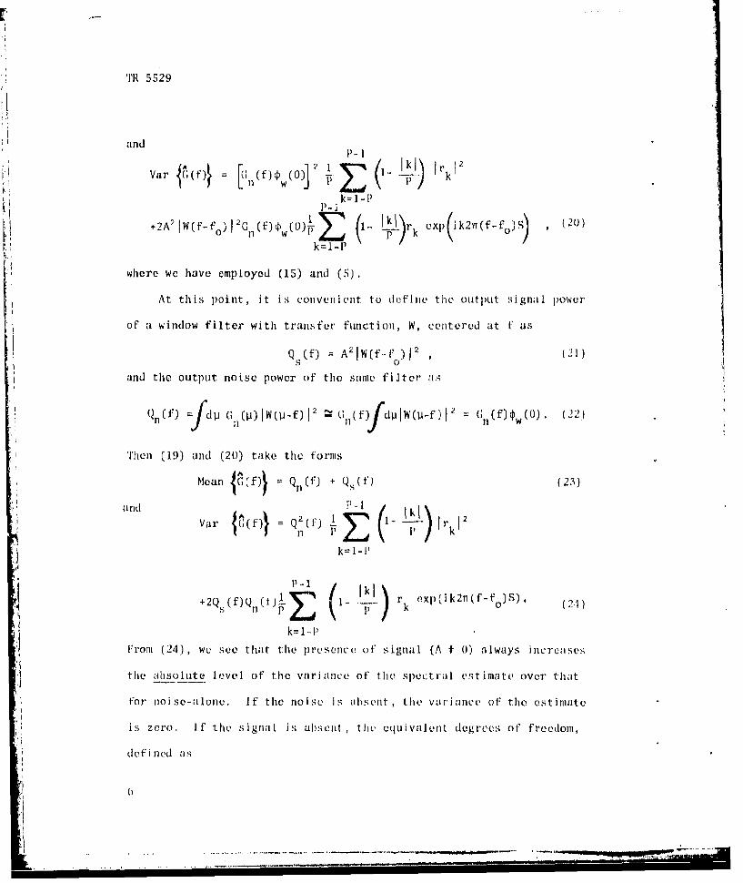
k=l-PFrom (24), we see that the presence of signal (A f 0) always increases

the absolute level of the variance of the spectr al estimate over that

for no ise-alone. If the noise is absent, the variance of the estimate

is zero. If the signal .is absent, the equivalent degrees of freedom,

defi ned as

.10

TR 5529

2 (Mean) 2 2EDP E (25)

n Variance P-1

k-l-P

is identical ito equation (8), reference 1, as it should be.

On the other hand, for Qs(f) " Qn(f),

EDF 2(Mean) 2 9s (26)s Variance / -, (26)

Q (f) 1 -( )rk exp(ik2Tr(f-fo)S)

k=l-P

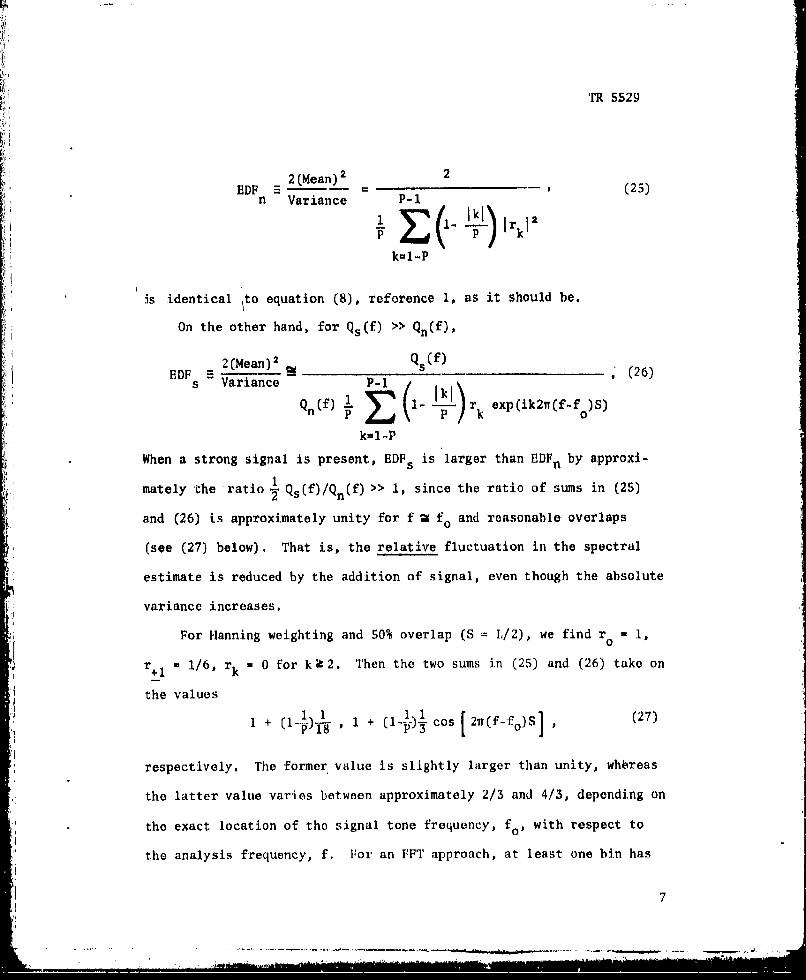
When a strong signal is present, EDFs is larger than EDFn by approxi-

1mately -the ratio ( s (f) >> 1, since the ratio of sums in (25)

and (26) is approximately unity for f a fo and reasonable overlaps

(see (27) below). That is, the relative fluctuation in the spectral

estimate is reduced by the addition of signal, even though the absolute

variance increases.

For Hanning weighting and 50% overlap (S = L/2), we find r - 1,

r+1 = 1/6, rk = 0 for k t2. Then the two sums in (25) and (26) take on

the values1+ •1 1 [ ] (27)

1 +I -) ,1 + (l-1C-) S Cos 2 T(f-fo)S ,

respectively, The former value is slightly larger than unity, whkreas

the latter value varies between approximately 2/3 and 4/3, depending on

the exact location of the signal tone frequency, f., with respect to

the analysis frequency, f. For an FFT approach, at least one bin has

7

.. . .--.-- - -. . . . . . . . . -.----.-.- ,L-

T'I 5529

its frequency location, f, such that If-foIt (21,Jf 1 ; thus, at least

one frequency bin is located such that the latter value in (27) is

larger than unity.

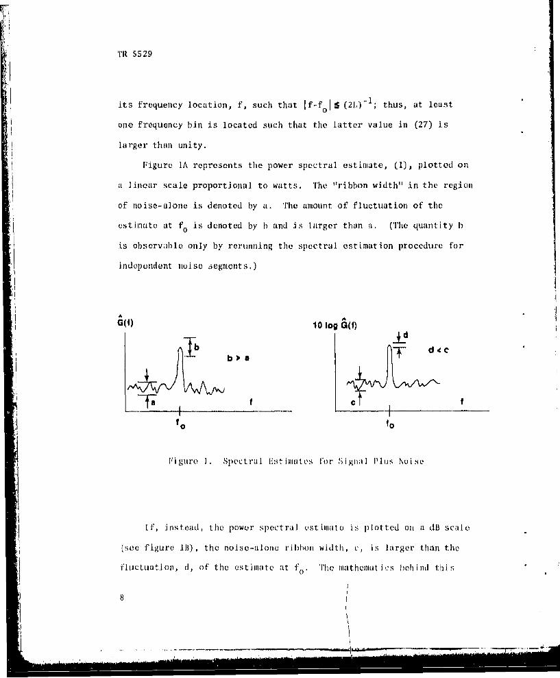
Figure 1A represents the power spectral estimate, (1), plotted on

a linear scale proportional to watts. The "ribbon width" in the region

of noise-alone is denoted by a. The amount of fluctuation of the

estimate at f0 is denoted by b and is larger than a. (The quantity 1

is observable only by rerunning the spectral estimation procedure for

independent noise iegmcnts.)

G(f) 10 log G(f)

.1b T d .cci b> a

fo ýoo

-~~ f _-

ligure 1. Spectral lHtkimatcs for Signal I i.,'s Noise

If, instead, the power spectral esti,•ate is plotted on a dB scale

(s o e figure I), the noise-alone ribbho, width, c, is larger than the

fluctuati on, d, of the estimate at f The mn1athelllt itjs behind thlis

* ,, -. ' , ___.- --

TR 5529

conclusion follows. Let the spectral estimate at frequency f be

expressed as

S(f)= x, (28)

where m is non-random and x has zero-mean and variance a 2 , Then

E 10 log G(f) = 10 log m + 10 log(l+XS), (29)m

Now suppose that o/m<<1, which could be realized by means of a large

number of pieces, P, or a high signal to noise ratio; then

AI2I0 log m+ in 10 o x (30)

The last term in (30) is proportional to the relative stability of the

spectral estimate (28); in fact

Var (d a 1710/2 .2 (1

which can be made arbitrarily small. Thus a plot like figure 1 is

easily achievable and should be anticipated for a pure tone in Gaussian

noise.

PROBABILITY DISTRIBUTION FOR NOISE-ALONEA

For noise-alone, the mean and variance of spectral estimate, G(f),

are available from (19), (20), and (16) as

Mean {•(f) Gn(f)4ýw(O),

P-I

Var {G(f)} = GE(f) ( ( 1-k Ib(kS)I 2 (32)

k=I-P

! 9

TR 5529

which agree with equations (5) and (6), reference 1, respectively.

More generally, tile characteristic function follows from (9) as

pr-

Now lot us define a normalized random variableA(;f

GA n (' w7) (

notice that tile scale factor is independent of P) and the amount of

overlap, Thus the mean li{f) 1, and thu characteristic function or

.15'cg C() = [ I-i'tR/ij (35)

where tX are the eigenvalues of matrix R in (15) . Then by a

partial fraction expansion, the probability that random variable

remains below a threshold value, v, is found to be

Prob (9,<v) = B 1lk Oxl (, v>O, (30)

13 k 1 k :5' (37)1

k pk

pIk

TR 5529

We have assumed all the eigenvalues of Rto be unequal; this is the

case if the overlap is greater than 0, which is the case of most

practical interest. The eigenvalues are all non-r .. 'ative since R is

a non-negative definite matrix (see appendix B).

Equation (36) is an exact expression for the cumulative probability

distribution in terms of the eigenvalues of matrix R. If we consider

another random variable, t, with the same mean and variance as g, a

candidate approximate characteristic function is (guided by form (35))

Ct(•)= (l-iC/b)"b, (38)t

where, in order to maintain the same variance, we choosep P P-1

(R) 2 2•Xp - (- 2 (i)rk39)

pMl p,q=- k-l-P

Equatior (8), reference 1, shows that b = K/2, i.e., half of the

equivalent degrees of freedom, Then the approximate probability

density function is

1 bbb-l -btp(t) - - b t e , t>O, (40)

r(b)

and the approximate cumulative probability distribution is (equations

6,5.2 and 6.5.12, reference 6):

t p(t) (bv)ebv (1;i+b;bv), v>O. (41)

"!<J P(b+l) 1 1

0

............

11

TA~ 5529

(A further simpler approximation, not piirsuced here, would lie to set

bi= integer part of b, b 2 = 1)1 + I., and bracket the results above by

two simpler sums.)

We shall now make quantitative comparisons between exact -result

(36) and approximation (41) which hus the same mean and variance. The

question is: is b in (39) and (41) a1 SUffliCient statistic to accurately

quantitatively describe the exact cumulative probability distribution

(36), for representative data windows, over' ap, nlumberC Of pie-ces, and

time-bandwidth products, over th! ranlgO Of prlobabilitieS, Of interest

*to most uscr.,i? r1 so5, then atf-L-nt ion can be confined to thle equiva lent

:1 degrees of freedom and Its maxinhizat ion alone, as was done in reference

1; this simplification would be most worthwhile and of obvious iimpor-'

tanice.

The actual numerical computation of' tho cumulativoe probabil11ty

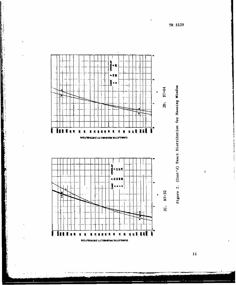
distribution Prob(&1-v), is considered in appendix C. In fi gur'e 2, the

exact cumulative probability distribut ion for lianning windowing is

presented for t inc-bandwidth product BT' = 83, 16, 3-2, 04, where TI is

the available record length and 13 is the des ired resolut ion bandwidth.

In each plot, the overlap is varied from 0I to appr'oxi mately 75', and

the di stribut ion plotted on a normalI probability ordinate covering tile

range (.0001, .9999) . The fact that the curves are not straight lines,

aver this range means that a (Jaussi an approx i at ion to thle power,

spectr'al estimate would not sutffice. However , the Gauss ian approximaa-

tion would be a fairly good one for larger BT1 and 11 (see figure 21), for

example),

12

TR 5529

The fact that the curves in figure 2 are-virtually identical for

overlaps greater than 50% means that there is little point in choosing

overlaps greater than this amount. This confirms the choices of over-

lap made in reference 1, where attention was confined to the equivalent

degrees of freedom, The ideal distribution would be a vertical line

at v = li the closeness of these curves to the ideal is a measure of

the spread of the spectral es-Jimate.

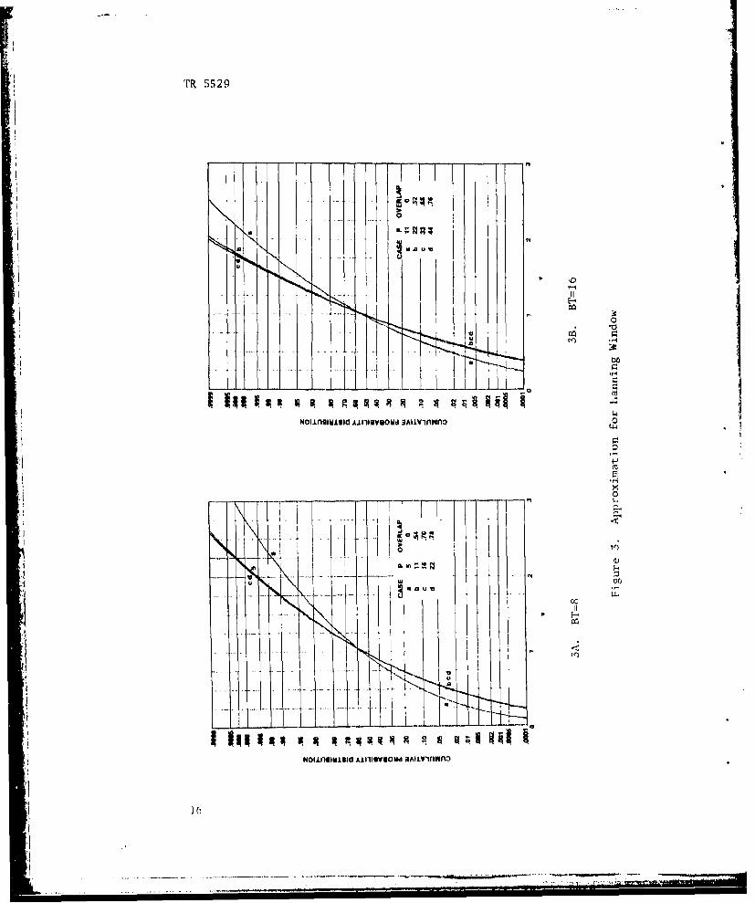
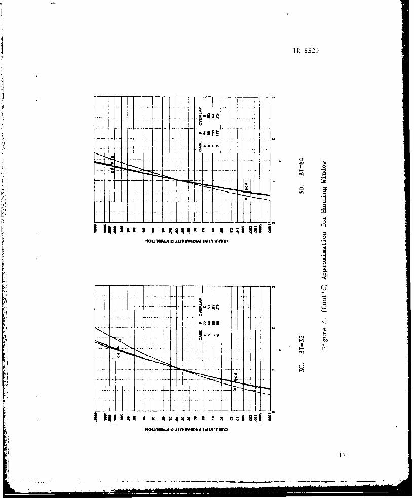
The corresponding results for the approximation (41) are presented

in figure 3. The curves are virtually identical to those of figure 2

over the complete range of probabilities considered, for various values

of BT and overlap.

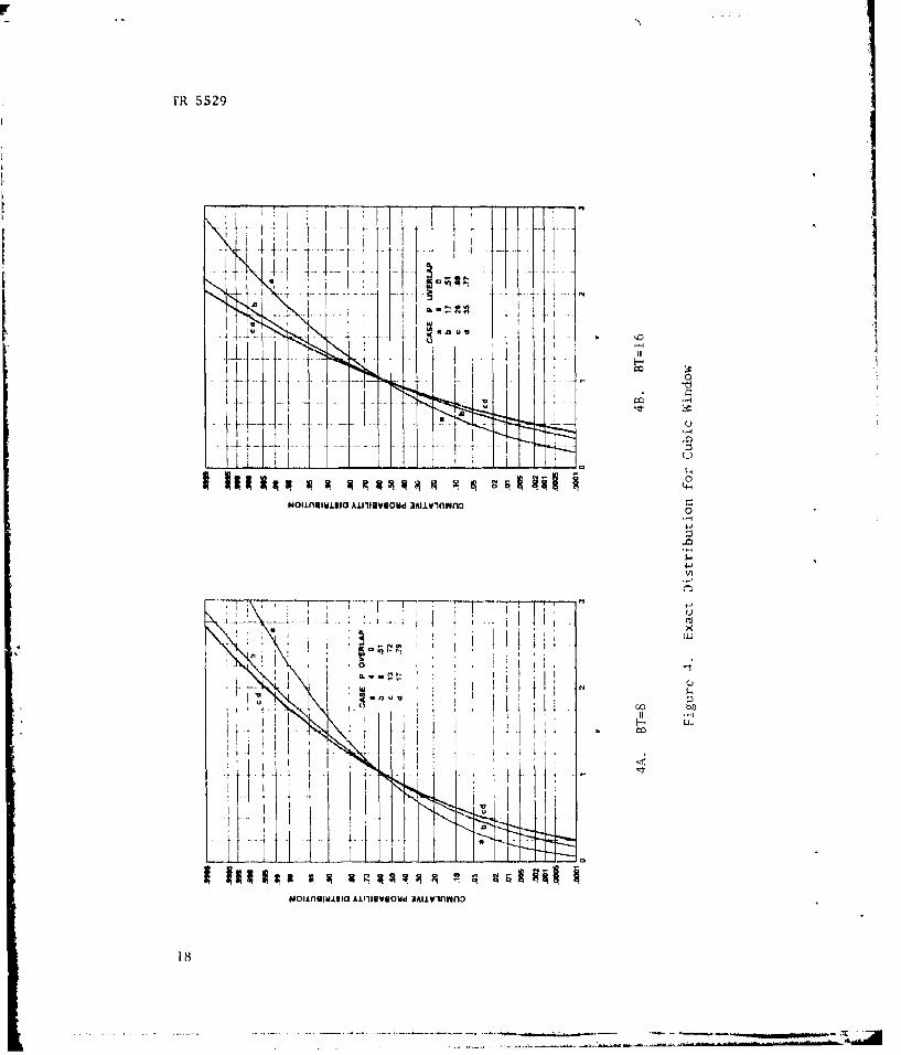
For a cubic window, the exact results and the approximation are

given in figures 4 and 5, respectively, The conclusions are identical

to those made for the Hanning window.

I.

j 13

"-"- - -

•1 •-

TR 5529

R1 m I i

H 0

I4-

Nonii~aAllgBlt ~ lvnn

TR 5529

0

q 0Iu

OI N

q 00

4 *4~L;

NounW111 AilIM4hM DI.Lvnon

'FR 5529

D- A~ 4

a A u '

0

..1 .Ii II c

ILI

101

houflhlimilO A.LIIIUVUOMd MmAiLWmfnf

'FR 5529

II 0

td'

IL cu04

I ~ ~ o0.L

NoIfuniM1110 AJillguVSod NAI±~lvnono

17

Wim

TR 5529

IL H

'A

p +4

.2---------------------' II T I*'~ ~#

Woi. owl Iilvo~ I*iinn

V TR 5529

IT,

co~ -4

4t4

FT0

-oniii Awovo Ma.4n

I IRER~! q q qq~qq 19

'I'l 5S2 9

0I

LL Kr~'r-- ]~

-7 1)T

NounITflIIuO AILI~IUY9OOd 3IAviLnnno

20.

TR 5529

_ r4

0

G149

01

Ii 'Ii 4 4 k

21

TR 5529

F ILJCTUATI ONS OF CROSS SPECIRAIL ESTIMATE.i

This topic ls not directly related to the earlier material on

aUtospectral est.i.mation; however, it :is an important observation and

merits a commnent. For two uncorrelm ted processes, x and y, the cross

spectrum G (f) 0 . However, the cross spct ral est I In;ItC 0 (M)xy xy

sat 1.sf los the equat ions (reference 2):

S1,

1 C f 12 = 2 , (f)(; (.) (42)xy - x yy

whel'iC K is thie equivaltent degrcee; of' C, v )dom, Now, i F K>> I, C (F) isxy

approxiumately Comp lex Cau';ssian. Therefore, itf we deflne tho amplitude

cst~imate

A r ( t') l (43)

it has prolab i lity density funct ltor

x) exp ..... x>O , 4(72()X1

Then the mean oF A Is

I: f~' (1 G ( f) (ý J (45)K /

which is a rather slow decay with K. Then thu ratio of the moian

a1mplitude, (45) to the Square root of the product 01' the autto-spectra

22

TA 5529

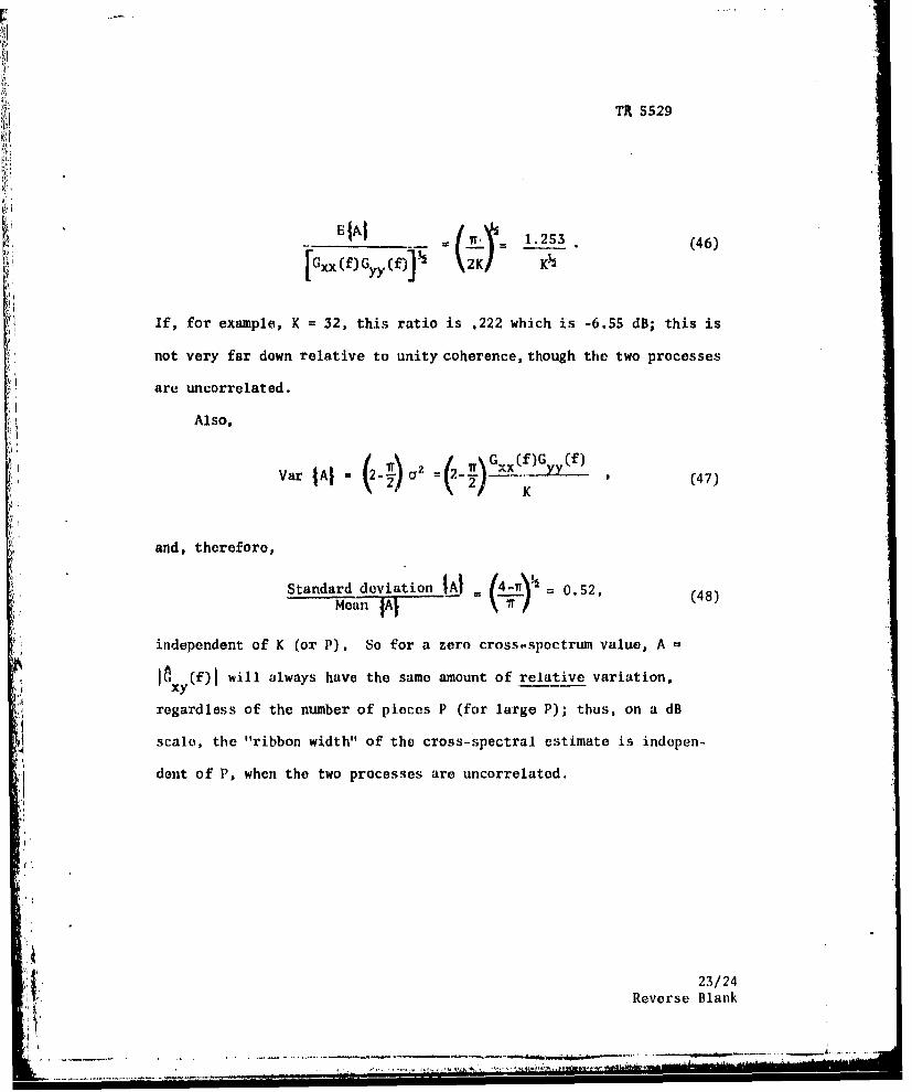
_________ _ 1.2._•53 (46)[Gxx Mf Gyy (f)l 1 TK½

If, for example, K = 32, this ratio is .222 which is -6,55 dB; this is

not very far down relative to unity coherence, though the two processes

are uncorrelated.

Also,

Var JA (2 -E) C2 (4-7) K~)G~f (47)

and, therefore,

Standard deviation -AI (- w.)½= 0.52, (48)Mean JII

independent of K (or P). So for a zero cross-spectrum value, A

] xy(f)l will always have the same amount of relative variation,

regardless of the number of pieces P (for large P); thus, on a dB

scale, the "ribbon width" of the cross-spectral estimate is indepen-

dent of P, when the two processes are uncorrelated.

23/24" Reverse Blank

I II

TR 5529

DISCUSSION

An exact expression for the characteristic function of the power

spectral estimate of a pure tone in Gaussian noise has been attained,

and then specialized to noise-alone, In the noise-alone case, a

numerical computation of the cumulative distribution function has been

conducted. Comparison of the latter with an approximation utilizing

only the mean and variance shows excellent agreement over a wide range

of probabilities, regardless of the exact window, overlap, or the time-

bandwidth product. This means that concentration on the equivalent

degrees of freedom, particularly on its maximization, is sufficient

for a probabilistic description of the auto-spectral estimate,.

Maximizing the equivalent degrees of freedom results in a narrower

probability density function, as witnessed by the increased steepness

of the cumulative probability distributions presented.

An entirely different method of auto- and cross-spectral estimation

has been presented in references 7 and 8, and is mentioned here as a

viable, attractive alternative, particularly for short data segments.

Since only a few parameters are estimated, the estimates are potentially

more stable, whereas the technique considered here (and in reference 1)

assigns independent degrees of freedom to each and every frequency

cell of interest and, therefore, requires the estimation of many more

parameters.

25/26Reverse Blank

TR 5529

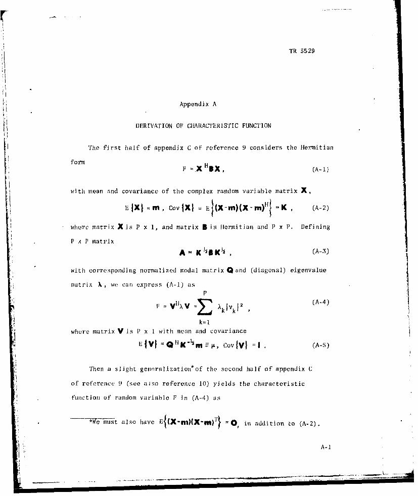
Appendix A

DERIVATION OF CIIARACTEIRISTIC FUNCTION

The first half of appendix C of reference 9 considers the Hlermitian

form

F =.X HBX (A-1)

with mean and covariancc of the complex random variable matrix X,

n 1Im, Cov 1Ix =F t(x-n)(X- m)" K (A-2

where matrix Xis P x 1, and matrix B is Hermitian and P x P. Defining

P x 1 matrix

Au K BK (A-5)

with corresponding normalized modal matrix Q and (diagonal) eigenvalue

matrix X., we can express (A-i) asP

F = V~xv E )•kVka(A-.4)

k=l1where matrix V Js P x 1 with mean and covariance

EIVI = Q "K½m K-I , Cov{V} :I (A-s)

Then a slight generalization*of the second half of appendix C

of reference 9 (see also reference 10) yields the characteristic

function of random variable F in (A-4) as

*We must also have in addition to (A-2).

"A-1

S..... .. ...... .... .--.. - i -- • •.... . . .

-p iItk 2xkj

(exp (A-(6)

k=1

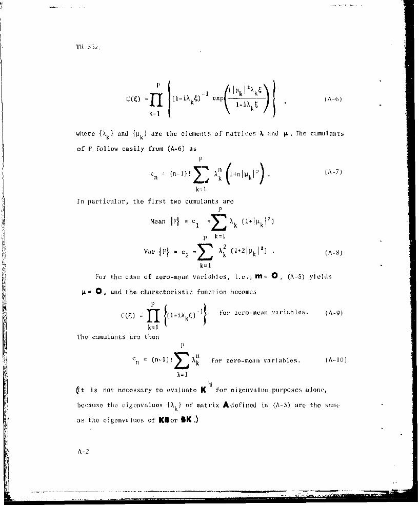
where {Xk} and (IpkJ are the elements of matrices X and g. The cumulants

of F follow easily from (A-6) as

( n-I)! (+nipij~ (A-7)

k=l

In particular, the first two cumulants arc

i Mean 1JF = Cx (I+Ilk•)

p k=1E' 2 (l+21pkI')

Var 1'= C 2 -- k )1.2 .(A-8)

k=l

For the case of zero-mean variables, i..e. ,m 0, (A-5) yields

0, and the characteristic function hecomes

J[ 1 (l-iAkgV- for zero-mean variables. (A-9)

k= 1The cumulants are then

nC = (n-l)••n ) k for zero-mean variables. (A-I)

k=1

Ot is not necessary to evaluate K for Cigenvalue purposes alone,

because the eigenvalues {AkI of matrix Adefi ned in (A-3) are the salwl(

as the cigenva lues of Klor SK,)

A-2

ij1

'TR 5529

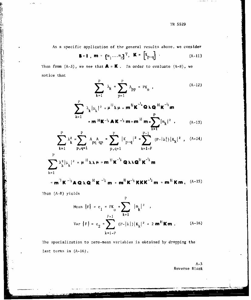
As a specific application of the general results above, we consider

B = I , m I K = [Kp_ (A-11)

Then from (A-3), we see that A = K . In order to evaluate (A-8), we

notice that

P 1) (A-12)k AkZ= App =PKo

k=l p=l

Fa AK kQkXQ HK-ýIm

PP

--m HK AK ~'m=m Hm= m~ (A-13)

I P I P-i1

2 W 2= AIXXJA= M 11 K-A-X14"KJ.'

A2 = ApAq = .Kpq =Z (P-Ik1)IKk1

k=l p,q=l p,q=l k1l-P

=Ah k I 11 HK- Q X, Ql K-m

k k

k=l'! ~~~K -M- H kH-s MH (A-S

-m 'K AQ Q K " m K-1 KKK m - Kin,

'Then (A-8) yieldsP

iMean 1F} C= PK + in'k ,

P-1 k= I

Var = c2 =E (I[Ikl)IKk + 2 mH Km. (A-16)

Sk=1-1P

,The specialization to -ero-mean variables is obtained by dropping the

last ternis in (A-16).

A-Reverse Blank

TR 5529

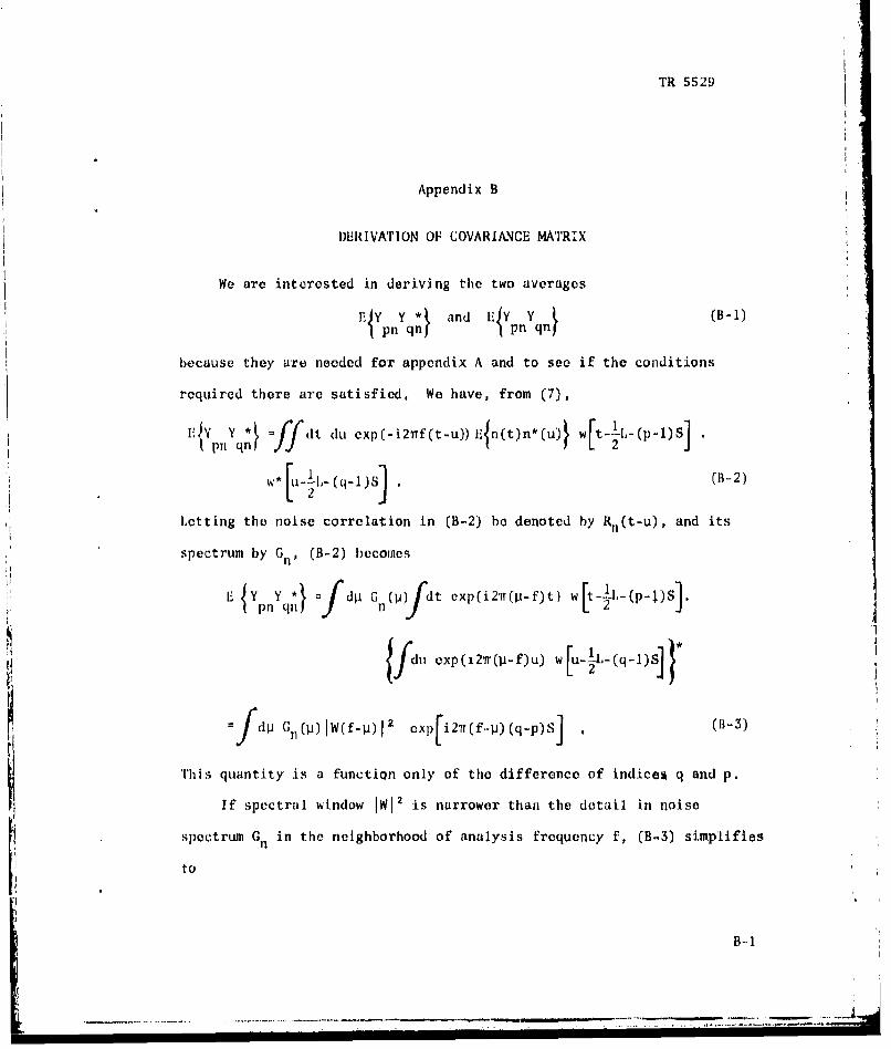
Appendix B

DERIVATION OF COVARIANCE MATRIX

We are interested in deriving the two averages

r~Yp~Yq~and EYf~~ Bi

because they are needed for appendix A and to see if the conditions

required there are satisfied, We have, from (7),

I.-p,'~ Y =ff (t du cx,,-i 2,Tf (t -u)) E n(t).• ,,*--,-(u)s]

w* l(B-2)

Letting the noise correlation in (8-2) be denoted by Rn(t-u), and its

spectrum by Gn, (B-2) becomes

E jYpnYjYq =fdp Gn(IJfdt exp(i21T(IJ-f)t) w[t-l-(p-1)SJ

fu exp(12ir(.p-f)u) w - ,-(q-l)

'ýSdji C(1j)1"W(f")12 eXP i27r(f-jj)(q-p)S] (B-3)

This quantity is a function only of the difference of indices q and p.

If spectral window lwla is narrower than the detail in noise

spectrum Gn in the neighborhood of analysis frequency f, (B-3) simplifies

to

B--1

_______ -- .. - -.-- , . ----.- -a-- - -.- -..- .

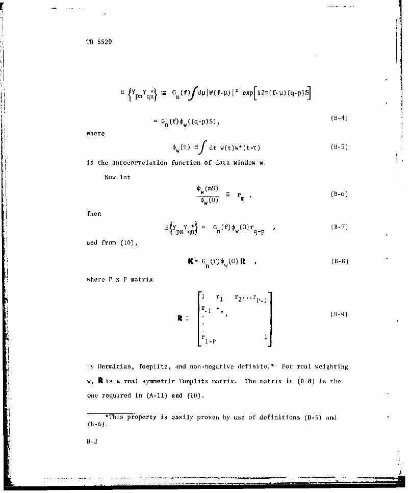
TR 5529

E {plq (f jfdvAW (f -p)i2 exp[i2Trf-Iv q-ps]

- Gn (f) w ((q-p)S), (13-4)

whereýw (T) fdt w~t)w*(t-T) (B-5)

is the autocorrelation function of data window w.

Now let

-r , (8-6)Ow {0S) r

Then

E13YpfnYqn n = Gn(f)w (O)rq-p (B-7)

and from (10),

K= G n(f)c1(O)R , (0-8)

where P x P matrix

"I rI r 2 .. ,r

ri

r 1

is IHermitian, Toeplitz, and non.-negatlvo definite.* For real weighting

w, Rlis a real symmetric Toeplitz matrix. The matrix in (1-8) is the

one required in (A-11) and (10).

*Trhis p-operty is easily proven by use of definitions (B-S) and({3-6).

B-2

.. .. .. ..

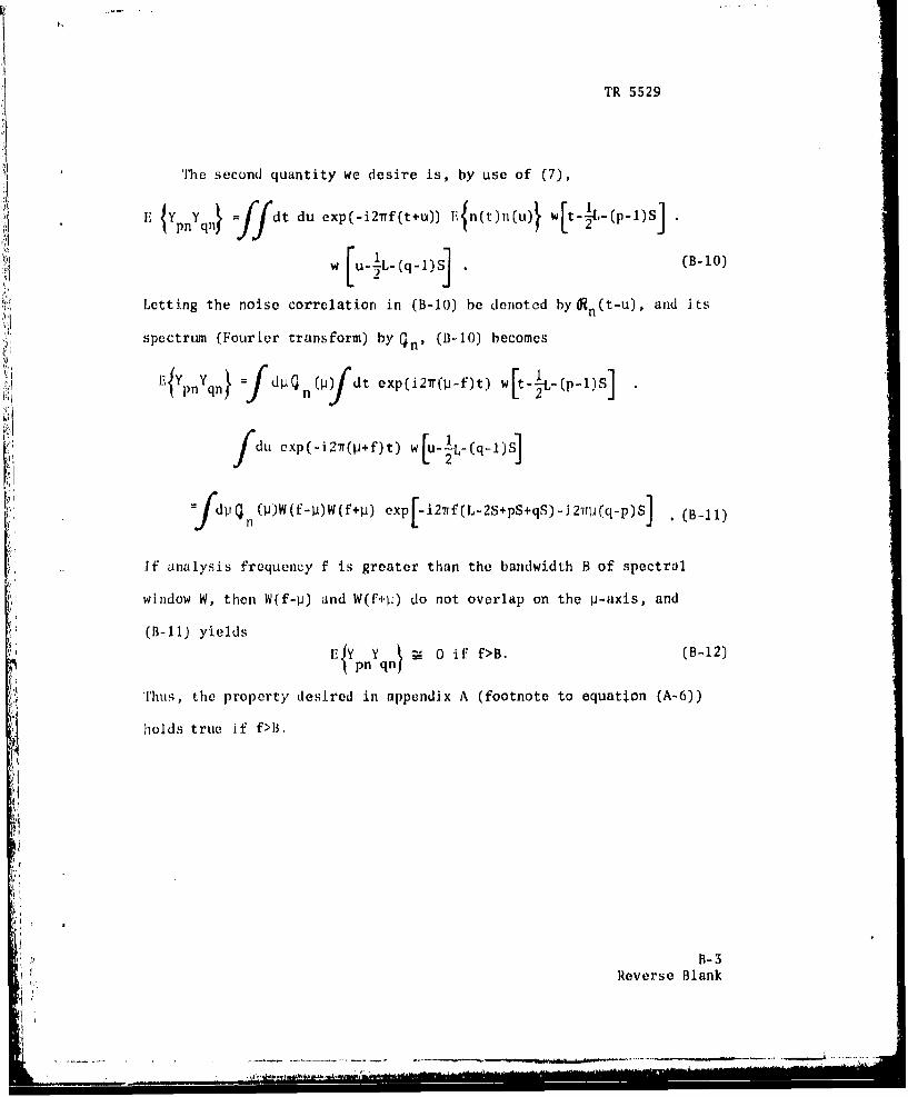
TR 5529

The second quantity we desire is, by use of (7),

Y {YpnYqnl =fdt du exp(-i2wf(t+u)) F{n(t)n(u)ý w[t-2 -(P-)S],

w [uIL.(q.1)S (B-10)

Letting the noise correlation in (B-10) be denoted by On(t-u), and its

spectrum (Fourier transform) by Gn. (B-1O) becomes

E-{YpnYqn)} =Jdpn G( dt exp(i27r(wl-f)t) -L-(p-1)S

(p) Q W(t-1i)W(f+11) C .(Bil

If analysis frequency f is greater than the bandwidth B of spectral

window W, then W(f-p) and W(f+s.) do not overlap on the p-axis, and

(B-11) yields

E3YpnYqn, ý 0 if f>B. (B-12)

Thus, the property desired in appendix A (footnote to equation (A-6))

holds true if f>B,

.A

ti'B3-3

Reverse Blank

- 4 .

TR 5529

Appendix C

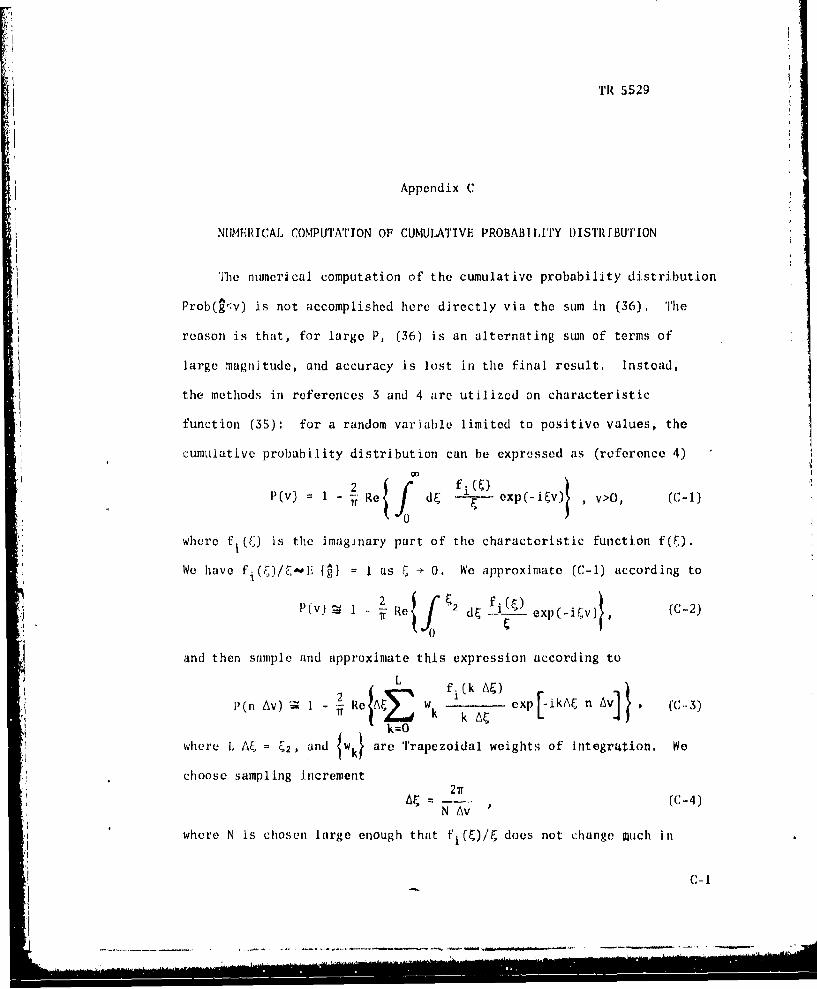
NUMERICAL COMPUTATION OF CUMULATIVE PROBABIIraTY DISTRIBUTION

The nunerical computation of the cumulative probability distribution

Prob(*<v) is not accomplished here directly via the stun in (36). The

reason is that, for large P, (36) is an alternating sun of terms of

large magnitude, and accuracy is lost in the final result. Instead,

the methods in references 3 and 4 are utilized on characteristic

function (35): for a random variable limited to positive values, the

cumulative probability distribution can be expressed as (reference 4)

P(v) = 1 - Re d -- oxp(-iv), v>O, (C-1)

where F is the imaginary part of the characteristic function f(Q).

We have fi(9)/lii {•} 1 as 0 + 0. We approximate (C-i) according to

P(v) T Ile dý .i_ exp(-itv)

and then sample and approximate this expression according to

L f.(k AQ)1

l)(n Av) -M - R Re {A Wk exp I[kAC n A , (C-3)

k=Owhere L At - C2, and w are Trapezoidal weights of integration. We

choose sampling increment21r

N• - , (C-4)N Av

where N is chosen large enough that fi(ý)/F, does not change m4uch in

S~C-I

TR 5529

AF. Then

P(n Av) I Le f1(k w A71nTr k k Aýk=O

N-1

2 AE Ile~ exp[.i27rkn/N (c -5)

k--Owhere

g W .fi((k+jN) At,)k k+jN (k+jN) A&j :

SI. + i 1 I, A . I, 1 ( -0 5k :5N-1, -N N

l~quat 10n (C-5) .s an N-poi.nt FFFT; therefore, we choose N as a power of 2

for speed purposes.

The only remaining quest ion is the choice of I imit • in (C-2)

From (35) , we know that

f f____ ((:-7)

pSmax {1, rp•

p=l

where rp x ( 11)/. Therefore

p~ p

PP

1If" ( ,)1 I -,(: •1 P

p=I 1P

C-2

I~ -~

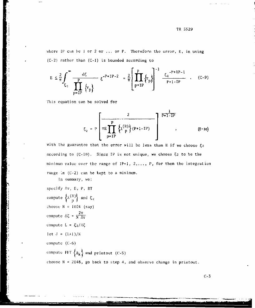
TR 5529

where II can he I or 2 or .. or P. Therefore the error, E, in using

(C-2) rather than (C-I) is bounded according to

00 - P + I P- Ihi dC ______ -P+IP-2 2 jrý(C-9)

P+I-IP

p=IP

This equation can be solved for

1

[ 2 1) p+-ip

p=IP

with the guarantee that the error will be less than Ei if we choose ý2

according to (C-10). Since 1P is not unique, we choose 2. to be the

minimum value over the range of IP=I, 2,..., P, for then the integration

range in (C-2) can be kept to a minimum.

In summary, we:

specify Av, E, P, BT

compute X(R)t andIp ý

choose N = 1024 (say)

2'ir"compute N-T--

.: ~~comipute L = ./,

let .J r (1,+I)/N

compute ((-6)

compute FI'T {igk} and printout (C-5)

choose N 2048, go back to step 4, and observe change in printout.

C-3

.1

- , - - ' - - - . - - - - -

'FR 5529

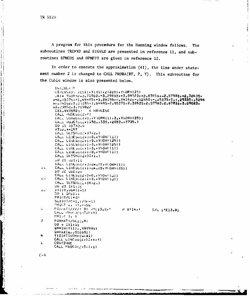
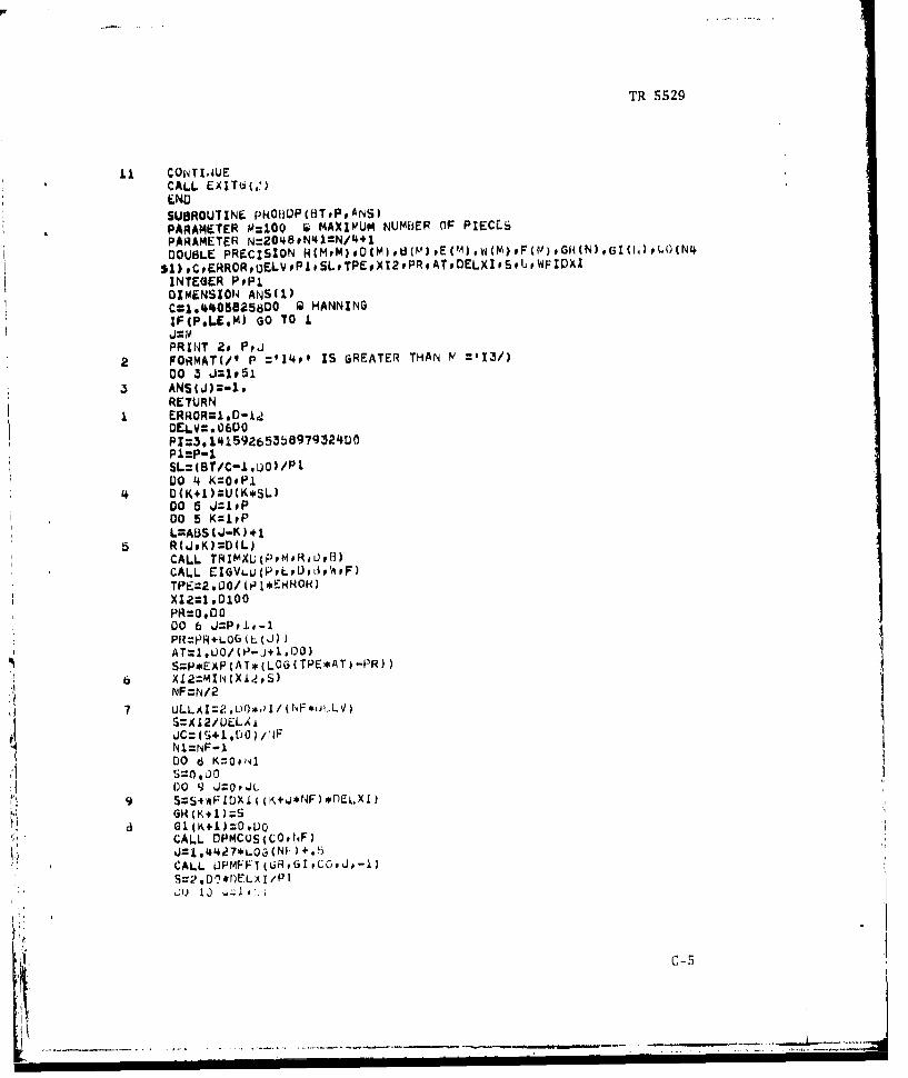
A program for this procedure for the Hanning window follows. Thesubroutines TRIMXD and EIGVLD are presented in reference 11, and sub-

routines DPMCOS and DPMFFT are given in reference 12.

In order to execute the approximation (41), the line under state-ment number 2 is changed to CALL PROBA(BT, P, Y). This subroutine for

the Cubic window is also presented below.

*,.il~ujt.'ý-ib1. 644 .o2 *o5375,2. 32635 .2.57983,2.878l6 .3.09023.

C=1 .'440582ý i (i HIsANIING 3YFO(2)

'I ~~~~CALL .hD.,a,'

CALL I)tjjiEuL~.jtO. *YN.OH(±) o275

CALiý!LTLSHJ$(.-'p.31 #2-.YOw(~

CALL LlfJLSG (4'p IPi. PYN0HP (2))CALL LIIIL au (t. 10S. #YNOIt(1))CALL ~~M~L3,.UU 21 Q=z1,jCALL L Ir iL.~' k,' j 5 P yI i HR M( I1

A. CALL LIHEti (I PX.1.J*.ýB.5p YHOw.(Pb))

CALL LINE ~(ZPO#.t.Yr1Om1i(J))r~CALL LLNES (Z.I#i.PYtJOHN-CJ))

CALL SLTSI'iI , P.'.0 P~.)

U3O 23 1=1,5i

PH~fT , 11,PSL

L0 .4 1:1.51

'4 Y(Z)=T1r4ONN.(wt1)CALL LIN[~b6(Z0ý10XP. f

I coNrIVtJECALL. PAGEG(,0,~i11)

C- 4

TR 5529

I1 COiqTI.4UECALL E)1T6(,')

SUBROUTINE fPNOI3QP(tHTtPpANS)PARAMETER M:100 Ii MAXIWUM NUMbSEP OF PIECLS,PARAMETER N=2O48PN*41=N/~4+1DOUBLE PRECISION NCMM),0(M~,pCMvE(M1),w(M),F(fO),GH(N),GI(h.),LU(N4

SI) eCERRORPUELVPP1SLeTPEeXI2,PRoATPDELXIeSPUWFIDXIINTEGER PPPDIMENSION ANS(1)CXi1944058258D0 Q HANNINGIF(PsL.1.M) GO TO I

PRI14T 2o Ppi2 FORMATW/ P zt14e' IS GREATER THAN =#3/

00 3 Ja1,513 ANS(J)Z-I.

RETURNL ERROR=1.D-i.2

DELV=.06C)OPlz3. IQ159265358979324uOP1=P-1SL=(BT/C-1,Uo)/PIDO 4 K=0,P1

4 D(K+1)=U(K*SL)00 5 ~Jz1,PDO 5 KZPP

5 RC(J#K)=D(LICALL TRlXMU(FpPMoRsLJpf.3)CALL EZGVLWL(PLPDLiArF)TPE~22v00/ tP I*ENHOK)X12=1 .0100PR:0,D000 6 jpl-PR=PR+LOG.'L(J))

S=P*EXP(AT*(LOG(TPE*AThfPR))A

NF :N/

7 ULLAI=2,Lt)*dI/(NF*u)LLV

N1=NF-1

00 '9 Jzc,.Jc9 5=S4*FlrDX4fl(K+,.j*NF)*flEL.X1)

GH(K+I )=Sa GL(K+I)=O.IJ0

CALL OPMC0S(C0#hF)J= 442~7WL0,3(NfI) +. 5CALL UPMFFT 1ýR,GI ,coo.Jp-1)S=2.0'*r0ELXI/Pt

c-5

TR 5529

10 AI 14 S I D0 5H(IF(iiF.Er1~.ii) RETURNUU It 4ZIP14605

11 PRINT 120 AN(JPN(+~~i(+PptSJ3piSJ4(I PRINT 12o ANS(51)12 FORNIAT(/5E20.8)

NF:N4GO TO IFUNCTIUN Ui(T) H~IANNINGDO0UOLI PRECZSIVN ToSlIFTG,~o GO TO ISlz2o00*PI .rRE TUR14U=0100RETUR1NFUNCTION WFZUXI(X)

DIUEPLI1,XXO#APlp~pr,,pý

lFOXIF CSQ*(X* GOR)* TO i.U IfO:~ (?P

vWFIUXI:-EL/(¶S*XRETURNI

CI.820096 UIC

SL:-(PTcj.)v/PIDO1

TE0P1. K8j*pjl

id AL=T FLATEI/)*(KSL**CQAPKL*AP/E*Ii

PRINT 1O1(XTOApX

UG 5 K:I~,II3

RETUREN 6

UNCLASSIFIED R52

5 GDZGD+LOG (c)DO 3 =5 bV:,06*(K-1)IF(VvGT,0*) GO TO 6:1 ANS(K):0.60 TO 3

6 BVZU*VANS(K):EXPCB.LOG(B3V)-BV.FUIL(DBLEIB,1.) BV)-0Q)

3 CONTINUERETURN

2 PRINT 4, 84 FORMAT(# PROBLEM AT 8 = E15*8)

RETURNFUNCTION FILL(AeXU)DOUB~LE PRECISION SDPTDPADtXD-PA

ADZA-J, 0000 1 K=XvI000TD:TD*XU/(AO+K)

I ZF(ABS(TU).LE4.oD-6*A8Sl(508 W O 102PRINT 3,

*3 FORMAT(/, 1000 TERMSV/)a F1IL:=LOG(50)

RETURNFUNCTION W(JT) Q CUBICZF(T.GE,1.) Go To I

IF(T.GE.O,75) RETURNU=U-8192@/151.*( .75-T)**7xr(T.GE,O.5) RETURNU=V+28b72o/15ls*( .5-T)**7IF(TGE.Oo25) RETURNU=U-57344./j51o*(*25-T)**7RETURN

1 U:D.RETURNEND

C-7/C- 8

UNCLASSIFIED vrsBlk

TR 5529

REFERENCES

1. A. I. Nuttall, Spectral .... Estinmat.io FaEx~i~.r.rTT!j form Process in.f.Win d__ood Dat.a, NUSC Technical

Report 4169, 13 October 1971.

2. A. I1. Nuttall, Estimation of Cross-Spectra via Overlapned FastFourier Transform Processing, NUSC Technical Report 4169-S,11 July 1975. (Also NUSC Technical Memorandum TC-83-72, 18 April1972.)

3. A. H. Nuttall, Numerical Evaluation of Cumulative ProbabilityDistribution Functions Directly from Characteristic Functions,'USL Report 1032, 11 August 1969. (Also Proc. IEEE, vol. 57, no, 11,Nov. 1969, pp. 2071-2072.)

4. A. II. Nuttall, Alternate Forms and Computational Considerations furNumerical Evaluation of Cumulative Probability DistributionsFirrectly from Characteristic Functions, NUSC Report NL-3012,12 August 1970. (Also Proc. IEEE, vol. 58, no. 11, Nov. 1970,pp. 1872-1873.)

5. M. M. Siddiqui, Approximations to the Distribution of QuadraticForms," The Annals of Mathematical Statistics, vol. 36, 1965,

pp. 677-682.-

6. Handbook of Mathematical Functions, U. S. Dept. of Comm., NationalBureau of Standards, Applied Mathematics Series, no. 55, U. S.Government Printing Office, Washington, D.C., June 1964.

7. A. H. Nuttall, Spectral Estimation of a Univariate Process withBad Data Points, via Maximum Entropy and Linear Pred€-ttveTechniques, NUSC Technical Report 5303, 26 March 1976.

8& . H. Nuttall, Multivariate Linear Predictive Spectral Analysis,E mip].oyipg Weigh~ted Forward and Backward Averag.ing: A General izat ion

of Burk's Algorjthm, NUSC Technical Report 5501, 13 October 1976.(Also) program Is in NUSC Technical Document 5419, 19 May 1976.)

9, A. H. Nuttall and P. G. Cable, Operating Characteristics forMaximum Likelihood Detection of 9 in Gd6s-anNoise-- fVnkno-- Leveli; Part I, Coherent Si&nals of_ Unknown Levey NUSC

- I Technical Report 4243, 27 March 1972.

"R-1

S. ...... ---.-..---.. _..'

TR 5529

REFERENCIHS (Cont 'd)

10. G, L. Turin, "The Characteristic Function of [iermitian QuadraticForms in Complex Normal Variables," Biometrika, vol. 47, nos. Iand 2, 1960, pp. 199-201,

11. M. J. Goldstein and N. Broc:kman, "On Several Double PrecisionSubroutines for Computing Oh, I3igenvalues and/or Higenvectors ofHlermitian Matrices," NUSC Thehnical Memorandum 2070-253-70,10 July 1970.

12. 1. F. Fcorrie, "Double Precisioon Version of Markel's FFT Algorithm,"NUSC Technical Memorandum TiD 113-15-73, 11 June 1973.

R-2

TR 5529

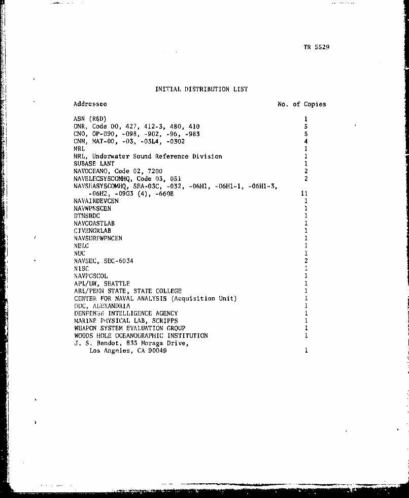
INITIAL DISTRIBUTION LIST

Addressee No. of Copies

ASN (R&D) 1ONR, Code 00, 427, 412-3, 480, 410 5CNO, OP-090, -098, -902, -96, -983 5CNM, MAT-00, -03, -03L4, -0302 4NRL 1NRL, Underwater Sound Reference Division 1SUBASE LANT 1NAVOCFANO, Code 02, 7200 2NAVELECSYSCOMHQ, Code 03, 051 2NAVSEASYSCOMHQ, SEA-03C, -032, -06H1, -06H1-1, -06H1-3,

-06H2, -09G3 (4), -660E 11NAVAI RDEVCEN 1NAVWPNSCEN 1DTNSRDC 1NAVCOASTLAB 1CIVPNGRLAB INAVSURFWPNCEN 1NrLC 1NUC INAVSEC, SEC-6034 2NISC INAVPGSCOL 1APL/UW, SEATTLE 1

J ARL/PEffN STATE, STATE COLLEGE 1CENTER FOR NAVAL ANALYSIS (Acquisition Unit) 1l)DC, ALXXANDRIA 1DENFEN'Ii INTELLIGENCE AGENCY IMARINE PHYSICAL LAB, SCRIPPS IWEAPON SYSTEM EVALUATION GROUP 1WOODS HOLE OCEANOGRAPHIC INSTITUTION 1J. S. Bendot, 833 Moraga Drive,

Los Angnles, CA 90049 1

S. . . .. .. . . .. . . . . . . . . . ..I. • • . • .. . . .. .