routing & scheduling: part 1. transport service selection depends on variety of service...
TRANSCRIPT

Routing & Scheduling:Routing & Scheduling:Part 1Part 1
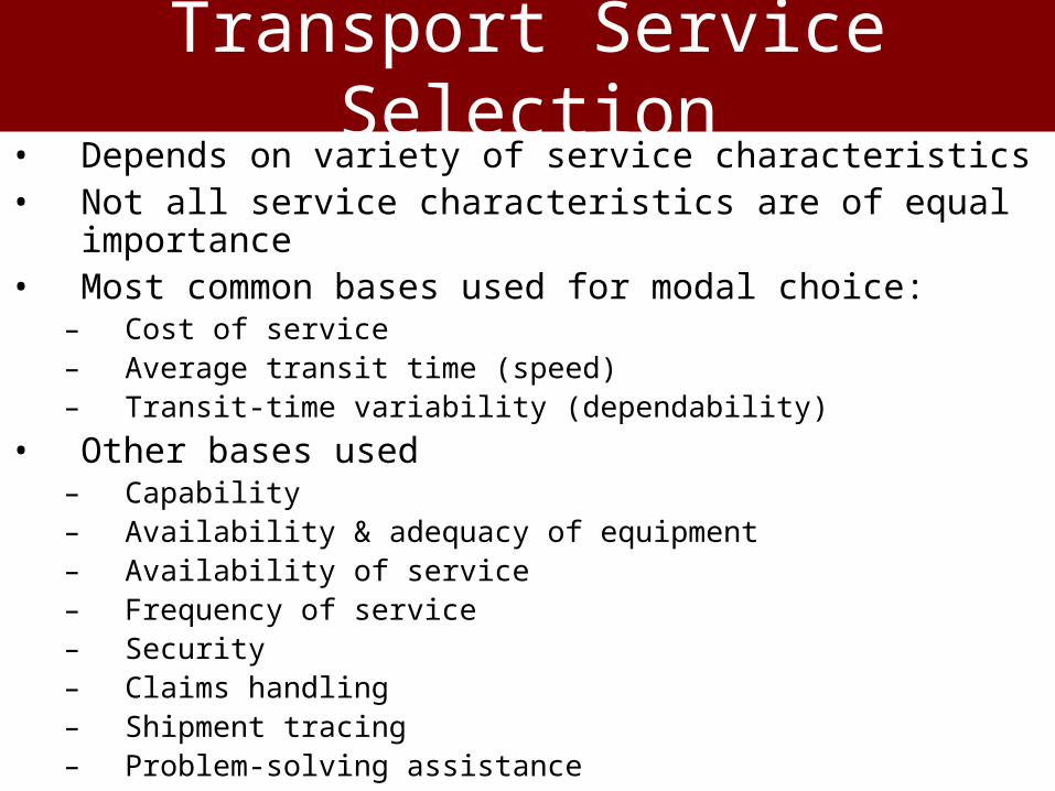
Transport Service Selection• Depends on variety of service characteristics• Not all service characteristics are of equal importance• Most common bases used for modal choice:
– Cost of service– Average transit time (speed)– Transit-time variability (dependability)
• Other bases used– Capability– Availability & adequacy of equipment– Availability of service– Frequency of service– Security– Claims handling– Shipment tracing– Problem-solving assistance

Basic Cost Trade-Offs• When alternative modes are available, the one
chosen should be the one that offers the lowest total cost consistent with customer service goals.
• Often, cost trade-offs must be used.
• Speed & dependability affect both the seller’s & buyer’s inventory level, as well as the inventory that is in transit.
• Slower, less reliable modes require more inventory in the distribution channel

Example• A Birmingham luggage company maintains a finished-
goods inventory at its plant• Currently, rail is used to ship between Birmingham and
the firm’s West Coast warehouse• Average transit time is T = 21 days• 100,000 units are kept at each stocking point with the
luggage having an average value of C = $30 per unit• Inventory carrying costs are I = 30 percent per year• There are D = 700,000 units sold per year out of the West
Coast warehouse• Average inventory levels can be reduced by 1 percent for
each day of transit time that is eliminated.
Example
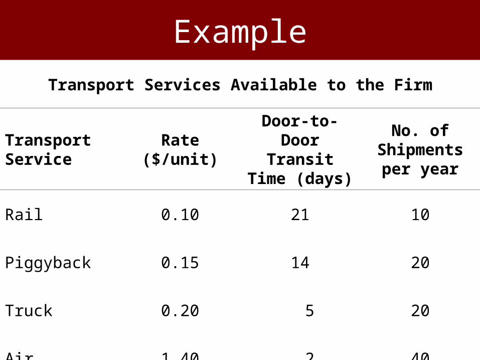
Transport Services Available to the Firm
Transport Service
Rate ($/unit)Door-to-Door Transit Time
(days)
No. of Shipments per
year
Rail 0.10 21 10
Piggyback 0.15 14 20
Truck 0.20 5 20
Air 1.40 2 40

Example• Different modes affect the time inventory is in transit• Annual demand (D) will be in transit by the fraction of the
year represented by T/365 days, where T is the average transit time
• Annual cost of carrying this in-transit inventory is ICDT/365
• Average inventory at both ends of the channel can be approximated as Q/2, where Q is the shipment size
• Holding cost per unit is I x C– Note that C must reflect where the inventory is in the channel– Value of C at the plant is the price ($30 per unit)– Value of C at the WC warehouse is C + transportation rate
• Total annual transportation cost is R x D

Example
Cost TypeMethod of
ComputationRail
Transportation R x D (.1)(700,000) = 70,000
In-transit Inventory ICDT/365[(.3)(30)(700,000)(21)]/365 =
363,465
Plant Inventory ICQ/2 [(.3)(30)(100,000)] = 900,000
Warehouse Inventory IC”Q/2 [(.3)(30.1)(100,000)] = 903,000
Total for Rail $2,235,465
Example
Cost TypeMethod of
ComputationPiggyback
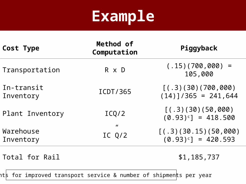
Transportation R x D (.15)(700,000) = 105,000
In-transit Inventory ICDT/365[(.3)(30)(700,000)(14)]/365 =
241,644
Plant Inventory ICQ/2[(.3)(30)(50,000)(0.93)c] =
418.500
Warehouse Inventory IC”Q/2[(.3)(30.15)(50,000)(0.93)c] =
420.593
Total for Rail $1,185,737
C = accounts for improved transport service & number of shipments per year

Example
Cost TypeMethod of
ComputationTruck
Transportation R x D (.2)(700,000) = 140,000
In-transit Inventory ICDT/365[(.3)(30)(700,000)(5)]/365 =
86,301
Plant Inventory ICQ/2[(.3)(30)(50,000)(0.84)c] =
378,000
Warehouse Inventory IC”Q/2[(.3)(30.2)(50,000)(0.84)c] =
380,520
Total for Rail $984,821
C = accounts for improved transport service & number of shipments per year

Example
Cost TypeMethod of
ComputationAir
Transportation R x D (1.4)(700,000) = 980,000
In-transit Inventory ICDT/365[(.3)(30)(700,000)(2)]/365 =
34,521
Plant Inventory ICQ/2[(.3)(30)(25,000)(0.80)c] =
378,000
Warehouse Inventory IC”Q/2[(.3)(30.4)(25,000)(0.80)c] =
190,755
Total for Rail $1,387,526
C = accounts for improved transport service & number of shipments per year

Example
Modal Choice
Cost TypeMethod of
ComputationRail Piggyback Truck Air
Transportation R x D 70,000 105,000 140,000 980,000
In-transit Inventory
ICDT/365 363,465 241,644 86,301 34,521
Plant Inventory ICQ/2 900,000 418,500 378,000 182,250
Warehouse Inventory
IC”Q/2 903,000 420,593 380,520 190,755
Totals $2,235465 $1,185,737 $984,821 $1,387,526

Factors Other Than Transportation Cost that Affect Modal Choices
• Effective buyer/seller cooperation is encouraged if a reasonable knowledge of the other party’s costs is available
• If there are competing suppliers, buyer & supplier should act rationally to gain optimum cost-transport service trade-offs
• Offering higher-quality transportation services than the competition may allow the seller to charge a higher price for the product
• Elements in the mix change frequently– Transport rate fees, product mix changes, inventory cost
changes, & transport service retaliation by competitors• If buyer makes the transport choice, seller’s inventories
are impacted as well, which may impact price charged for the product
Vehicle Routing & Scheduling
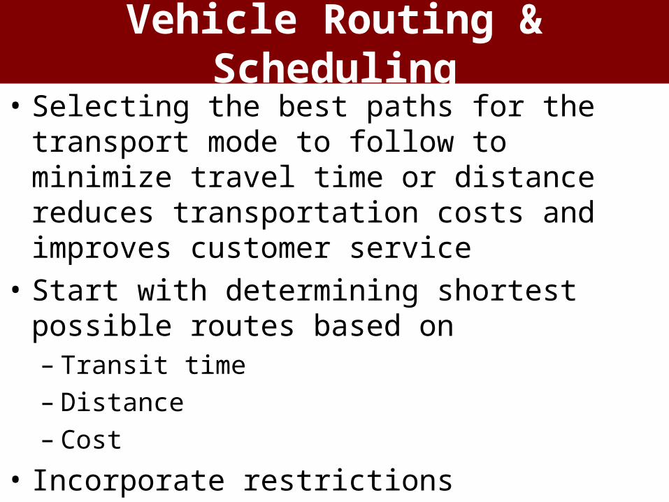
• Selecting the best paths for the transport mode to follow to minimize travel time or distance reduces transportation costs and improves customer service
• Start with determining shortest possible routes based on– Transit time– Distance– Cost
• Incorporate restrictions

Restrictions on Vehicle Routing & Scheduling
• Each stop on the route may have volume to be picked up as well as delivered
• Multiple vehicles may be used using different capacity limits to both weight and cube
• Maximum total driving time allowed before a rest period must be taken is 8 hours
• Stops may permit pickups/deliveries only at certain times of day (time windows)
• Pickups may be permitted on a route only after deliveries are made
• Drivers may be allowed to take short rests or lunch breaks at certain times of the day.
8 Principles for Good Routing & Scheduling
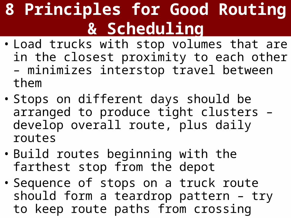
• Load trucks with stop volumes that are in the closest proximity to each other – minimizes interstop travel between them
• Stops on different days should be arranged to produce tight clusters – develop overall route, plus daily routes
• Build routes beginning with the farthest stop from the depot
• Sequence of stops on a truck route should form a teardrop pattern – try to keep route paths from crossing

8 Principles for Good Routing & Scheduling
• The most efficient routes are built using the largest vehicles available – allocate largest vehicles first, then smaller
• Pickups should be mixed into delivery routes rather than assigned to the end of routes
• A stop that is greatly removed from the other stops in a route cluster is a good candidate for an alternative means of delivery
• Narrow stop time window restrictions should be avoided – see if you can renegotiate the time window restrictions
Routing & Scheduling:Routing & Scheduling:Part 2Part 2
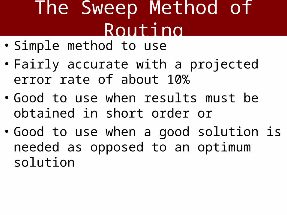
The Sweep Method of Routing• Simple method to use
• Fairly accurate with a projected error rate of about 10%
• Good to use when results must be obtained in short order or
• Good to use when a good solution is needed as opposed to an optimum solution
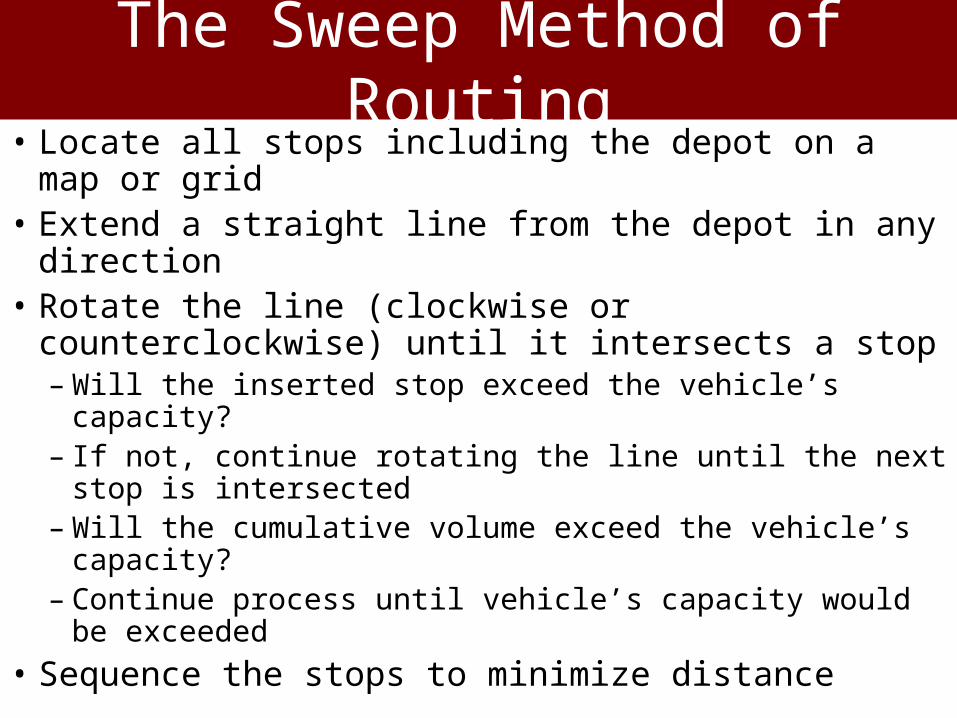
The Sweep Method of Routing• Locate all stops including the depot on a map or grid• Extend a straight line from the depot in any direction• Rotate the line (clockwise or counterclockwise) until
it intersects a stop– Will the inserted stop exceed the vehicle’s capacity?– If not, continue rotating the line until the next stop is
intersected– Will the cumulative volume exceed the vehicle’s capacity?– Continue process until vehicle’s capacity would be
exceeded
• Sequence the stops to minimize distance

Sweep Method Example• Gofast Trucking uses vans to pickup merchandise
from outlying customers
• Merchandise is returned to a depot where it is consolidated into large loads for intercity transport
• Firm’s vans can haul 10,000 units
• Completing a route typically takes a full day
• Firm wants to know– How many routes (trucks) are needed– Which stops should be on the routes– And sequence of stops for each truck

Sweep Method Example
A
2000
B
3000
C
2000
D
3000
E
1000
F
3000
G
2000
H
4000
I
1000
J
2000
K
2000
L
2000
Depot
Pickup Stop Data: quantities shown in units

Sweep Method Example
A
2000
B
3000
C
2000
D
3000
E
1000
F
3000
G
2000
H
4000
I
1000
J
2000
K
2000
L
2000
Depot
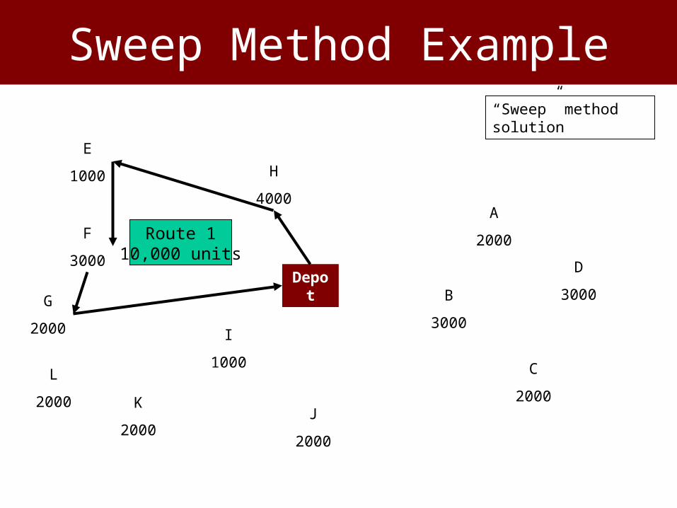
“Sweep” method solution
Sweep Method Example
A
2000
B
3000
C
2000
D
3000
E
1000
F
3000
G
2000
H
4000
I
1000
J
2000
K
2000
L
2000
Depot
“Sweep” method solution
Route 110,000 units

Sweep Method Example
A
2000
B
3000
C
2000
D
3000
E
1000
F
3000
G
2000
H
4000
I
1000
J
2000
K
2000
L
2000
Depot
“Sweep” method solution
Route 110,000 units
Route 29,000 units
Route 38,000 units
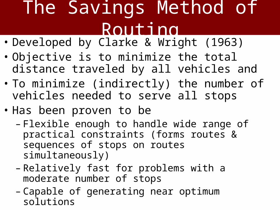
The Savings Method of Routing• Developed by Clarke & Wright (1963)• Objective is to minimize the total distance traveled
by all vehicles and• To minimize (indirectly) the number of vehicles
needed to serve all stops• Has been proven to be
– Flexible enough to handle wide range of practical constraints (forms routes & sequences of stops on routes simultaneously)
– Relatively fast for problems with a moderate number of stops
– Capable of generating near optimum solutions

The Savings Method of Routing• Begin with a dummy vehicle serving each stop and
returning to the depot.– Gives the maximum distance to be experienced in the routing
problem
• Two stops are then combined together on the same route– Eliminates one vehicle and travel distance is reduced
• To determine which stops to combine on a route, the distance saved is calculated before and after each combination– This calculation is repeated for all stop pairs
– The stop pair with the largest savings value is selected to be combined

The Savings Method of Routing
Depot (0)
Stop A
Stop B
d0,A
d0,B
dA,0
dB,0
Initial routing – Route distance= d0,A + dA,0 + d0,B + dB,0
The Savings Method of Routing
Depot (0)
Stop A
Stop B
d0,A
dA,B
dB,0
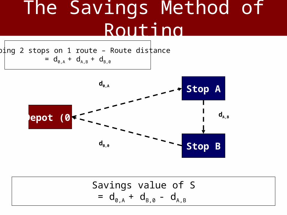
Combing 2 stops on 1 route – Route distance= d0,A + dA,B + dB,0
Savings value of S= d0,A + dB,0 - dA,B

The Savings Method of Routing
Jacksonville (0)
Atlanta (A)
Birmingham (B)
d0,A = 100
d0,B = 85
dA,0 = 100
dB,0 = 85
Initial routing – Route distance= d0,A + dA,0 + d0,B + dB,0
Initial routing – Route distance= d0,A(100) + dA,0(100) + d0,B(85) + dB,0(85) = 370 miles total

The Savings Method of Routing
Jacksonville (0)
Atlanta (A)
Birmingham (B)
dA,B = 145
Combining 2 stops on 1 route – Route distance= d0,A(100) + dA,B(145) + dB,0(85) = 330 total miles
Savings value of S = d0,A(100) + dB,0(85) - dA,B(145) = 40 miles saved
d0,A = 100
dB,0 = 85

The Savings Method of Routing• If a third stop (C) is to be inserted between stops A
and B, where A and B are on the same route, the savings value is expressed as
• S = d0,C + dC,0 + dA,B - dA,C - dC,B
• If stop C were inserted after stop B, the savings value is expressed as
• S = dB,0 - dB,C + d0,C
• If stop C were inserted before stop A, the savings value is expressed as
• S = dC,0 - dC,A + d0,A

The Savings Method of Routing
Depot (0)
Stop A
Stop B
d0,A
d0,B
dA,0
dB,0
Initial routing – Route distance= d0,A + dA,0 + d0,B + dB,0 + d0,C + dC,0
Stop Cd0,C
dC,0

The Savings Method of Routing
Depot (0)
Stop A
Stop B
d0,A
dA,B
dC,0
Combining 3 stops on 1 route – Route distance (additional stop added after 1st 2 stops)= d0,A + dA,B + dB,C + dC,0
Savings value of S = d0,C + dC,0 + dA,B - dA,C - dC,B
Stop C
dB,C

The Savings Method of Routing
Jacksonville (0)
Atlanta (A)
Birmingham (B)
d0,A = 100
d0,B = 85
dA,0 = 100
dB,0 = 85
Initial routing – Route distance = d0,A(100) + dA,0 (100) + d0,B(85) + dB,0 (85) + d0,C (25) + dC,0 (25) = 420 total miles
Gadsden (C)
d0,C = 25
dC,0 = 25

The Savings Method of Routing
Depot (0)
Atlanta (A)
Birmingham (B)
d0,A = 100
dA,B = 145
dC,0 = 25
Combining 3 stops on 1 route – Route distance (additional stop added after 1st 2 stops)= d0,A(100) + dA,B(145) + dB,C(65) + dC,0(25) = 335 miles
Savings value of S = dB,0 (85) - dB,C(65) + d0,C(25) = 45 miles savedEarlier O to A to B to O route (330 miles) plus 0 to C to 0 route (50 miles) = 380 miles
Gadsden (C)
dB,C = 65
The Savings Method of Routing
Depot (0)
Atlanta (A)
Gadsden (C)
d0,A = 100
dA,C = 125
dB,0 = 85
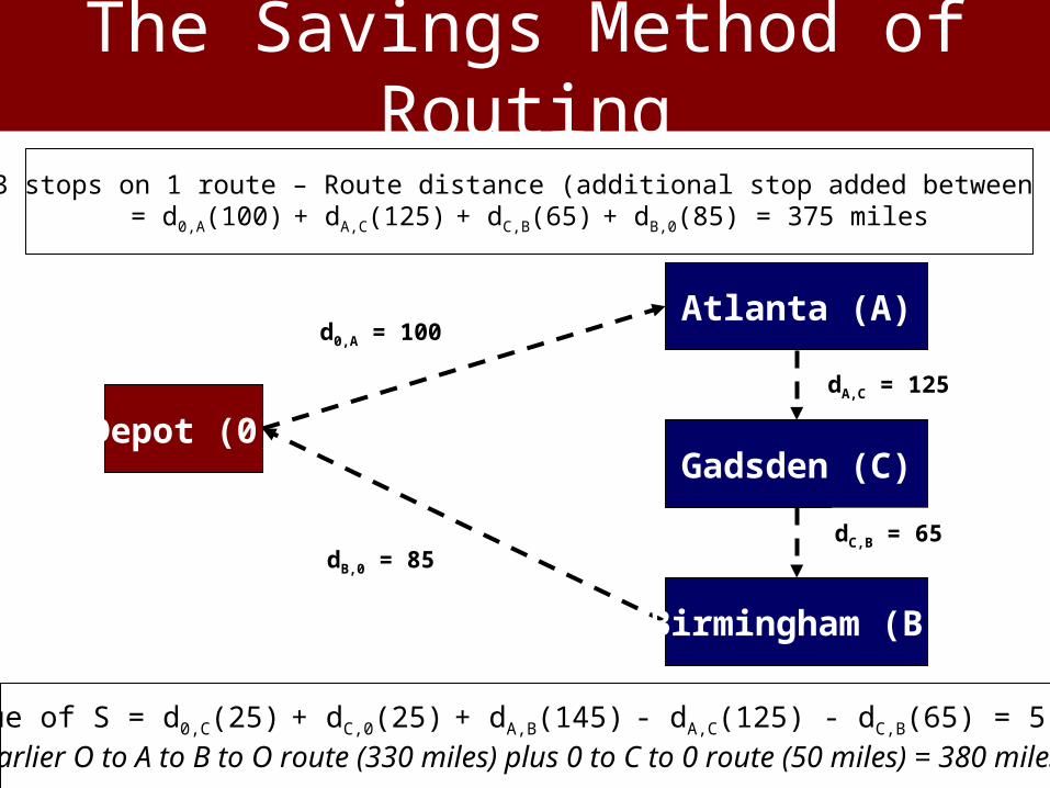
Combining 3 stops on 1 route – Route distance (additional stop added between 1st 2 stops)= d0,A(100) + dA,C(125) + dC,B(65) + dB,0(85) = 375 miles
Savings value of S = d0,C(25) + dC,0(25) + dA,B(145) - dA,C(125) - dC,B(65) = 5 miles savedEarlier O to A to B to O route (330 miles) plus 0 to C to 0 route (50 miles) = 380 miles
Birmingham (B)
dC,B = 65

The Savings Method of Routing
Depot (0)
Gadsden (C)
Atlanta (A)
d0,C = 25
dC,A = 125
dB,0 = 85
Combining 3 stops on 1 route – Route distance (additional stop added before 1st 2 stops)= d0,C(25) + dC,A(125) + dA,B(145) + dB,0(85) = 380 miles
Savings value of S = dC,0(25) - dC,A(125) + d0,A(100) = 0 miles savedEarlier O to A to B to O route (330 miles) plus 0 to C to 0 route (50 miles) = 380 miles
Birmingham (B)
dA,B = 145

The Savings Method of Routing
When 3rd Stop Added
Routes Added
Routes Eliminated
Miles Saved
After 1st 2 B > C; C > 0 B > 0 45
Between 1st 2 A > C; C > B0 > C; C > 0;
A > B5
Before 1st 2 C > A 0 > A; C > 0 0