Performance Characteristics of In-Service Bridges for Enhancing Load Ratings: Leveraging Refined Analysis Methods

http://www.virginiadot.org/vtrc/main/online_reports/pdf/21-r20.pdf

DEVIN K. HARRIS, Ph.D. Associate Professor Department of Engineering Systems and Environment University of Virginia OSMAN OZBULUT, Ph.D. Associate Professor Department of Engineering Systems and Environment University of Virginia ABDOU K. NDONG Graduate Research Assistant Department of Engineering Systems and Environment University of Virginia MUHAMMAD SHERIF Assistant Professor Department of Civil, Construction and Environmental Engineering University of Alabama at Birmingham

Final Report VTRC 21-R20

Standard Title Page - Report on Federally Funded Project

1. Report No.: 2. Government Accession No.: 3. Recipient’s Catalog No.:

FHWA/VTRC 21-R20

4. Title and Subtitle: 5. Report Date:

Performance Characteristics of In-Service Bridges for Enhancing Load Ratings:

Leveraging Refined Analysis Methods

March 2021

6. Performing Organization Code:

7. Author(s):

Devin K. Harris, Ph.D., Osman Ozbulut, Ph.D., Abdou K. Ndong, and Muhammad

Sherif

8. Performing Organization Report No.:

VTRC 21-R20

9. Performing Organization and Address:

Virginia Transportation Research Council

530 Edgemont Road

Charlottesville, VA 22903

10. Work Unit No. (TRAIS):

11. Contract or Grant No.:

114318

12. Sponsoring Agencies’ Name and Address: 13. Type of Report and Period Covered:

Virginia Department of Transportation

1401 E. Broad Street

Richmond, VA 23219

Federal Highway Administration

400 North 8th Street, Room 750

Richmond, VA 23219-4825

Final Contract

14. Sponsoring Agency Code:

15. Supplementary Notes:

This is an SPR-B report.

16. Abstract:

Bridge load rating assesses the safe live load carrying capacity of an existing or newly designed structure. In addition to

load rating with previously defined standard load rating vehicles, the Federal Highway Administration issued additional guidance

to states related to rating requirements for all the bridges with respect to specialized hauling vehicles and emergency vehicles that

must be met by the end of 2022. It is recognized that the load effects (bending moment and shear) produced by these vehicle

types on certain bridge types and spans might be greater than those caused by the previous rating vehicles. Therefore, a number

of bridges within VDOT’s inventory may require posting when rated with these specialized vehicles.

The goal of this study was to assess the likelihood of an increase in load rating factors through refined analysis methods

for the bridge classes potentially vulnerable to load ratings under consideration of the new federal regulations and when using

conventional, simplified equations for load distribution factors. In particular, the study focused on the evaluation of live load

distribution factors for girder bridges and effective widths for distributing live loads in slab bridges through refined analysis.

Three bridge classes (simple span steel girder bridges, reinforced concrete T-beam bridges, and concrete slab bridges) were

selected for this refined analysis. Girder bridges were modeled using the plate-with-an-eccentric-beam analysis approach, while

plate elements were used to model slab bridges within the LARSA 4D software package. The selected modeling approaches were

validated through the simulation of the bridge structures with available field-testing results from the literature. A total of 71 in-

service bridges belonging to the three selected bridge classes were then modeled and analyzed to compute the load distribution

factors for girder bridges or effective widths for slab bridges, and the results were compared with those obtained from the code-

specified equations. Using the data obtained from these numerical simulations, a series of multi-parameter linear regression

models were developed to predict the percent change in distribution factor and effective width, respectively, for girder and slab

bridges with different geometrical characteristics if a refined method analysis is implemented. The regression models were

limited to four parameters such that the results from regression models could be presented in table format.

The developed tables should be used as screening tools to provide guidance on the use of refined methods of analysis to

improve the load ratings of bridges vulnerable to posting from previously existing load rating classifications as well as the

recently introduced vehicles. Should VDOT use refined methods of analysis, there is good potential that the agency can avoid

posting a substantial portion of its inventory, saving resources for more critical needs while safely keeping Virginia’s bridges

open for commerce and the traveling public.

17 Key Words: 18. Distribution Statement:

load rating, live load distribution factors, effective widths,

refined analysis

No restrictions. This document is available to the public

through NTIS, Springfield, VA 22161.

19. Security Classif. (of this report): 20. Security Classif. (of this page): 21. No. of Pages: 22. Price:

Unclassified Unclassified 52

Form DOT F 1700.7 (8-72) Reproduction of completed page authorized

FINAL REPORT

PERFORMANCE CHARACTERISTICS OF IN-SERVICE BRIDGES

FOR ENHANCING LOAD RATINGS: LEVERAGING REFINED ANALYSIS

METHODS

Devin K. Harris, Ph.D.

Associate Professor

Department of Engineering Systems and Environment

University of Virginia

Osman Ozbulut, Ph.D.

Associate Professor

Department of Engineering Systems and Environment

University of Virginia

Abdou K. Ndong

Graduate Research Assistant

Department of Engineering Systems and Environment

University of Virginia

Muhammad Sherif

Assistant Professor

Department of Civil, Construction and Environmental Engineering

University of Alabama at Birmingham

VTRC Project Manager

Bernard L. Kassner, Ph.D., P.E., Virginia Transportation Research Council

In Cooperation with the U.S. Department of Transportation

Federal Highway Administration

Virginia Transportation Research Council

(A partnership of the Virginia Department of Transportation

and the University of Virginia since 1948)

Charlottesville, Virginia

March 2021

VTRC 21-R20

ii

DISCLAIMER

The project that is the subject of this report was done under contract for the Virginia

Department of Transportation, Virginia Transportation Research Council. The contents of this

report reflect the views of the author(s), who is responsible for the facts and the accuracy of the

data presented herein. The contents do not necessarily reflect the official views or policies of the

Virginia Department of Transportation, the Commonwealth Transportation Board, or the Federal

Highway Administration. This report does not constitute a standard, specification, or regulation.

Any inclusion of manufacturer names, trade names, or trademarks is for identification purposes

only and is not to be considered an endorsement.

Each contract report is peer reviewed and accepted for publication by staff of Virginia

Transportation Research Council with expertise in related technical areas. Final editing and

proofreading of the report are performed by the contractor.

Copyright 2021 by the Commonwealth of Virginia.

All rights reserved.

iii

ABSTRACT

Bridge load rating assesses the safe live load carrying capacity of an existing or newly

designed structure. In addition to load rating with previously defined standard load rating

vehicles, the Federal Highway Administration issued additional guidance to states related to

rating requirements for all the bridges with respect to specialized hauling vehicles and

emergency vehicles that must be met by the end of 2022. It is recognized that the load effects

(bending moment and shear) produced by these vehicle types on certain bridge types and spans

might be greater than those caused by the previous rating vehicles. Therefore, a number of

bridges within VDOT’s inventory may require posting when rated with these specialized

vehicles.

The goal of this study was to assess the likelihood of an increase in load rating factors

through refined analysis methods for the bridge classes potentially vulnerable to load ratings

under consideration of the new federal regulations and when using conventional, simplified

equations for load distribution factors. In particular, the study focused on the evaluation of live

load distribution factors for girder bridges and effective widths for distributing live loads in slab

bridges through refined analysis. Three bridge classes (simple span steel girder bridges,

reinforced concrete T-beam bridges, and concrete slab bridges) were selected for this refined

analysis. Girder bridges were modeled using the plate-with-an-eccentric-beam analysis approach,

while plate elements were used to model slab bridges within the LARSA 4D software package.

The selected modeling approaches were validated through the simulation of the bridge structures

with available field-testing results from the literature. A total of 71 in-service bridges belonging

to the three selected bridge classes were then modeled and analyzed to compute the load

distribution factors for girder bridges or effective widths for slab bridges, and the results were

compared with those obtained from the code-specified equations. Using the data obtained from

these numerical simulations, a series of multi-parameter linear regression models were developed

to predict the percent change in distribution factor and effective width, respectively, for girder

and slab bridges with different geometrical characteristics if a refined method analysis is

implemented. The regression models were limited to four parameters such that the results from

regression models could be presented in table format.

The developed tables should be used as screening tools to provide guidance on the use of

refined methods of analysis to improve the load ratings of bridges vulnerable to posting from

previously existing load rating classifications as well as the recently introduced vehicles. Should

VDOT use refined methods of analysis, there is good potential that the agency can avoid posting

a substantial portion of its inventory, saving resources for more critical needs while safely

keeping Virginia’s bridges open for commerce and the traveling public.

1

FINAL REPORT

PERFORMANCE CHARACTERISTICS OF IN-SERVICE BRIDGES

FOR ENHANCING LOAD RATINGS: LEVERAGING REFINED ANALYSIS

METHODS

Devin K. Harris, Ph.D.

Associate Professor

Department of Engineering Systems and Environment

University of Virginia

Osman Ozbulut, Ph.D.

Associate Professor

Department of Engineering Systems and Environment

University of Virginia

Abdou K. Ndong

Graduate Research Assistant

Department of Engineering Systems and Environment

University of Virginia

Muhammad Sherif

Assistant Professor

Department of Civil, Construction and Environmental Engineering

University of Alabama at Birmingham

INTRODUCTION

According to the 2019 State of the Structures and Bridges Report by the Virginia

Department of Transportation’s (VDOT) Structure and Bridge Division (VDOT 2019), there are

21,173 bridges and culverts in the Commonwealth, of which, VDOT maintains 19,598. VDOT

inspects more than 10,000 of these structures annually, including bridges that are less than 20 ft

long and culverts that have openings that are 36 ft2 or greater. These inspections ensure the safe

and secure operation of transportation infrastructure in Virginia, as required by the National

Bridge Inspection Standards (NBIS), but also provide a measure of condition state and its

evolution over time. More importantly, inspection results are used as inputs to inform capacity

determinations and ultimately contribute to the determination of a bridge’s load rating, or safe

live load carrying capacity. Thus, load ratings are critical in prioritizing maintenance operations

and allocation of resources. Equally important, these ratings have a direct impact on the

movement of goods and services within the Commonwealth, as postings resulting from low load

ratings require vehicles exceeding these postings to find alternative paths.

In 2013, the Federal Highway Administration (FHWA) mandated state departments of

transportation to rate all bridges within the state inventory for a class of vehicles called

specialized hauling vehicles (SHVs) by the end of 2017 for Group 1 bridges (i.e., those bridges

2

whose shortest span is not greater 200 ft and load rating or rating factor is below a certain value)

and by the end of 2022 for Group 2 bridges (i.e., all bridges that are not in Group 1), unless state

laws preclude SHV use (FHWA 2013). In addition, the 2015 Fixing America’s Surface

Transportation Act (FAST Act) made certain emergency vehicles (EVs) that have considerably

higher axle weight and higher gross weight than standard legal vehicles to be legal on the

Interstate System and routes that are within reasonable access to the Interstate (FHWA 2016).

These revisions to federal guidelines, especially pertaining to load rating of bridges for SHVs

and EVs, presented a challenge that could drive some of these structures within VDOT’s

inventory below acceptable rating levels.

Bridge Load Rating

Based on the current evaluation methods, the operating load capacity of a given bridge is

defined in terms of Rating Factors (RFs) and an equivalent tonnage for a given vehicle

configuration that can traverse the bridge (AASHTO 2015). RF values at the inventory level

greater than one (1.0) for the expected maximum load indicate that the structure should safely

support the expected loads until the next regularly scheduled safety inspection. Otherwise, the

bridge will require posting, rehabilitation, or replacement to ensure safety for the designated

loading.

Equation 1 provides the general expression of the rating factor as a function of the

element-level nominal capacity (R), dead load effects (D), and live load effects including

dynamic amplification (L(1+IM)). Assuming dead loads are not subjected to major changes (e.g.,

overlay applications or deck rehab), variations in nominal capacity due to the existing condition

state and live load effects control the corresponding rating factor. Thus, additional live load

demands, as in the case of SHVs and EVs, can adversely affect the rating.

(1)

New Classification of Load Rating Vehicle

SHVs are defined as single unit trucks that have multiple closely-spaced axles, often with

lifting or articulating intermediate axles. SHVs are primarily used in construction, waste

management, bulk cargo, and commodities hauling industries. While these truck configurations

3

are designed to comply with the Federal Bridge Formula B, the optimization of SHVs produces

heavy 4-, 5-, 6-, and 7-axle loads over a short length. As a result, SHVs can produce bending

moment and shear effects on some bridge spans that are substantially larger than those from

standard legal-load rating vehicles used to design and assess the bridges, such as the Type 3, 3-3,

3S2, and other state legal load configurations (Sivakumar, 2007).

Emergency vehicles also often generate load effects that are larger than those of typical

legal loads and may not meet Federal Bridge Formula B. The FAST Act defined EVs as “any

vehicle used under emergency conditions to transport personnel and equipment to support the

suppression of fires and mitigation of other hazardous situations” (23 U.S.C. §127(r)(2)). This

act amended the allowable weight limits for EVs using the Interstate System and roads “within

reasonable access to the Interstate System” (FHWA, 2016). However, if states allow EVs to

operate without restrictions on off-Interstate roads, then 23 CFR §650.313(c) requires that

bridges along these routes must also be load rated and posted as necessary for EVs. In light of

the legislation and regulation, FHWA determined that two vehicle configurations, Type EV2 and

Type EV3, generally envelope the load effects of typical emergency vehicles. State departments

of transportation (DOTs) can use these configurations in following the methods dictated by the

AASHTO Manual for Bridge Evaluation (MBE) (2019), with the exceptions that states can

assume only a single EV on a bridge at any given moment and can use a lower live load factor

compared to typical rating vehicles. Furthermore, FHWA has instructed that bridges meeting

certain RF conditions do not need to be rated for the new EV load types until a re-rating is

warranted due to changes in conditions or other loadings. Those structures that do not meet the

prescribed RF minimums should be re-rated following their next inspection, but no later than

December 31, 2019.

Should a bridge have an RF value less than 1.0 upon re-rating, there are options for

improving the result. In evaluating Equation 1, it is evident that opportunities for increasing a

bridge’s load rating can be derived from reductions in the load distribution factors (g), reductions

in the dynamic load allowance (IM), and increases in the bridge capacity (R). There are

opportunities for reducing the distribution factors either through refined analysis or live load

testing. On the other hand, live load testing provides the only effective method for reducing

dynamic load allowance (Barker, 2001; Eom and Nowak, 2001; Kim and Nowak, 1997; Yousif

and Hindi, 2007). In cases where the refined analysis of the distribution factors does not

sufficiently increase the RF, then load tests and perhaps additional strengthening measures may

be required to mitigate weight restrictions on these bridges. Nevertheless, this project focuses on

exploring potential improvements in load ratings through a reduction in live load distribution

factors computed from refined methods of analysis.

Refined Methods of Analysis for Bridge Load Rating

Refined methods of analysis as described in the AASHTO LRFD Bridge Design

Specifications (2017) describe a suite of methods capable of more accurately describing the

behavior of a bridge system. The methods include approaches, such as classical plate analysis,

finite strip method, and finite element analysis, where these methods account for the complex

interactions within a structural system that are often simplified in the design process. In recent

years, the finite element method and the three-dimensional stiffness method have become the

4

most applicable forms of refined methods of analysis. With advances in computational power,

these approaches have allowed for bridges to be represented in their three-dimensional

configuration, subjected to variable loading scenarios, and analyzed efficiently, allowing these

approaches to become more commonplace in the bridge community. An extensive body of

literature on these refined methods of analysis already exists, and therefore will only be

referenced briefly throughout this report.

PURPOSE AND SCOPE

The primary purpose of this study is to evaluate the potential for reducing the number of

bridges within VDOT’s inventory that will require posting by leveraging the general form of the

AASHTO load rating factor equation through refined analysis methods.

The scope of this investigation includes an evaluation of the bridge populations

potentially vulnerable to load ratings under consideration of the new federal guidance and an

assessment of the potential improvement in RFs that could be achieved through refined analyses.

Within this scope, the bridge types evaluated were based on the VDOT inventory of bridge

structures that have an RF less than 1.0. The research scope does not aim to increase the rating

factor for any given bridge, but instead define the characteristics of structural systems that have

the best potential for achieving an RF value greater than or equal to 1.0 should a refined analysis

be conducted.

METHODS

Overview

This research project consists of four tasks to achieve the main research objective:

1. Detailed literature review and current state of practice

2. Selection of the bridge classes and population to be evaluated

3. Selection of the refined analysis methods

4. Refined analysis of bridge classes and evaluation of load distribution behavior

Literature Review

The research team compiled a literature review to document the relevant information

related to the assessment of load distribution behavior of bridges using refined analysis and the

effects of SHVs and EVs on bridge load ratings. The literature search included not only

published articles in academic journals and proceedings, but also research reports developed by

other state departments of transportation (DOTs).

5

Selection of the Bridge Classes and Population to Be Evaluated

To select the bridge classes to be evaluated in this study, bridges within the VDOT

inventory having an RF below 1.0 for all AASHTO SHVs (SU4, SU5, SU6 and SU7) were first

identified. The bridge ratings were provided to the research team in two different databases; the

state database and the district-level database. The state database ratings were updated with the

districts’ ratings. Railroad bridges, pedestrian bridges, and culverts were excluded from the

database because the focus of this investigation was highway bridges. The database had the

ratings for single, semi, SU4, SU5, SU6, and SU7 trucks for each bridge. The tonnage ratings for

SUs were normalized for the weight of SU4, SU5, SU6, and SU7 trucks, respectively.

The minimum RF based on the SU truck ratings of each bridge was used to categorize the

bridges. Bridges with an RF < 1.0 were classified based on their structural type and construction

material. These bridges were also grouped into three categories based on route type: interstate,

primary, and secondary. Within the databases provided, 19% of the bridges had not been rated

for SHVs at the time of this analysis. These bridges without a rating factor for SU trucks were

also categorized based on their structural type and construction material, with the goal of

understanding their primary make-up relative to all bridges with RF < 1.0.

Considering the population of bridges affected by the SHV ratings and route importance,

as well as the distribution of bridges without SHV ratings, three bridge classes were selected for

the evaluation using refined methods of analysis. The structural characteristics of each bridge,

such as span lengths, number of lanes, and skew for the selected three bridge classes, were

analyzed to obtain representative examples to be modeled and analyzed using selected refined

analysis methods.

Selection of Refined Analysis Method

In this investigation, a key component in the analysis was the selection and deployment

of an appropriate refined method of analysis. These methods of analysis ultimately determine

accuracy of the loading and load sharing behavior of the structural system. Depending on the

level of refinement, a structural analysis can be described as one-dimensional (1D), two-

dimensional (2D) or three-dimensional (3D). The classification of the analysis is not necessarily

correlated with the type of elements or geometry considered in the analysis. Following the

definitions provided in Adams et al. (2009), an analysis can be described as 1D when the

resultant quantities, such as moments, shears, and deflections, are a function of only one spatial

dimension. When two or three spatial coordinates are used to describe the results, then the

analysis can be described as 2D or 3D analysis, respectively.

A 1D analysis assumes the structure can be modeled using a single series of line elements

and with the resultants distributed transversely through empirical equations. This type of analysis

cannot explicitly account for geometry and element stiffnesses in the evaluation of load sharing

behavior. This 1D analysis approach is the basis of the load sharing behavior (load distribution

factors) used for design with the beam line approach within the AASHTO LRFD Bridge Design

Specifications (2017). 2D methods of analysis methods are the most commonly used approaches

to model slab and slab-on-girder bridges when 1D analysis is not appropriate. For 2D methods,

6

the plane of the deck surface is typically the geometric reference for the analysis with the planar

or line element used to describe the behavior of the bridge system. Using this same approach, a

3D model can effectively be reduced to a 2D analysis (grillage or eccentric beam) while still

including the effects of girder eccentricity or transverse components such as cross-frames. 3D

methods of analysis require the critical member of the model to be explicitly created, positioned,

and connected. For example, in a 3D analysis of a beam-girder bridge, the girder flanges and

webs, cross-frames and diaphragms, and bridge deck would be modeled using separate elements.

Considering the computational effort needed to extract the desired response quantities

and the complexities in its implementation, a 3D analysis was not explored in this study. Instead,

the study focused on the use of 2D methods of analysis that could be efficiently implemented in

LARSA 4D, VDOT’s preferred finite element analysis platform. For the refined analyses of slab-

on-girder bridges, two modeling approaches were evaluated: 1) basic grid analysis, and 2) plate

with eccentric beam (PEB) analysis. For the refined analyses of slab bridges, two modeling

approaches were evaluated: 1) basic grid analysis, and 2) 2D plate analysis methods.

Basic Grid (Grillage) Analysis

The basic grid analysis method, which is often also called grillage analysis, involves the

modeling of the bridge as a skeletal structure made up of mesh of beams in a single plane. Beam

elements are used to model the behavior of the girders in the longitudinal and transverse

directions. Properties of the longitudinal grid lines are determined from section properties of the

girders and the portion of the slab above them calculated about the centroid of the composite

transformed section. Transverse grid lines are added at cross-frame locations and other additional

locations with the longitudinal grid to form an idealized mesh. Additional grid patterns can be

integrated to allow for refinement of load placement and inclusion of secondary members such as

parapets. The basic grid analysis method is simple and easy to implement, but has some

limitations. This method cannot model physical phenomena such as the shear transfer between

girders and deck slab, and warping torsion. These limitations come from the fact that, in grillage

analysis, structural members lie in one plane only.

Plate with Eccentric Beam Analysis

The plate with eccentric beam analysis method is an extension of basic grid analysis,

where the girders and deck slab are modeled separately. This model is capable of including

physical behavior, such as composite action and the eccentricity effect between the slab deck and

the girder. Using this modeling approach, it is also possible to capture shear lag effect, which

refers to the influence of in-plane shear stiffness on normal stress distribution due to bending.

The analysis method utilizes the non-composite section properties of two elements to model the

degree of composite action by applying the rigid links between the centroid of the girder and the

mid-surface of the slab. The girders are modeled using beam elements and the concrete slab deck

is modeled as a set of shell elements. By considering at least two shell elements between each

line of girders, shear lag effects can be accounted for. Cross-frames or bracing can be modeled

using beam elements that represent the entire cross-frame section.

7

2D Plate Analysis

The 2D plate analysis method uses a 2D finite element method with plate elements to

represent the bridge slab. Plate elements are developed assuming that the thickness of the plate

component is small relative to the other two dimensions. The plate is modeled by its middle

surface. Each element typically has four corners or nodes. Following general plate theory, plate

elements are assumed to have three degrees of freedom at each node; translation perpendicular to

the plate and rotations about two perpendicular axes in the plane of the plate. The typical output

includes the moments (usually given as moment per unit width of the face of the elements) and

the shear in the plate. This form of output is convenient because the moments may be directly

used to analyze load sharing behavior within the deck. The main disadvantage of plate elements

is that they do not account for the forces in the plane of the plate, resulting in the in-plane

stiffness being ignored in the analysis.

Modeling Validation

The performance of these methods was evaluated by considering important aspects such

as the efficiency of model development, accuracy of the results, detail required, and

computational effort needed. While computational models are gaining traction as a common tool

in structural analysis, validation of modeling approach is still necessary to create confidence in

the derived results. To achieve this confidence, the three refined analysis approaches used in this

study were validated using the experimental results provided in the literature from the field

testing of in-service bridge structures (Harris, 2010; Harris et al, 2020; Eom and Nowak, 2001).

The structures analyzed included one steel girder bridge, one reinforced concrete T-beam

bridge, and one reinforced concrete slab bridge. All models developed in the validation were

created using LARSA 4D, based on the geometric details and loading patterns prescribed in the

literature. A comprehensive description of the model development is not presented in this report,

but details of the bridge geometries and loading patterns can be found in the original references

(Harris et al, 2020, Eom and Nowak, 2001). For the model validation study, the primary

objective was to reasonably represent the behavior described in the experiments with the models

developed in this study without model tuning or calibration for uncertainties surrounding

boundary condition, constitutive properties, or condition state. Therefore, the models were

expected to follow behavior characteristics, but were not expected to match results exactly.

Steel Girder Bridge

The steel girder bridge selected for validation was located on Stanley Road over I-75

(S11-25032) in Flint, Michigan. The structure consisted of a three-span structure with simple

supports and a total length of 285 ft. An 8-in reinforced concrete deck was supported by seven

steel plate girders with a transverse spacing of 7.25 ft. The bridge was part of a comprehensive

load testing program conducted by Nowak and Eom (2001) in collaboration with the Michigan

DOT. Only the second span of the structure was chosen for validation in this study. This span

was 135 ft long with a clear span of 126 ft between pin and hanger connections. The loads

applied to the model came from the Nowak and Eom study and were representative of the 11-

axle design trucks common to the state of Michigan. For simplicity, only the scenarios of pin–

roller and pin–pin were analyzed, with no attempt to calibrate the rotational restraint of the

8

supports, a procedure that was employed by Eom and Nowak (2001). This approach was adopted

since the intent of the investigation was to evaluate performance of different methods for

determining lateral load distribution rather than an exercise in model calibration. Deflection

results from this study and a validation study by Harris (2010) were used for model validation.

Reinforced Concrete T-beam Bridge

The Flat Creek Bridge carried Route 632 over Flat Creek located in Amelia County, VA.

There were five simple spans, each 42.5 ft long, for a total length of 212 ft with no skew. Each

span was 24 ft wide and consisted of four longitudinal T-beams. Each exterior T-beam had a

vertical stem with a width of 14 in and a depth of 32 in. Each interior T-beam had a vertical

rectangular stem with a width of 16 in and a depth of 32 in, and a wide top flange of 7.5 in thick.

The wide top flange was the transversely reinforced deck slab (Harris et al., 2020). The strain

results of the field load tests were used to verify the refined analysis models.

Reinforced Concrete Slab Bridge

The Smacks Creek Bridge carried Route 628 over Smacks Creek in Amelia County, VA.

The superstructure comprised of two 32-ft long, 21-in thick, simply-supported reinforced

concrete slabs that had a 15° skew. The deck had 12-in diameter voids oriented in the direction

of traffic, spaced 18 inches apart (Harris et al., 2020). The strain results of the field load tests

were used to verify the finite element models, which used equivalent cross-sections for the voids.

Refined Analysis of Bridge Classes and Evaluation of Load Distribution Behavior

In this task, refined methods of analysis were used on a population of bridges within

VDOT’s inventory to evaluate changes in measured response as compared to the design

assumption behaviors. More specifically, these results from the analysis explored the impact of

these refined methods of analysis on describing the load sharing behavior as compared to the

AASHTO LRFD simplified equations for live load distribution factors and effective widths.

After the performance of the two modeling approaches described earlier was assessed for girder

and slab bridges, the plate with eccentric beam modeling approach was used to determine load

distribution factors for the girder bridges and a 2D linear elastic plate analysis was employed for

the refined analysis of slab bridges. A total of 21 steel girder bridges, 25 T-beam bridges, and 25

slab bridges were selected for evaluation using the refined method of analysis. These bridges

were selected from the VDOT inventory within these three classes of structures and were

considered representative of the geometric characteristics of bridges vulnerable to the low load

ratings due to the federal mandates. For each of the modeling approaches, a general overview of

the model development, load application, results extraction, and baseline comparison approach

are described in the following subsections. Additionally, the process automation for the model

development and result extraction is briefly discussed.

9

Plate With Eccentric Beam Modeling

Model Development

The first step of a refined analysis using the plate with eccentric beam approach involved

creating a two-dimensional finite element model, which was then used to compute a more

accurate live load distribution factor. The depth of the structure was accounted for by locating

the deck slab and longitudinal beams at their respective centroids, such that girders were

eccentric to the deck plate. The PEB model located beam elements along the centroids of

longitudinal girder lines. Beam elements were also used to connect the longitudinal elements

transversely at cross frame/diaphragm locations when applicable. Plate elements were used to

model the concrete deck over the entire length. The number of elements used to model the

girders and the deck were interrelated, as the two were connected at nodal locations. A typical

model for a steel girder bridge is shown in Figure 1. All the bridges were simply supported and

their boundary conditions were modeled using pin-roller supports.

Figure 1. Finite Element Model of a Typical Steel Girder Bridge

Application of Loads

The developed models were subjected to live loads representing the AASHTO vehicles of

interest to this study. For the analyses, only static loadings were considered, as these are primary

drivers in the load sharing behavior of a bridge. For each vehicle represented in the analysis,

wheel loads were modeled as concentrated loads and applied to the corresponding nodal

coordinate on the model. In the case that a wheel load did not match a model node, the load was

assigned to the nearest model node. The loadings were positioned longitudinally on the bridge

using an influence line approach to generate the maximum longitudinal response, but the

transverse position(s) of the load was determined through an iterative solution by systematically

moving the loading every two feet in the transverse direction of the bridge.

10

Extraction of Load Distribution Factors

The loads effects, namely shear and moments, were obtained from refined analysis and

used for the computation of live load distribution factor, g. In particular, load fraction analysis

approach was employed to compute the distribution factors for both moment and shear of each

girder of the composite sections (Harris, 2010). This technique is based on Equation (2), where

Rmax,j represents the maximum moment or shear of the jth girder and Ntrucks is the number of

trucks. Alternative forms of the live load distribution factor equation are presented as mg, where

m is the multiple presence factors which is taken as 1.2, 1.00, 0.85, and 0.65, respectively, for

one, two, three, and four or more lanes loaded, as defined in the AASHTO LRFD Specification

(2017).

g =Rmax,j

∑ Rmax,j#girders

j=1

∙ Ntrucks (2)

2D Plate Analysis

Model Development

The first step of the refined analysis using 2D plates involved creating a two-dimensional

finite element model, which was then used to compute the portion of the slab’s effective width in

resisting the applied load. Without beam elements, plate elements made developing the model

geometry that represented a slab bridge relatively simple. The concrete slab was modeled using

plate elements with four nodes. The mesh size in each bridge model was set to be equal to the

half of the slab thickness or less. Pin and roller supports were set as boundary conditions for the

developed models.

Application of Loads

The live load application approaches used in the slab-on-girder bridges were also used in

refined analysis of slab bridges. To simplify live load application to the deck in the model, the

size of the elements was selected to eliminate the partial loading of some finite elements, i.e. the

tire contact area preferably matched the area of one or a group of elements.

Extraction of Effective Width

The stress results obtained from the 2D plate model was used to create a plot of the

longitudinal stress versus transverse location, from which the effective slab width was

determined. These plots were created using both a single truck and two trucks side-by-side

located at different transverse locations. The absolute maximum stress due to the maximum

bending moment at any given time was used as the reference for determining the critical

effective width. The stress values across the transverse direction of the deck were then extracted

and organized into a distribution plot. A typical stress distribution plot is shown in Figure 2.

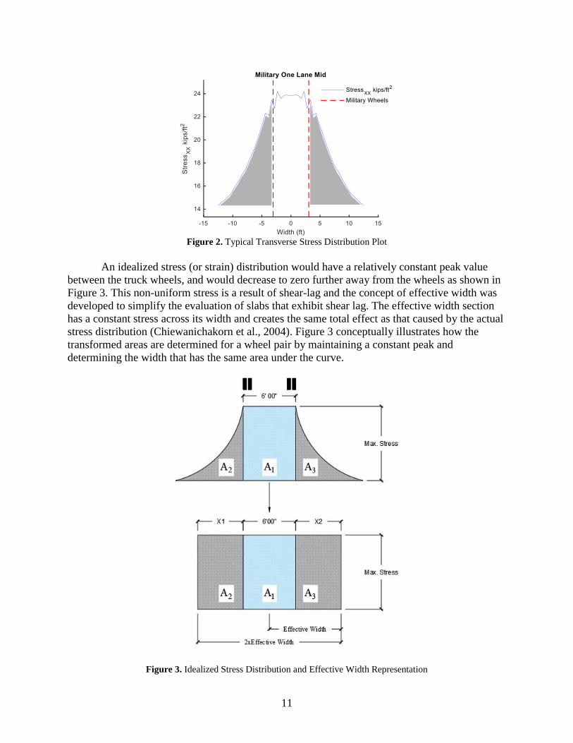
11

Figure 2. Typical Transverse Stress Distribution Plot

An idealized stress (or strain) distribution would have a relatively constant peak value

between the truck wheels, and would decrease to zero further away from the wheels as shown in

Figure 3. This non-uniform stress is a result of shear-lag and the concept of effective width was

developed to simplify the evaluation of slabs that exhibit shear lag. The effective width section

has a constant stress across its width and creates the same total effect as that caused by the actual

stress distribution (Chiewanichakorn et al., 2004). Figure 3 conceptually illustrates how the

transformed areas are determined for a wheel pair by maintaining a constant peak and

determining the width that has the same area under the curve.

Figure 3. Idealized Stress Distribution and Effective Width Representation

12

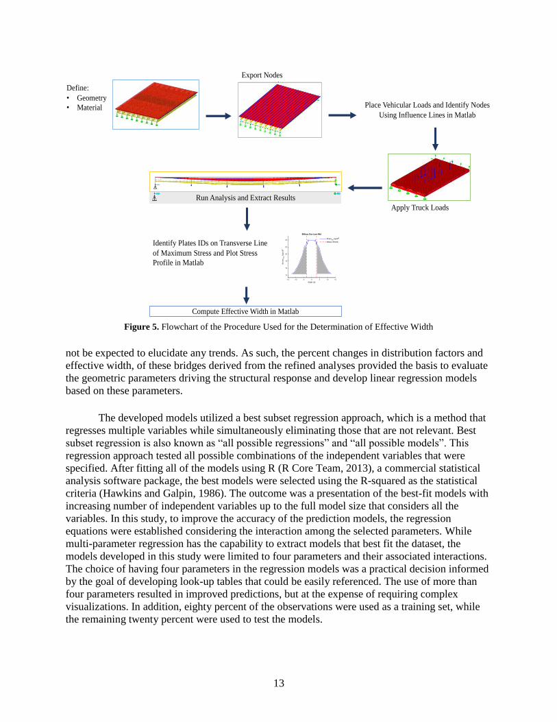
Process Automation

Initially, the bridge geometry including section properties were specified in LARSA 4D

(LARSA, Inc.). A mesh was generated based on the dimensions of the bridge as well as taking

into consideration the computational time and the application of load. To apply the truck loads

and minimize the amount of finite element data required, a MATLAB (Mathworks, Inc.) script

was developed. A database with the axle loads of common trucks was identified and generated in

MATLAB. The MATLAB script had two main tasks: (1) read and identify the nodes associated

with the truck loading for each truck and (2) write a modified LARSA 4D file with the applied

loads for each scenario. Finally, the analysis was conducted using the modified LARSA 4D file,

and the results were extracted for each case. For the girder and slab bridges, a flowchart of the

procedure for determining the load distribution factor and effective width is shown in Figures 4

and 5, respectively.

Figure 4. Flowchart of the Procedure Used for the Determination of the Live Load Distribution Factor

The AASHTO trucks considered in the analyses were the HL93-Design Tandem, the HL-

93/HS20-44 Design Truck, and the SU7 Legal Truck. A number of load cases needed to be

tested in the longitudinal and transverse positions to determine the maximum effect generated at

a specific location using the selected trucks. The truck positions that produced the maximum

moment and shear in the longitudinal direction were first determined. Then, three transverse

positions were considered for both moment and shear effects: (1) a truck placed 2 ft from the

curb of the parapets; (2) a truck placed at the quarter length of the clear road width; and (3) a

truck placed in the mid-transverse position of the bridge. The same was repeated for two trucks.

Therefore, a total of 36 load cases were considered for each bridge.

Prediction Models

Results derived from the refined methods of analysis provided the foundation describing

the characteristics that influenced the load sharing behavior within the selected bridge categories.

With a goal of understanding where potential improvements in rating factor could be achieved,

an understanding of the bridge parameters driving this load sharing behavior was necessary.

However, the pool of bridges was limited to around 20 to 25 bridges per category, which would

Apply Truck Loads

Export Nodes

Define:

• Geometry

• Material Place Vehicular Loads and Identify Nodes

Using Influence Lines in Matlab

Compute Load Distribution Factor using Load Fraction

Analysis in Matlab

Run Analysis and Extract Results

13

Figure 5. Flowchart of the Procedure Used for the Determination of Effective Width

not be expected to elucidate any trends. As such, the percent changes in distribution factors and

effective width, of these bridges derived from the refined analyses provided the basis to evaluate

the geometric parameters driving the structural response and develop linear regression models

based on these parameters.

The developed models utilized a best subset regression approach, which is a method that

regresses multiple variables while simultaneously eliminating those that are not relevant. Best

subset regression is also known as “all possible regressions” and “all possible models”. This

regression approach tested all possible combinations of the independent variables that were

specified. After fitting all of the models using R (R Core Team, 2013), a commercial statistical

analysis software package, the best models were selected using the R-squared as the statistical

criteria (Hawkins and Galpin, 1986). The outcome was a presentation of the best-fit models with

increasing number of independent variables up to the full model size that considers all the

variables. In this study, to improve the accuracy of the prediction models, the regression

equations were established considering the interaction among the selected parameters. While

multi-parameter regression has the capability to extract models that best fit the dataset, the

models developed in this study were limited to four parameters and their associated interactions.

The choice of having four parameters in the regression models was a practical decision informed

by the goal of developing look-up tables that could be easily referenced. The use of more than

four parameters resulted in improved predictions, but at the expense of requiring complex

visualizations. In addition, eighty percent of the observations were used as a training set, while

the remaining twenty percent were used to test the models.

Apply Truck Loads

Export Nodes

Define:

• Geometry

• Material Place Vehicular Loads and Identify Nodes

Using Influence Lines in Matlab

Run Analysis and Extract Results

Compute Effective Width in Matlab

Identify Plates IDs on Transverse Line

of Maximum Stress and Plot Stress

Profile in Matlab

14

Comparison with AASHTO LRFD Bridge Design Specifications

For all analyses, comparisons of performances are described relative to the design

reference of the AASHTO LRFD Bridge Design Specifications. More specifically, for girder

bridges, AASHTO LRFD lateral load distribution factors for moment and shear served as the

references for comparison, while the effective width defined in the AASHTO LRFD

specifications served as the reference for slab bridges. The distribution factors for moment and

shear for the exterior and interior girders and the effective width for slab bridges were computed

from the refined analyses and compared with those computed using the AASHTO LRFD

equations. For girder bridges, based on the results of the analysis for each bridge within the

evaluation population, the cumulative worst case (i.e. largest distribution factor) were compared

with the AASHTO LRFD design reference as a percent change using Equation 3,

where:

DFmodel = the load distribution factor (DF) computed using refined analysis

DFAASHTO = the DF computed from the AASHTO LRFD Specifications

DF = the percent change in the DF when computed using refined analysis versus the

AASHTO LRFD specifications.

Note that a negative change indicates that the refined analysis method showed a bridge with the

given parameters was more effective in distributing the load than originally predicted and thus

yielded an improvement in the load rating relative to the AASHTO LRFD design basis.

For slab bridges, the smallest effective width obtained for either single lane loading or

multi-lane loading cases was compared with the effective width computed using the

corresponding AASHTO LRFD equation as a percentage change using Equation 4,

∆EW (%) =EWmodel − EWAASHTO

EWAASHTO

∙ 100 (4)

where:

EWmodel = the effective width (EW) computed using refined analysis

EWAASHTO = EW computed using AASHTO LRFD Specifications

EW = the percent change in the DF when computed using refined analysis versus the

AASHTO LRFD specifications.

Note that a positive change in effective width indicates an improvement in the rating factor for

slab bridges. The results of changes in effective width are presented for single and multi-lane

loading cases separately for slab bridges analyzed through refined analysis methods. However,

the results from the worst loading case, i.e. smallest effective width computed for single and

multi-lane loading cases, were considered in the development of prediction models.

∆DF (%) =DFmodel − DFAASHTO

DFAASHTO

∙ 100 (3)

15

As can be seen from the load rating equation provided in Equation 1, the rating factor is

inversely proportional to the distribution factor. Therefore, taking all the variables except the

distribution factor in the load rating equation as the same, the percent change in the rating factor

(RF) computed from refined analysis versus that from the AASHTO LRFD Specifications can

be obtained as:

∆RF (%) =RFmodel − RFAASHTO

RFAASHTO

∙ 100 = (RFmodel

RFAASHTO

− 1) ∙ 100 (5)

or

∆RF (%) = (𝐷FAASHTO

DFmodel

− 1) ∙ 100 (6)

where, RFmodel and RFAASHTO denote the rating factor computed using refined analysis and

AASHTO LRFD Specifications, respectively.

RESULTS AND DISCUSSION

Literature Review

This literature review is organized into two main sections. First, the review of the

literature on the use of refined analysis methods in evaluation of load distribution factors and

bridge load rating is provided. Then, the impacts of the SHVs and EVs on the load rating process

are reviewed.

Refined Analysis for Load Distribution and Load Rating

The analytical expressions to determine the load distribution factors in the AASHTO

LRFD Specification were developed as a result of NCHRP 12-26 project (Zokaei, 1991), where

extensive parametric studies on straight, single-span bridges were conducted using finite element

analysis. The results from the study were considered as a better representation of load

distribution in bridge structures compared to “S-over” equations in the AASHTO Standard

Specification. However, AASHTO LRFD formulas were developed by making a set of

assumptions and therefore have some limitations. For instance, the girder spacing was assumed

to be uniformly distributed and all girder characteristics were taken to be the same. It was also

assumed that the HS-20 design vehicle governed the distribution behavior. In addition, the

effects of some important parameters such as cross-frames, diaphragms, and deck cracking in

load distribution were not considered in the development of these expressions.

Since the development of AASHTO LRFD load distribution expressions, a number of

studies have been conducted to investigate load distribution behavior of girder bridges and slab

bridges through refined analysis. These studies evaluated the effects of various parameters on the

load distribution factors and compared their findings with the AASHTO Standard and LRFD

approaches. These studies highlight the current state of practice regarding the application of

16

refined methods of analysis to better describe load sharing behavior, but also emphasize the

variability of impact of bridge parameters on these same behaviors.

Girder Bridges

Chung et al. (2006) investigated the influence of cross bracings, parapets, and deck

cracking on load distribution factors of steel girder bridges. They developed 3D finite element

models of 9 in-service bridges in Indiana using ABAQUS. Shell elements were used to model

the concrete deck, while the steel girders and bracing elements were modeled using beam

elements. The composite action between the girder and deck was modeled by rigid links. The

models were loaded with the AASHTO HS20 design truck to obtain the live load distributions.

The study found that when the load distribution factors were calculated using finite element

models that consider lateral bracings, the factors decreased by up to 11% compared to those

computed using finite element models that included only primary members. A decrease up to

25% was observed when only parapets were considered in the models. When both lateral bracing

and parapets were added to the models, the load distribution factors were 17-38% less than those

obtained using the models with only primary members. On the other hand, considering

longitudinal cracks on the concrete deck increased the load distribution factors by 17% while the

transverse cracks had a negligible effect on the load distribution behavior.

Harris (2010) comparatively evaluated a number of methods used by researchers to

determine load distribution factors for girder bridges. The load distribution factors were

computed using an approach based on either the load fraction method or the beam-line method.

The finite element model of a bridge validated through the field-testing results was used to

determine member response including strains, deflections, and moments, which were then used

to determine load distribution factors using variations of the load fraction and beam-line

methods. The results demonstrated that both of these methods were effective for determining

load distribution factors, but proper selection and use of appropriate member response variables

was critical.

Catbas et al. (2012) developed 3D finite element models of 40 reinforced concrete (RC)

T-beam bridges and evaluated the load distribution factor by analyzing the moment values under

HL-93 design truck loads. The models included 3D solid elements for concrete and frame

elements for reinforcing bars. The effects of secondary elements such as diaphragms, parapets,

and sidewalks were not considered. The study found interior girder moment demands decreased

at least 30% when they were computed through finite element analysis rather than AASHTO

LRFD equations. The authors proposed a method to compute the load distribution factors using

parameters obtained from a simple dynamic test and measured skew angle. Field testing on four

in-service T-beam bridges was conducted to evaluate the load distribution factors through both

the proposed approach and the detailed field-calibrated finite element models. The rating factors

for these bridges were also computed using the AASHTO LRFD approach. The average ratio of

the load ratings computed by fully calibrated models to AASHTO load ratings was 3.32, while

the average ratio of the load rating estimated by the proposed approach to AASHTO load ratings

was 1.40. These outcomes demonstrated the potential benefits derived from the proposed

approach, which still resulted in improved rating factors compared to AASHTO approach while

remaining conservative compared to the fully calibrated finite element modeling approach.

17

Nouri and Ahmedi (2012) assessed the effect of skew angle on the load distribution

behavior of continuous two-span steel girder bridges. They performed finite element analysis of

72 bridges with varying parameters under AASHTO HS-20 loading in SAP 2000. The models

employed shell elements for concrete deck, beam elements for girders, and rigid link elements to

connect shell and beam elements for representing the composite action between the deck and

girders. The results showed that the moment demands for interior and exterior girders decreased

up to 33% when the skew angle varied from 0 to 45. The shear forces at the pier support

decreased for interior girders, but increased for exterior girders with increasing skew angle. The

study also concluded that the AASHTO LRFD approach overestimated the moment and shear

distribution factors up to 45% when the skew angle was over 20.

Snyder and Beisswenger (2017) studied shear rating factors for prestressed concrete

beams using refined analysis in a project funded by Minnesota DOT. They analyzed 50

prestressed concrete bridges through 2D grillage models and computed the live load distribution

factors considering the location-based load distribution of each axle along the span. They found

an average of 7% decrease in live load distribution factors. This refined analysis increased load

ratings for all of the analyzed bridges by an average of 16%.

Dymond et al. (2019) conducted a parametric study to evaluate the shear distribution

factors for prestressed concrete girder bridges without any skew. They found that the ratio of

longitudinal stiffness (composite girder longitudinal moment of inertia divided by cube of span

length) to transverse stiffness (transverse deck strip moment of inertia divided by cube of beam

spacing) plays an important role in shear distributions. They reported that when the stiffness ratio

was less than 1.5, the live load shear demands calculated by refined analysis were lower than

those computed by the AASHTO LRFD approach, while the refined analysis and AASHTO

approximation lead to similar results if the stiffness ratio was between 1.5 and 5.0. However, the

refined analysis produced higher shear demands for bridges with a stiffness ratio greater than 5.0.

Slab Bridges

Amer et al. (1999) conducted a parametric study to assess the influence of span length,

bridge width, slab thickness, and edge beams on the effective width of solid slab bridges. A basic

grid analysis approach was used to model 27 slab bridges with varying parameters. The models

were loaded with the AASHTO HS20 design truck. They concluded that the span length and

edge beams were the main parameters that influenced the effective width. The effective widths

computed by grillage analysis were always higher than those computed with the AASHTO

LRFD approach. Three bridges were experimentally tested and the effective width for each

bridge was computed based on measured strains. Results indicated that the effective width of

these bridges computed by grillage analysis was 14% higher on average than those computed by

AASHTO equations, while the effective widths based on field tests were 40% higher on average

than AASHTO effective width calculations. Therefore, while the AASHTO calculations were

the most conservative, the proposed methods were about 25% more conservative than what has

been observed in actual load tests.

Mabsout et al. (2004) studied the load distribution behavior of single span, simply-

supported reinforced concrete slab bridges through parametric analysis. Finite element analyses

of 112 bridges with varying span lengths, number of lanes, slab thickness, and edge condition

18

were performed using SAP 2000. The models used shell elements to represent the concrete slab.

Various loading conditions were considered using the AASHTO design truck. The maximum

longitudinal moments obtained from the models were compared with those computed through

AASHTO Standard and LRFD Specifications. They concluded that the AASHTO LRFD

Specification overestimated the bending moments for slab bridges.

Jauregui et al. (2007) investigated the load distribution behavior of an in-service RC

continuous slab bridge in a project funded by the New Mexico DOT. A finite element model of

the bridge was developed in SAP 2000 using shell elements to model the slab. The model was

validated using strain measurements obtained from a diagnostic load test. They found that the

effective width increased by 26% and 22% for positive moment and 13% and 11% for negative

moment for the exterior and interior spans, respectively, compared to the AASHTO LRFD

approach.

Davids et al. (2013) conducted refined analysis of 14 in-service slab bridges maintained

by the Maine DOT. The analyses were performed using a finite element analysis software,

SlabRate, developed and validated by the researchers. The software employed quadratic plate

elements to model the slab. The finite element analyses resulted in an average of 25.5%, 25.7%,

and 26.3% increase in rating factors for the HL-93 truck, HL-93 tandem, and AASHTO notional

load, respectively, compared to the AASHTO LRFD approach.

Impacts of SHVs and EVs on Bridge Load Rating

There have been only a few published studies related to the effects of SHVs and/or EVs

on bridge load ratings. Islam (2018) discussed a study where 187 in-service bridges owned by

Ohio DOT were load rated by either load factor rating or load and resistance factor rating for

both Ohio legal trucks and SHVs. The bridges selected for the study included concrete slab

bridges, prestressed concrete I-girder and box-girder bridges, and steel girder bridges. The results

showed that almost all of the evaluated bridges that had an RF greater than 1.35 for Ohio legal

loads also had an RF greater than 1.00 for SHV loads.

Selection of the Population of Structures to Be Evaluated

After applying filters to focus on only highway bridges, there were a total of 11,440

bridges in the database obtained from VDOT. Figure 6 (a) shows the distribution of bridges with

an RF < 1.0 for either inventory rating or when they are rated with SU trucks, for each of three

route types. The RF values are grouped into four ranges: (i) < 0.3, (ii) 0.3 – 0.5, (iii) 0.5 – 0.7,

and (iv) 0.7 – 1.0. 81% of the bridges with a RF < 1.0 are located along secondary routes. For

those secondary route bridges, 49% of bridges had an RF below 0.7. 89% of primary route

bridges and all interstate bridges with an RF < 1.0 had an RF over 0.7. Figure 6 (b) shows the

distribution of all bridges with an RF < 1.0 based on structural type. It can be seen that most of

the bridges were categorized as girder bridges (74%) and slab bridges (22%).

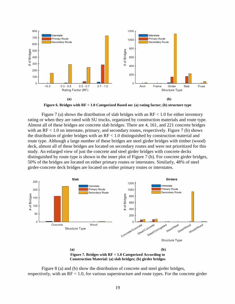
19

Figure 6. Bridges with RF < 1.0 Categorized Based on: (a) rating factor; (b) structure type

Figure 7 (a) shows the distribution of slab bridges with an RF < 1.0 for either inventory

rating or when they are rated with SU trucks, organized by construction materials and route type.

Almost all of these bridges are concrete slab bridges. There are 4, 161, and 221 concrete bridges

with an RF < 1.0 on interstate, primary, and secondary routes, respectively. Figure 7 (b) shows

the distribution of girder bridges with an RF < 1.0 distinguished by construction material and

route type. Although a large number of these bridges are steel girder bridges with timber (wood)

deck, almost all of these bridges are located on secondary routes and were not prioritized for this

study. An enlarged view of just the concrete and steel girder bridges with concrete decks

distinguished by route type is shown in the inner plot of Figure 7 (b). For concrete girder bridges,

50% of the bridges are located on either primary routes or interstates. Similarly, 48% of steel

girder-concrete deck bridges are located on either primary routes or interstates.

Figure 7. Bridges with RF < 1.0 Categorized According to

Construction Material: (a) slab bridges; (b) girder bridges

Figure 8 (a) and (b) show the distribution of concrete and steel girder bridges,

respectively, with an RF < 1.0, for various superstructure and route types. For the concrete girder

20

bridges, 68% of the bridges are reinforced concrete T-beam bridges. 53% of these T-beam

bridges are located on primary routes, while 45% are on the secondary routes. For steel girder

bridges, 69% are simple span girder bridges. About 3% of these simple span steel bridges are

located on the interstate routes while the remaining bridges are equally distributed on the primary

and secondary routes.

Figure 8. Girder Bridges with RF < 1.0 Categorized Based on Superstructure Type: (a) concrete girder

bridges; (b) steel girder bridges

Based on the above findings, three bridge classes were selected for the assessment of

their load distribution behavior using refined analysis: (1) steel girder bridges; (2) reinforced

concrete T-beam bridges; and (3) concrete slab bridges. For each of these bridge classes, the

database of bridges with an RF < 1.0 was further analyzed to select representative bridges for

each bridge class. In particular, the statistics of span length, number of lanes, and skew angle

were analyzed for each bridge class. Although it was desirable to initially classify girder bridges

also based on girder spacing and slab bridges based on slab thickness, this information was not

available in the database.

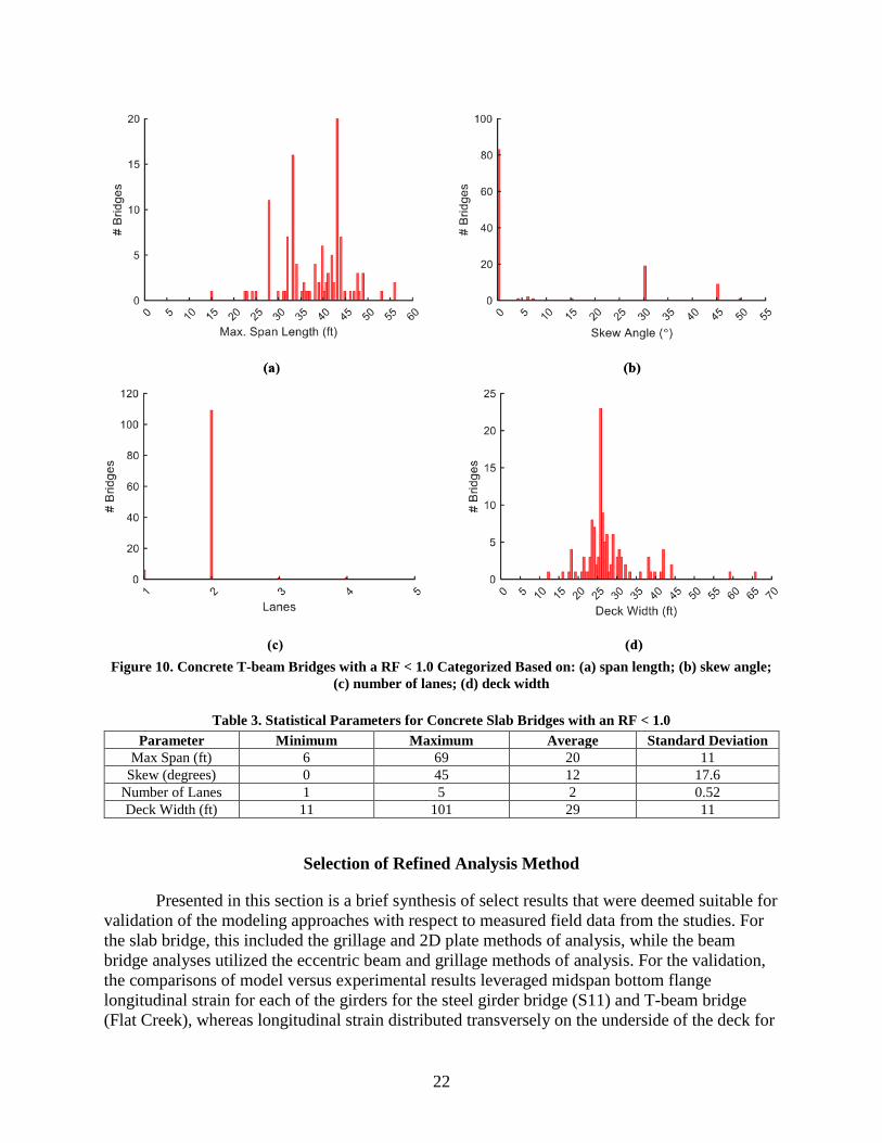
Figures 9—11 show the distribution of steel girder bridges, concrete T-beam bridges, and

slab bridges, respectively, based on span length, number of lanes, deck width, and skew angle.

The summary of the statistical distributions is also provided in Tables 1—3. The average

maximum span lengths for the steel girder, concrete T-beam, and slab bridges were 48.0 ft, 37.9

ft, and 20.0 ft, respectively. For the steel girder bridges, more than 90% of the bridges were non-

skewed. For the concrete T-beam and slab bridges, most of the bridges were also non-skewed,

but there were about 24% bridges with a skew angle of 30 or 45. Two-lane bridges were the

most common for all bridge classes and the average deck widths were about 28-29 ft.

Based on the above statistical distributions for each bridge class, population pools of 21,

25, and 25 bridges were selected for the refined analyses for the steel girder, concrete T-beam,

and slab bridges, respectively. The selection was limited to 21-25 bridges due to the manual

nature of the bridge plan acquisitions, structural detail extraction from those plans, and manual

entry of relevant geometry required to develop the models. In the selection of bridges, a priority

was also given to bridges located on interstate and primary routes. Additionally, some iteration

21

Figure 9. Steel Girder Bridges with a RF < 1.0, Categorized Based on: (a) span length; (b) number of lanes;

(c) skew angle; (d) rating

on the selected pool was required because the details of the bridge geometries were only

completely available after reviewing plans and the goal was to develop a pool that was

geometrically representative of the population. Tables 4—6 provide the main properties of the

selected bridges for the steel girder, concrete T-beam, and slab bridges, respectively.

Table 1. Statistical Parameters for Steel Girder Bridges with an RF < 1.0

Parameter Minimum Maximum Average Standard Deviation

Max Span (ft) 7 153 48 24.5

Skew (degrees) 0 60 8 14.5

Number of Lanes 1 9 2 1

Deck Width (ft) 12 148 28 18

Table 2. Statistical Parameters for Concrete T-Beam Bridges with an RF < 1.0

Parameter Minimum Maximum Average Standard Deviation

Max Span (ft) 15 56 37.9 7.2

Skew (degrees) 0 50 9 15.7

Number of Lanes 1 4 2 0.3

Deck Width (ft) 12 66 27.9 7.4

22

Figure 10. Concrete T-beam Bridges with a RF < 1.0 Categorized Based on: (a) span length; (b) skew angle;

(c) number of lanes; (d) deck width

Table 3. Statistical Parameters for Concrete Slab Bridges with an RF < 1.0

Parameter Minimum Maximum Average Standard Deviation

Max Span (ft) 6 69 20 11

Skew (degrees) 0 45 12 17.6

Number of Lanes 1 5 2 0.52

Deck Width (ft) 11 101 29 11

Selection of Refined Analysis Method

Presented in this section is a brief synthesis of select results that were deemed suitable for

validation of the modeling approaches with respect to measured field data from the studies. For

the slab bridge, this included the grillage and 2D plate methods of analysis, while the beam

bridge analyses utilized the eccentric beam and grillage methods of analysis. For the validation,

the comparisons of model versus experimental results leveraged midspan bottom flange

longitudinal strain for each of the girders for the steel girder bridge (S11) and T-beam bridge

(Flat Creek), whereas longitudinal strain distributed transversely on the underside of the deck for

23

Figure 11. Concrete Slab Bridges with a RF < 1.0 Categorized Based on: (a) span length; (b) skew angle; (c)

number of lanes; (d) deck width

the slab bridge (Smacks Creek). Results for these comparisons are illustrated in Figures 12—14.

When comparing the results across all three bridges, the models were clearly able to describe the

behavior characteristics with corresponding relative responses within the system.

For both the Flat Creek and Smacks Creek bridges, the eccentric beam and 2D plate

formulations, respectively, agreed not only in behavior characteristics, but also magnitude of

derived response with respect to experimental data. For the same structures, the grillage

approach exhibited less agreement with respect to magnitude with apparent higher distributions

within the system.

For the S11 bridge, in addition to field test results of the Eom and Nowak (2001) study,

numerical results for the pin–roller scenario provided in the same study was also compared with

the modelling approaches (grillage and eccentric beam) in the current study, without any attempt

to calibrate the rotational restraint of the supports. This approach was adopted since the intent of

24

Table 4. Steel Girder Bridges Selected for Refined Analysis

No. Bridge Key Route

Span

Length

(ft)

Girder

Spacing

(ft)

Overall

Section

Depth (in)

Skew

Angle

(degrees)

Deck

Width

(ft)

Number

of Lanes

1 10370 Primary 40.5 7.7 36.7 30 24.0 2

2 10711 Primary 92.5 8.3 44.6 0 26.0 2

3 11884 Primary 47.5 6.8 40.6 0 28.0 2

4 12165 Primary 61.0 10.0 71.3 0 42.7 3

5 12641 Primary 54.8 7.2 40.7 23 44.0 3

6 13273 Interstate 96.0 6.3 40.3 0 20.0 2

7 14852 Primary 83.8 9.0 44.1 37 56.0 4

8 18185 Primary 26.0 5.8 27.9 0 24.0 2

9 18928 Secondary 45.3 9.0 34.9 28 47.0 3

10 19596 Secondary 54.0 7.7 40.3 7 30.8 2

11 20201 Primary 72.5 6.5 42.9 79 39.0 2

12 20547 Primary 75.9 7.3 42.9 68 38.8 3

13 2432 Primary 42.5 7.5 36.8 45 24.0 2

14 24482 Primary 110.0 9.0 65.0 0 30.0 2

15 2621 Primary 55.0 6.8 40.3 0 27.8 2

16 356 Primary 32.5 7.7 34.4 0 26.0 2

17 4398 Primary 70.0 6.3 42.9 0 26.0 2

18 5792 Primary 85.0 6.8 44.9 0 34.8 2

19 7089 Interstate 106.5 7.9 65.0 0 66.6 5

20 7758 Primary 42.8 4.3 28.2 0 18.0 1

21 9371 Primary 70.9 6.6 43.4 0 28.0 2

the investigation was to judge performance of various methods for determining lateral load

distribution instead of an exercise in model calibration. For this bridge, the grillage and eccentric

beam formulations aligned better, but exhibited a departure from the experimental data. This

departure is attributed to the effects of boundary conditions, which were shown from the Eom

and Nowak (2001) study to exhibit a higher level of restraints than idealized models, thus

resulting in lower (that is, more conservative) strain values than the idealized simple support

models. Note that the results obtained from grillage and eccentric beam models of the current

study aligned well with the numerical results obtained in Eom and Nowak (2001) study, where a

pin-roller support assumption was also made.

Based on the results derived from these validations and other loading scenarios, the

modeling approaches were both deemed suitable for continued study. While both sets of

approaches (eccentric beam/grillage and 2D plate/grillage) proved effective, the eccentric beam

and 2D plate analysis approaches provided an additional benefit due to model development

efficiency within the LARSA 4D software package. Note that, for the eccentric beam analysis,

LARSA 4D allows generating models automatically with little effort using built-in templates that

can also be modified using spreadsheets. On the other hand, the grillage analysis in LARSA 4D

requires additional efforts for the placement of grid lines and the calculations of some sectional

properties, such as bending and torsional inertias. Therefore, the eccentric beam and 2D plate

analysis approaches were used for the remainder of the study.

25

Table 5. Concrete T-beam Bridges Selected for Refined Analysis

No. Bridge

Key Route

Span

Length

(ft)

Girder

Spacing (ft)

Overall

Section

Depth (in)

Skew

Angle

(degrees)

Deck

Width

(ft)

Number

of

Lanes

1 1210 Primary 27.9 6.0 25.0 30 27.2 2

2 12384 Primary 34.1 9.6 35.6 30 31.0 2

3 12417 Primary 47.9 7.9 28.0 50 26.1 2

4 13184 Secondary 23.0 6.0 28.0 0 25.8 2

5 13867 Secondary 40.3 7.2 37.0 0 25.5 2

6 14023 Primary 40.0 6.0 36.3 0 36.8 2

7 15402 Secondary 40.0 9.0 36.4 0 20.4 2

8 15533 Secondary 40.0 7.2 39.0 0 27.9 2

9 16565 Primary 44.0 7.2 39.0 45 30.1 2

10 16566 Primary 44.0 7.2 39.0 45 26.2 2

11 1709 Primary 32.2 10.0 31.1 0 25.4 2

12 17237 Secondary 44.0 8.0 35.9 0 19.1 2

13 17757 Primary 32.0 9.0 31.4 0 22.5 2

14 18493 Primary 28.0 7.2 32.0 30 24.1 2

15 1892 Primary 26.0 6.0 25.0 30 28.3 2

16 2430 Primary 43.0 7.7 45.0 30 23.8 2

17 4357 Primary 24.9 5.1 32.1 0 23.8 4

18 4850 Primary 36.5 7.8 33.3 0 31.3 2

19 5100 Primary 45.9 7.6 39.6 45 27.1 2

20 7770 Primary 47.9 6.5 40.5 0 34.5 2

21 8022 Secondary 22.5 5.7 29.0 0 38.4 2

22 8690 Primary 42.5 7.2 26.8 0 26.0 2

23 912 Primary 43.0 7.6 41.9 45 30.8 2

24 9161 Primary 44.7 7.8 43.0 0 47.3 2

25 9317 Secondary 48.1 8.0 39.6 0 44.3 2

Figure 12. Model Validation for Steel Girder Bridge (S11 Bridge)

26

Table 6. Concrete Slab Bridges Selected for Refined Analysis

No. Bridge Key Route Span

Length (ft)

Skew Angle

(degrees)

Deck Width

(ft)

Section

Depth (in)

Number

of Lanes

1 391 Secondary 18.0 0 25.5 17.5 2

2 10588 Primary 20.0 0 25.5 19.0 2

3 21217 Primary 22.5 0 59.4 20.0 2

4 9107 Secondary 40.0 0 29.8 17.0 2

5 7855 Secondary 40.0 0 28.9 20.0 2

6 19539 Primary 22.0 10 36.0 18.5 2

7 3414 Secondary 15.1 5 25.9 15.0 2

8 3416 Secondary 14.1 15 25.9 14.0 2

9 26888 Secondary 54.0 15 28.0 20.0 2

10 2633 Primary 15.1 30 49.9 14.0 2

11 4361 Primary 20.0 30 77.1 19.0 2

12 18127 Secondary 40.0 30 26.9 20.0 2

13 5511 Secondary 17.1 35 22.0 17.5 4

14 3173 Primary 23.0 45 46.9 18.0 2

15 18900 Primary 20.0 45 28.0 15.0 2

16 13198 Primary 14.1 45 25.9 14.0 2

17 18840 Primary 23.0 0 25.5 22.0 4

18 13230 Primary 23.0 0 25.5 22.0 2

19 4545 Primary 23.0 0 25.5 19.5 2

20 10249 Primary 14.1 0 26.0 21.0 2

21 1870 Primary 14.1 0 25.5 21.0 2

22 18881 Primary 20.0 30 25.0 20.5 2

23 1185 Primary 24.0 30 26.3 16.0 2

24 17401 Primary 14.0 45 25.0 18.5 2

25 17694 Primary 23.0 45 17.5 17.5 2

Figure 13. Model Validation for RC T-beam Bridge (Flat Creek Bridge)

27

Figure 14. Model Validation for Concrete Slab Bridge (Smacks Creek Bridge)

Refined Analysis of Bridge Classes and Evaluation of Load Distribution Behavior

Results from Modeled Bridges

For the 21 steel girder bridges, 25 reinforced concrete T-beam bridges, and 25 reinforced

concrete slab bridges, the relative performance of the refined methods of analyses are presented

in Tables 7—9, respectively. As shown in each of these tables, the change in distribution factors

(DF) and load rating factors (RF) are typically inversely proportional. Also, note that the

change in effective width (EW) is directly proportional to the load rating factor, i.e., an increase

in the effective width will lead to an increased rating factor.

Prediction Models

A series of multi-parameter linear regression models were developed to predict the

percent change in distribution factor for slab-on-girder bridges and percent change in effective

width for slab bridges using four variables that described the geometrical characteristics of the

bridges. Although all regression models use four variables, these variables differ in each model

and were selected based on their significance in a given scenario. Also, note that the developed

regression models and corresponding tables are reliable for the parameter space presented in

each table. Each of the regressions models developed was validated through a comparison of the

predictions to the results derived from the refined analyses.

The following notation applies to all of the prediction model equations and tables:

d = depth of beam or stringer (in.)

L = span of beam (ft)

Nb = number of beams, stringers, or girders

S = spacing of beams or webs (ft)

ts = depth of concrete slab (in.)

W = edge-to-edge width of bridge (ft)

I = moment of inertia of beam (in4)

θ = skew angle (degrees)

28

Table 7. Distribution and Load Rating Factors for Steel Girder Bridges – Refined Analyses Versus LRFD

Bridge

No.

Interior Moment Exterior Moment Interior Shear Exterior Shear

DF RF DF RF DF RF DF RF

1 -6% 6% 0% 0% 6% -6% -5% 5%

2 -2% 2% -11% 12% 9% -8% -2% 2%

3 -10% 11% -50% 100% 13% -12% -53% 113%

4 -22% 28% -33% 49% 31% -24% -12% 14%

5 -20% 25% -22% 28% 8% -7% -21% 27%

6 0% 0% 0% 0% 0% 0% 6% -6%

7 -14% 16% 7% -7% 10% -9% -26% 35%

8 -17% 20% -29% 41% 3% -3% -30% 43%

9 -18% 22% -17% 20% -4% 4% -24% 32%

10 20% -17% -32% 47% -14% 16% -48% 92%

11 -37% 59% -26% 35% 15% -13% -54% 117%

12 -19% 23% -11% 12% 2% -2% -28% 39%

13 1% -1% -14% 16% 7% -7% -7% 8%

14 -2% 2% -16% 19% 24% -19% -7% 8%

15 -7% 8% -52% 108% 13% -12% -55% 122%

16 -2% 2% -26% 35% -2% 2% -10% 11%

17 4% -4% -38% 61% 18% -15% -48% 92%

18 -12% 14% 24% -19% 12% -11% 81% -45%

19 -31% 45% -26% 35% -7% 8% 10% -9%

20 0% 0% 0% 0% 0% 0% 0% 0%

21 -4% 4% -51% 104% 13% -12% -41% 69%

Table 8. Distribution and Load Rating Factors for T-Beam Bridges – Refined Analyses Versus LRFD

Bridge

No.

Interior Moment Exterior Moment Interior Shear Exterior Shear

DF RF DF RF DF RF DF RF

1 6% -6% -43% 75% 4% -4% -25% 33%

2 -68% 213% 90% -47% -1% 1% 13% -12%

3 15% -13% -18% 22% -2% 2% -34% 52%

4 20% -17% -42% 72% 26% -21% -33% 49%

5 -21% 27% 62% -38% 12% -11% 55% -35%

6 -22% 28% -14% 16% 9% -8% 42% -30%

7 3% -3% -15% 18% 44% -31% -12% 14%

8 3% -3% -18% 22% 26% -21% 1% -1%

9 22% -18% -3% 3% 20% -17% -7% 8%

10 12% -11% 1% -1% 7% -7% 4% -4%

11 0% 0% -19% 23% 37% -27% -2% 2%

12 18% -15% -19% 23% 0% 0% 0% 0%

13 -4% 4% -18% 22% 43% -30% -9% 10%

14 10% -9% -16% 19% 26% -21% -15% 18%

15 -11% 12% -8% 9% -3% 3% -30% 43%

16 1% -1% 13% -12% 7% -7% 40% -29%

17 -12% 14% 0% 0% 11% -10% 24% -19%

18 -11% 12% -9% 10% 22% -18% -4% 4%

19 8% -7% 8% -7% 21% -17% 6% -6%

20 -8% 9% -1% 1% 4% -4% 25% -20%

21 -38% 61% 76% -43% 20% -17% 17% -15%

22 5% -5% 3% -3% 25% -20% 1% -1%

23 10% -9% 16% -14% 14% -12% 57% -36%

24 -25% 33% -27% 37% -7% 8% 10% -9%

25 -27% 37% -34% 52% 17% -15% -9% 10%

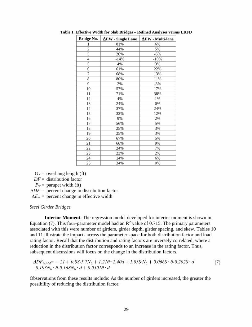
29

Table 1. Effective Width for Slab Bridges – Refined Analyses versus LRFD

Bridge No. EW - Single Lane EW - Multi-lane

1 81% 6%

2 44% 5%

3 26% -6%

4 -14% -10%

5 4% 3%

6 61% 22%

7 68% 13%

8 80% 11%

9 2% -8%

10 57% 17%

11 71% 38%

12 4% 1%

13 24% 0%

14 37% 24%

15 32% 12%

16 9% 2%

17 56% 5%

18 25% 3%

19 25% 3%

20 67% 5%

21 66% 9%

22 24% 7%

23 23% 2%

24 14% 6%

25 34% 0%

Ov = overhang length (ft)

DF = distribution factor

Pw = parapet width (ft)

∆DF = percent change in distribution factor

∆Ew = percent change in effective width

Steel Girder Bridges

Interior Moment. The regression model developed for interior moment is shown in

Equation (7). This four-parameter model had an R2 value of 0.715. The primary parameters

associated with this were number of girders, girder depth, girder spacing, and skew. Tables 10

and 11 illustrate the impacts across the parameter space for both distribution factor and load

rating factor. Recall that the distribution and rating factors are inversely correlated, where a

reduction in the distribution factor corresponds to an increase in the rating factor. Thus,

subsequent discussions will focus on the change in the distribution factors.

ΔDFint-M= − 21 + 0.8S-5.7Nb + 1.21θ+2.40d + 1.03S∙Nb + 0.066S ∙ θ-0.202S ∙ d

−0.193Nb ∙ θ-0.168Nb ∙ d + 0.0501θ ∙ d (7)

Observations from these results include: As the number of girders increased, the greater the

possibility of reducing the distribution factor.

30

Table 10. Percent Change in Distribution Factors for Interior Moment for Steel Girder Bridges

d = 25 30 35 40 45

Nb = 4 5 6 7 4 5 6 7 4 5 6 7 4 5 6 7 4 5 6 7

θ=0

S=6 -1 -5 -9 -13 1 -3 -8 -12 4 -2 -7 -12 6 0 -6 -12 9 2 -5 -12

S=7 -2 -4 -7 -10 0 -3 -7 -11 2 -3 -7 -11 3 -2 -7 -12 5 -1 -7 -13

S=8 -2 -3 -5 -7 -1 -4 -6 -9 -1 -4 -7 -11 0 -4 -8 -13 1 -4 -9 -14

S=9 -2 -2 -3 -4 -2 -4 -5 -7 -3 -5 -7 -10 -3 -6 -9 -13 -4 -8 -12 -16

θ=15

S=6 -6 -13 -20 -26 0 -8 -15 -22 6 -2 -10 -19 13 3 -6 -15 19 9 -1 -11

S=7 -6 -11 -17 -22 0 -7 -13 -19 5 -2 -9 -17 10 2 -6 -14 16 7 -2 -11

S=8 -5 -9 -14 -18 0 -6 -11 -17 4 -2 -8 -15 8 1 -6 -13 13 5 -3 -11

S=9 -4 -7 -11 -14 0 -5 -9 -14 3 -2 -8 -13 6 0 -6 -12 9 3 -4 -11

θ=30

S=6 -11 -21 -30 -40 -1 -12 -22 -32 9 -2 -14 -25 19 7 -5 -17 29 16 3 -10

S=7 -10 -18 -26 -35 0 -10 -19 -28 9 -2 -12 -22 18 7 -4 -15 27 15 3 -9

S=8 -8 -15 -23 -30 0 -8 -16 -24 8 -1 -10 -19 17 7 -3 -13 25 14 3 -8

S=9 -6 -12 -19 -25 1 -6 -13 -21 8 0 -8 -16 15 6 -3 -11 22 13 3 -7

θ=45

S=6 -16 -29 -41 -54 -3 -16 -29 -42 11 -3 -17 -31 25 10 -5 -20 39 23 7 -8

S=7 -14 -25 -36 -48 -1 -13 -25 -37 12 -1 -14 -27 25 11 -3 -17 38 23 8 -6

S=8 -11 -21 -31 -42 1 -10 -21 -32 13 1 -11 -23 25 12 -1 -14 37 23 9 -4

S=9 -8 -17 -26 -36 3 -7 -17 -28 14 3 -8 -19 25 13 1 -11 35 23 10 -3

θ = skew in the bridge, in degrees; S = girder spacing, in feet; d = girder depth, in inches; Nb = number of girders

Table 11. Percent Change in Rating Factors for Interior Moment for Steel Girder Bridges

d = 25 30 35 40 45

Nb = 4 5 6 7 4 5 6 7 4 5 6 7 4 5 6 7 4 5 6 7

θ=0

S=6 1 5 10 14 -1 3 9 14 -4 2 8 14 -6 0 7 14 -8 -2 6 14

S=7 2 4 7 11 0 4 8 12 -2 3 8 13 -3 2 8 14 -5 1 8 15

S=8 2 3 5 7 1 4 6 9 1 4 8 12 0 4 9 14 -1 5 10 17

S=9 2 2 3 4 2 4 5 7 3 5 8 11 3 7 10 14 4 8 13 18

θ=15

S=6 7 15 24 36 0 8 18 29 -6 2 11 23 -11 -3 6 17 -16 -8 1 12

S=7 6 12 20 29 0 7 15 24 -5 2 10 20 -9 -2 6 16 -14 -6 2 12

S=8 5 10 16 22 0 6 13 20 -4 2 9 17 -8 -1 6 15 -11 -4 3 13

S=9 4 8 12 17 0 5 10 16 -3 2 8 15 -6 0 6 14 -9 -2 5 13

θ=30

S=6 13 26 44 66 1 13 28 48 -8 2 16 33 -16 -6 5 21 -22 -14 -3 11

S=7 11 22 36 54 0 11 24 40 -8 2 13 28 -15 -6 4 18 -21 -13 -3 10

S=8 8 18 29 43 0 9 19 32 -8 1 11 23 -14 -6 4 15 -20 -12 -3 8

S=9 6 14 23 34 -1 6 15 26 -8 0 9 19 -13 -6 3 13 -18 -11 -3 7

θ=45

S=6 20 40 70 116 3 19 41 73 -10 3 20 45 -20 -9 5 24 -28 -19 -7 9

S=7 16 33 57 91 1 15 34 60 -11 1 16 37 -20 -10 3 20 -27 -19 -8 7

S=8 12 27 46 72 -1 11 27 48 -11 -1 12 30 -20 -11 1 16 -27 -19 -8 5

S=9 9 21 36 56 -3 8 21 38 -12 -3 9 24 -20 -11 -1 12 -26 -19 -9 3

θ = skew in the bridge, in degrees; S = girder spacing, in feet; d = girder depth, in inches; Nb = number of girders

31

Bridges with high skew angles had a higher chance of experiencing a reduction in

distribution factor when a refined analysis was conducted. For highly skewed bridges, the

largest reduction was associated with bridges that had a small girder depth and higher

number of girders.

As the girder depth increased, there was a lower probability of a reduction in the

distribution factor. For the bridges with a high girder depth and small number of girders,

even a small increase in the distribution factors can be observed.

Girder spacing had minimal effect on the change in distribution factors.

Exterior Moment. The regression model developed for exterior moment is shown in

Equation (8). This four-parameter model has an R2 value of 0.858. The primary parameters

associated with this model are girder depth, span length, skew angle, and slab thickness. Tables

12 and 13 illustrate the impacts across the parameter space for the distribution factor and load

rating factor, respectively.

ΔDFext-M = 358 + 2.43L − 51.4ts − 18.13d − 2.19θ − 0.018L∙ts − 0.0391L∙d

−0.0280L∙θ + 2.161ts.d + 0.098ts ∙ θ + 0.109d ∙ θ (8)

Observations from these results include:

As the slab thickness decreased, the distribution factors tended to be larger relative to the

AASHTO-calculated factors.

Table 12. Percent Change in Distribution Factors for Exterior Moment for Steel Girder Bridges

d = 25 30 35 40 45

ts = 7 8 9 7 8 9 7 8 9 7 8 9 7 8 9

θ=0

L=45 -29 -16 -3 -37 -24 -10 -44 -31 -18 -52 -39 -26 -59 -46 -33

L=55 -24 -11 3 -31 -18 -5 -39 -26 -13 -47 -33 -20 -54 -41 -27

L=65 -18 -5 8 -26 -13 0 -34 -20 -7 -41 -28 -15 -48 -35 -22

L=75 -13 0 13 -21 -7 6 -28 -15 -2 -36 -23 -9 -43 -30 -17

L=85 -8 6 19 -15 -2 11 -23 -10 4 -31 -17 -4 -38 -24 -11

θ=15

L=45 -26 -13 1 -34 -20 -7 -41 -28 -15 -49 -36 -22 -56 -43 -29

L=55 -21 -7 6 -28 -15 -2 -36 -23 -9 -43 -30 -17 -51 -37 -24

L=65 -15 -2 11 -23 -10 4 -30 -17 -4 -38 -25 -12 -45 -32 -19

L=75 -10 3 17 -17 -4 9 -25 -12 1 -33 -19 -6 -40 -27 -13

L=85 -4 9 22 -12 1 14 -20 -6 7 -27 -14 -1 -34 -21 -8

θ=30

L=45 -23 -9 4 -30 -17 -4 -38 -25 -11 -46 -32 -19 -53 -39 -26

L=55 -17 -4 9 -25 -12 2 -33 -19 -6 -40 -27 -14 -47 -34 -21

L=65 -12 1 15 -20 -6 7 -27 -14 -1 -35 -22 -8 -42 -29 -15

L=75 -7 7 20 -14 -1 12 -22 -9 5 -29 -16 -3 -37 -23 -10

L=85 -1 12 25 -9 4 18 -16 -3 10 -24 -11 2 -31 -18 -5

θ=45

L=45 -19 -6 7 -27 -14 -1 -35 -21 -8 -42 -29 -16 -49 -36 -23

L=55 -14 -1 12 -22 -8 5 -29 -16 -3 -37 -24 -10 -44 -31 -18

L=65 -9 5 18 -16 -3 10 -24 -11 3 -32 -18 -5 -39 -25 -12

L=75 -3 10 23 -11 2 16 -19 -5 8 -26 -13 0 -33 -20 -7

L=85 2 15 29 -6 8 21 -13 0 13 -21 -8 6 -28 -15 -1

θ = skew in the bridge, in degrees; L = span length, in feet; d = beam depth, in inches; ts = slab thickness, in inches

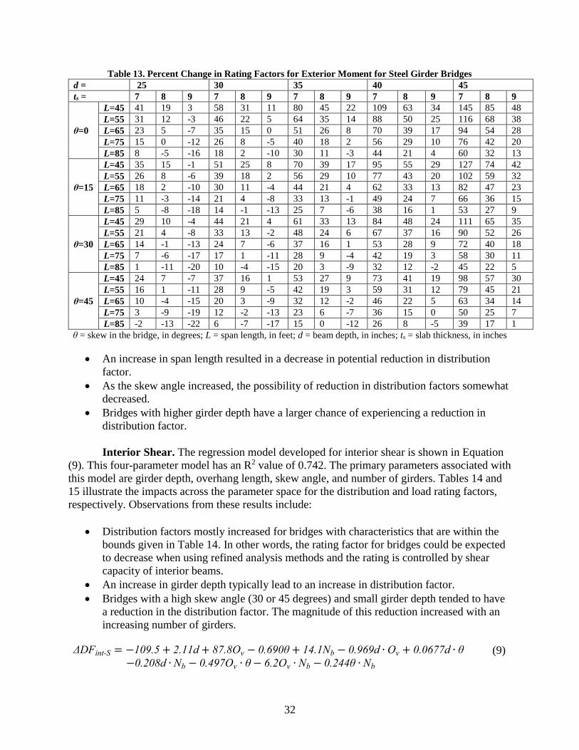
32

Table 13. Percent Change in Rating Factors for Exterior Moment for Steel Girder Bridges

d = 25 30 35 40 45

ts = 7 8 9 7 8 9 7 8 9 7 8 9 7 8 9

θ=0

L=45 41 19 3 58 31 11 80 45 22 109 63 34 145 85 48

L=55 31 12 -3 46 22 5 64 35 14 88 50 25 116 68 38

L=65 23 5 -7 35 15 0 51 26 8 70 39 17 94 54 28

L=75 15 0 -12 26 8 -5 40 18 2 56 29 10 76 42 20

L=85 8 -5 -16 18 2 -10 30 11 -3 44 21 4 60 32 13

θ=15

L=45 35 15 -1 51 25 8 70 39 17 95 55 29 127 74 42

L=55 26 8 -6 39 18 2 56 29 10 77 43 20 102 59 32

L=65 18 2 -10 30 11 -4 44 21 4 62 33 13 82 47 23

L=75 11 -3 -14 21 4 -8 33 13 -1 49 24 7 66 36 15

L=85 5 -8 -18 14 -1 -13 25 7 -6 38 16 1 53 27 9

θ=30

L=45 29 10 -4 44 21 4 61 33 13 84 48 24 111 65 35

L=55 21 4 -8 33 13 -2 48 24 6 67 37 16 90 52 26

L=65 14 -1 -13 24 7 -6 37 16 1 53 28 9 72 40 18

L=75 7 -6 -17 17 1 -11 28 9 -4 42 19 3 58 30 11

L=85 1 -11 -20 10 -4 -15 20 3 -9 32 12 -2 45 22 5

θ=45

L=45 24 7 -7 37 16 1 53 27 9 73 41 19 98 57 30

L=55 16 1 -11 28 9 -5 42 19 3 59 31 12 79 45 21

L=65 10 -4 -15 20 3 -9 32 12 -2 46 22 5 63 34 14

L=75 3 -9 -19 12 -2 -13 23 6 -7 36 15 0 50 25 7

L=85 -2 -13 -22 6 -7 -17 15 0 -12 26 8 -5 39 17 1

θ = skew in the bridge, in degrees; L = span length, in feet; d = beam depth, in inches; ts = slab thickness, in inches

An increase in span length resulted in a decrease in potential reduction in distribution

factor.

As the skew angle increased, the possibility of reduction in distribution factors somewhat

decreased.

Bridges with higher girder depth have a larger chance of experiencing a reduction in

distribution factor.

Interior Shear. The regression model developed for interior shear is shown in Equation

(9). This four-parameter model has an R2 value of 0.742. The primary parameters associated with

this model are girder depth, overhang length, skew angle, and number of girders. Tables 14 and

15 illustrate the impacts across the parameter space for the distribution and load rating factors,

respectively. Observations from these results include:

Distribution factors mostly increased for bridges with characteristics that are within the

bounds given in Table 14. In other words, the rating factor for bridges could be expected

to decrease when using refined analysis methods and the rating is controlled by shear

capacity of interior beams.

An increase in girder depth typically lead to an increase in distribution factor.

Bridges with a high skew angle (30 or 45 degrees) and small girder depth tended to have

a reduction in the distribution factor. The magnitude of this reduction increased with an

increasing number of girders.

ΔDFint-S = −109.5 + 2.11d + 87.8Ov − 0.690θ + 14.1Nb − 0.969d ∙ Ov + 0.0677d ∙ θ

−0.208d ∙ Nb − 0.497Ov ∙ θ − 6.2Ov ∙ Nb − 0.244θ ∙ Nb (9)

33

Table 14. Percent Change in Distribution Factors for Interior Shear for Steel Girder Bridges

Nb = 4 5 6 7 8

Ov = 0.4 0.8 0.12 0.4 0.8 0.12 0.4 0.8 0.12 0.4 0.8 0.12 0.4 0.8 0.12

θ=0

d=25 -6 10 25 1 14 27 7 18 28 14 22 30 20 26 31

d=30 -1 12 26 4 15 26 10 18 27 15 21 27 20 24 28

d=35 3 15 27 8 17 26 12 19 25 16 20 25 21 22 24

d=40 8 17 27 11 18 25 14 19 24 18 20 22 21 21 20

d=45 12 20 28 14 20 25 17 19 22 19 19 20 21 19 17

θ=15

d=25 -8 4 17 -5 5 15 -3 5 12 0 5 10 3 5 8

d=30 1 12 22 3 11 19 5 10 16 6 10 13 8 9 10

d=35 11 19 28 12 18 24 12 16 20 13 14 15 14 12 11

d=40 20 27 34 20 24 28 20 21 23 19 19 18 19 16 13

d=45 30 35 39 28 31 33 27 27 27 26 23 20 24 19 14

θ=30

d=25 -11 -1 8 -12 -5 2 -13 -8 -3 -14 -11 -9 -14 -15 -15

d=30 4 11 19 2 7 12 0 3 5 -2 -2 -2 -4 -6 -9

d=35 18 24 30 15 19 22 12 13 14 9 8 6 6 2 -2

d=40 33 37 40 29 30 31 25 24 23 21 17 14 17 11 5

d=45 48 49 51 43 42 41 37 34 31 32 27 21 27 19 11

θ=45

d=25 -13 -7 0 -18 -14 -10 -23 -21 -19 -27 -28 -29 -32 -35 -38

d=30 6 11 16 1 3 5 -5 -5 -6 -11 -13 -16 -16 -21 -27

d=35 26 29 31 19 20 20 13 10 8 6 1 -3 -1 -8 -15

d=40 46 46 47 38 36 35 30 26 22 23 16 9 15 6 -3

d=45 65 64 63 57 53 49 48 42 36 39 31 22 30 19 8

θ = skew in the bridge, in degrees; d = beam depth, in inches; Nb = number of girders; Ov = overhang, in feet

Table 15. Percent Change in Rating Factors for Interior Shear for Steel Girder Bridges

Nb = 4 5 6 7 8

Ov = 0.4 0.8 0.12 0.4 0.8 0.12 0.4 0.8 0.12 0.4 0.8 0.12 0.4 0.8 0.12

θ=0

d=25 6 -9 -20 -1 -12 -21 -7 -15 -22 -12 -18 -23 -17 -20 -24

d=30 1 -11 -21 -4 -13 -21 -9 -15 -21 -13 -17 -21 -17 -19 -22

d=35 -3 -13 -21 -7 -14 -21 -11 -16 -20 -14 -17 -20 -17 -18 -19

d=40 -7 -15 -21 -10 -15 -20 -13 -16 -19 -15 -17 -18 -17 -17 -17

d=45 -11 -17 -22 -13 -16 -20 -14 -16 -18 -16 -16 -16 -17 -16 -14

θ=15

d=25 9 -4 -14 6 -4 -13 3 -5 -11 0 -5 -9 -3 -5 -7

d=30 -1 -11 -18 -3 -10 -16 -5 -9 -14 -6 -9 -11 -8 -8 -9

d=35 -10 -16 -22 -10 -15 -19 -11 -14 -16 -11 -12 -13 -12 -11 -10

d=40 -17 -21 -25 -17 -20 -22 -16 -18 -19 -16 -16 -15 -16 -14 -11

d=45 -23 -26 -28 -22 -24 -25 -21 -21 -21 -20 -19 -17 -20 -16 -12

θ=30

d=25 12 1 -8 13 5 -2 14 9 4 16 13 10 17 17 18

d=30 -4 -10 -16 -2 -7 -11 0 -3 -5 2 2 2 4 7 9

d=35 -16 -19 -23 -13 -16 -18 -11 -12 -12 -9 -7 -6 -6 -2 2

d=40 -25 -27 -29 -22 -23 -24 -20 -19 -18 -17 -15 -12 -14 -10 -4

d=45 -32 -33 -34 -30 -30 -29 -27 -26 -24 -24 -21 -17 -21 -16 -10

θ=45

d=25 15 7 0 22 16 11 29 26 24 37 39 40 46 54 62

d=30 -6 -10 -13 -1 -3 -5 5 6 6 12 15 19 19 27 36

d=35 -21 -22 -24 -16 -16 -16 -11 -9 -8 -6 -1 4 1 8 18

d=40 -31 -32 -32 -28 -27 -26 -23 -21 -18 -18 -14 -8 -13 -5 4

d=45 -40 -39 -39 -36 -35 -33 -32 -29 -26 -28 -23 -18 -23 -16 -8

θ = skew in the bridge, in degrees; d = beam depth, in inches; Nb = number of girders; Ov = overhang, in feet

34

Exterior Shear. The regression model developed for exterior shear is shown in Equation

(10). This four-parameter model has an R2 value of 0.894. The primary parameters associated

with this model are moment of inertia, slab thickness, span length, and girder spacing. Tables 16

and 17 illustrate the impacts across the parameter space for both distribution factor and load

rating factor. Observations from these results include:

As the slab thickness increased, the distribution factors tended to have a lower probability

of a reduction.

For bridges with slab thickness of 7 inches, the largest reductions in distribution factors

occurred for bridges with short span lengths and high girder moments of inertia.

For bridges with a slab thickness greater than 7 inches, the distribution factors increased

as the span length increased and the girder spacing decreased.

ΔDFext-S = −1424 + 2.35L + 197.4S + 186.7ts − 0.0514I − 0.256L ∙ S + 0.085 L ∙ ts

−26.3S ∙ ts + 0.0016S ∙ I + 0.0041ts ∙ I (10)

Table 16. Percent Change in Distribution Factors for Exterior Shear for Steel Girder Bridges

ts = 7 8 9

S = 6 7 8 6 7 8 6 7 8

I=4500

L=45 -33 -24 -15 18 1 -16 70 26 -18

L=55 -19 -12 -6 33 13 -6 85 39 -7

L=65 -5 -1 3 48 26 3 101 52 4

L=75 9 11 12 63 38 13 117 66 14

L=85 24 22 21 78 51 23 133 79 25

I=5500

L=45 -46 -35 -25 9 -6 -22 65 23 -19

L=55 -32 -24 -16 24 6 -12 80 36 -9

L=65 -18 -12 -7 39 18 -2 96 49 2

L=75 -4 -1 2 54 31 7 112 62 13

L=85 10 11 11 69 43 17 128 76 23

I=6500

L=45 -59 -47 -35 0 -14 -28 60 19 -21

L=55 -45 -35 -26 15 -1 -18 75 33 -10

L=65 -31 -24 -17 30 11 -8 91 46 0

L=75 -17 -12 -8 45 23 2 107 59 11

L=85 -3 -1 1 60 36 11 123 72 22

I=7500

L=45 -72 -58 -45 -9 -21 -34 55 16 -23

L=55 -58 -47 -36 6 -9 -24 71 29 -12

L=65 -44 -35 -27 21 4 -14 86 42 -1

L=75 -30 -24 -18 36 16 -4 102 56 9

L=85 -16 -12 -9 51 28 6 118 69 20

I=8500

L=45 -85 -70 -54 -18 -29 -40 50 13 -25

L=55 -71 -58 -46 -3 -16 -30 66 26 -14

L=65 -57 -47 -37 12 -4 -20 81 39 -3

L=75 -43 -35 -28 27 9 -10 97 52 7

L=85 -29 -24 -19 42 21 0 113 66 18

I = girder moment of inertia, in inches4; L = span length, in feet; ts = slab thickness, in inches; S = girder spacing, in

feet

35

Table 17. Percent Change in Rating Factors for Exterior Shear for Steel Girder Bridges

ts = 7 8 9

S = 6 7 8 6 7 8 6 7 8

I=4500

L=45 -33 -24 -15 18 1 -16 70 26 -18

L=55 -19 -12 -6 33 13 -6 85 39 -7

L=65 -5 -1 3 48 26 3 101 52 4

L=75 9 11 12 63 38 13 117 66 14

L=85 24 22 21 78 51 23 133 79 25

I=5500

L=45 -46 -35 -25 9 -6 -22 65 23 -19

L=55 -32 -24 -16 24 6 -12 80 36 -9

L=65 -18 -12 -7 39 18 -2 96 49 2

L=75 -4 -1 2 54 31 7 112 62 13

L=85 10 11 11 69 43 17 128 76 23

I=6500

L=45 -59 -47 -35 0 -14 -28 60 19 -21

L=55 -45 -35 -26 15 -1 -18 75 33 -10

L=65 -31 -24 -17 30 11 -8 91 46 0

L=75 -17 -12 -8 45 23 2 107 59 11

L=85 -3 -1 1 60 36 11 123 72 22

I=7500

L=45 -72 -58 -45 -9 -21 -34 55 16 -23

L=55 -58 -47 -36 6 -9 -24 71 29 -12

L=65 -44 -35 -27 21 4 -14 86 42 -1

L=75 -30 -24 -18 36 16 -4 102 56 9

L=85 -16 -12 -9 51 28 6 118 69 20

I=8500

L=45 -85 -70 -54 -18 -29 -40 50 13 -25

L=55 -71 -58 -46 -3 -16 -30 66 26 -14

L=65 -57 -47 -37 12 -4 -20 81 39 -3

L=75 -43 -35 -28 27 9 -10 97 52 7

L=85 -29 -24 -19 42 21 0 113 66 18

I = girder moment of inertia, in inches4; L = span length, in feet; ts = slab thickness, in inches; S = girder spacing, in

feet

Model Validation. The regression models were validated through a comparison of the

predictions from the regression models to the results derived directly from the refined analyses of

each bridge. The change in the distribution factor for the moment and shear obtained from either

refined analysis (x-axis) or regression model (y-axis) are shown in Figure 15 for each steel girder

bridge. The solid line in the plots indicates no difference between these two parameters. The

dashed lines in the plots represent the limits of 10% error between the regression model and the

refined analysis model. Note that the regression models are intended to be used within the

boundaries set for the parameters shown in Tables 10 through 17. However, in the plots below,

the models were also used to predict the percent change in the distribution factor for a bridge that

is outside the parameter ranges of the model. These predictions are shown with a square red

marker in the plots with the corresponding bridge number. The results indicated that the

prediction model developed herein made a reasonable estimate for the majority of the bridges

used in this study. However, as bridges approached or extended beyond the parameter space, the

models tended to lose accuracy, which was expected. For example, the regression model did not

provide a good estimate for Bridge 14 for the percent change in the distribution factor for interior

moment, as can be seen from Figure 15 (a). However, Bridge 14 had a span length of 110 ft that

36

Figure 15. Percent Change in Distribution Factor for Steel Girder Bridges - Refined Analysis Versus

Regression Model: (a) interior moment; (b) exterior moment; (c) interior shear; (d) exterior shear. Blue

markers represent bridges within the parameter ranges of the regression model, while red markers

represent bridges outside that parameter range together with corresponding bridge numbers from Table 4.

was well outside the 85-ft maximum span in the regression model. Similar boundary

infringements existed for Bridges 2, 4, 10, 19, and 20.

Reinforced Concrete T-Beam Bridges

Interior Moment. The regression model developed for interior moment is shown in

Equation (11). This four-parameter model has an R2 value of 0.7131 (71.31%). The primary

parameters associated with this model were number of girders, girder depth, girder spacing, and

37

span length. Tables 18 and 19 illustrate the impacts across the parameter space for both

distribution factor and load rating factor. Observations from these results include:

As the number of girders increased, the greater the possibility of reducing the distribution

factor. For bridges with a small number of girders, the distribution factor mostly

increased.

An increase in girder spacing lead to a higher probability of reduction in the distribution

factor.

Bridges with a shorter span length and a higher number of girders had the highest

possibility of experiencing a reduction in the distribution factor.

Girder depth had minimal effect on the change in distribution factors.

ΔDFint-M = 387.36 − 12.66L + 11.40S − 4.536d − 32.59Nb + 0.93L ∙ S − 1.95S ∙ d

+1.05d ∙ Nb + 0.33L ∙ d − 0.3L ∙ Nb − 0.79S ∙ Nb (11)

Table 18. Percent Change in Distribution Factors for Interior Moment for T-Beam Bridges

d = 24 26 28 30

Nb = 3 4 5 6 3 4 5 6 3 4 5 6 3 4 5 6

L=34

S=6 28 6 -16 -39 25 4 -16 -36 21 3 -15 -33 17 1 -15 -31

S=7 22 -1 -24 -47 15 -6 -27 -48 7 -12 -31 -50 0 -17 -34 -51

S=8 16 -8 -32 -55 5 -17 -39 -61 -7 -26 -46 -66 -18 -36 -53 -71

L=36

S=6 28 5 -18 -41 26 5 -16 -37 24 5 -14 -33 21 5 -12 -29

S=7 24 0 -23 -47 18 -4 -25 -47 12 -8 -27 -47 5 -12 -30 -47

S=8 20 -5 -29 -54 10 -13 -35 -57 0 -21 -41 -61 -11 -29 -47 -65

L=38

S=6 28 5 -19 -43 27 6 -16 -37 26 7 -13 -32 25 8 -9 -27

S=7 26 1 -23 -47 21 -1 -24 -46 16 -4 -24 -44 11 -7 -25 -43

S=8 23 -2 -27 -52 15 -8 -31 -54 6 -15 -36 -57 -3 -22 -41 -59

L=40

S=6 28 4 -20 -45 28 6 -16 -38 29 9 -11 -31 29 11 -7 -25

S=7 28 3 -22 -47 24 1 -22 -45 20 0 -21 -42 17 -2 -21 -39

S=8 27 1 -24 -50 20 -4 -28 -51 12 -9 -31 -53 5 -15 -34 -54

L=42

S=6 28 3 -22 -46 29 7 -16 -39 31 10 -10 -31 33 14 -4 -23

S=7 29 4 -22 -47 27 3 -20 -43 25 3 -18 -39 22 3 -16 -35

S=8 31 4 -22 -48 24 0 -24 -48 18 -4 -26 -48 12 -8 -28 -48

L = span length, in feet; S = girder spacing, in feet; d = beam depth, in inches; Nb = number of girders

Exterior Moment. The regression model developed for exterior moment is shown in

Equation (12). This four-parameter model had an R2 value of 0.7875 (78.75%). The primary

parameters associated with this model were number of girders, span length, girder spacing, and

slab thickness. Tables 20 and 21 illustrate the impacts across the parameter space for both

distribution factor and load rating factor.

ΔDFext-M = −9771.88 + 182.9712L + 855.1251S + 1444.5060ts − 16.5419L ∙ S

−27.0902L ∙ ts + 3.6424L ∙ Nb − 159.4437S ∙ ts + 127.1958S ∙ Nb

+ 3.1662L ∙ S ∙ ts − 2.7733L ∙ S ∙ Nb + 1.1350L ∙ ts ∙ Nb

(12)

38

Table 19. Percent Change in Rating Factors for Interior Moment for T-Beam Bridges

d = 24 26 28 30

Nb = 3 4 5 6 3 4 5 6 3 4 5 6 3 4 5 6

L=34

S=6 -22 -6 19 63 -20 -4 19 56 -17 -3 18 50 -15 -1 17 44

S=7 -18 1 31 89 -13 7 37 93 -7 13 44 98 0 21 51 103

S=8 -14 8 46 124 -5 20 63 154 7 36 85 192 22 55 114 243

L=36

S=6 -22 -5 21 68 -21 -5 19 58 -19 -5 16 49 -17 -4 14 40

S=7 -19 0 31 89 -15 4 34 89 -10 9 38 89 -5 14 42 88

S=8 -17 5 41 116 -9 15 54 135 0 26 70 158 12 40 88 187

L=38

S=6 -22 -4 23 74 -21 -5 19 59 -21 -6 14 47 -20 -7 10 36

S=7 -20 -1 30 90 -17 1 31 85 -14 4 32 80 -10 8 33 76

S=8 -19 2 37 108 -13 9 46 119 -6 18 56 132 3 28 68 146

L=40

S=6 -22 -4 26 80 -22 -6 19 61 -22 -8 13 46 -22 -10 7 33

S=7 -22 -2 29 90 -19 -1 28 81 -17 0 27 72 -14 2 26 64

S=8 -21 -1 32 101 -16 4 38 105 -11 10 45 111 -4 17 52 116

L=42

S=6 -22 -3 28 87 -23 -6 19 63 -24 -9 11 44 -25 -12 4 29

S=7 -23 -4 28 90 -21 -3 25 77 -20 -3 22 65 -18 -3 19 55

S=8 -23 -4 28 94 -20 0 32 93 -15 4 35 93 -11 9 39 92

L = span length, in feet; S = girder spacing, in feet; d = beam depth, in inches; Nb = number of girders

Table 20. Percent Change in Distribution Factors for Exterior Moment for T-Beam Bridges

ts = 7 8 9

S = 6 7 8 6 7 8 6 7 8

L=34

Nb=3 -130 -101 -72 -29 -52 -75 71 -4 -79

Nb=4 -71 -9 53 -8 2 12 54 13 -29

Nb=5 -12 83 177 13 56 99 38 29 20

Nb=6 47 174 302 34 110 186 22 46 70

L=36

Nb=3 -106 -82 -59 -15 -37 -59 76 8 -59

Nb=4 -57 -6 45 -2 4 9 54 14 -26

Nb=5 -8 70 148 12 45 77 32 19 7

Nb=6 40 146 251 25 85 145 10 25 40

L=38

Nb=3 -82 -64 -46 -1 -22 -43 81 21 -39

Nb=4 -43 -4 36 5 6 7 54 15 -23

Nb=5 -5 57 119 11 33 56 26 10 -7

Nb=6 34 117 201 16 61 105 -1 4 9

L=40

Nb=3 -58 -45 -33 14 -6 -26 86 33 -20

Nb=4 -30 -1 28 12 8 4 53 16 -20

Nb=5 -1 44 89 9 22 34 20 0 -21

Nb=6 27 89 150 7 36 64 -13 -17 -21

L=42

Nb=3 -34 -27 -20 28 9 -10 91 45 0

Nb=4 -16 2 20 18 10 1 53 18 -17

Nb=5 2 31 60 8 10 13 14 -10 -34

Nb=6 21 60 100 -2 11 24 -24 -38 -51

L = span length, in feet; S = girder spacing, in feet; Nb = number of girders; ts = slab thickness, in inches

39

Table 21. Percent Change in Rating Factors for Exterior Moment for T-Beam Bridges

ts = 7 8 9

S = 6 7 8 6 7 8 6 7 8

L=34

Nb=3 -438 -13414 256 42 110 305 -41 4 370

Nb=4 243 10 -35 9 -2 -11 -35 -11 41

Nb=5 14 -45 -64 -12 -36 -50 -28 -23 -17

Nb=6 -32 -64 -75 -26 -52 -65 -18 -32 -41

L=36

Nb=3 -1827 466 143 18 59 144 -43 -8 144

Nb=4 133 7 -31 2 -4 -8 -35 -12 35

Nb=5 9 -41 -60 -11 -31 -44 -24 -16 -6

Nb=6 -29 -59 -72 -20 -46 -59 -9 -20 -28

L=38

Nb=3 454 177 85 1 28 74 -45 -17 65

Nb=4 77 4 -27 -5 -5 -6 -35 -13 30

Nb=5 5 -36 -54 -10 -25 -36 -21 -9 8

Nb=6 -25 -54 -67 -14 -38 -51 1 -4 -8

L=40

Nb=3 139 83 49 -12 7 36 -46 -25 25

Nb=4 42 1 -22 -10 -7 -4 -35 -14 25

Nb=5 1 -31 -47 -9 -18 -25 -17 0 26

Nb=6 -21 -47 -60 -7 -26 -39 15 20 27

L=42

Nb=3 52 37 25 -22 -8 11 -48 -31 0

Nb=4 19 -2 -17 -15 -9 -1 -34 -15 21

Nb=5 -2 -24 -37 -8 -9 -11 -12 11 52

Nb=6 -17 -38 -50 2 -10 -19 32 61 106

L = span length, in feet; S = girder spacing, in feet; Nb = number of girders; ts = slab thickness, in inches

Observations from these results include:

As the slab thickness increased, the distribution factors tended to have a smaller

reduction.

For bridges with a slab thickness of 7 or 8 inches, as the number of girders increased, the

potential reduction in distribution factor decreased. On the other hand, for bridges with a

slab thickness of 9 inches, an increase in the number of girders mostly resulted in a

higher possibility of reduction in distribution factors.

For bridges with a slab thickness of 7 inches, increasing the girder spacing decreased the

possibility of reduction in distribution factor. On the other hand, for bridges with a slab

thickness of 8 or 9 inches, increasing girder spacing lead to higher reductions in the

distribution factor.

Interior Shear. The regression model developed for interior shear is shown in Equation

(13). This four-parameter model had an R2 value of 0.7835 (78.35%). The primary parameters

associated with this model are girder spacing, span length, skew angle, and number of girders.

Tables 22 and 23 illustrate the impacts across the parameter space for both distribution factor and

load rating factor.

ΔDFint-S = −2343 + 68.18L + 281.1S + 22.78θ + 457.7Nb − 8.14L ∙ S + 3.686L ∙ θ

−12.9L ∙ Nb − 19.33S ∙ θ − 5635S ∙ Nb − 14.51θ ∙ Nb − 102.1×103L ∙ S ∙ θ

+ 15600L ∙ S ∙ Nb − 0.749L ∙ θ ∙ Nb + 6.119S ∙ θ ∙ Nb

(13)

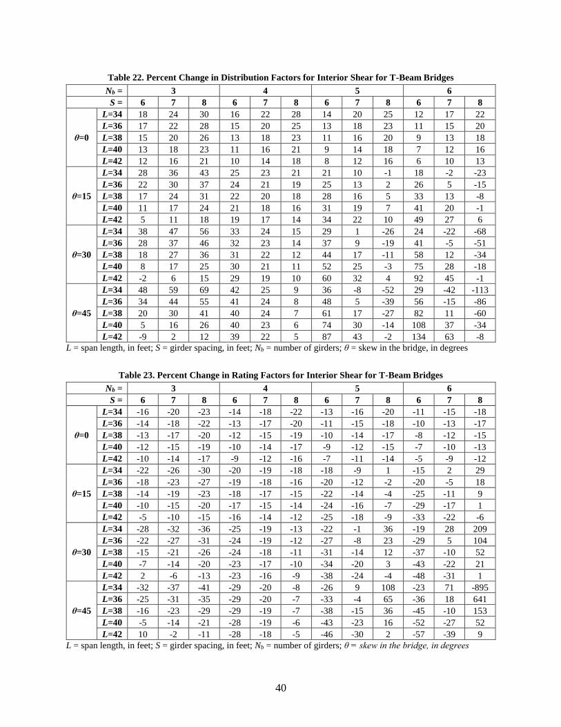
40

Table 22. Percent Change in Distribution Factors for Interior Shear for T-Beam Bridges

Nb = 3 4 5 6

S = 6 7 8 6 7 8 6 7 8 6 7 8

θ=0

L=34 18 24 30 16 22 28 14 20 25 12 17 22

L=36 17 22 28 15 20 25 13 18 23 11 15 20

L=38 15 20 26 13 18 23 11 16 20 9 13 18

L=40 13 18 23 11 16 21 9 14 18 7 12 16

L=42 12 16 21 10 14 18 8 12 16 6 10 13

θ=15

L=34 28 36 43 25 23 21 21 10 -1 18 -2 -23

L=36 22 30 37 24 21 19 25 13 2 26 5 -15

L=38 17 24 31 22 20 18 28 16 5 33 13 -8

L=40 11 17 24 21 18 16 31 19 7 41 20 -1

L=42 5 11 18 19 17 14 34 22 10 49 27 6

θ=30

L=34 38 47 56 33 24 15 29 1 -26 24 -22 -68

L=36 28 37 46 32 23 14 37 9 -19 41 -5 -51

L=38 18 27 36 31 22 12 44 17 -11 58 12 -34

L=40 8 17 25 30 21 11 52 25 -3 75 28 -18

L=42 -2 6 15 29 19 10 60 32 4 92 45 -1

θ=45

L=34 48 59 69 42 25 9 36 -8 -52 29 -42 -113

L=36 34 44 55 41 24 8 48 5 -39 56 -15 -86

L=38 20 30 41 40 24 7 61 17 -27 82 11 -60

L=40 5 16 26 40 23 6 74 30 -14 108 37 -34

L=42 -9 2 12 39 22 5 87 43 -2 134 63 -8

L = span length, in feet; S = girder spacing, in feet; Nb = number of girders; θ = skew in the bridge, in degrees

Table 23. Percent Change in Rating Factors for Interior Shear for T-Beam Bridges

Nb = 3 4 5 6

S = 6 7 8 6 7 8 6 7 8 6 7 8

θ=0

L=34 -16 -20 -23 -14 -18 -22 -13 -16 -20 -11 -15 -18

L=36 -14 -18 -22 -13 -17 -20 -11 -15 -18 -10 -13 -17

L=38 -13 -17 -20 -12 -15 -19 -10 -14 -17 -8 -12 -15

L=40 -12 -15 -19 -10 -14 -17 -9 -12 -15 -7 -10 -13

L=42 -10 -14 -17 -9 -12 -16 -7 -11 -14 -5 -9 -12

θ=15

L=34 -22 -26 -30 -20 -19 -18 -18 -9 1 -15 2 29

L=36 -18 -23 -27 -19 -18 -16 -20 -12 -2 -20 -5 18

L=38 -14 -19 -23 -18 -17 -15 -22 -14 -4 -25 -11 9

L=40 -10 -15 -20 -17 -15 -14 -24 -16 -7 -29 -17 1

L=42 -5 -10 -15 -16 -14 -12 -25 -18 -9 -33 -22 -6

θ=30

L=34 -28 -32 -36 -25 -19 -13 -22 -1 36 -19 28 209

L=36 -22 -27 -31 -24 -19 -12 -27 -8 23 -29 5 104

L=38 -15 -21 -26 -24 -18 -11 -31 -14 12 -37 -10 52

L=40 -7 -14 -20 -23 -17 -10 -34 -20 3 -43 -22 21

L=42 2 -6 -13 -23 -16 -9 -38 -24 -4 -48 -31 1

θ=45

L=34 -32 -37 -41 -29 -20 -8 -26 9 108 -23 71 -895

L=36 -25 -31 -35 -29 -20 -7 -33 -4 65 -36 18 641

L=38 -16 -23 -29 -29 -19 -7 -38 -15 36 -45 -10 153

L=40 -5 -14 -21 -28 -19 -6 -43 -23 16 -52 -27 52

L=42 10 -2 -11 -28 -18 -5 -46 -30 2 -57 -39 9

L = span length, in feet; S = girder spacing, in feet; Nb = number of girders; θ = skew in the bridge, in degrees

41

Observations from these results include:

Distribution factors mostly increased for bridges with characteristics that were within the

bounds presented in Table 22.

Increasing numbers of girders mostly leads to an increase in distribution factor.

Bridges with a high skew angle (30 or 45 degrees) and high girder spacing may have a

reduction in the distribution factor. The magnitude of this reduction increases with a

decrease in span length.

Exterior Shear. The regression model developed for exterior shear is shown in Equation

(14)Error! Reference source not found.. This four-parameter model had an R2 value of 0.8941

(89.41%). The primary parameters associated with this model were moment of inertia, slab

thickness, span length, and skew angle. Tables 24 and 25 illustrate the impacts across the

parameter space for both distribution factor and load rating factor. Observations from these

results include:

Distribution factors mostly increased for bridges with characteristics that were within the

bounds provided in Table 24.

As the skew angle increased, the percent increase in distribution factor mostly increased.

As the moment of inertia increased, the distribution factors tended to have a higher

probability of an increase.

ΔDFext-S = −580.9 + 17.08L + 73.81ts − 2.16L ∙ ts − 16.76×10-5

L ∙ I + 28.06×10-2

L ∙ θ

−77.74×10-2

ts ∙ θ + 2.216×10-5

L ∙ ts ∙ I − 1631×103L ∙ ts ∙ θ

−736.9×108L ∙ I ∙ θ + 4.026×10

-5ts ∙ I ∙ θ

(14)

Table 24. Percent Change in Distribution Factors for Exterior Shear for T-Beam Bridges

ts = 7 8 9

θ = 0 15 30 45 0 15 30 45 0 15 30 45

I=18000

L=34 -5 6 17 28 8 9 10 12 21 13 4 -4

L=36 -1 7 15 23 9 9 9 9 18 10 2 -6

L=38 3 8 14 19 9 8 7 5 15 7 0 -8

L=40 7 10 12 15 10 7 5 2 12 5 -3 -10

L=42 11 11 11 11 10 6 3 -1 9 2 -5 -12

I=24000

L=34 -9 12 32 52 8 18 29 39 25 25 26 26

L=36 -5 12 28 44 9 17 25 33 23 23 22 22

L=38 -1 12 24 36 10 16 21 27 21 20 19 17

L=40 3 11 20 28 11 14 17 21 19 17 15 13

L=42 7 11 16 20 12 13 14 14 17 14 11 8

I=30000

L=34 -12 17 47 77 8 28 47 67 28 38 48 57

L=36 -8 16 41 65 9 26 42 58 27 35 42 50

L=38 -5 15 34 53 11 23 36 48 26 32 37 43

L=40 -1 13 28 42 12 21 30 39 26 29 32 36

L=42 3 12 21 30 14 19 24 29 25 26 27 29

42

L = span length, in feet; S = girder spacing, in feet; I = girder moment of inertia, in inches4; θ = skew in the bridge,

in degrees

Table 252. Percent Change in Rating Factors for Exterior Shear for T-Beam Bridges

ts = 7 8 9

θ = 0 15 30 45 0 15 30 45 0 15 30 45

I=18000

L=34 6 -5 -14 -22 -7 -8 -9 -10 -18 -11 -4 4

L=36 1 -7 -13 -19 -8 -8 -8 -8 -15 -9 -2 7

L=38 -3 -8 -12 -16 -8 -7 -6 -5 -13 -7 0 9

L=40 -6 -9 -11 -13 -9 -7 -5 -2 -11 -5 3 11

L=42 -10 -10 -10 -10 -9 -6 -3 1 -8 -2 5 14

I=24000

L=34 10 -10 -24 -34 -7 -16 -22 -28 -20 -20 -21 -21

L=36 5 -10 -22 -31 -8 -15 -20 -25 -19 -18 -18 -18

L=38 1 -10 -19 -27 -9 -13 -18 -21 -17 -16 -16 -15

L=40 -3 -10 -17 -22 -10 -12 -15 -17 -16 -14 -13 -11

L=42 -6 -10 -14 -17 -11 -11 -12 -13 -14 -12 -10 -8

I=30000

L=34 14 -15 -32 -43 -7 -22 -32 -40 -22 -27 -32 -36

L=36 9 -14 -29 -39 -9 -20 -29 -37 -22 -26 -30 -33

L=38 5 -13 -25 -35 -10 -19 -26 -33 -21 -24 -27 -30

L=40 1 -12 -22 -29 -11 -17 -23 -28 -20 -22 -25 -26

L=42 -3 -11 -17 -23 -12 -16 -19 -23 -20 -21 -22 -22

L = span length, in feet; S = girder spacing, in feet; I = girder moment of inertia, in inches4; θ = skew in the bridge,

in degrees

Model Validation. The regression models were validated through a comparison of the

predictions to the results directly derived from the refined analyses of the selected set of bridges.

The change in the distribution factor for the moment and shear obtained from the refined analysis

(x-axis) versus the regression model (y-axis) for each T-beam bridge are shown in Figure

16Figure. The solid line in the plots indicates no difference between these two calculations. The

dashed lines in the plots represent the limits of 10% error between the regression model and the

refined analysis model. The results indicated that the prediction model developed herein can

make a reasonable estimate for the majority of the T-beam bridges used in this study for all load

effect cases. Similar to the steel girder bridge predictions, as the bridges approached or extended

beyond the parameter space, the models tended to lose accuracy, albeit with less extreme

differences than the steel girder bridges.

Slab Bridges

Recall that the load rating factor for a slab structure is directly proportional to the

effective width. The regression model developed for the slab bridge effective width is shown in

Equation (15). This four-parameter model had an R2 value of 0.9052 (90.52%). The primary

parameters associated with this model were span length, bridge width, skew angle, and parapet

width. Table 26 illustrates the impacts across the parameter space for effective width.

∆Ew = −289.4 + 23.09L + 10.07W + 57.88Pw + 10.73θ − 8.102×10-1

L ∙ W (15)

43

−14.94L ∙ Pw − 52.89L×10-2

L ∙ θ − 78.40×10-2

W ∙ Pw − 30.06×10-2

W ∙ θ

+ 41.26×10-2

Pw ∙ θ + 49.21×10-2

L ∙ W ∙ Pw + 14.71×10-3

L ∙ W ∙ θ

+ 13.97×10-2

L ∙ Pw ∙ θ − 11.93×10-2

W ∙ Pw ∙ θ

Figure 16. Percent Change in Distribution Factors for Reinforced Concrete T-Beam Bridges - Refined

Analysis Versus Regression Model: (a) interior moment; (b) exterior moment; (c) interior shear; (d)

exterior shear. Blue markers represent bridges within the parameter ranges of the regression model,

while red markers represent bridges outside that range together with corresponding bridge numbers in

Table 5.

Observations from these results include:

Effective width mostly increased for bridges with characteristics that were within the

defined bounds.

Bridges with small span lengths mostly had a higher possibility of an increase in effective

width.

44

An increase in bridge width mostly lead to an increase in effective width.

Bridges with larger parapet widths had a higher probability of an increase in effective

width.

Table 26. Percent Change in Effective Width for Slab Bridges

Pw = 1 1.12 1.25

W = 25 30 35 25 30 35 25 30 35

L=15

θ=0 4 26 49 3 30 57 3 34 65

θ=15 8 16 24 7 18 28 6 20 34

θ=30 13 6 -1 11 6 0 9 6 2

θ=45 18 -4 -26 15 -6 -28 12 -8 -29

L=20

θ=0 5 19 34 3 23 43 1 27 53

θ=15 8 13 18 6 16 26 5 19 34

θ=30 11 7 3 10 9 8 9 12 14

θ=45 14 1 -13 14 2 -9 13 4 -5

L=25

θ=0 6 12 19 2 16 29 -1 20 41

θ=15 7 10 13 6 14 23 4 19 34

θ=30 9 8 7 9 12 16 9 18 26

θ=45 10 5 0 12 11 9 14 17 19

L=30

θ=0 7 5 4 2 9 16 -4 13 29

θ=15 7 7 7 5 12 20 2 18 34

θ=30 7 9 10 8 16 24 9 23 38

θ=45 7 10 14 10 19 28 15 29 43

L = span length, in feet; W = slab width, in feet; Pw = parapet width, in feet; θ = skew in the bridge, in degrees

Model Validation. The predictions models developed were validated through a

comparison of the effective width results derived from the direct refined analyses. The change in

the effective width obtained from the refined analysis (x-axis) versus the regression model (y-

axis) for each slab bridge are shown in Figure 17. The solid line in the plot indicate no difference

45

Figure 17. Percent Change in Effective Width for Reinforced Concrete Slab Bridges - Refined Analysis

Versus Regression Model. Blue markers represent bridges within the regression model parameter ranges,

while red markers are for bridges outside that range together with corresponding bridge numbers in Table 6.

between these two parameters. The dashed lines represent the limits of 10% error between the

regression model and the refined analysis model. Note that in Table 26, the regression model

estimates for the percent change in the effective width are provided for the bridges with span

lengths of 25 ft, 30 ft, and 35 ft. In the results presented in Figure 17, there were a number of

bridges with a span length greater than 40 ft or less than 15 ft, i.e. outside the model boundaries.

Nevertheless, the regression model was able to make very close predictions for both bridges

within and outside of the model boundaries. In particular, the mean deviation between the

regression model estimate and refined analysis results for the change in the effective width was

2%.

CONCLUSIONS

The bridges in the VDOT inventory that are susceptible to load posting due to SHVs and EVs

primarily consist of steel girder-concrete deck, reinforced concrete T-beam, and slab bridges.

There are a large number of steel girder bridges with timber deck that are rated below one for

the SHVs; however, almost all of these bridges are located on secondary routes.

The plate with eccentric beam analysis (for girder bridges) and plate analysis (for slab

bridges) are more effective refined analysis methods in representing the load distribution

behavior when modeling with LARSA 4D. For the eccentric beam analysis, LARSA 4D allows

generating models automatically with little effort by using built-in templates that can also be

modified using spreadsheets. While the basic grid analysis approach can work for both of

these types of structures, using this method in LARSA 4D requires additional effort in placing

grid lines and calculating some sectional properties.

46

The moment distribution factors obtained from the refined analysis will likely result in

improved rating factors compared to those using distribution factors computed through the

AASHTO LRFD approach, as is the case for the shear distribution factors for exterior

girders.

The shear distribution factors for interior girders determined through refined analysis will

likely be greater than those calculated using the AASHTO LRFD approach. Consequently, the

rating factors for those bridges controlled by the shear capacity of interior beams will likely be

lower.

For the slab bridges, refined analysis tends to result in a higher effective slab width when

compared to the AASHTO LRFD approach. Single-lane loading conditions will likely have a

greater increase compared to multi-lane loaded cases.

RECOMMENDATIONS

1. VDOT’s Structure and Bridge Division should use the tables developed in this report as an

initial screening tool to identify bridge structures within their inventory that are vulnerable to

posting but have high potential for improvement in rating factors through the use of refined

analyses.

2. VDOT’s Structure and Bridge Division should employ a plate with eccentric beam approach

to model girder bridges and 2D plate analysis approach for slab bridges when conducting

refined analysis using LARSA 4D.

IMPLEMENTATION AND BENEFITS

Implementation

In regards to recommendation 1, VDOT’s Structure and Bridge Division will include the

tables developed within this report in the scope of the Load Rating Manual as a means for

VDOT’s load rating engineers to quickly identify potential candidate bridges that would benefit

from an improved load rating factor through refined analysis methods. The Load Rating Manual

is currently scheduled to be finished by September 30, 2021.

In regards to recommendation 2, VDOT’s Structure and Bridge Division will also include

in the scope of the Load Rating Manual a recommendation for the load rating engineer to use the

plate with eccentric beam analysis for girder bridges and plate analysis for slab bridges when

using refined analysis methods for the purposes of establishing more precise load distribution

behavior in its girder-concrete deck and slab bridges. The Load Rating Manual is currently

scheduled to be finished by September 30, 2021.

47

Benefits

With regards to recommendations 1 and 2, VDOT can continue to be in compliance with

federal mandates regarding the new SHV and EV load rating classifications. Beyond that,

however, many other bridges are on the cusp of posting requirements for the more traditional

load rating vehicles. At a time when VDOT must prioritize spending decisions for maintenance,

rehabilitation, and reconstruction, the tools generated from this research can help to alleviate the

pressure by offering more precision on the rating factors, resulting in a greater number of bridges

with a sufficient level of safety. This result will mitigate the number of unnecessarily posted

structures due to conservative calculations, and thus help to maintain the level of travel and

commerce across the Commonwealth.

ACKNOWLEDGEMENTS

The research team would like to acknowledge the support provided by VDOT in

execution of this research. This acknowledgement includes the TRP for providing guidance on

the project direction as well as the various districts.

REFERENCES

Adams, A., Galindez, N., Hopper, T., Murphy, T., Ritchie, P., Storlie, V., and Weisman, J.

(2019). Manual for Refined Analysis in Bridge Design and Evaluation (No. FHWA-HIF-

18-046). United States. Federal Highway Administration. Office of Infrastructure.

Amer, A., Arockiasamy, M. and Shahawy, M. (1999). Load distribution of existing solid slab

bridges based on field tests. Journal of Bridge Engineering, 4(3), pp.189-193.

American Association of State and Highway Transportation Officials (AASHTO) (2019).

Manual for Bridge Evaluation. 3rd Ed. with 2019 Interim Revisions. American

Association of State Highway and Transportation Officials, Washington, DC.

American Association of State Highway and Transportation Officials (AASHTO)

(2017). AASHTO LRFD Bridge Design Specifications. 8th Ed. American Association of

State Highway and Transportation Officials, Washington, DC.

Barker, M.G. (2001). Quantifying field-test behavior for rating steel girder bridges. Journal of

Bridge Engineering, 6(4), pp.254-261.

Catbas, F.N., Gokce, H.B. and Gul, M. (2012). Practical approach for estimating distribution

factor for load rating: Demonstration on reinforced concrete T-beam bridges. Journal of

Bridge Engineering, 17(4), pp.652-661.

Chiewanichakorn, M., Aref, A.J., Chen, S.S. and Ahn, I.S. (2004). Effective flange width

definition for steel–concrete composite bridge girder. Journal of Structural

Engineering, 130(12), pp.2016-2031.

48

Chung, W., Liu, J. and Sotelino, E.D. (2006). Influence of secondary elements and deck cracking

on the lateral load distribution of steel girder bridges. Journal of Bridge

Engineering, 11(2), pp.178-187.

Davids, W.G., Poulin, T.J. and Goslin, K. (2013). Finite-element analysis and load rating of flat

slab concrete bridges. Journal of Bridge Engineering, 18(10), pp.946-956.

Dymond, B.Z., French, C.E. and Shield, C.K. (2019). Recommendations for More Accurate

Shear Rating of Prestressed Concrete Girder Bridges. Journal of Bridge

Engineering, 24(12), p.04019117.

Eom, J. and Nowak, A.S. (2001). Live load distribution for steel girder bridges. Journal of

Bridge Engineering, 6(6), pp.489-497.

Federal Highway Administration (FHWA) (2013). Action: Load Rating of Specialized Hauling

Vehicles. Federal Highway Administration, McLean, VA.

Federal Highway Administration (FHWA) (2016). Fixing America’s surface transportation act

or ‘FAST Act’. Federal Highway Administration, McLean, VA.

Harris, D.K. (2010). Assessment of flexural lateral load distribution methodologies for stringer

bridges. Engineering Structures, 32(11), pp.3443-3451.

Harris, D.K., Ozbulut, O., Bagheri, A., Dizaji, M.S., Ndong, A.K. and Alipour, M. (2020). Load

Rating Strategies for Bridges With Limited or Missing As-Built Information (No.

FHWA/VTRC 20-R27). University of Virginia.

Hawkins, D.M. and Galpin, J.S. (1986). Selecting a Subset of Regression Variables so as to

Maximize the Prediction Accuracy at a Point. Journal of Applied Statistics, 13, pp.187-

199.

Islam, S. (2018). Load Rating Study of Effects of Special Hauling Vehicle Loads on Ohio

Bridges (Doctoral dissertation, University of Toledo).

Jáuregui, D.V., Licon-Lozano, A. and Kulkarni, K., 2007. Improved load rating of reinforced

concrete slab bridges (No. NM05STR-02). New Mexico. Dept. of Transportation.

Research Bureau.

Kim, S. and Nowak, A.S. (1997). Load distribution and impact factors for I-girder

bridges. Journal of Bridge Engineering, 2(3), pp.97-104.

LARSA, Inc. LARSA, Melville, NY.

Mabsout, M., Tarhini, K., Jabakhanji, R. and Awwad, E. (2004). Wheel load distribution in

simply supported concrete slab bridges. Journal of Bridge Engineering, 9(2), pp.147-155.

Mathworks, Inc. MATLAB, Natick, MA.

49

Nouri, G. and Ahmadi, Z. (2012). Influence of skew angle on continuous composite girder

bridge. Journal of Bridge Engineering, 17(4), pp.617-623.

Nowak, A.S. and Eom, J. (2001). Verification of Girder Distribution Factors and Dynamic Load

Factors by Field Testing. Current and future trends in bridge design, construction and

maintenance 2: Safety, economy, sustainability and aesthetics (pp. 414-423). Thomas

Telford Publishing.

R Core Team (2013). R: A language and environment for statistical computing. R Foundation for

Statistical Computing, Vienna, Austria

Sivakumar, B. (2007). NCHRP 12‐63: Legal truck loads and AASHTO legal loads for posting.

Report 575, National Cooperative Highway Research Board, Washington, D.C.

Snyder, R. and Beisswenger, J. (2017). Implementation of a Refined Shear Rating Methodology

for Prestressed Concrete Girder Bridges (No. MN/RC 2017-48). Minnesota. Dept. of

Transportation. Research Services & Library.

Virginia Department of Transportation (VDOT) (2019). State of the Structures and Bridges

Report. Virginia Department of Transportation, Richmond, VA.

Yousif, Z. and Hindi, R. (2007). AASHTO-LRFD live load distribution for beam-and-slab

bridges: Limitations and applicability. Journal of Bridge Engineering, 12(6), pp.765-773.

Zokaie, T., Imbsen, R. A., and Osterkamp, T. A. (1991). Distribution of Wheel Loads on

Highway Bridges, National Cooperative Highway Research Program (NCHRP 12-26).

Transportation Research Board, Washington, USA.