role of non-ideality for the ion transport in porous media
TRANSCRIPT
Role of non-ideality for the ion transport in porous media:
derivation of the macroscopic equations using upscaling
Gregoire Allairea,1,2, Robert Brizzia,2, Jean-Francois Dufrecheb,2, Andro Mikelicc,2,∗,Andrey Piatnitskid,2
a CMAP, Ecole Polytechnique, F-91128 Palaiseau, FrancebUniversite de Montpellier 2, Laboratoire Modelisation Mesoscopique et Chimie Theorique
(LMCT), Institut de Chimie Separative de Marcoule ICSM UMR 5257, CEA / CNRS / Universitede Montpellier 2 / ENSCM Centre de Marcoule, Bat. 426 BP 17171, 30207 Bagnols sur Ceze
Cedex, FrancecUniversite de Lyon, Lyon, F-69003, France; Universite Lyon 1, Institut Camille Jordan, UMR
5208, Bat. Braconnier, 43, Bd du 11 novembre 1918, 69622 Villeurbanne Cedex, Franced Narvik University College, Postbox 385, Narvik 8505, Norway; Lebedev Physical Institute,
Leninski prospect 53, 119991, Moscow, Russia
Abstract
This paper is devoted to the homogenization (or upscaling) of a system of partialdifferential equations describing the non-ideal transport of a N-component electrolytein a dilute Newtonian solvent through a rigid porous medium. Realistic non-idealeffects are taken into account by an approach based on the mean spherical approxi-mation (MSA) model which takes into account finite size ions and screening effects.We first consider equilibrium solutions in the absence of external forces. In such acase, the velocity and diffusive fluxes vanish and the equilibrium electrostatic poten-tial is the solution of a variant of Poisson-Boltzmann equation coupled with algebraicequations. Contrary to the ideal case, this nonlinear equation has no monotone struc-
∗Corresponding authorEmail addresses: [email protected] (Gregoire Allaire),
[email protected] (Robert Brizzi), [email protected](Jean-Francois Dufreche), [email protected] (Andro Mikelic), [email protected](Andrey Piatnitski)
1G. A. is a member of the DEFI project at INRIA Saclay Ile-de-France.2This research was partially supported by the project DYMHOM (De la dynamique moleculaire,
via l’homogeneisation, aux modeles macroscopiques de poroelasticite et electrocinetique) from theprogram NEEDS (Projet federateur Milieux Poreux MIPOR), GdR MOMAS and GdR PARIS. Theauthors would like to thank O. Bernard, V. Marry, P. Turq and B. Rotenberg from the laboratoryPhysicochimie des Electrolytes, Colloides et Sciences Analytiques (PECSA), UMR CNRS 7195,Universit P. et M. Curie, for helpful discussions.
Preprint submitted to Elsevier June 8, 2014

ture. However, based on invariant region estimates for Poisson-Boltzmann equationand for small characteristic value of the solute packing fraction, we prove existenceof at least one solution. To our knowledge this existence result is new at this levelof generality. When the motion is governed by a small static electric field and asmall hydrodynamic force, we generalize O’Brien’s argument to deduce a linearizedmodel. Our second main result is the rigorous homogenization of these linearizedequations and the proof that the effective tensor satisfies Onsager properties, namelyis symmetric positive definite. We eventually make numerical comparisons with theideal case. Our numerical results show that the MSA model confirms qualitativelythe conclusions obtained using the ideal model but there are quantitative differencesarising that can be important at high charge or high concentrations.
Keywords: Modified Boltzmann-Poisson equation, MSA, homogenization,electro-osmosisPACS: 02.30.Jr, 47.61.Fg, 47.56.+r, 47.57.J-, 47.70.Fw, 47.90.+a, 82.70.Dd,91.60.Pn
1. Introduction
The quasi-static transport of an electrolyte through an electrically charged porousmedium is an important and well-known multiscale problem in geosciences and porousmaterials modeling. An N -component electrolyte is a dilute solution of N species ofcharged particles, or ions, in a fluid which saturates a rigid charged porous medium[36]. The macroscopic dynamics of such a system is controlled by several phenomena.First the global hydrodynamic flow, which is commonly modelled by the Darcy’s lawdepends on the geometry of the pores and also on the charge distributions of thesystem. Second, the migration of ions because of an electric field can be quantifiedby the conductivity of the system. Third, the diffusion motion of the ions is modifiedby the interaction with the surfaces, but also by the interactions between the soluteparticles. Lastly, electrokinetic phenomena are due to the electric double layer(EDL) which is formed as a result of the interaction of the electrolyte solution whichneutralizes the charge of the solid phase at the pore solid-liquid interface. Thus, anexternal electric field can generate a so-called electro-osmotic flow and reciprocally,when a global hydrodynamic flow is applied, an induced streaming potential is createdin the system.
The EDL can be split into several parts, depending on the strength of the elec-trostatic coupling. There is a condensed layer of ions of typical size lG for whichthe attraction energy with the surface eΣ/E lG (with Σ the surface charge and ethe elementary charge) is much more than the thermal energy kBT (with kB Boltz-mann’s constant and T the temperature). The corresponding characteristic length
2

lG = EkBT/Σe (Gouy length) is typically less than one nanometer. Consequently,the layer of heavily adsorbed ions practically depends on the molecular nature ofthe interface and it is generally known as the Stern layer. After the Stern layerthe electrostatic diffuse layer or Debye’s layer is formed, where the ion densityvaries. The EDL is the union of Stern and diffuse layers. The thickness of the diffuselayer is predicted by the Debye length λD which depends on the electrolyte concentra-tion. For low to moderate electrolyte concentrations λD is in the nanometric range.Outside Debye’s layer, in the remaining bulk fluid, the solvent can be considered aselectrically neutral.
The large majority of theoretical works are concerned with a simple (so-calledideal) model for which the departure of ideality of ions are neglected (see later inthis introduction a precise definition of ideality). Thus the macroscopic descriptionsof charged porous media such as the ones using finite element methods [1], homoge-nization approaches [39] or lattice-Boltzmann methods [51] are commonly based onthe Poisson-Nernst-Planck formalism for which the local activity coefficients of ionsare neglected and the transport properties are modelled solely from the mobility atinfinite dilution. In addition, the boundary condition for the electrostatic interactionbetween the two phases is very often simplified by replacing the bare surface chargeΣ, which corresponds to the chemistry of the system, by surface potential Ψ. Itsboundary value at the no slip plane is known as the zeta potential ζ. In fact, it israther the surface charge density Σ, proportional to the normal derivative of Ψ, thanζ, which is the relevant parameter (this is confirmed by an asymptotic analysis in[7]).
A few studies do not model the details of the EDL. Under the presence of anexternal electric field E, the charged fluid may acquire a plug electro-osmotic flowvelocity which is proportional to Eζ and given by the so-called Smoluchowski’s for-mula. In the case of porous media with large pores, the electro-osmotic effects aremodeled by introducing an effective slip velocity at the solid-liquid interfaces, whichcomes from the Smoluchowski formula. In this setting, the effective behavior of thecharge transport through spatially periodic porous media was studied by Edwardsin [22], using the volume averaging method. These methods for which the transportbeyond the EDL is uncoupled from the one in the EDL are not valid for numeroussystems, such as clays because the characteristic pore size is also of the order of theEDL size (a few hundreds of nanometers or even less). Therefore the Debye’s layerfills largely the pores and its effect cannot anymore be modeled by an effective slipboundary condition at the liquid-solid interface.
In the present paper, we consider continuum equations (such as the Navier-Stokesor the Fick equations) as the right model for the description of porous media at thepore scale where the EDL phenomena and the pore geometry interact. The typical
3

length scale for which these continuous approach are valid is confirmed to be bothexperimentally (see e.g. [13]) and theoretically [38, 16] close to 1 nanometer. There-fore, we consider continuum equations at the microscopic level and, more precisely,we couple the incompressible Stokes equations for the fluid with the electrokineticmodel made of a global electrostatic equation and one convection-diffusion equationfor each type of ions.
The most original ingredient of the model is the treatment of the departure fromideality. Electrolyte solutions are not ideal anymore as fas as the ion concentration isnot dilute [9]. Typically simple 1-1 electrolyte, such as NaCl in water have an activitycoefficient which is close to 0.6 at molar concentrations (while it is equal to 1 bydefinition in the ideal case) and the non ideality effects is even more important for thetransport coefficients [19, 15]. Thus any ideal model can only be in semi-quantitativeagreement with a more rigorous model if departure from ideality are neglected. In thepresent article, we use a new approach based on the Mean Spherical Approximation(MSA), for which the ions are considered to be charged hard spheres [27, 12]. Thismodel is able to describe the properties of the solutions up to molar concentrations.In addition, a generalization of the Fuoss-Onsager theory based on the Smoluchowskiequation has been developped [21, 11, 19, 18, 20, 15] by taking into account thismodel, and it is possible to predict the various transport coefficients of bulk electrolytesolutions up to molar concentrations. This MSA transport equations extend the wellknown Debye-Huckel-Onsager limiting law to the domain of concentrated solutions.They have also been proved to be valid [29] for confined solutions in the case of claysby comparing their predictions to molecular and Brownian dynamics simulations.
A more detailed, mathematically oriented, presentation of the fundamental con-cepts of electroosmotic flow in nanochannels can be found in the book [31] by Karni-adakis et al., pages 447-470, from which we borrow the notations and definitions inthis introduction. We now describe precisely our stationary model, describing at thepore scale the electro-chemical interactions of an N -component electrolyte in a diluteNewtonian solvent. All quantities are given in SI units. We start with the followingmass conservation laws
div
(ji + uni
)= 0 in Ωp, i = 1, . . . , N, (1)
where Ωp is the pore space of the porous medium Ω, i denotes the solute species, u isthe hydrodynamic velocity and ni is the ith species concentration. For each speciesi, uni is its convective flux and ji its migration-diffusion flux.
The solute velocity is given by the incompressible Stokes equations with a forcingterm made of an exterior hydrodynamical force f and of the electric force applied to
4

the fluid thanks to the charged species
η∆u = f +∇p+ e
N∑j=1
zjnj∇Ψ in Ωp, (2)
div u = 0 in Ωp, (3)
u = 0 on ∂Ωp \ ∂Ω, (4)
where η > 0 is the shear viscosity, p is the pressure, e is the elementary charge, zi isthe charge number of the species i and Ψ is the electrostatic potential. The pore spaceboundary is ∂Ωp while ∂Ω is the outer boundary of the porous medium Ω. On thefluid/solid boundaries ∂Ωp \ ∂Ω we assume the no-slip boundary condition (4). Forsimplicity, we shall assume that Ω is a rectangular domain with periodic boundaryconditions on ∂Ω. Furthermore, in order to perform a homogenization process, weassume that the pore distribution is periodic in Ωp.
We assume that all valencies zj are different. If not, we lump together different ionswith the same valency. Of course, for physical reasons, all valencies zj are integers.We rank them by increasing order and we assume that they are both anions andcations, namely positive and negative valencies,
z1 < z2 < ... < zN , z1 < 0 < zN , (5)
and we denote by j+ and j− the sets of positive and negative valencies.The migration-diffusion flux ji is given by the following linear relationship
ji = −N∑j=1
Lij(n1, . . . , nN)(∇µj + zje∇Ψ
), i = 1, . . . , N, (6)
where Lij(n1, . . . , nN) is the Onsager coefficient between i and j and µj is the chemicalpotential of the species j given by
µj = µ0j + kBT lnnj + kBT ln γj(n1, . . . , nN), j = 1, . . . , N, (7)
with γj being the activity coefficient of the species j, kB is the Boltzmann constant,µ0j is the standard chemical potential expressed at infinite dilution and T is the
absolute temperature. The sum of all fluxes ji is not zero because the solvent isnot considered here and ji is a particle flux. The Onsager tensor Lij is made of thelinear Onsager coefficients between the species i and j. It is symmetric and positivedefinite. Furthermore, on the fluid/solid interfaces a no-flux condition holds true
ji · ν = 0 ∂Ωp \ ∂Ω, i = 1, . . . , N. (8)
5

The electrostatic potential is calculated from Poisson equation with the electric chargedensity as bulk source term
E∆Ψ = −eN∑j=1
zjnj in Ωp, (9)
where E = E0Er is the dielectric constant of the solvent. The surface charge Σ isassumed to be given at the pores boundaries, namely the boundary condition reads
E∇Ψ · ν = −Σ on ∂Ωp \ ∂Ω, (10)
where ν is the unit exterior normal to Ωp.The activity coefficients γi and the Onsager coefficients Lij depend on the elec-
trolyte. At infinite dilution the solution can be considered ideal and we have γi = 1and Lij = δijniD
0i /(kBT ), where D
0i > 0 is the diffusion coefficient of species i at
infinite dilution. At finite concentration, these expressions which correspond to thePoisson-Nernst-Planck equations are not valid anymore. Non-ideal effects modifythe ion transport and they are to be taken into account if quantitative descriptionof the system is required. Different models can be used. Here we choose the MeanSpherical Approximation (MSA) in simplified form [19] which is valid if thediameters of the ions are not too different. The activity coefficients read
ln γj = −LBΓz
2j
1 + Γσj+ ln γHS, j = 1, . . . , N, (11)
where σj is the j-th ion diameter, LB is the Bjerrum length given by LB = e2/(4πEkBT ),γHS is the hard sphere term defined by (13), and Γ is the MSA screening param-eter defined by
Γ2 = πLB
N∑k=1
nkz2k
(1 + Γσk)2. (12)
For dilute solutions, i.e., when all nj are small, we have
2Γ ≈ κ =1
λDwith λD =
√EkBT
e2∑N
k=1 nkz2k,
where λD is the Debye length. Thus, 1/2Γ generalizes λD at finite concentration andit represents the size of the ionic spheres when the ion diameters σi are different fromzero. (In the sequel we shall use a slightly different definition of the Debye length,
6

relying on the notion of characteristic concentration, see Table 1.) In (11) γHS is thehard sphere term which is independent of the type of species and is given by
ln γHS = p(ξ) ≡ ξ8− 9ξ + 3ξ2
(1− ξ)3, with ξ =
π
6
N∑k=1
nkσ3k, (13)
where ξ is the solute packing fraction.The Onsager coefficients Lij are given by
Lij(n1, . . . , nN) = ni
(D0
i
kBTδij +Ωij
)(1 +Rij
), i, j = 1, . . . , N, (14)
where Ωij = Ωcij + ΩHS
ij stands for the hydrodynamic interactions in the MSA for-malism and there is no summation for repeated indices in (14). It is divided into twoterms: the Coulombic part is
Ωcij = − 1
3η
zizjLBnj
(1 + Γσi)(1 + Γσj)
(Γ +
N∑k=1
nkπLBz
2kσk
(1 + Γσk)2
) , (15)
and the hard sphere part is
ΩHSij = −(σi + σj)
2
12ηnj
1− X3/5 + (X3)2/10
1 + 2X3
, (16)
with
X3 =π
6
N∑i=1
ni3X1X2 +X3X0
4X20
and Xk =π
6
N∑i=1
niσki . (17)
In (14) Rij is the electrostatic relaxation term given by
Rij =κ2qe
2zizj
3EkBT (σi + σj)(1 + Γσi)(1 + Γσj)
1− e−2κq(σi+σj)
κ2q + 2Γκq + 2Γ2 − 2πLB
N∑k=1
nkz2ke
−κqσk
(1 + Γσk)2
(18)
where κq > 0 is defined by
κ2q =e2
EkBT
∑Ni=1 niz
2iD
0i∑N
i=1D0i
. (19)
7

All these coefficients γj,Γ,Ωij,Rij are varying in space since they are functions of theconcentrations nj. The N ×N tensor (Lij) is easily seen to be symmetric. However,to be coined ”Onsager tensor” it should be positive too, which is not obvious from theabove formulas. The reason is that they are only approximations for not too largeconcentrations. Nevertheless, when the concentrations nj are small, all entries Lij
are first order perturbations of the ideal values δijniD0i /(kBT ) and thus the Onsager
tensor is positive at first order. The various parameters appearing in (1)-(19) aredefined in Table 1.
QUANTITY CHARACTERISTIC VALUEe electron charge 1.6e−19 C (Coulomb)D0
i diffusivity of the ith species D0i ∈ (1.333, 2.032)e−09m2/s
kB Boltzmann constant 1.38e−23 J/Knc characteristic concentration (6.02 1024, 6.02 1026) particles/m3
T temperature 293K (Kelvin)E dielectric constant 6.93e−10C/(mV )η dynamic viscosity 1e−3 kg/(ms)ℓ pore size 5e−9 m
λD Debye’s length√EkBT/(e2nc) ∈ (0.042, 0.42) nm
zj j-th electrolyte valence given integerΣ surface charge density 0.129C/m2 (clays)f given applied force N/m3
σj j-th hard sphere diameter 2e−10 mΨc characteristic electrokinetic potential 0.02527 V (Volt)LB Bjerrum length 7.3e−10 m
Table 1: Data description
As already said we consider a rectangular domain Ω =∏d
k=1(0, Lk)d (d = 2, 3 is
the space dimension), Lk > 0 and at the outer boundary ∂Ω we set
Ψ + Ψext(x) , ni , u and p are Ω− periodic. (20)
The applied exterior potential Ψext(x) can typically be linear, equal to E · x, whereE is an imposed electrical field. Note that the applied exterior force f in the Stokesequations (2) can also be interpreted as some imposed pressure drop or gravity force.Due to the complexity of the geometry and of the equations, it is necessary for engi-neering applications to upscale the system (1)-(10) and to replace the flow equationswith a Darcy type law, including electro-osmotic effects.
8

It is a common practice to assume that the porous medium has a periodic mi-crostructure. For such media, and in the ideal case, formal two-scale asymptoticanalysis of system (1)-(10) has been performed in many previous papers. Many ofthese works rely on a preliminary linearization of the problem which is first due toO’Brien et al. [45]. Let us mention in particular the work of Looker and Carnie in[35] that we rigorously justify in [5] and for which we provided numerical experimentsin [6]. Other relevant references include [1], [2], [8], [14], [26], [37], [39], [40], [41], [42],[43], [50], [47], [48], [53].
Our goal here is to generalize these works for the non-ideal MSA model. Morespecifically, we extend our previous works [5], [6] and provide the homogenized systemfor a linearized version of (1)-(10) in a rigid periodic porous medium (the linearizationis performed around a so-called equilibrium solution which satisfies the full nonlinearsystem (1)-(10) with vanishing fluxes). The homogenized system is an elliptic systemof (N + 1) equations
−divxM∇(p0, µj1≤j≤N) = S in Ω,
where p0 is the pressure, µj the chemical potential of the j-th species, M the On-sager homogenized tensor and S a source term. The (N + 1) equations express theconservation of mass for the fluid and the N species. More details will be given inSection 5.
In Section 2 we provide a dimensionless version of system (1)-(10). We also explainin Lemma 1 how the ideal case can be recovered from the non-ideal MSA model in thelimit of small characteristic value of the solute packing fraction. Section 3 is concernedwith the definition of so-called equilibrium solutions when the external forces arevanishing (but not the surface charge Σ). Computing these equilibrium solutionsamounts to solve a MSA variant of the nonlinear Poisson-Boltzmann equation for thepotential. Existence of a solution to such a Poisson-Boltzmann equation is establishedin Section 6 under a smallness assumption for a characteristic value of the solutepacking fraction. To our knowledge this existence result is the first one at this level ofgenerality. Let us mention nevertheless that, in a slightly simpler setting (two speciesonly and a linear approximation of p(ξ)) and with a different method (based on asaddle point approach in the two variables Ψ and nj), a previous existence resultwas obtained in [24]. In Section 4 we give a linearized version of system (1)-(10). Wegeneralize the seminal work of O’Brien et al. [45], which was devoted to the ideal case,to the present setting of the MSA model. Under the assumption that all ions have thesame diameter σj we establish in Proposition 11 and Lemma 12 that the linearizedmodel is well-posed and that its solution satisfies uniform a priori estimates. Thisproperty is crucial for homogenization of the linearized model which is performedin Section 5. Following our work [5] in the ideal case, we rigorously obtained the
9

homogenized problem in Theorem 14 and derive precise formulas for the effectivetensor in Proposition 15. Furthermore we prove that the so called Onsager relation(see e.g. [25]) is satisfied, namely the full homogenized tensorM is symmetric positivedefinite.
Eventually Section 7 is devoted to a numerical study of the obtained homoge-nized coefficients, including their sensitivities to various physical parameters and asystematic comparison with the ideal case.
2. Non-dimensional form
Before studying its homogenization, we need a dimensionless form of the equa-tions (1)-(10). We follow the same approach as in our previous works [5], [6]. Theknown data are the characteristic pore size ℓ, the characteristic domain size L, thesurface charge density Σ (having the characteristic value Σc), the static electrical po-tential Ψext and the applied fluid force f . As usual, we introduce a small parameterε which is the ratio between the pore size and the medium size, ε = ℓ/L << 1.
We are interested in characteristic concentrations nc taking on typical values inthe range (10−2, 1) in Mole/liter, that is (6.02 1024, 6.02 1026) particles per m3. FromTable 1, we write λD =
√EkBT/(e2nc) and we find out that λD varies in the range
(0.042, 0.42) nm.Following [31], we introduce the characteristic potential ζ = kBT/e and the pa-
rameter β related to the Debye-Huckel parameter κ = 1/λD, as follows
β =
(ℓ
λD
)2
. (21)
Next we rescale the space variable by setting x′ = x/L and Ω′ = Ω/L =∏d
k=1(0, L′k)
d
(we shall drop the primes for simplicity in the sequel). The rescaled dimensions L′k
are assumed to be independent of ε. Similarly, the pore space becomes Ωε = Ωp/Lwhich is a periodically perforated domain with period ε. Still following [31], wedefine other characteristic quantities
Γc =√πLBnc, pc = nckBT, uc = ε2
kBTncL
η,
where Γc, in terms of nc, is deduced from (12), pc is a pressure equilibrating theelectrokinetic forces in (2) and uc is the velocity corresponding to a Poiseuille flow in atube of diameter ℓ, length L and pressure drop pc. We also introduce adimensionalizedforcing terms
Ψext,∗ =eΨext
kBT, f∗ =
fL
pc, Σ∗ =
Σ
Σc
, Nσ =eΣcℓ
EkBT,
10

and adimensionalized unknowns
Γε =Γ
Γc
, pε =p
pc, uε =
u
uc, Ψε =
eΨ
kBT, nε
j =nj
nc
, jεj =jjL
ncD0j
.
The dimensionless equations for hydrodynamical and electrostatic part are thus
ε2∆uε −∇pε = f∗ +N∑j=1
zjnεj(x)∇Ψε in Ωε, (22)
uε = 0 on ∂Ωε \ ∂Ω, div uε = 0 in Ωε, (23)
−ε2∆Ψε = β
N∑j=1
zjnεj(x) in Ωε; (24)
ε∇Ψε · ν = −NσΣ∗ on ∂Ωε \ ∂Ω, (25)
(Ψε +Ψext,∗), uε and pε are Ω− periodic in x. (26)
(Recall that Ω =∏d
k=1(0, Lk)d so that periodic boundary conditions make sense for
such a rectangular domain.) Furthermore, from (11) and (12) we define
γεj = γHSε exp−
LBΓεΓcz
2j
(1 + ΓεΓcσj) and (Γε)2 =
N∑k=1
nεkz
2k
(1 + ΓcΓεσk)2. (27)
The solute packing fraction ξ is already an adimensionalized quantity (taking valuesin the range (0, 1)). However, introducing a characteristic value ξc we can adimen-sionalize its formula (13) as
ξc =π
6ncσ
3c , ξ = ξc
N∑k=1
nεk(σkσc
)3, (28)
where σc is the characteristic ion diameter. We note that Γc ∈ (0.117, 1.17) 109 m−1,Γcσc ∈ (0.023, 0.23), LBΓc ∈ (0.0857, 0.857) and ξc ∈ (0.252, 25.2) 10−4 which is asmall parameter. Concerning Ωc
ij which has to be compared with D0i /(kBT ), we find
out that
LBnckBT/(3ηΓcD0i ) = ΓckBT/(3πηD
0i ) ∈ (0.005415, 0.5415),
while ΩHSij is slightly smaller andRij looks negligible. Concerning the transport term,
the Peclet number for the j-th species is
Pej =ucL
D0j
=ℓ2kBTnc
ηD0j
∈ (0.01085, 1.085).
11

After these considerations we obtain the dimensionless form of equation (1):
div
(jεi + Pein
εiu
ε
)= 0 in Ωε, i = 1, . . . , N, (29)
jεi · ν = 0 on ∂Ωε \ ∂Ω, i = 1, . . . , N, (30)
jεi = −N∑j=1
nεiK
εij∇M ε
j and M εj = ln
(nεjγ
εj e
zjΨε), (31)
Kεij =
(δij +
kBT
D0i
Ωij
)(1 +Rij
), i, j = 1, . . . , N. (32)
Eventually the porous medium Ωε is assumed to be an ε-periodic smooth opensubset of Ω =
∏dk=1(0, Lk)
d and Lk/ε are integers for every k and every ε. It is builtfrom Ω by removing a periodic distributions of solid obstacles which, after rescalingby 1/ε, are all similar to the unit obstacle YS. More precisely, we consider a smoothpartition of the unit periodicity cell Y = YS ∪YF where YS is the solid part and YF isthe fluid part. The liquid/solid interface is S = ∂YS \ ∂Y . The fluid part is assumedto be a smooth connected open subset (no assumption is made on the solid part). Wedefine Y j
ε = ε(YF + j) and Ωε =∪
j∈Zd
Y jε ∩ Ω.
We also assume a periodic distribution of charges Σ∗ ≡ Σ∗(x/ε). This will implythat, at equilibrium (in the absence of other forces), the solution of system (22)-(32)is also periodic of period ε.
We recall that the ideal model (see e.g. [31]) corresponds to the following valuesof the activity coefficient, γi = 1, and of the Onsager tensor Lij = δijniD
0i /(kBT ).
In view of our previous dimensional analysis it is interesting to see in which sensethe present non-ideal MSA model is close to the ideal case. We shall make thisconnection in the limit of a small parameter going to zero. More precisely we relyon the characteristic value ξc of the solute packing fraction, defined by (28). Thesmallness of ξc (which means a low concentration, weighted by the ion size) willbe a crucial assumption in Theorem 2 that establishes the existence of equilibriumsolutions to the MSA model. It is therefore a natural parameter to study the limitideal case. With this goal in mind we introduce two additional dimensionless numbers:the Bjerrum’s parameter (also called the Landau plasma parameter)
bi =LB
σc, (33)
and the ratio appearing in Stokes’ formula for the drag hydrodynamic force
S =kBT
ηD0cσc
, (34)
12

where D0c is the characteristic value for the diffusivities D0
i , 1 ≤ i ≤ N . According tothe numerical values of Table 1, we assume that
bi and S are of order one. (35)
More precisely, it is enough to assume that bi and S are bounded quantities when ξcbecomes infinitely small (they can tend to zero too).
Lemma 1. Under assumption (35), the ideal case is the limit of our non-ideal MSAmodel for small solute packing fraction ξc, namely
Kεij = δij +O(
√ξc), and ln γεj = O(
√ξc). (36)
Hence the MSA model is a regular O(√ξc) perturbation of the idealized model.
Theorem 2 in Section 3 gives the equilibrium MSA solution as an O(√ξc) perturba-
tion of the equilibrium idealized solution. The arguments from Section 6 could beextended to interpret the MSA variant of Poisson-Boltzmann equation as an O(
√ξc)
perturbation of the classical (ideal) Poisson-Boltzmann equation.
Proof. In view of formula (13) we find
ln γHS = O(ξc).
From its definition (12) and for small ξc we deduce that
Γ = O(√LBnc).
Using assumption (35), bi = O(1), yields
Γσj = O(√biξc) = O(
√ξc) and ΓLB = O(
√bi3ξc) = O(
√ξc),
which implies from (11)
−LBΓz
2j
1 + Γσj= O(
√ξc) and thus ln γj = O(
√ξc).
Turning to the Onsager coefficients, we obtain from (19) that
κqσc = O(√LBncσc) = O(
√ξc),
which implies after some algebra that
Rij = O(LBκq) = O(√ξc).
13
Using the second part of assumption (35), S = O(1), yields
Ωcij
kBT
D0i
= O(kBT
ηD0cσc
√biξc) = O(S
√biξc) = O(
√ξc).
Similarly
ΩHSij
kBT
D0i
= O(Sξc) = O(ξc),
which eventually yields
Lij =niD
0i
kBT(δij +O(
√ξc)),
from which we infer the conclusion (36). Note that a similar approximation holds forthe chemical potential
µj = µ0j + kBT (lnnj +O(
√ξc)).
3. Equilibrium solution
The goal of this section is to find a so-called equilibrium solution of system(22)-(32) when the exterior forces are vanishing f = 0 and Ψext = 0. However, thesurface charge density Σ∗ is not assumed to vanish or to be small. This equilibriumsolution will be a reference solution around which we shall linearize system (22)-(32)in the next section. Then we perform the homogenization of the (partially) linearizedsystem. We denote by n0,ε
i ,Ψ0,ε,u0,ε,M0,εi , p0,ε the equilibrium quantities.
In the case f = 0 and Ψext = 0, one can find an equilibrium solution by choosinga zero fluid velocity and taking all diffusion fluxes equal to zero. More precisely, werequire
u0,ε = 0 and ∇M0,εj = 0, (37)
which obviously implies that j0,εi = 0 and (29)-(30) are satisfied. The Stokes equation(22) shall give the corresponding value of the pressure satisfying
∇p0,ε(x) = −N∑j=1
zjn0,εj (x)∇Ψ0,ε(x),
for which an explicit expression is given below (see (47)). From ∇M0,εj = 0 and (31)
we deduce that there exist constants n0j(∞) > 0 and γ0j (∞) > 0 such that
n0,εj (x) = n0
j(∞)γ0j (∞)exp−zjΨ0,ε(x)
γ0,εj (x). (38)
14

The value n0j(∞) is the reservoir concentration (also called the infinite dilute con-
centration) which will be later assumed to satisfy the bulk electroneutrality condi-tion for zero potential. The value γ0j (∞) is the reservoir activity coefficient which
corresponds to the value of γ0,εj for zero potential (see (49) below for its precise for-mula). Before plugging (38) into Poisson equation (24) to obtain the MSA variant ofPoisson-Boltzmann equation for the potential Ψ0,ε, we have to determine the value ofthe activity coefficient γ0,εj .
From the first equation of (27) we have
γ0,εj = γHS(ξ) exp−LBΓ
0,εΓcz2j
1 + Γ0,εΓcσj = expp(ξ)−
LBΓ0,εΓcz
2j
1 + Γ0,εΓcσj, (39)
where, for ξ ∈ [0, 1), p(ξ) is a polynomial defined by (13) and, recalling definition(28) of the characteristic value ξc, the solute packing fraction ξ is
ξ = ξc
N∑j=1
n0,εj (
σjσc
)3. (40)
The second equation of (27) gives a formula for the MSA screening parameter
(Γ0,ε)2 =N∑k=1
n0,εk z2k
(1 + ΓcΓ0,εσk)2. (41)
Let us explain how to solve the algebraic equations (38), (39), (40) and (41).Combining (38), (39) and (40), for given potential Ψ0,ε and screening parameter
Γ0,ε, the solute packing fraction ξ is a solution of the algebraic equation
ξ = exp−p(ξ)ξcN∑j=1
(σjσc
)3n0j(∞)γ0j (∞) exp
−zjΨ0,ε +
LBΓ0,εΓcz
2j
1 + Γ0,εΓcσj
. (42)
Once we know ξ ≡ ξ(Ψ0,ε,Γ0,ε), solution of (42), combining (38) and (41), Γ0,ε is asolution of the following algebraic equation, depending on Ψ0,ε,
(Γ0,ε)2 =N∑j=1
n0j(∞)γ0j (∞)
z2j(1 + Γ0,εΓcσj)2
exp
−zjΨ0,ε +
LBΓ0,εΓcz
2j
1 + Γ0,εΓcσj− p
(ξ(Ψ0,ε,Γ0,ε)
).
(43)
All in all, solving the two algebraic equations (42) and (43) yields the values Γ0,ε(Ψ0,ε)
and ξ(Ψ0,ε) ≡ ξ(Ψ0,ε,Γ0,ε(Ψ0,ε)
)(see Section 6 for a precise statement).
15

Then the electrostatic equation (24) reduces to the following MSA variant ofPoisson-Boltzmann equation which is a nonlinear partial differential equation for thesole unknown Ψ0,ε −ε2∆Ψ0,ε = β
N∑j=1
zjn0j(∞)γ0j (∞) exp
−zjΨ0,ε +
LBΓ0,ε(Ψ0,ε)Γcz
2j
1 + Γ0,ε(Ψ0,ε)Γcσj− p(ξ(Ψ0,ε))
in Ωε,
ε∇Ψ0,ε · ν = −NσΣ∗ on ∂Ωε \ ∂Ω, Ψ0,ε is Ω− periodic.
(44)In Section 6 (see Theorem 24) we shall prove the following existence result. Un-
fortunately we are unable to prove uniqueness.
Theorem 2. Assuming that the surface charge distribution Σ∗ belongs to L∞(∂Ωε),that the ions are not too small, namely
LB < (6 + 4√2) min
1≤j≤N
σjz2j
with 6 + 4√2 ≈ 11.656854, (45)
and that the characteristic value ξc is small enough, there exists at least one solutionof (44) Ψ0,ε ∈ H1(Ωε) ∩ L∞(Ωε).
Introducing the primitive Ej(Ψ) of
E ′j(Ψ) = zjn
0j(∞)γ0j (∞) exp−zjΨ+
LBΓ0,ε(Ψ)Γcz
2j
1 + Γ0,ε(Ψ)Γcσj− p(ξ(Ψ)), (46)
the equilibrium pressure in Stokes equations (corresponding to a zero velocity) isgiven (up to an additive constant) by
p0,ε =N∑j=1
Ej(Ψ0,ε). (47)
Remark 3. In the ideal case, i.e., when γ0,εj = 1, the function Ej(Ψ0,ε) defined by
(46) is simply equal to n0,εj = n0
j(∞) exp−zjΨ0,ε.
From a physical point of view, it is desired that the solution of (44) vanishes, i.e.,Ψ0,ε = 0, when the surface charges are null, i.e., Σ∗ = 0. Therefore, following theliterature, we impose the bulk electroneutrality condition
N∑j=1
E ′j(0) = −
N∑j=1
zjn0j(∞)γ0j (∞) exp
LBΓ0,ε(0)Γcz
2j
1 + Γ0,ε(0)Γcσj− p(ξ(0)) = 0, (48)
16

where Γ0,ε(0) is the solution of (43) for Ψ0,ε = 0.Defining the equilibrium activity coefficient by
γ0j (∞) = expp(ξ(0))−LBΓ
0,ε(0)Γcz2j
1 + Γ0,ε(0)Γcσj, (49)
the bulk electroneutrality condition (48) reduces to its usual form
N∑j=1
zjn0j(∞) = 0.
Formula (49) is an implicit algebraic equation for γ0j (∞) since ξ(0) and Γ0,ε(0) dependthemselves on the γ0k(∞)’s. The next Lemma proves that it is a well-posed equation.
Lemma 4. There always exists a unique solution γ0j (∞) of the algebraic equation(49).
Proof. Assume that there exists γ0j (∞) satisfying (49) and plug this formula in (43).It yields (
Γ0,ε(0))2
=N∑j=1
n0j(∞)z2j
(1 + Γ0,ε(0)Γcσj)2,
which admits a unique solution Γ0,ε(0) > 0 since the left hand side is strictly increasingand the right hand side is decreasing. On the same token, using (49) in (42) leads to
ξ(0) = ξc
N∑j=1
(σjσc
)3n0j(∞).
We have thus found explicit values for Γ0,ε(0) and ξ(0) which do not depend on theγ0k(∞)’s. Using them in (49) gives its unique solution γ0j (∞).
Remark 5. From the proof of Lemma 4 it is clear that Γ0,ε(0) does not depend onξc, while ξ(0) = O(ξc), which implies that γ0j (∞) = O(1) for small ξc.
Remark 6. The bulk electroneutrality condition (48) is not a restriction. Actuallyall our results hold under the much weaker assumption (5) that all valencies zj do nothave the same sign. Indeed, if (48) is not satisfied, we can make a change of variablesin the Poisson-Boltzmann equation (44), defining a new potential Ψ0,ε = Ψ0,ε + Cwhere C is a constant reference potential. Since the function
C → Φ(C) =N∑j=1
zjn0j(∞)γ0j (∞) exp−zjC +
LBΓ0,ε(C)Γcz
2j
1 + Γ0,ε(C)Γcσj− p(ξ(C))
17

is continuous and admits opposite infinite limits when C tends to ±, there exists atleast one value C such that Φ(C) = 0. This change of variables for the potential leaves(43) and (44) invariant if we change the constants n0
j(∞)γ0j (∞) in new constants
n0j(∞)γ0j (∞) = n0
j(∞)γ0j (∞) exp−zjC+LBΓ
0,ε(C)Γcz2j
1 + Γ0,ε(C)Γcσj−LBΓ
0,ε(0)Γcz2j
1 + Γ0,ε(0)Γcσj−p(ξ(C))+p(ξ(0)).
These new constants satisfy the bulk electroneutrality condition (48).
4. Linearization
We now proceed to the linearization of electrokinetic equations (22-32) around theequilibrium solution computed in Section 3. We therefore assume that the externalforces, namely the static electric potential Ψext(x) and the hydrodynamic force f(x),are small. However, the surface charge density Σ∗ on the pore walls is not assumedto be small since it is part of the equilibrium problem studied in Section 3. Sucha linearization process is classical in the ideal case (see the seminal paper [45] byO’Brien et al.) but it is new and slightly more complicated for the MSA model. Forsmall exterior forces, we write the perturbed electrokinetic unknowns as
nεi (x) = n0,ε
i (x) + δnεi (x), Ψε(x) = Ψ0,ε(x) + δΨε(x),
uε(x) = u0,ε(x) + δuε(x), pε(x) = p0,ε(x) + δpε(x),
where n0,εi ,Ψ0,ε,u0,ε, p0,ε are the equilibrium quantities, corresponding to f = 0 and
Ψext = 0. The δ prefix indicates a perturbation. Since the equilibrium velocityvanishes u0,ε = 0, we identify in the sequel uε = δuε.
Motivated by the form of the Boltzmann equilibrium distribution and the calcu-lation of n0,ε
i , we follow the lead of [45] and introduce a so-called ionic potential Φεi
which is defined in terms of nεi by
nεi (x)γ
εi (x) = n0
i (∞)γ0j (∞) exp−zi(Ψε(x) + Φεi (x) + Ψext,∗(x)), (50)
where
γεi = expp(ξ)− LBΓεΓcz
2i
1 + ΓεΓcσi and (Γε)2 =
N∑k=1
nεkz
2k
(1 + ΓεΓcσk)2, (51)
with
p(ξ) = ξ8− 9ξ + 3ξ2
(1− ξ)3and ξ = ξc
N∑j=1
nεj(σjσc
)3.
Since Φ0,εi = 0 by virtue of formula (38) for n0,ε
i , we identify δΦεi with Φε
i .
18

Lemma 7. The linearization of (50-51) yields
δnεi (x) =
N∑k=1
zkα0,εi,k (x)
(δΨε(x) + Φε
k(x) + Ψext,∗(x)), (52)
with
α0,εi,k = −n0,ε
i δik +B0,εn0,εi n0,ε
k σ3k −
LBΓc
A0,εn0,εi n0,ε
k (53)
×(
z2i(1 + Γ0,εΓcσi)2
−B0,εC0,ε
)(z2k
(1 + Γ0,εΓcσk)2−B0,εD0,εσ3
k
),
where
B0,ε =π6ncp
′(ξ)
1 + ξp′(ξ), C0,ε =
N∑k=1
z2kσ3kn
0,εk
(1 + Γ0,εΓcσk)2, D0,ε =
N∑k=1
z2kn0,εk
(1 + Γ0,εΓcσk)2
and
A0,ε = 2Γ0,ε + 2Γc
N∑k=1
n0,εk z2kσk
(1 + Γ0,εΓcσk)3− LBΓc
N∑k=1
n0,εk z4k
(1 + Γ0,εΓcσk)4
+LBΓcB0,εC0,ε
N∑k=1
n0,εk z2k
(1 + Γ0,εΓcσk)2.
Under assumption (45) of Theorem 2 the coefficient A0,ε is positive.Furthermore, at equilibrium, if we consider n0,ε
i as a function of Ψ0,ε, we have
dn0,εi
dΨ0,ε=
N∑k=1
zkα0,εi,k . (54)
If all ions have the same diameter (σk = σi for all i, k), then the coefficients α0,εi,k = α0,ε
k,i
are symmetric.
Remark 8. At equilibrium, the concentrations n0,εi , as well as the screening parameter
Γ0,ε, depend only on Ψ0,ε through the algebraic equations (38), (39), (40) and (41).However, outside equilibrium the concentrations nε
i and the screening parameter Γε
depend through (50-51) on the entire family (δΨε + Φεk +Ψext,∗), 1 ≤ k ≤ N .
19

Proof. Linearizing (50) leads to
δnεi =
−δγεi(γ0,εi )2
n0i (∞)γ0j (∞) exp−ziΨ0,ε−
zin0i (∞)γ0j (∞)
γ0,εi
exp−ziΨ0,ε(δΨε+Φε
i+Ψext,∗)
which is equivalent to
δnεi =
−δγεiγ0,εi
n0,εi − zin
0,εi
(δΨε + Φε
i +Ψext,∗). (55)
Linearization of the first equation of (51) yields
δγεiγ0,εi
= p′(ξ)δξ − LBΓcz2i
(1 + Γ0,εΓcσi)2δΓε with δξ =
π
6nc
N∑k=1
σ3kδn
εk. (56)
Multiplying (55) by σ3i and (56) by σ3
i n0,εi , then summing up to eliminate δγεi /γ
0,εi ,
gives(N∑k=1
σ3kδn
εk
)(1 +
π
6ncp
′(ξ)N∑k=1
σ3kn
0,εk
)= −
N∑k=1
σ3kzkn
0,εk
(δΨε+Φε
k+Ψext,∗)+δΓε
N∑k=1
LBΓcz2kσ
3kn
0,εk
(1 + Γ0,εΓcσk)2,
from which, together with (55), we deduce
δnεi (x) = −zin0,ε
i (x)(δΨε(x) + Φε
i (x) + Ψext,∗(x))+
LBΓcz2i n
0,εi (x)
(1 + Γ0,ε(x)Γcσi)2δΓε(x) (57)
+B0,εn0,εi (x)
N∑k=1
σ3kzkn
0,εk (x)
(δΨε(x) + Φε
k(x) + Ψext,∗(x))−B0,εC0,εn0,ε
i (x)LBΓcδΓε(x).
Next, we linearize the second formula of (51) to obtain
2Γ0,εδΓε =N∑k=1
(z2kδn
εk
(1 + Γ0,εΓcσk)2− 2n0,ε
k z2kσkΓc
(1 + Γ0,εΓcσk)3δΓε
).
Combining it with (57) leads to
A0,ε(x) δΓε(x) = −N∑k=1
n0,εk (x)z3k
(1 + Γ0,ε(x)Γcσk)2
(δΨε(x) + Φε
k(x) + Ψext,∗(x))
(58)
+B0,ε(x)D0,ε(x)N∑k=1
n0,εk (x)zkσ
3k
(δΨε(x) + Φε
k(x) + Ψext,∗(x)).
20

Eventually, plugging (58) into (57) yields (52) and (53).Since we divide by A0,ε we check that it does not vanish in some range of the phys-
ical parameters. Using definition (51) of (Γ0,ε)2 in the equality 2Γ0,ε = 2(Γ0,ε)2/Γ0,ε
allows us to rewrite the coefficient A0,ε as
A0,ε(x) = Γc
N∑k=1
n0,εk z2k
(1 + Γ0,εΓcσk)2
(2
Γ0,εΓc
+2σk
(1 + Γ0,εΓcσk)− LBz
2k
(1 + Γ0,εΓcσk)2
)
+LBΓcB0,εC0,ε
N∑k=1
n0,εk z2k
(1 + Γ0,εΓcσk)2,
where each term in the sum of the first line is positive under the same condition (45)and same proof as in Lemma 18.
The computation leading to (54) is completely similar. Finally, the symmetryrelation α0,ε
i,k = α0,εk,i is obvious from formula (53) when σk = σi for all i, k.
Remark 9. In the ideal case, γεi ≡ 1, Lemma 7 simplifies a lot since α0,εi,k = −n0,ε
i δikwhich implies there is no coupling between the various ionic potentials in the definitionof a single species concentration.
Thanks to the definition (50) of the ionic potential, the linearization of the convection-diffusion equation (29) is easy because the diffusive flux simplifies as
M εj = ln
(nεjγ
εj e
zjΨε)
= ln(n0j(∞)γ0j (∞)
)− zj(Φ
εj +Ψext,∗).
Furthermore, the equilibrium solution satisfies ∇M0,εj = 0, which implies
div
( N∑j=1
n0,εi K0,ε
ij zj∇(Φεj +Ψext,∗) + Pein
0,εi uε
)= 0 in Ωε (59)
K0,εij =
(D0
i
kBTδij + Ω0
ij
)(1 +R0
ij
), i, j = 1, . . . , N. (60)
The linearization of the Stokes equation (22) is more tricky. We first get
ε2∆uε −∇δpε = f∗ +N∑j=1
zj(δnε
j∇Ψ0,ε + n0,εj ∇δΨε
)in Ωε, (61)
divuε = 0 in Ωε, uε = 0 on ∂Ωε \ ∂Ω.
We rewrite the sum on the right hand side of (61) as
∇
(N∑j=1
zjn0,εj δΨε
)+ Sε with Sε =
N∑j=1
zj(δnε
j∇Ψ0,ε − δΨε∇n0,εj
). (62)
21

Since ∇n0,εj =
dn0,εj
dΨ0,ε∇Ψ0,ε at equilibrium, from Lemma 7 we deduce
Sε =N∑
j,k=1
zj
(zkα
0,εj,k
(δΨε + Φε
k +Ψext,∗)− zkα
0,εj,kδΨ
ε)∇Ψ0,ε
=N∑
j,k=1
zjzkα0,εj,k
(Φε
k +Ψext,∗)∇Ψ0,ε (63)
If all ions have the same diameter, the coefficients α0,εj,k are symmetric, i.e. α0,ε
j,k = α0,εk,j,
so we deduce
Sε =N∑k=1
zkdn0,ε
k
dΨ0,ε
(Φε
k +Ψext,∗)∇Ψ0,ε =
N∑k=1
zk
(Φε
k +Ψext,∗)∇n0,ε
k .
Thus, we rewrite (61) as
ε2∆uε −∇P ε = f∗ −N∑j=1
zjn0,εj ∇
(Φε
j +Ψext,∗) , (64)
where the new pressure P ε is defined by
P ε = δpε +N∑j=1
zjn0,εj
(δΨε + Φε
j +Ψext,∗) .Remark 10. When the ion diameters are different, we can merely introduce nonlinearfunctions Fj (defined by their derivatives) such that
Sε =N∑j=1
zj(Φε
j +Ψext,∗)∇(Fj(Ψ0,ε)).
In general it is not clear whether Fj = nj.
Of course, one can deduce a linearized equation for δΨε from the non-linear Pois-son equation (24) too. But, since δΨε does not enter the previous equations (uponredefining the pressure P ε), it is decoupled from the main unknowns uε, P ε and Φε
i .Therefore it is not necessary to write its equation in details.
To summarize, we have just proved the following result.
22
Proposition 11. Assume that all ions have the same diameter. The linearized sys-tem, around the equilibrium solution of Section 3, of the electrokinetic equations (22-32) is
ε2∆uε −∇P ε = f∗ −N∑j=1
zjn0,εj ∇
(Φε
j +Ψext,∗) in Ωε, (65)
divuε = 0 in Ωε, uε = 0 on ∂Ωε \ ∂Ω, (66)
div n0,εi
( N∑j=1
K0,εij zj∇(Φε
j +Ψext,∗) + Peiuε
)= 0 in Ωε, i = 1, . . . , N, (67)
N∑j=1
K0,εij zj∇(Φε
j +Ψext,∗) · ν = 0 on ∂Ωε \ ∂Ω, (68)
uε, P ε, Φεj are Ω− periodic, (69)
where the coefficients n0,εj and K0,ε
ij (defined by (60)) are evaluated at equilibrium.
This is the system of equations that we are going to homogenize in the next sec-tions. It is the extension to the non-ideal case of a similar ideal system previouslystudied in [5], [6], [1], [2], [14], [26], [37], [50], [35]. The mathematical structure ofsystem (65)-(69) is essentially the same as in the ideal case. The only difference isthe coupling of the diffusion equations through the tensor K0,ε
ij . Note that the tensor
K0,εij is related to the original Onsager tensor Lij, defined in (14): upon adimension-
alization and evaluation at equilibrium, Lij becomes L0,εij = n0,ε
i K0,εij D
0i /(kBT ). In
particular, the tensor L0,εij inherits from the symmetry of Lij (it is thus symmetric
positive definite).Next, we establish the variational formulation of (65)-(69) and prove that it admits
a unique solution. The functional spaces related to the velocity field are
W ε = v ∈ H1(Ωε)d, v = 0 on ∂Ωε \ ∂Ω, Ω− periodic in x
andHε = v ∈ W ε, div v = 0 in Ωε.
The variational formulation of (65)-(69) is: find uε ∈ Hε and Φεjj=1,...,N ∈ H1(Ωε)N ,
Φεj being Ω-periodic, such that, for any test functions v ∈ Hε and ϕjj=1,...,N ∈
H1(Ωε)N , ϕj being Ω-periodic,
a((uε, Φε
j), (v, ϕj))= ⟨L, (v, ϕj)⟩,
23

where the bilinear form a and the linear form L are defined by
a((uε, Φε
j), (v, ϕj)):= ε2
∫Ωε
∇uε : ∇v dx+N∑
i,j=1
zizjPei
∫Ωε
n0,εi K0,ε
ij ∇Φεj · ∇ϕi dx
+N∑j=1
zj
∫Ωε
n0,εj
(uε · ∇ϕj − v · ∇Φε
j
)dx
⟨L, (v, ϕj)⟩ :=N∑j=1
zj
∫Ωε
n0,εj E∗ · v dx−
N∑i,j=1
zizjPei
∫Ωε
n0,εi K0,ε
ij E∗ · ∇ϕi dx−∫Ωε
f∗ · v dx,
(70)
where, for simplicity, we denote by E∗ the electric field corresponding to the potentialΨext,∗, i.e., E∗(x) = ∇Ψext,∗(x).
Lemma 12. For sufficiently small values of nc > 0 and ξc > 0, and under assumption(45), there exists a unique solution of (65)-(69), uε ∈ Hε and Φε
jj=1,...,N ∈ H1(Ωε)N ,Φε
j being Ω-periodic. Furthermore, there exists a positive constant C, independent ofε, such that
∥uε∥L2(Ωε)d + ε∥∇uε∥L2(Ωε)d2 + max1≤j≤N
∥Φεj∥H1(Ωε) ≤ C
(∥E∗∥L2(Ω)d + ∥f∗∥L2(Ω)d
).
(71)
Proof. Assumption (45) and ξc > 0 small implies that the potential Ψ0,ε is boundedin L∞(Ωε) (see Theorem 24). The same holds true for ξ and Γ0,ε which are alge-braic functions of Ψ0,ε. Thus, the concentrations n0,ε
j , defined by (109) are uniformlypositive and bounded in L∞(Ωε). Due to the structure of Ωc
ij, ΩHSij and Rij, these
coefficients, evaluated at equilibrium, are arbitrary small in L∞(Ωε) for small nc. Con-sequently, the tensor K0,ε
ij is positive definite (as a perturbation of the identity) andthe bilinear form a is coercive for nc ≤ ncr
c . The rest of the proof, including the a prioriestimates, is similar to the ideal case, studied in [5], where we had K0,ε
ij = δij.
5. Homogenization
In the previous sections 3 and 4 we did not use our assumption that the porousmedium and the surface charge distribution are ε-periodic (see the end of section2). Our further analysis relies crucially on this ε-periodicity hypothesis. Theorem2 gives the existence of a solution to the Poisson-Boltzmann equation (44) but not
24
its uniqueness. Nevertheless, we can define a particular solution of (44), which isε-periodic,
Ψ0,ε(x) = Ψ0(x
ε), (72)
where Ψ0(y) is a solution of the unit cell Poisson-Boltzmann equation
−∆yΨ0(y) = β
N∑j=1
zjn0j(y) in YF ,
∇yΨ0 · ν = −NσΣ
∗(y) on ∂YF \ ∂Y,y → Ψ0(y) is 1− periodic,
n0j(y) = n0
j(∞)γ0j (∞)exp −zjΨ0(y)
γ0j (y),
(73)
with the activity coefficient defined by
γ0j (y) = γHS(y) exp−LBΓ
0(y)Γcz2j
(1 + Γ0(y)Γcσj) and (Γ0(y))2 =
N∑k=1
n0k(y)z
2k
(1 + ΓcΓ0(y)σk)2,
and
γHS = expp(ξ) with p(ξ) = ξ8− 9ξ + 3ξ2
(1− ξ)3and ξ(y) =
πnc
6
N∑k=1
n0k(y)σ
3k.
The formal two-scale asymptotic expansion method [10], [28], [52] can be appliedto system (65)-(69) as in the ideal case studied by [35], [39], [40], [41], [43], [5] and[6]. Introducing the fast variable y = x/ε, it assumes that the solution of (65)-(69) isgiven by
uε(x) = u0(x, x/ε) + εu1(x, x/ε) + . . . ,P ε(x) = p0(x) + εp1(x, x/ε) + . . . ,Φε
j(x) = Φ0j(x) + εΦ1
j(x, x/ε) + . . . .(74)
We then plug this ansatz in the equations (65)-(69) and use the chain-rule lemmafor a function ϕ(x, x
ε)
∇(ϕ(x,
x
ε))=
(∇xϕ+
1
ε∇yϕ
)(x,
x
ε).
Identifying the various powers of ε we obtain a cascade of equations from which weretain only the first ones that constitute the following two-scale homogenized problem.This type of calculation is classical and we do not reproduce it here. It can be maderigorous thanks to the notion of two-scale convergence [3], [44].
25

Proposition 13. From each bounded sequence wε in L2(Ωε) one can extract asubsequence which two-scale converges to a limit w ∈ L2(Ω× YF ) in the sense that
limε→0
∫Ωε
wε(x)φ(x,x
ε
)dx =
∫Ω
∫YF
w(x, y)φ(x, y) dy dx
for any φ ∈ L2(Ω;Cper(Y )
)(“per” denotes 1-periodicity).
For sequences of functions wε defined in the perforated domain Ωε and satisfyinguniform in ε H1-bounds, it is well-known [28] that one can build extensions to theentire domain Ω satisfying the same uniform bounds. We implicitly assume suchextensions in the theorem below but do not give details which are classical and maybe found in [5].
Theorem 14. Under the assumptions of Lemma 12 the solution of (65)-(69) con-verges in the following sense
uε → u0(x, y) in the two-scale sense
ε∇uε → ∇yu0(x, y) in the two-scale sense
P ε → p0(x) strongly in L2(Ω)
Φεj → Φ0
j(x) weakly in H1(Ω) and strongly in L2(Ω)
∇Φεj → ∇xΦ
0j(x) +∇yΦ
1j(x, y) in the two-scale sense
where (u0, p0) ∈ L2(Ω;H1per(Y )d)×L2
0(Ω) and Φ0j ,Φ
1jj=1,...,N ∈
(H1(Ω)× L2(Ω;H1
per(Y )))N
is the unique solution of the two-scale homogenized problem
−∆yu0(x, y) +∇yp
1(x, y) = −∇xp0(x)− f∗(x)
+N∑j=1
zjn0j(y)
(∇xΦ
0j(x) +∇yΦ
1j(x, y) + E∗(x)
)in Ω× YF , (75)
divyu0(x, y) = 0 in Ω× YF , u0(x, y) = 0 on Ω× S, (76)
26

divx
(∫YF
u0(x, y) dy
)= 0 in Ω, (77)
−divyn0i (y)
( N∑j=1
Kij(y)zj(∇yΦ
1j(x, y) +∇xΦ
0j(x) + E∗(x)
)+ Peiu
0(x, y)
)= 0 in Ω× YF ,
(78)
N∑j=1
Kij(y)zj(∇yΦ
1j +∇xΦ
0j + E∗) · ν(y) = 0 on Ω× S, (79)
−divx
∫YF
n0i (y)
( N∑j=1
Kij(y)zj(∇yΦ
1j(x, y) +∇xΦ
0j(x) + E∗(x)
)+ Peiu
0(x, y)
)dy = 0 in Ω,
(80)
Φ0i ,
∫YF
u0 dy and p0 being Ω-periodic in x, (81)
with periodic boundary conditions on the unit cell YF for all functions depending ony and S = ∂YS \ ∂Y .
The limit problem introduced in Theorem 14 is called the two-scale and two-pressure homogenized problem, following the terminology of [28], [32]. It features twoincompressibility constraints (76) and (77) which are exactly dual to the two pressuresp0(x) and p1(x, y) which are their corresponding Lagrange multipliers. Remark thatequations (75), (76) and (78) are just the leading order terms in the ansatz of theoriginal equations. On the other hand, equations (77) and (80) are averages on theunit cell YF of the next order terms in the ansatz. For example, (77) is deduced from
divyu1(x, y) + divxu
0(x, y) = 0 in Ω× YF
by averaging on YF , recalling that u1(x, y) = 0 on Ω× S.
Proof. The proof of convergence and the derivation of the homogenized system iscompletely similar to the proof of Theorem 1 in [5] which holds in the ideal case.The only point which deserves to be made precise here is the well-posedness of thetwo-scale homogenized problem.
Following section 3.1.2 in [4], we introduce the functional space for the velocities
V = u0(x, y) ∈ L2per
(Ω;H1
per(YF )d)
satisfying (76)− (77),
which is known to be orthogonal in L2per
(Ω;H1
per(YF )d)to the space of gradients of the
form ∇xq(x)+∇yq1(x, y) with q(x) ∈ H1per(Ω)/R and q1(x, y) ∈ L2
per
(Ω;L2
per(YF )/R).
27

We define the functional space X = V ×H1per(Ω)/R× L2
per(Ω;H1per(YF )
d/R) and thevariational formulation of (75)-(81) is to find (u0, Φ0
j ,Φ1j) ∈ X such that, for any
test functions (v, ϕ0j , ϕ
1j) ∈ X,
a((u0, Φ0
j ,Φ1j), (v, ϕ0
j , ϕ1j))= ⟨L, (v, ϕ0
j , ϕ1j)⟩, (82)
where the bilinear form a and the linear form L are defined by
a((u0, Φ0
j ,Φ1j), (v, ϕ0
j , ϕ1j)):=
∫Ω
∫YF
∇yu0 : ∇v dx dy
+N∑
i,j=1
zizjPei
∫Ω
∫YF
n0iKij(∇xΦ
0j +∇yΦ
1j) · (∇xϕ
0j +∇yϕ
1j) dx dy (83)
+N∑j=1
zj
∫Ω
∫YF
n0j
(u0 · (∇xϕ
0j +∇yϕ
1j)− v · (∇xΦ
0j +∇yΦ
1j))dx dy
and
< L, (v, ϕj) >:=N∑j=1
zj
∫Ω
∫YF
n0jE
∗ · v dx dy −∫Ω
∫YF
f∗ · v dx dy
−N∑
i,j=1
zizjPei
∫Ω
∫YF
n0iKijE
∗ · (∇xϕ0j +∇yϕ
1j) dx dy,
We apply the Lax-Milgram lemma to prove the existence and uniqueness of the solu-tion in X of (82). The only point which requires to be checked is the coercivity of thebilinear form. We take v = u0, ϕ0
j = Φ0j and ϕ1
j = Φ1j as the test functions in (82).
We define a local diffusion tensor
K(y) =
(zizjPei
Kij(y)n0i (y)
)1≤i,j≤N
=
(kBT
ucLzizjLij(y)
)1≤i,j≤N
, (84)
which is symmetric since (Lij) is symmetric too. As already remarked in the proof ofLemma 12, K is uniformly coercive for small enough nc > 0 and ξc > 0. Therefore,the second integral on the right hand side of (83) is positive. The third integral, beingskew-symmetric, vanishes, which proves the coercivity of a.
Of course, one should extract from (75)-(81) the macroscopic homogenized prob-lem, which requires to separate the fast and slow scale. In the ideal case, Looker andCarnie in [35] proposed a first approach which was further improved in [5] and [6].
28

The main idea is to recognize in the two-scale homogenized problem (75)-(81) thatthere are two different macroscopic fluxes, namely (∇xp
0(x)+ f∗(x)) and ∇xΦ0j(x)+
E∗(x)1≤j≤N . Therefore we introduce two family of cell problems, indexed by k ∈1, ..., d for each component of these fluxes. We denote by ek1≤k≤d the canonicalbasis of Rd.
The first cell problem, corresponding to the macroscopic pressure gradient, is
−∆yv0,k(y) +∇yπ
0,k(y) = ek +N∑j=1
zjn0j(y)∇yθ
0,kj (y) in YF (85)
divyv0,k(y) = 0 in YF , v0,k(y) = 0 on S, (86)
−divyn0i (y)
( N∑j=1
Kij(y)zj∇yθ0,kj (y) + Peiv
0,k(y)
)= 0 in YF (87)
N∑j=1
Kij(y)zj∇yθ0,kj (y) · ν = 0 on S. (88)
The second cell problem, corresponding to the macroscopic diffusive flux, is for eachspecies l ∈ 1, ..., N
−∆yvl,k(y) +∇yπ
l,k(y) =N∑j=1
zjn0j(y)(δlje
k +∇yθl,kj (y)) in YF (89)
divyvl,k(y) = 0 in YF , vl,k(y) = 0 on S, (90)
−divyn0i (y)
( N∑j=1
Kij(y)zj(δlje
k +∇yθl,kj (y)
)+ Peiv
l,k(y)
)= 0 in YF (91)
N∑j=1
Kij(y)zj(δlje
k +∇yθl,kj (y)
)· ν = 0 on S, (92)
where δij is the Kronecker symbol. As usual the cell problems are complemented withperiodic boundary conditions.
29

Then, we can decompose the solution of (75)-(81) as
u0(x, y) =d∑
k=1
(−v0,k(y)
(∂p0
∂xk+ f ∗
k
)(x) +
N∑i=1
vi,k(y)
(E∗
k +∂Φ0
i
∂xk
)(x)
)(93)
p1(x, y) =d∑
k=1
(−π0,k(y)
(∂p0
∂xk+ f ∗
k
)(x) +
N∑i=1
πi,k(y)
(E∗
k +∂Φ0
i
∂xk
)(x)
)(94)
Φ1j(x, y) =
d∑k=1
(−θ0,kj (y)
(∂p0
∂xk+ f ∗
k
)(x) +
N∑i=1
θi,kj (y)
(E∗
k +∂Φ0
i
∂xk
)(x)
). (95)
We average (93)-(95) in order to get a purely macroscopic homogenized problem. Wedefine the homogenized quantities: first, the electrochemical potential
µj(x) = −zj(Φ0j(x) + Ψext,∗(x)), (96)
then, the ionic flux of the jth species
jj(x) =1
|YF |
∫YF
n0j(y)
( N∑l=1
Kjl(y)zlPej
(∇yΦ
1l (x, y)+∇xΦ
0l (x)+E∗(x)
)+u0
)dy, (97)
and finally the filtration velocity
u(x) =1
|YF |
∫YF
u0(x, y) dy. (98)
From (93)-(95) we deduce the homogenized or upscaled equations for the above ef-fective fields.
Proposition 15. Introducing the flux J (x) = (u, jj1≤j≤N) and the gradient F(x) =(∇xp
0, ∇xµj1≤j≤N), the macroscopic equations are
divxJ = 0 in Ω, (99)
J = −MF −M(f∗, 0), (100)
with a homogenized tensor M defined by
M =
KJ1z1
. . .JNzN
L1D11
z1· · · D1N
zN...
.... . .
...
LNDN1
z1· · · DNN
zN
, (101)
30

and complemented with periodic boundary conditions for p0 and Φ0j1≤j≤N . The
matrices Ji, K, Dji and Lj are defined by their entries
Jilk =1
|YF |
∫YF
vi,k(y) · el dy,
Klk =1
|YF |
∫YF
v0,k(y) · el dy,
Djilk =1
|YF |
∫YF
n0j(y)
(vi,k(y) +
N∑m=1
Kjm(y)zmPej
(δime
k +∇yθi,km (y)
) )· el dy,
Ljlk =1
|YF |
∫YF
n0j(y)
(v0,k(y) +
N∑m=1
Kjm(y)zmPej
∇yθ0,km (y)
)· el dy.
Furthermore, M is symmetric positive definite, which implies that the homogenizedequations (99)-(100) have a unique solution.
Remark 16. The symmetry of M is equivalent to the famous Onsager’s reciprocalrelations. In the ideal case, the symmetry of the tensor M was proved in [35], [5].
Proof. The conservation law (99) is just a rewriting of (77) and (80). The constitutiveequation (100) is an immediate consequence of the definitions (97) and (98) of thehomogenized fluxes, taking into account the decomposition (93)-(95).
We now prove thatM is positive definite. For any collection of vectors λ0, λi1≤i≤N ∈Rd let us introduce the following linear combinations of the cell solutions
vλ =d∑
k=1
(λ0kv
0,k +N∑i=1
λikvi,k
), θλj =
d∑k=1
(λ0kθ
0,kj +
N∑i=1
λikθi,kj
), (102)
which satisfy
−∆yvλ(y) +∇yπ
λ(y) = λ0 +N∑j=1
zjn0j(y)
(λj +∇yθ
λj (y)
)in YF (103)
divyvλ(y) = 0 in YF , vλ(y) = 0 on S, (104)
−divy
(n0i (y)
(N∑j=1
zjKij(λj +∇yθ
λj (y)) + Peiv
λ(y)
))= 0 in YF (105)
N∑j=1
zjKij(λj +∇yθ
λj (y)) · ν = 0 on S, (106)
31

Multiplying the Stokes equation (103) by vλ, the convection-diffusion equation (105)by θλj and summing up, we obtain∫
YF
(|∇yv
λ(y)|2 +N∑
i,j=1
zizjPei
n0i (y)Kij(y)(∇yθ
λj (y) + λj) · (∇yθ
λi (y) + λi)
)dy
=
∫YF
λ0 · vλ dy +N∑i=1
∫YF
zin0iλ
i · vλ dy +N∑
i,j=1
∫YF
zizjPei
n0iKij(∇yθ
λj + λj) · λi dy
= Kλ0 · λ0 +N∑i=1
Jiλi · λ0 +N∑
i,j=1
ziλi · Dijλ
j +N∑i=1
ziλi · Liλ
0 = M(λ0, ziλi)T · (λ0, ziλi)T .
The left hand side of the above equality is positive. This proves the positive definitecharacter of M.
Following a computation of [5] in the ideal case, we prove the symmetry of M. For
another set of vectors λ0, λi1≤i≤N ∈ Rd, we define vλ and θλj by (102). Multiplying
the Stokes equation for vλ by vλ and the convection-diffusion equation for θλj byθλj (note the skew-symmetry of this computation), then adding the two variationalformulations yields∫
YF
∇yvλ · ∇yv
λ dy +N∑
i,j=1
∫YF
zizjPei
n0iKij∇yθ
λj · ∇yθ
λj dy =
∫YF
λ0 · vλ dy +N∑j=1
∫YF
zjn0jλ
j · vλ dy −N∑
i,j=1
∫YF
zizjPei
n0iKijλ
j · ∇yθλi dy. (107)
The diffusion tensor appearing in the left hand side of (107) is precisely equal toK, defined by (84), which is symmetric. Therefore, the left hand side of (107) issymmetric in λ, λ. Exchanging the last term in (107), we deduce by symmetry∫
YF
λ0 · vλ dy +N∑j=1
∫YF
zjn0jλ
j · vλ dy +N∑
i,j=1
∫YF
zizjPei
n0iKijλ
j · ∇yθλi dy
=
∫YF
λ0 · vλ dy +N∑j=1
∫YF
zjn0j λ
j · vλ dy +N∑
i,j=1
∫YF
zizjPei
n0iKijλ
j · ∇yθλi dy,
which is equivalent to the desired symmetry
M(λ0, ziλi)T · (λ0, ziλi)T = M(λ0, ziλi)T · (λ0, ziλi)T .
32

6. Existence of solutions to the MSA variant of Poisson-Boltzmann equa-tion
The goal of this section is to prove Theorem 2, i.e., the existence of solutionsto system (44), the MSA variant of Poisson-Boltzmann equation. These solutionsare the so-called equilibrium solutions computed in Section 3. In a slightly differentsetting (two species and a linear approximation of p(ξ)) and with a different method(based on a saddle point approach in the two variables, potential and concentrations),a previous existence result was obtained in [24].
To simplify the notations we shall drop all ε- or 0-indices. In the same spirit,the pore domain is denoted Ωp, a subset of the full domain Ω. To simplify we denoteby ∂Ωp the solid boundary of Ωp, which should rather be ∂Ωp \ ∂Ω since we imposeperiodic boundary conditions on ∂Ω. With our simplified notations, Theorem 2 isrestated below as Theorem 24 and the Poisson-Boltzmann equation reads −∆Ψ = β
N∑j=1
zjnj(x) in Ωp,
∇Ψ · ν = −NσΣ∗ on ∂Ωp, Ψ is Ω− periodic,
(108)
where, in view of (38), the equilibrium concentrations are
nj =n0j(∞)γ0j (∞)
γHSexp−zjΨ+
LBΓΓcz2j
1 + ΓΓcσj. (109)
We recall that the MSA screening parameter Γ is defined by
(Γ)2 =N∑j=1
njz2j
(1 + ΓcΓσj)2. (110)
and the hard sphere part of the activation coefficient is given by
γHS = expp(ξ) with p(ξ) = ξ8− 9ξ + 3ξ2
(1− ξ)3and ξ = ξc
N∑j=1
nj(σjσc
)3, (111)
where ξ ∈ [0, 1) is the solute packing fraction and ξc its characteristic value definedby (28).
Let us now explain our strategy to solve the boundary value problem (108) coupledwith the algebraic equations (109), (110) and (111). In a first step (Lemmas 17 and 18)we eliminate the algebraic equations and write a nonlinear boundary value problem
33

(116) for the single unknown Ψ. In a second step we introduce a truncated or ”cut-off” problem (120) which is easily solved by a standard energy minimization sincethe nonlinearity has been truncated. The third and most delicate step is to provea maximum principle for these truncated solutions (Proposition 23) which, in turns,imply our desired existence result.
In a first step we eliminate ξ as a function of (Ψ,Γ) and then Γ as a function ofΨ. From (42), for given potential Ψ and screening parameter Γ, the solute packingfraction ξ is a solution of the algebraic equation
ξ = exp−p(ξ)ξcN∑j=1
(σjσc
)3n0j(∞)γ0j (∞) exp
−zjΨ+
LBΓΓcz2j
1 + ΓΓcσj
. (112)
Lemma 17. For given values of Ψ and Γ, there exists a unique solution ξ ≡ ξ(Ψ,Γ) ∈[0, 1) of (112). Furthermore, this solution depends smoothly on Ψ,Γ and is increasingwith Γ.
Proof. One can check that p(ξ) is an increasing function of ξ on [0, 1) with range R+
since
p′(ξ) =8− 2ξ
(1− ξ)4.
The existence and uniqueness follows from the strict decrease of the function exp−p(ξ)from 1 to 0, while the left hand side ξ of (112) increases from 0 to 1. Since the function
Γ →LBΓΓcz
2j
1 + ΓΓcσj
is increasing, so is the solution ξ of (112) as a function of Γ.
Once we know ξ ≡ ξ(Ψ,Γ), the MSA screening parameter Γ satisfies the followingalgebraic equation (see (43))
(Γ)2 =N∑j=1
n0j(∞)γ0j (∞)
z2j(1 + ΓΓcσj)2
exp
−zjΨ+
LBΓΓcz2j
1 + ΓΓcσj− p (ξ(Ψ,Γ))
.
(113)
We now prove that the algebraic equation (113) admits a unique solution Γ(Ψ) undera mild assumption.
34

Lemma 18. For any value of Ψ, there always exists at least one solution Γ ≡ Γ(Ψ)of the algebraic equation (113). Furthermore, under the following assumption on thephysical parameters
LB < (6 + 4√2) min
1≤j≤N
σjz2j
with 6 + 4√2 ≈ 11.656854, (114)
the solution Γ(Ψ) is unique and is a differentiable function of Ψ.
Proof. Existence of a solution is a consequence of the fact that, as functions of Γ,the left hand side of (113) spans R+ while the right hand side remains positive andbounded on R+.
Denote by F (Γ) the difference between the left and the right hand sides of (113).Let us show that (114) implies that F is an increasing function on R+, and, moreover,F ′(Γ) > 0. To this end we use the trick 2Γ = 2(Γ)2/Γ and compute the derivative
F ′(Γ) =N∑j=1
n0j(∞)γ0j (∞)
z2j exp− zjΨ+
LBΓΓcz2j1+ΓΓcσj
− p(ξ)
(1 + ΓΓcσj)2
(2
Γ− Γc
LBz2j − 2σj(1 + ΓΓcσj)
(1 + ΓΓcσj)2
)
+∂ξ
∂Γp′(ξ)
N∑j=1
n0j(∞)γ0j (∞)
z2j(1 + ΓΓcσj)2
exp−zjΨ+LBΓΓcz
2j
1 + ΓΓcσj− p(ξ). (115)
Lemma 17 shows that ∂ξ/∂Γ > 0, so the second line of (115) is positive. Introducingx = ΓΓcσj, the sign of each term in the sum of the first line of (115) is exactly thatof the polynomial P (x) = 4x2 + (6 − LBz
2j /σj)x + 2. A simple computation shows
that P (x) has no positive roots (and thus is positive for x ≥ 0) if and only if (114)holds true.
Since, F (0) < 0 and lim+∞ F (Γ) = +∞, the inequality F ′(Γ) > 0 yields the exis-tence and uniqueness of the root Γ such that F (Γ) = 0. Then, a standard applicationof the implicit function theorem leads to the differentiable character of Γ(Ψ).
Remark 19. The bound (114) is a sufficient, but not a necessary, condition foruniqueness of the root Γ(Ψ), solution of (113). There are other criteria (not discussedhere) which ensure the uniqueness of Γ(Ψ). However there are cases when multiplesolutions do exist: it is interpreted as a phase transition phenomenon and it wasstudied, e.g., in [30].
In view of Lemma 18 the solute packing fraction is now a nonlinear function ofthe potential Ψ that we denote by
ξ(Ψ) ≡ ξ(Ψ,Γ(Ψ)
).
35

As a result of our first step, the electrostatic equation (108) reduces to the followingPoisson-Boltzmann equation which is a nonlinear partial differential equation for thesole unknown Ψ −∆Ψ = β
N∑j=1
zjn0j(∞)γ0j (∞) exp
−zjΨ+
LBΓ(Ψ)Γcz2j
1 + Γ(Ψ)Γcσj− p(ξ(Ψ))
in Ωp,
∇Ψ · ν = −NσΣ∗ on ∂Ωp, Ψ is Ω− periodic.
(116)Recall that Nσ > 0 is a parameter and that Σ∗(x) is assumed to be a Ω-periodicfunction in L∞(∂Ωp). Our goal is to prove existence of at least one solution to problem(116). The main difficulty is the non-linearity of the right hand side which is growingexponentially fast at infinity. Recalling definition (46) of Ej(Ψ), the right hand sideof (116) is the nonlinear function Φ defined by its derivative
Φ′(Ψ) = β
N∑j=1
E ′j(Ψ). (117)
In the ideal case, Remark 3 tells us that Ej(Ψ) = n0j(∞) exp−zjΨ. We are thus
lead to introduce
g(ψ) =N∑j=1
n0j(∞)γ0j (∞) exp −zjψ , ψ ∈ R, (118)
which is a strictly convex function. In the ideal case, we have Φ(Ψ) = βg(Ψ) andthe existence and uniqueness of a solution of (116) is more or less standard thanksto a monotonicity argument (see [34], [7]). For the MSA model our strategy of proofis different since Φ is not anymore convex. We rely on a truncation argument, L∞-bounds and still some monotonicity properties of part of Φ′. Our proof requires asmallness condition on the characteristic value ξc.
The second step of our proof introduces a truncation operator at the level M > 0defined, for any function φ, by
TM(φ) =
−M
zNif φ < −M
zN,
φ if − MzN
≤ φ ≤ M|z1| ,
M|z1| if φ > M
|z1| .
Note that this truncation is not symmetric since the growth condition at ±∞ of Φand g are not symmetric too. We define a ”cut-off” function ΦM by its derivative
Φ′M(Ψ) = Φ′ TM(Ψ), (119)
36
and solve the associated ”cut-off” problem−∆ΨM = −Φ′
M(ΨM) in Ωp,∇ΨM · ν = −NσΣ
∗ on ∂Ωp, ΨM is Ω− periodic.(120)
Note that Φ′M(Ψ) is a bounded Lipschitz function and its primitive ΦM(Ψ) is a coer-
cive C1-function, with a linear growth at infinity. Therefore, for Σ∗ ∈ L∞(∂Ωp) andM sufficiently large, the corresponding functional
J(ψ) =1
2
∫Ωp
|∇ψ|2 +∫Ωp
ΦM(ψ) +Nσ
∫∂Ωp
Σ∗ψ
is lower semi-continuous with respect to the weak topology of H1 and coercive onH1. Then the basic calculus of variations yields existence of at least one solution forproblem (120). Furthermore, for smooth domains, ΨM belongs to W 2,q(Ωp) for allq < +∞.
The third step of our proof amounts to prove an L∞- estimate for ΨM such that,for M sufficiently large, it implies ΦM(ΨM) = Φ(ΨM) and, consequently, existenceof at least one solution for problem (116). We start by some simple lemmas givingbounds on the solute packing fraction ξ.
Lemma 20. Let p(ξ), ξ ≡ ξ(Ψ,Γ) and g(ψ) be given by (111), (112) and (118)respectively. Then we have
Aming(Ψ) ≤ ξep(ξ) ≤ Amaxg(Ψ), (121)
with
Amin = ξc minr(σrσc
)3, Amax = ξc maxr
(σrσc
)3eLB maxj
z2jσj .
Let ξ0 be the unique solution of x expp(x) = Amingm where gm is the minimal valueof g(ψ). Then we have
ξ0 ≤ ξ ≤ Amaxg(Ψ). (122)
Proof. Formula (112) yields
ξ expp(ξ) = ξc
N∑j=1
(σjσc
)3n0j(∞)γ0j (∞) exp
−zjΨ+
LBΓΓcz2j
1 + ΓΓcσj
.
Since
0 <LBΓΓcz
2j
1 + ΓΓcσj≤ LB max
j
z2jσj,
we deduce the bound (121). The other bound (122) is then a consequence of the factthat p(ξ) ≥ 0 and ξ → ξep(ξ) is increasing.
37

For the sequel it is important to find a bound for ξ which is independent of ξc,small as we wish, at least for large values of the potential Ψ.
Lemma 21. Let ξ ≡ ξ(Ψ,Γ) be the unique solution of (112). There exists a threshold0 < ξcr < 1 such that, for any number q ≥ 1, there exist positive values ξmin, ξmax > 0such that, for any characteristic value 0 < ξc < ξcr/q,
ξ ≥ ξmin if Ψ <−1
zNlog
1
qξc, ξ ≥ ξmax if Ψ >
1
|z1|log
1
qξc.
Remark 22. The point in Lemma 21 is that the lower bounds ξmin, ξmax > 0 areindependent of ξc (but they depend on q), on the contrary of ξ0 in Lemma 20. In theproof of Proposition 23 the number q will be chosen as O(1) with respect to ξc.
Proof. We improve the lower bound for equation (113) when the potential is verynegative Ψ < (log(qξc))/zN . From (121) we deduce for small ξc
ξep(ξ) ≥ Aming(Ψ) = n0N(∞)γ0N(∞)min
r(σrσc
)3ξcqξc
(1 +O(ξ1−zN−1/zN
c ))
≥ 1
2qn0N(∞)γ0N(∞)min
r(σrσc
)3 = O(1),
where the lower bound is independent of ξc. The conclusion follows by defining ξmin
as the unique solution of
ξminep(ξmin) =
1
2qn0N(∞)γ0N(∞)min
r(σrσc
)3.
Note that ξmin is uniformly bounded away from 0 for small ξc since γ0N(∞) = O(1)by virtue of Remark 5.
The proof of the estimate for large values Ψ > (log(qξc))/z1 is analogous.
Now the upper bound in Lemma 20 implies that for ξ = ξ(Ψ,Γ) we have
ξmin
g(Ψ)ξc maxr(σr
σc)3e−LB maxj
z2jσj ≤ e−p(ξ), for Ψ <
−1
zNlog
1
qξc. (123)
Indeed, by (121) and Lemma 21
e−p(ξ) ≥ ξ
Amaxg(Ψ)≥ ξmin
g(Ψ)ξc maxr(σr
σc
)3 e−LB maxjz2jσj .
38

For the purpose of comparison we introduce the following auxiliary Neumannproblem
−∆U =1
|Ωp|
∫∂Ωp
NσΣ∗ dS in Ωp,
∇U · ν = −NσΣ∗ on ∂Ωp,
U is Ω− periodic,∫ΩpU(x) dx = 0.
(124)
Remark that (124) admits a solution U ∈ H1#(Ωp) since the bulk and surface source
terms are in equilibrium. Furthermore, the zero average condition of the solutiongives its uniqueness. It is known that U is continuous and achieves its minimum andmaximum in Ωp. Define
σ =1
|Ωp|
∫∂Ωp
NσΣ∗ dS , Umin = min
x∈Ωp
U(x) and Umax = maxx∈Ωp
U(x).
Then our L∞-bound reads as follows.
Proposition 23. Let ΨM be a solution for the cut-off problem (120) and take
M = log1
ξc.
Under assumption (114), there exists a critical value ξcr > 0 such that, for anyξc ∈ (0, ξcr), the solution ΨM of (120) satisfies the following bounds
−MzN
≤ ΨM(x) ≤ M
|z1|. (125)
Proof. We write the variational formulation for ΨM − U for any smooth Ω-periodicfunction φ. Taking into account the definition Φ′
M(ΨM) = Φ′(TM(ΨM)), it reads∫Ωp
∇(ΨM − U) · ∇φdx
−βN∑j=1
zjn0j(∞)γ0j (∞)
∫Ωp
(e−zjTM (ΨM ) − e−zjTM (U−C)
)eLB
z2jΓcΓ(TM (ΨM ))
1+ΓcΓ(TM (ΨM ))σj−p(ξ(TM (ΨM )))
φdx
+
∫Ωp
(− β
N∑j=1
zjn0j(∞)γ0j (∞)e−zjTM (U−C)e
LB
z2jΓcΓ(TM (ΨM ))
1+ΓcΓ(TM (ΨM ))σj−p(ξ(TM (ΨM )))
+ σ)φdx = 0.
(126)
We take φ(x) = (ΨM(x)−U(x) +C)−, where C is a constant to be determined and,as usual, the function f− = min(f, 0) is the negative part of f . The first term in(126) is thus non-negative.
39

By monotonicity of v → −zj exp−zjTM(v) the second term of (126) is non-negative. To prove that the third one is non-negative too (which would imply thatφ ≡ 0), it remains to choose C in such a way that the coefficient Q in front of φ inthe third term is non-positive.
For a given number q ≥ 1 (to be defined later, independent of ξc) we defineconstants
M = log1
qξc≤M = log
1
ξc
and we choose C = Umax + M/zN . Since φ = 0 if and only if ΨM < U − C, werestrict the following computation to these negative values of ΨM . In such a case,we have ΨM < −1
zNlog 1
qξc(the same is true for TM(ΨM)) so we can apply (123) from
Lemma 21. Then, since −M/zN ≤ TM(U − C) ≤ −M/zN , we bound the coefficientQ (decomposing the indices in j− for negative valencies and j+ for positive ones)
Q = σ − βN∑j=1
zjn0j(∞)γ0j (∞)e−zjTM (U−C)e
LB
z2jΓcΓ(TM (ΨM ))
1+ΓcΓ(TM (ΨM ))σj−p(ξ(TM (ΨM ))) ≤
σ − β∑j∈j−
zjn0j(∞)γ0j (∞)e
LB maxjz2jσj − β
∑j∈j+
zjn0j(∞)γ0j (∞)ezjM/zN e−p(ξ(TM (ΨM ))) ≤︸︷︷︸
using (123)
σ − β∑j∈j−
zjn0j(∞)γ0j (∞)e
LB maxjz2jσj − β
∑j∈j+
zjn0j(∞)γ0j (∞)
ξminezjM/zN e
−LB maxjz2jσj
g(TM(ΨM))ξcmaxr(σr
σc)3.
(127)
Next, for small ξc (i.e. very negative values of ΨM), the function g(TM(ΨM)) isdecreasing (and equivalent to n0
N(∞)e−zNTM (ΨM ) at −∞)
g(TM(ΨM)) ≤ g(−M/zN).
Thus ∑j∈j+
zjn0j(∞)γ0j (∞)
ezjM/zN
g(TM(ΨM))≥ 1
g(−M/zN)
∑j∈j+
zjn0j(∞)γ0j (∞)ezjM/zN
≥ zNξc(1 + o(1))
qξc(1 + o(1))=zNq(1 + o(1)). (128)
We insert inequality (128) into the last term in (127) which yields
Q ≤ σ−β∑j∈j−
zjn0j(∞)γ0j (∞)e
LB maxjz2jσj −β zNξmin
qξc maxr(σr
σc)3e−LB maxj
z2jσj (1+o(1)). (129)
40

Then, recalling that ξmin and γ0j (∞) are O(1) for small ξc, it follows that, for givenq ≥ 1, there exists ξcr < 1 such that, for any 0 < ξc ≤ ξcr, the expression on the righthand side of (129) is negative.
Now we conclude that φ = (ΨM −U +C)− = 0, which implies ψM ≥ U −Umax −1zN
log 1qξc
. Choosing q sufficiently large so that 1zN
log q ≥ Umax−Umin, we deduce the
lower bound ψM ≥ −M/zN in (125).An analogous calculation gives the upper bound in (125) and the Proposition is
proved.
As a conclusion of our three steps of the proof, we can state the final result whichis Theorem 2, stated in the simplified notations of this section.
Theorem 24. Let Σ∗ ∈ L∞(∂Ωp). Under assumption (114) and for small enoughξc ∈ (0, ξcr), there exists a solution of the Poisson-Boltzmann problem (116), Ψ ∈H1(Ωp) ∩ L∞(Ωp). In particular, nj satisfies a uniform lower bound nj(x) ≥ C > 0in Ωp.
Proof. Proposition 23 implies that TM(ΨM) = ΨM , so Φ′M(ΨM) = Φ′(ΨM), which
proves that ΨM solves the original Poisson-Boltzmann problem (116).
Remark 25. Note that the assumptions (114) and ξc small enough are completelyindependent of the scaling of the domain Ωp and thus of ε. Therefore, Theorem 24applies uniformly with respect to ε in the porous medium Ωε, as stated in Theorem 2.
Remark 26. Of course, further regularity of Ψ can be obtained by standard ellipticregularity in (116). For example, assuming Σ∗ ∈ C∞(∂Ωp), the right hand side ofequation (116) is bounded and using the smoothness of the geometry, we conclude thatΨ ∈ W 2,q(Ωp) for every q < +∞. By bootstrapping, we obtain that Ψ ∈ C∞(Ωp).
7. Numerical results
We perform two-dimensional numerical computations with the FreeFem++ pack-age [46]. The goal of this section is to compute the effective coefficients constitutingthe Onsager homogenized tensor (101), to study their variations in terms of somephysical parameters (concentration, pore size and porosity) and to make comparisonswith the ideal case studied in [6] in a realistic model of porous media. We use thesame unit cell geometries and complete the same test cases as in [6]. It correspondsto a simple model of geological montmorillonite clays.
The linearization of the electrokinetic equations (see Section 4) allows us to de-couple the computation of the electrostatic potential from those of the cell problems.
41
In a first step, we compute the solution Ψ0 of the nonlinear Poisson-Boltzmannequation (73) with the associated hard sphere term γHS and MSA screening parameterΓ, from which we infer the activity coefficients γ0j and the concentrations n0
j .Second, knowing the n0
j ’s, and thus the MSA screening parameter Γ, we computethe hydrodynamic interaction terms Ωij (15)-(16) and the electrostatic relaxationterms Rij (18). In turn it yields the value of the tensor Kij given by (60). Theconcentrations n0
j and the tensor Kij play the role of coefficients in the cell problems(85)-(88) and (90)-(92). Thus, we can now compute their solutions which are usedto evaluate the various entries of the effective tensor (101) according to the formulafrom Proposition 15. In all figures we plot the adimensionalized entries of the effectivetensors (101). However, when the concentrations are involved, we plot them in theirphysical units, namely we use the dimensional quantity
n∗j(∞) = nc n
0j(∞). (130)
For large pores (compared to the Debye length) the electrostatic potential is varyingas a boundary layer close to the solid boundaries. In such a case, the mesh is refinedclose to those boundaries (see e.g. Figure 1). The total number of degrees of freedomis around 18000 (depending on the infinite dilution concentration n∗
j(∞)).The nonlinear Poisson-Boltzmann equation (73) is solved with Lagrange P2 finite
elements and a combination of a Newton-Raphson algorithm and a double fixed pointalgorithm. The Newton-Raphson algorithm is used to solve the Poisson-Boltzmannequation at fixed values of the MSA coefficients γHS and Γ. The double fixed pointalgorithm is performed on these values of γHS and Γ. It starts with the initial valuesγHS = 1 and Γ = 0 which correspond to the ideal case.
Let n = 1, 2, ..., nfinal be the iteration number of the first level of the fixed pointalgorithm (the outer loop) which update the electrokinetic potential from the pre-vious value Ψ(n−1) to the new value Ψ(n), keeping γHS
(n−1) fixed. We first solve thePoisson-Boltzmann equation with these initial values and a MSA screening parame-ter initialized to Γ
(n−1)(0) . Let us note Γ
(n−1)(k−1) the generic term at iteration k. Here, the
iteration number k = 1, 2, ..., kfinal refers to the second level (inner loop) of the double
fixed point algorithm. It yields the electrokinetic potential Ψ(n−1)(k−1) and, through (41),
the new Γ(n−1)(k) value which allows us to iterate in k. The inner iterations are stopped
when the wished accuracy is reached at k = kfinal.From this new electrokinetic potential Ψ
(n−1)(kfinal)
, we determine the species concen-
trations and, through (13), the solute packing fraction ξ(n−1). At this stage, a newhard sphere term γHS
(n) is defined and we start a new iteration of the outer loop. Theouter loop is broken when the wished accuracy is reached at n = nfinal.
All the following computations are ran for an aqueous solution of NaCl at 298 K(Kelvin), where species j = 1 is the cation Na+ (z1 = 1) with diffusivity D0
1 =
42

Figure 1: Mesh for a periodicity cell with ellipsoidal inclusions (porosity is equal to 0.62)
13.33e−10m2/s and species j = 2 the anion Cl− (z2 = −1) withD02 = 20.32e−10m2/s
(note that this is the opposite convention of the previous sections where z1 < 0 < z2).The hard sphere diameters of the two species are considered equal to 3.3e−10m. Thismodel of NaCl electrolyte solution is able to reproduce both the equilibrium (activ-ity coefficients, osmotic pressure) and the transport coefficients (conductivity, Hittorftransference number [49], self and mutual diffusion coefficient of the electrolyte) up tomolar concentrations. The infinite dilution concentrations of the species are consid-ered equal, n0
1(∞) = n02(∞), and the characteristic concentration is nc = 0.1mole/l.
The dynamic viscosity η is equal to 0.89e−3 kg/(m s). Instead of using the formulaof Table 1 for defining the Debye length, we use the following definition (as in theintroduction)
λD =
√EkBT
e2∑N
j=1 njz2j,
which differs by a factor of√2 in the present case of two monovalent ions. Other
physical values are to be found in Table 1. Following [6] two model geometries areconsidered. The first one features ellipsoid solid inclusions (see Figure 1), for whichwe perform variations of concentrations from 10−3 to 1mol/l and variations of thepore size (3 ≤ ℓ ≤ 50 nm). The second one is a rectangular model (see Figure 2)which allows us to perform porosity variation.
43
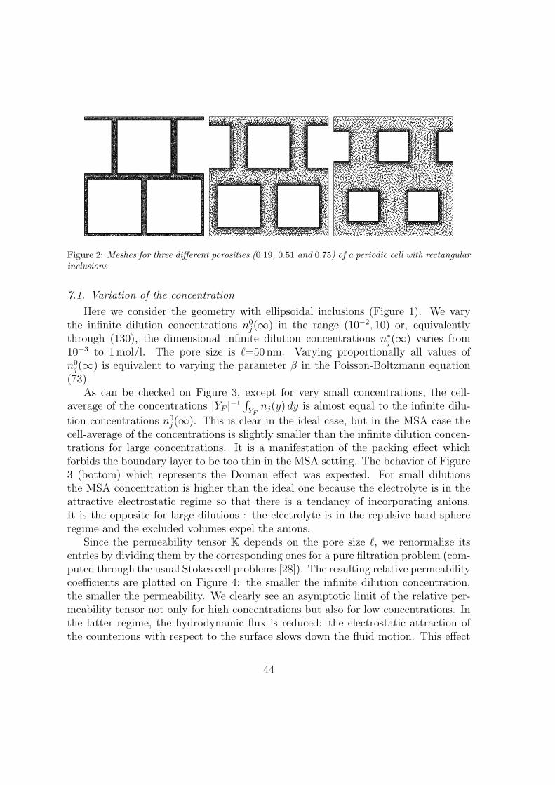
Figure 2: Meshes for three different porosities (0.19, 0.51 and 0.75) of a periodic cell with rectangularinclusions
7.1. Variation of the concentration
Here we consider the geometry with ellipsoidal inclusions (Figure 1). We varythe infinite dilution concentrations n0
j(∞) in the range (10−2, 10) or, equivalentlythrough (130), the dimensional infinite dilution concentrations n∗
j(∞) varies from10−3 to 1mol/l. The pore size is ℓ=50 nm. Varying proportionally all values ofn0j(∞) is equivalent to varying the parameter β in the Poisson-Boltzmann equation
(73).As can be checked on Figure 3, except for very small concentrations, the cell-
average of the concentrations |YF |−1∫YFnj(y) dy is almost equal to the infinite dilu-
tion concentrations n0j(∞). This is clear in the ideal case, but in the MSA case the
cell-average of the concentrations is slightly smaller than the infinite dilution concen-trations for large concentrations. It is a manifestation of the packing effect whichforbids the boundary layer to be too thin in the MSA setting. The behavior of Figure3 (bottom) which represents the Donnan effect was expected. For small dilutionsthe MSA concentration is higher than the ideal one because the electrolyte is in theattractive electrostatic regime so that there is a tendancy of incorporating anions.It is the opposite for large dilutions : the electrolyte is in the repulsive hard sphereregime and the excluded volumes expel the anions.
Since the permeability tensor K depends on the pore size ℓ, we renormalize itsentries by dividing them by the corresponding ones for a pure filtration problem (com-puted through the usual Stokes cell problems [28]). The resulting relative permeabilitycoefficients are plotted on Figure 4: the smaller the infinite dilution concentration,the smaller the permeability. We clearly see an asymptotic limit of the relative per-meability tensor not only for high concentrations but also for low concentrations. Inthe latter regime, the hydrodynamic flux is reduced: the electrostatic attraction ofthe counterions with respect to the surface slows down the fluid motion. This effect
44

is not negligible because the Debye layer is important. The MSA model differs fromthe ideal case. The curve is qualitatively the same but the electrostatic reductionof the Darcy flow is more important. Non ideality diminishes the mobility of thecounterions at the vicinity of the surface so that the electrostatic interactions in thedouble layers are more pronounced.
The entries of the electrodiffusion tensor D11 for the cation are plotted on Figure5. A similar behavior is obtained for the other tensor D22 for the anion. As expectedthe flux increases with the infinite dilution concentration n∗
j(∞). It is not a linear lawbecause even at low concentration there are still counterions ; they do not appear to bevery mobile, though. The cross-diffusion tensor D12 is displayed on Figure 6: for largeconcentrations it is of the same order of magnitude than the species diffusion tensorsD11 and D22, because of the strong electrostatic interactions between the ions. In allcases, the MSA model is close to the ideal one: it is only for large concentrations thatthe values of the electrodiffusion tensor are different, and smaller, for MSA comparedto ideal. There are probably compensating effects : same charge correlations increasediffusion but this effect is somewhat counterbalanced by opposite charge correlationsthat slow down the diffusion process. Non-ideal effects could be more important inthe case of further quantities such as the electric conductivity for which cross effectsare additive.
The log-log plot of Figure 7 (where the slope of the curve is approximately 2)shows that the electrodiffusion tensors Dji behaves quadratically as a function ofn∗j(∞) when n∗
j(∞) becomes large. This asymptotic analysis can be made rigorousin the ideal case. At low salt concentration, correlation effects (i.e. non-ideality)enhance slightly diffusion. In this regime, there are no counterions. So the relaxationeffect is purely repulsive and diffusion is enhanced [17]. At high concentration, theco-ion concentration is not negligible and there is a classical electrostatic relaxationfriction.
The coupling tensors L1 and L2 are plotted on Figure 8. The coupling is, ofcourse, maximal for large concentrations but the coupling tensor L1 for the cationdoes not vanish for very small infinite dilution concentrations since the cell-averageof the cation concentration has a non-zero limit (required to compensate the negativesurface charge) as can be checked on Figure 3. The differences between the ideal andMSA models are very limited in this logarithmic plot.
7.2. Variation of pore size
We keep the same geometry with ellipsoidal inclusions (Figure 1) but we now varythe pore size ℓ, which is equivalent to vary the parameter β, defined by (21), in thePoisson-Boltzmann equation (73). It thus changes the values of the concentrationsn0j(y) which play the role of coefficients in the cell problems (85)-(88) and (89)-(92).
45

This is the only modification which is brought into the cell problems. We emphasizethat varying the pore size does not change the geometry of the unit cell, but simplychanges the coefficients of the cell problems.
The dimensional infinite dilution concentration n∗1(∞) = n∗
2(∞) is 10−1 mol/lwhich yields a value 0.7678 for the infinite dilute activity coefficients γ10(∞) = γ20(∞).
On Figure 9 we plot the cell-average of the concentrations |YF |−1∫YFnj(y) dy as
functions of the pore size ℓ. Qualitatively, there is a close agreement between the idealand MSA cases, as can be checked on this logarithmic plot. Yet, the departure fromideality is not negligible. For small pore size the Donnan effect, which correspondsto the anion concentration, is typically 40 % higher than its value in the ideal case.When the pore size goes to infinity the averaged concentrations should converge tothe infinite dilution concentrations.
On Figure 10 we plot the relative permeability coefficients with respect to the onesof the Stokes problem. As was already observed in [6], the variation is not monotoneand there is a minimum for a pore size of roughly 20 nanometers. This effect is lesspronounced for the MSA model but the location of the ℓ value where the minimumis attained is not affected. This is the signature of a transition from a bulk diffusionregime for small pores to a surface diffusion regime (caused by large boundaries)at large pores. Globally, the counterions reduce the hydrodynamic flow because ofthe attraction with the surface, but this relaxation effect is less important at verylarge or very small pore size ℓ. More precisely, if the pore size becomes very large,the electrostatic screening is important, as already mentioned. Thus the domain ofattraction becomes very small and the lowering of the hydrodynamic flow is reduced:the permeability is increased. On the other hand, for very small pores, the counterionprofile becomes more and more uniform. Consequently, there is no screening, butthe hydrodynamic flow does not modify a lot the counterion distribution, since itis globally uniform and the resulting electrostatic slowdown becomes less important.The departures from ideality modelled by the MSA globally reduce the total variationof the permeability tensor because the mobility of the ions in the Debye layer is weakerand their dynamics influence less the Darcy flow.
7.3. Variation of the porosity
Eventually we investigate the influence of the porosity on the effective tensors.To this end we rely on the rectangular geometry where we vary the size of the in-clusions (see Figure 2). The infinite dilution concentration is fixed at n0
j(∞) = 1,or n∗
j(∞) = 0.1mol/l. The porosity is defined as |YF |/|Y | and takes the successivevalues of 0.19, 0.36, 0.51, 0.64, 0.75 in our computations. Note that the porosity isindependent of the pore size ℓ which is defined as the characteristic size of the entireperiodicity cell, i.e., the union of its fluid and solid parts. On Figure 11 we plot
46

the cell-average of the concentrations |YF |−1∫YFnj(y) dy as functions of the porosity.
They are almost identical between the ideal and MSA cases. When the porosity goesto 1, meaning that there are no more solid charged walls, the averaged concentrationsshould become equal, respecting the global electroneutrality. On Figure 12 we checkthat the permeability tensor is increasing with porosity, as expected. The same hap-pens for the electrodiffusion tensor D22 for the anion on Figure 14. More surprisingis the behavior of the electrodiffusion tensor D11 for the cation on Figure 13: againthere is a minimum value attained for a 0.35 value of the porosity. This may beexplained again by a transition from a bulk diffusion regime for large porosities to asurface diffusion regime (caused by the charged boundaries) for small porosities.
The departures from ideality are found to be very important. They multiply themagnitude of diffusion by a factor of two, especially at low porosities for which theamount of anions is low. It corresponds to the case for which the relaxation effect ispurely repulsive. A similar trend is obtained for the anion but the diffusion coefficientis much lower at low porosities: anions are expelled from the surface and they cannothave surface diffusion so that their transport properties are globally reduced.
8. Conclusion
We presented the homogenization (or upscaling) of the transport properties for aN -component electrolyte solution confined in a charged rigid porous medium. Con-trary to what is commonly supposed in this domain the departures from ideality areproperly taken into account thanks to a MSA-transport model, both for the equilib-rium properties (activity coefficients γj) and for the transport quantities (Onsagercoefficients Lij). These non ideal effects are expected to be significant in most ofthe applications for which the electrolyte concentrations are typically molar. In thecase of the equilibrium solution (in absence of external forces, apart from the surfacecharges on the solid wall), we prove the existence of (at least) one solution for smallsolute packing fractions (which corresponds to the validity of the MSA approach).
When a (small) external electric field is applied or when a (small) hydrodynamicor chemical potential gradient occurs, a rigorous homogenization procedure yields (atthe linear response regime) the homogenized macroscopic laws. The effective Onsagertensor takes into account the departure from ideality, but it is still symmetric andpositive definite. The significance of non-ideality has been studied by applying theresults to a model of porous media (typically geological clays) for simple dissociated1-1 electrolytes in water. It is shown that non-ideality only slightly modifies thequalitative aspects, but it can strongly modify the quantitative values, depending onthe homogenized quantities.
For the equilibrium properties, it enhances the ion concentrations at low external
47
concentration (because electrostatic attraction is predominant) and it reduces themat the opposite limit. The relative permeability tensor is increased but, in any case,it is close to the reference value calculated with a neutral solution. The differencesfor the coupled diffusions and ion electrodiffusions depend on the concentrations andon the species. Similarly to bulk diffusion, the non-ideality can have an impact ofthe order of 50 % for molar concentrations. Nevertheless, for some cases, there arecompensating effects. It should be noted that for the model we considered the charges(ions, solid phase) were relatively low so that the differences should be magnified forhighly charged media with higher valency electrolytes and higher concentrations. Inthat case, the result could be completely different because of the possibility of ionpairing that can change the sign of the ion charge. Nevertheless, the (relatively) simpleMSA-transport theory we presented is not valid anymore in that case so that a realisticquantitative description of such complex media would require further developments.
To conclude, we showed that non-ideality can actually be important for the de-scription of porous media. Since most of the existing effective theories for concen-trated systems are based on ideal models which neglect the departure from ideality,the parameters that can be measured thanks to these approaches may be wronglyestimated. In that case, they cannot be considered as robust structural quantities ofthe system: they are effective parameters that depend on the experimental conditions.
References
[1] P. M. Adler, V. Mityushev, Effective medium approximation and exact formulaefor electrokinetic phenomena in porous media, J. Phys. A: Math. Gen. 36 (2003),391-404.
[2] P. M. Adler, Macroscopic electroosmotic coupling coefficient in random porousmedia, Math. Geol. 33(1) (2001), 63-93.
[3] G. Allaire, Homogenization and two-scale convergence, SIAM J. Math. Anal., 23(1992), 1482-1518.
[4] G. Allaire, One-Phase Newtonian Flow, in Homogenization and Porous Media,ed. U.Hornung, Springer, New-York, (1997), 45-68.
[5] G. Allaire, A. Mikelic, A. Piatnitski, Homogenization of The Linearized IonicTransport Equations in Rigid Periodic Porous Media, Journal of MathematicalPhysics, 51, 123103 (2010). Erratum in the same journal, 52, 063701 (2011).
[6] G. Allaire, R. Brizzi, J.-F. Dufreche, A. Mikelic, A. Piatnitski, Ion transportin porous media: derivation of the macroscopic equations using upscaling andproperties of the effective coefficients, Comp. Geosci., 17, Issue 3, 479-495 (2013).
48

[7] G. Allaire, J.-F. Dufreche, A. Mikelic, A. Piatnitski, Asymptotic analysis of thePoisson-Boltzmann equation describing electrokinetics in porous media, Nonlin-earity, 26 (2013) 881-910.
[8] J. L. Auriault, T. Strzelecki, On the electro-osmotic flow in a saturated porousmedium, Int. J. Engng Sci. 19 (1981), 915-928.
[9] J. M. G. Barthel, H. Krienke, W. Kunz, Physical Chemistry of Electrolyte Solu-tions, Springer, (1998).
[10] A. Bensoussan, J. L. Lions, G. Papanicolaou, Asymptotic analysis for periodicstructures, volume 5 of Studies in Mathematics and its Applications. North-Holland Publishing Co., Amsterdam (1978).
[11] O. Bernard, W. Kunz, P. Turq, L. Blum, Conductance in Electrolyte SolutionsUsing the Mean Spherical Approximation, J. Phys. Chem. 96 (1992), 3833.
[12] L. Blum J.S. Hoye: Mean Spherical Model for Asymmetric Electrolytes. 2. Ther-modynamic Properties and the Pair Correlation, J. Phys. Chem. 81 (1977), 1311.
[13] D.Y. Chan, R.G. Horn, The drainage of thin liquid films between solid surfaces,J. Chem. Phys. 83 (1985), 5311-5325.
[14] D. Coelho, M. Shapiro, J.-F. Thovert, P. M. Adler, Electro-osmotic phenomenain porous media, J. Colloid Interface Sci. 181 (1996), 169-90.
[15] S. Van Damme, J. Deconinck, Relaxation Effect on the Onsager Coefficients ofMixed Strong Electrolytes in the Mean Spherical Approximation, J. Phys. Chem.111 (2007), 5308.
[16] J.-F. Dufreche, V. Marry, N. Malikova, P. Turq, Molecular hydrodynamics forelectro-osmosis in clays: from Kubo to Smoluchowski, J. Mol. Liq. 118 (2005),145.
[17] J.-F. Dufreche, O. Bernard, P. Turq, A. Mukherjee, B. Bagchi, Ionic self-diffusionin concentrated aqueous electrolyte solutions, Phys. Rev. Lett. 88 (2002), 095902.
[18] J.-F. Dufreche, M. Jardat, T. Olynyk, O. Bernard, P. Turq, Mutual diffusion co-efficient of charged particles in the solvent-fixed frame of reference from Browniandynamics simulation, J. Chem. Phys. 117 (2002), 3804.
[19] J.-F. Dufreche, O. Bernard, S. Durand-Vidal, P. Turq, Analytical Theories ofTransport in Concentrated Electrolyte Solutions from the MSA, J. Phys. Chem.B 109 (2005), 9873.
49

[20] J.-F. Dufreche, O. Bernard, P. Turq, Transport equations for concentrated elec-trolyte solutions: reference frame, mutual diffusion, J. Chem. Phys. 116 (2002),2085.
[21] W. Ebeling, J.Rose, Conductance Theory of Concentrated Electrolytes in anMSA-Type Approximation, J. Sol. Chem. 10 (1981), 599.
[22] D. A. Edwards, Charge transport through a spatially periodic porous medium:electrokinetic and convective dispersion phenomena, Philos. Trans. R. Soc. Lond.A 353 (1995), 205-242.
[23] I. Ekeland, R. Temam, Analyse convexe et problemes variationnels, Dunod,Gautier-Villars, Paris (1979).
[24] A. Ern, R. Joubaud, T. Lelievre, Mathematical study of non-ideal electrostaticcorrelations in equilibrium electrolytes, Nonlinearity 25 (2012), 1635-1652.
[25] S. R. de Groot, P. Mazur, Non-Equilibrium Thermodynamics, North-Holland,Amsterdam (1969).
[26] A.K. Gupta, D. Coelho, P.M. Adler, Electroosmosis in porous solids for high zetapotentials, Journal of Colloid and Interface Science 303 (2006), 593-603.
[27] J.-P. Hansen, I. R. McDonald, Theory of Simple Liquids, Academic Press, (1986).
[28] U. Hornung, editor. Homogenization and porous media, volume 6 of Interdisci-plinary Applied Mathematics, Springer-Verlag, New York (1997).
[29] M. Jardat, J.-F. Dufreche, V. Marry, B. Rotenberg, P. Turq, Salt exclusion incharged porous media: a coarse-graining strategy in the case of montmorilloniteclays, Phys. Chem. Chem. Phys. 11 (2009), 2023.
[30] R. Joubaud, Modelisation mathematique et numerique des fluides a lechellenanometrique, PhD thesis, Universite Paris Est (2012).
[31] G. Karniadakis, A. Beskok, N. Aluru, Microflows and Nanoflows. Fundamentalsand Simulation, Interdisciplinary Applied Mathematics, Vol. 29, Springer, NewYork (2005).
[32] J.-L. Lions, Some methods in the mathematical analysis of systems and theircontrols, Science Press, Beijing, Gordon and Breach, New York (1981).
[33] R. Lipton, M. Avellaneda, A Darcy Law for Slow Viscous Flow Past a StationaryArray of Bubbles, Proc. Royal Soc. Edinburgh 114A, (1990), 71-79.
50

[34] J.R. Looker, Semilinear elliptic Neumann problems and rapid growth in the non-linearity, Bull. Austral. Math. Soc., Vol. 74, no.2, (2006), 161-175.
[35] J.R. Looker, S.L. Carnie, Homogenization of the ionic transport equations inperiodic porous media, Transp. Porous Media 65 (2006), 107-131.
[36] J. Lyklema, Fundamentals of Interface ans Colloid Science, Academic Press,(1995).
[37] S. Marino, M. Shapiro, P.M. Adler, Coupled transports in heterogeneous media,J. Colloid Interface Sci. 243 (2001), 391-419.
[38] V. Marry, J.-F. Dufreche, M. Jardat P. Turq, Equilibrium and electrokineticphenomena in charged porous media from microscopic and mesoscopic models:electro-osmosis in montmorillonite, Mol. Phys. 101 (2005), 3111.
[39] C. Moyne, M. Murad, Electro-chemo-mechanical couplings in swelling clays de-rived from a micro/macro-homogenization procedure, Int. J. Solids Structures 39(2002), 6159-6190.
[40] C. Moyne, M. Murad, Macroscopic behavior of swelling porous media derivedfrom micromechanical analysis, Transport Porous Media 50 (2003), 127-151.
[41] C. Moyne, M. Murad, A Two-scale model for coupled electro-chemomechanicalphenomena and Onsager’s reciprocity relations in expansive clays: I Homoge-nization analysis, Transport Porous Media 62 (2006), 333-380.
[42] C. Moyne, M. Murad, A two-scale model for coupled electro-chemo-mechanicalphenomena and Onsager’s reciprocity relations in expansive clays: II. Computa-tional validation, Transp. Porous Media 63(1) (2006), 13-56.
[43] C. Moyne, M. Murad, A dual-porosity model for ionic solute transport in expan-sive clays, Comput Geosci 12 (2008), 47-82.
[44] G. Nguetseng, A general convergence result for a functional related to the theoryof homogenization, SIAM J. Math. Anal. 20(3), 608-623 (1989).
[45] R. W. O’Brien, L. R. White, Electrophoretic mobility of a spherical colloidalparticle, J. Chem. Soc., Faraday Trans. 2 74(2) (1978), 1607-1626.
[46] O. Pironneau, F. Hecht, A. Le Hyaric, FreeFem++ version 3.8,http://www.freefem.org/ff++/.
51

[47] N. Ray, Ch. Eck, A. Muntean, P. Knabner, Variable Choices of Scaling in theHomogenization of a Nernst-Planck-Poisson Problem, preprint no. 344, Institutfur Angewandte Mathematik, Universitaet Erlangen-Nurnberg (2011).
[48] N. Ray, A. Muntean, P. Knabner, Rigorous homogenization of a Stokes-Nernst-Planck-Poisson system, J. Math. Anal. Appl. 390(1) (2012), 374-393.
[49] R. A. Robinson, R. H. Stokes, Electrolyte Solutions, Butterworths, London(1970).
[50] M. Rosanne, M. Paszkuta, P.M. Adler, Electrokinetic phenomena in saturatedcompact clays, Journal of Colloid and Interface Science, 297 (2006), 353-364.
[51] B. Rotenberg, I. Pagonabarraga, Electrokinetics: insights from simulation on themicroscopic scale, Mol. Phys. 111 (2013), 827.
[52] E. Sanchez-Palencia, Non-Homogeneous Media and Vibration Theory, LectureNotes in Physics 127, Springer Verlag, (1980).
[53] M. Schmuck, Modeling And Deriving Porous Media Stokes-Poisson-Nernst-Planck Equations By A Multiple-Scale Approach, Commun. Math. Sci. 9 (2011),no. 3, 685-710.
52

Figure 3: Averaged cell concentrations Nj mean = |YF |−1∫YF
nj(y) dy (top) and rescaled averaged
cell anion concentration N2 mean/n02(∞) (bottom) as a function of the dimensional (mol/l) infinite
dilution concentrations n∗j (∞)
53

Figure 4: Diagonal entries of the relative permeability tensor, K11 and K22, as functions of thedimensional (mol/l) infinite dilution concentrations n∗
j (∞)
Figure 5: Entries of the electrodiffusion tensor D11 for the cation, as functions of the dimensional(mol/l) infinite dilution concentrations n∗
j (∞)
54
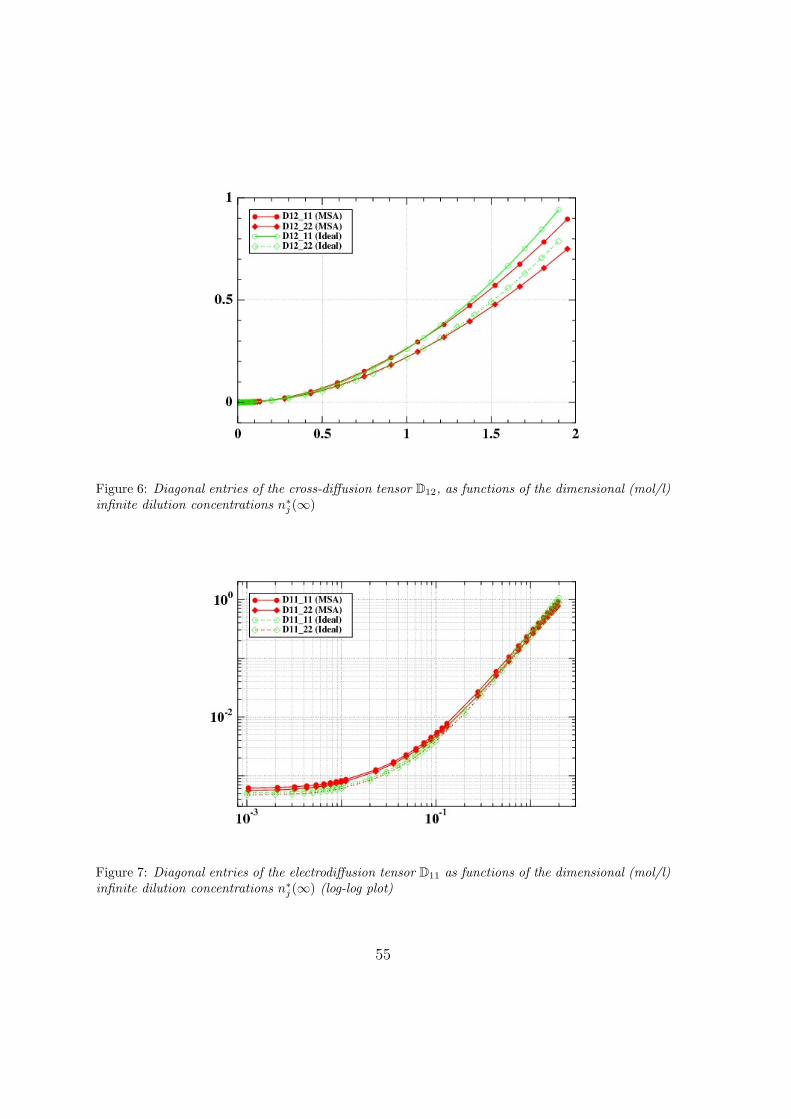
Figure 6: Diagonal entries of the cross-diffusion tensor D12, as functions of the dimensional (mol/l)infinite dilution concentrations n∗
j (∞)
Figure 7: Diagonal entries of the electrodiffusion tensor D11 as functions of the dimensional (mol/l)infinite dilution concentrations n∗
j (∞) (log-log plot)
55

Figure 8: Diagonal entries of the coupling tensors L1 and L2, as functions of the dimensional (mol/l)infinite dilution concentrations n∗
j (∞) (log-log plot)
56

Figure 9: Averaged cell concentration Nj mean = |YF |−1∫YF
nj(y) dy versus pore size ℓ (nm)
Figure 10: Relative permeability coefficients K11 and K22 versus pore size ℓ (nm)
57

Figure 11: Averaged cell concentration Nj mean = |YF |−1∫YF
nj(y) dy versus porosity (n∗j (∞) =
0.1mole/l)
Figure 12: Permeability tensor K versus porosity (n∗j (∞) = 0.1mole/l)
58
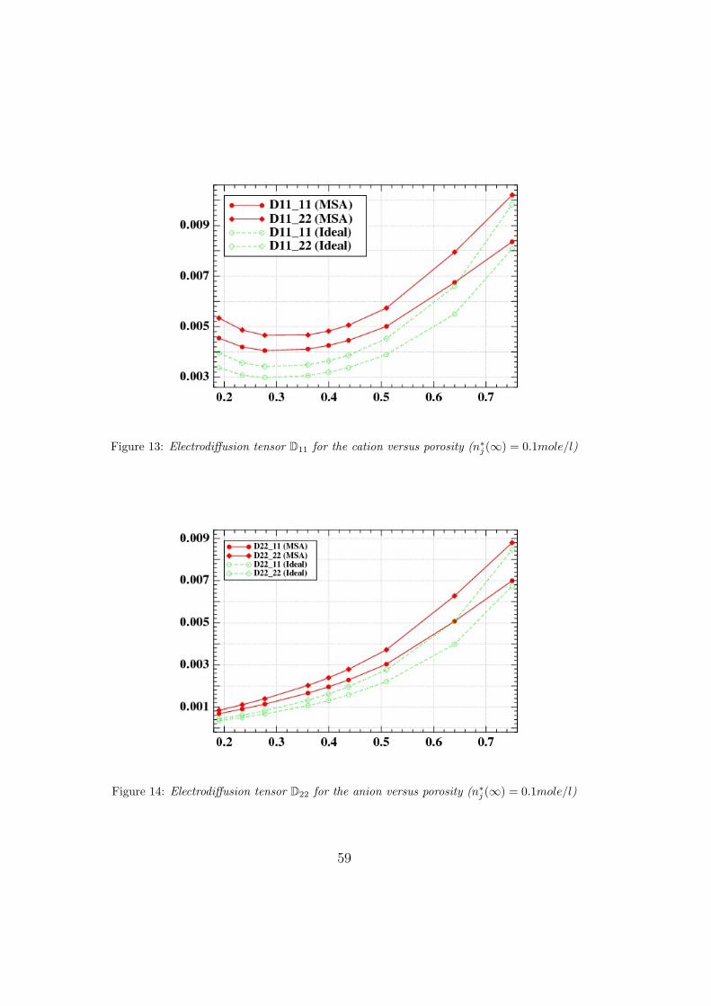
Figure 13: Electrodiffusion tensor D11 for the cation versus porosity (n∗j (∞) = 0.1mole/l)
Figure 14: Electrodiffusion tensor D22 for the anion versus porosity (n∗j (∞) = 0.1mole/l)
59