rock breaks scissors - reference guide

The Zenith Broadcast

29

success in demonstrating telepathy, clairvoyance, and telekine-sis. With piercing eyes and a dramatic sweep of steely hair, Rhine — a botanist by training — was a compelling advocate. He received mostly favorable attention in publications ranging from the New Yorker to Scientific American. As one journalist condescended, Rhine made ESP “the brief rage of women’s clubs all over the U.S.”

On a balmy June night, Rhine and his wife had dinner aboard McDonald’s yacht. McDonald sketched his idea for a nationwide test of ESP by radio. Listeners could test their own psychic powers. It would be the biggest experiment ever, pro-viding the best possible proof that telepathy was real.

Rhine was not sure that his newborn science was ready for prime time. Skeptics suspected that Rhine was reporting suc-cesses and ignoring failures — that some of his telepaths were cheating.

The skeptics didn’t worry McDonald. As one of his associ-ates put it, “nothing stops a crowd on a street like a fight.” McDonald played Mephistopheles, tempting Rhine with plans to monetize telepathy. He said he’d have his attorneys look into copyright and trademark protection for the cards that Rhine used to test ESP. This was the so-called Zener deck, named for a colleague, marked with five symbols (circle, cross, wavy lines, square, and star). Rhine would get a royalty on every pack sold,

RockBreaksScis_HCtext3P.indd 29 12/21/13 3:17:20 AM

Rock Breaks Scissors

46

think. Mentalists play the odds and usually have ways of sneak-ing in a few more guesses, should the first one not hit. They accept a chance of failure. J. B. Rhine unwittingly helped out there by promoting the credo that telepathy is never 100 per-cent. Audiences, who are often uncertain whether a mentalist’s powers are “real,” take the occasional miss as a badge of authenticity.

I’ll describe a mentalism effect I witnessed that illustrates some of the tactics that we’ll be using throughout this book. It goes by the name of Terasabos. The performer calls an audi-ence volunteer onstage and positions him at one end of a table with five upside- down teacups in a neat row. He asks for a per-sonal object, like a watch, and the volunteer supplies one. The mentalist says he is going to turn his back and let the volunteer hide the watch under any one of the cups, ranging from one to five. He demonstrates the action — lift up a cup, put the object under it, and replace the cup.

Then he turns his back. There doesn’t appear to be any possibility of his peeking, not with everyone in the audience watching him. The volunteer chooses a cup (say, #4) and hides the watch under it.

The performer turns around and instructs the volunteer to concentrate on the location of the watch. He says he has to elim-inate the four cups where the watch isn’t, and to zero in on the one where it is. For a few moments he stares intently at the cups.

Then ultimately the performer lifts cup #4, revealing the hidden watch.



52

$17.8 million, earning the auction house a $1.9 million commission.

In college I knew a guy who had made a study of rock, paper, scissors. He assured me that the game was not as trivial as it seemed, and as proof he taught me a rather diabolical trick for winning bar tab bets with it. Good RPS players do what the outguessing machine did. They attempt to recognize and exploit unconscious patterns in their opponents’ play. That is anything but trivial. A World Rock Paper Scissors Society holds tournaments in Toronto. Though the media inevitably slots it under “news of the weird,” the coverage is usually deep enough to acknowledge the psychological elements.

The strategy for playing RPS depends on how skilled your opponent is. Let me start by giving a basic strategy for playing against a novice player (which is to say, 99 percent of the public).

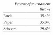
First of all, the throws are not equally common. The World RPS Society reports these proportions (for tournament play, with mostly expert players).

Percent of tournament throws

Rock 35.4%

Paper 35.0%

Scissors 29.6%

Though the names of the throws are arbitrary, they inherit cultural stereotypes. Rock is the testosterone choice, the most aggressive and the one favored by angry players. The majority of participants in RPS tournaments are male (is this a surprise


How to Outguess Multiple- Choice Tests

59

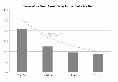
The other finding is that, as expected, there is more true- false- true- false alternation than in a properly random sequence. For example, here’s the answer key to a twenty- item test from a college textbook (Plummer, McGeary, Carlson’s Physical Geology, ninth edition): FTTFTFFTTFTTFTTTFTTF. I’ll display it as a series of black and white squares, with white representing true items.

This is not as random as it looks. One way to judge ran-domness is to count how many times a correct answer (true or false) is followed by the same correct answer. This occurs just seven times out of nineteen (the twentieth answer has no suc-cessor). To put it another way, the chance that the next answer will be different from the present one is 63 percent. That’s more than the expected 50 percent for a random sequence.

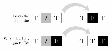
You won’t be guessing on every item, let’s hope. For the most part you will know the correct answers to the questions before and after the difficult ones. That permits this true- false test strategy:

Go through the entire test, marking the answers you know, before attempting to make any guesses.

Look at the known correct answers of the items before and after the one(s) that’s left you stumped. When both neigh-boring answers are the same (both false, let’s say), guess the opposite (true).

Should the before and after answers be different, guess true (because true answers are more likely overall).

Example. You have to guess on an item that is surrounded by items you’re sure are true. You’re better off guessing false.

When one neighboring answer is true and the other is



60

false, the alternation rule gives conflicting signals. You should default to the more common answer, true.

There is a rich folklore on multiple- choice test guessing. I remember being advised to pick the center choice. Based on my data, that tactic wouldn’t do much good. On tests with three choices (call them A, B, and C), the options were about equally likely to be correct. With four options, the second answer (B) was favored, being correct about 28 percent of the time. That’s compared to the expected 25 percent for four answers.

With five options, the last answer (E) was the most com-monly correct one (23 percent). The middle choice (C) was the least favored (17 percent).

It appears that test makers intuitively get the proportions right for three choices but have trouble doing so when there are more than three. This is in line with experimental findings that the quality of randomizing decreases as the number of options increases.

A better guessing policy would be to pick the second answer (B) on four- choice tests and the fifth answer (E) on five- choice tests.


How to Outguess Multiple- Choice Tests

63

gain an easy advantage when guessing just by avoiding the pre-vious question’s answer.

I rated that and other multiple- choice strategies by calcu-lating how much they improved on random guessing.

StrategyImprovement on Random Guessing

Pick the “none of the above” or “all of the above” answer 90%

Pick B on a four- choice test, E on a five- choice test 11%

Avoid the previous choice 8%

Hands down, the best strategy was picking “none of the above” or “all of the above.” These choices were almost twice as likely to be true as other choices, offering a 90 percent



64

improvement on random guessing. (A few questions offer both “none” and “all” answers. Unless you’re totally at sea, you should be able to rule one out.)

Guessing the most common positional choice and avoid-ing the previous correct choice were also successful. They were about equally effective, particularly when you figure that you can boost the “avoid the previous choice” success rate a bit by also avoiding the following question’s correct answer.

Whenever you have to guess on a multiple- choice ques-tion, you should first eliminate any options you can. Knowl-edge trumps outguessing! If there’s a “none”/“all” choice that you can’t rule out, pick it. Otherwise, use the two other rules.

Example. You don’t know the answer to question #2, though you’re sure the third one (C) is wrong. That leaves three open possibilities. There is no “all of the above” or “none of the above” answer.

The second choice is most often correct for a four- choice question, so that’s one vote for B. Make an imaginary check-mark next to it.

You know that the correct answers to the neighboring questions, #1 and #3, are C and D. That’s reason to favor a dif-ferent choice here — A or B. Place checkmarks next to them.

This gives us one vote for A, two for B, none for D — and C is ruled out on factual grounds. B is the best guess.

When “voting” leads to a tie, pick any of the tied options.


How to Outguess the Lottery

75

For the Mega Millions and Powerball, use all the numbers in the chart, and draw five. Then replace the drawn numbers in the deck for the second- barrel pick. For Powerball, you’ll be using only the first five numbers in the chart. For Mega Mil-lions, ten is probably the best choice for the gold Mega Ball.

2. Now you’ve got six legal picks of relatively unplayed numbers. Make sure they don’t happen to make a geometric pattern on the physical or virtual play slip. Indecisive bettors often default to picking numbers that form a line or other pat-tern on the play slip. Diagonals are especially popular because they seem more random. Vertical lines are also used, and occa-sionally people pick a cross of five numbers (which could be horizontal- vertical or diagonal).

In the unlikely event that your picks form a pattern, you should either start over or swap one of your picks with another unpopular number, to eliminate the pattern.

3. Should it come to your attention that a popular TV show or movie or book or video game has mentioned a set of pick-six numbers, avoid them. Avoid numbers that are in the news.



82

mental pie slices probably capture your intuition as well as guesstimated numbers could. They also save time. You don’t have to invent a percentage number and then convert that to a percentage of a clock dial. You just go with what looks right.

Recap: How to Outguess Tennis Serves

Expect the direction of serve to alternate, especially with novice players.

When playing a good opponent, use a watch or heart- rate monitor to randomize your own serves.



94

It’s not hard to read pupils, but you have to be looking directly at the person’s eyes when the change occurs. The change is fast enough to see, and you are looking for that change rather than the pupils’ absolute size (which varies with room lighting and drug use). A typical positive reaction is a 10 percent increase in the diameter of both pupils (a 20 percent increase in area). A bad turn of luck may cause the pupils to shrink. It looks like this, roughly actual size:

The change takes place in the half second or so after the player sees a fateful card. Not surprisingly, some serious players wear dark glasses as a countermeasure.

Recap: How to Outguess Card Games

When card players make strategic random decisions, they avoid streaks of the same choice. A player who bluffs this time is less likely to bluff on the next weak hand.

You might want to use a watch to randomize your bluffing, but be sure to glance at the watch with every hand.

A good pupil reader can tell whether you drew the card you needed — if he can see your eyes.


How to Outguess Passwords

105

Here are Berry’s twenty most common PINs:

1234 99991111 33330000 55551212 66667777 11221004 13132000 88884444 43212222 20016969 1010

All the four- identical- digit choices appear. This isn’t a ran-domness experiment, it’s an I’m-afraid-I’ll- forget- this- number- and- better- pick- something- really- easy experiment.

Berry found these less obvious patterns:

Years. All recent years and a few from history (1492, 1776) are high up on the list.Couplets. Many pick a two- digit number and clone it to get the needed four (1212, 8787, etc.) Digits in couplets most often differ by 1.2580. Some figure they’ll generate a random code by playing tic- tac- toe on the keypad. The only way to get the required four digits is to go straight down the mid-dle: 2580. It’s the twenty- second- most- popular choice in Berry’s list. (For that you can thank the designer of the keypad, Alphonse Chapanis.)1004. In Korean the numbers sound like the word for angel. This inspired a pop tune, “Be My 1004.” There


How to Outguess Fake Numbers

113

the digit 1. In contrast, only about 5 percent of the numbers started with 9. This left the back part of the book relatively pristine.

Benford mentioned this fact to GE chemist Irving Lang-muir (later a Nobel laureate). Langmuir encouraged him to publish a paper on it. Methodical if nothing else, Benford pur-sued this obscure finding over the next decade. It was not, he found, unique to scientific numbers. He tried tallying the first digits of baseball statistics and found the same distribution. He recorded every number mentioned in an issue of Reader’s Digest. Ditto. Tennis scores, stock quotes, lengths of rivers, atomic weights, electric bills in the Solomon Islands, and numbers mentioned on the front page of the New York Times produced the same pattern. It was like a conspiracy theory. Everything was connected.

Benford finally published his results in a 1938 issue of the Proceedings of the American Philosophical Society. There he derived a precise formula for the proportion of numbers begin-ning with each digit. The proportions are:

First digit Proportion

1 30.1%

2 17.6%

3 12.5%

4 9.7%

5 7.9%

6 6.7%

7 5.8%

8 5.1%

9 4.6%



117

Varian had not followed up his idea, nor had anyone else. This stoked Nigrini’s enthusiasm, though not that of his advi-sor. “They prefer you to be the eightieth person to write about a topic,” Nigrini explained. He went ahead with his dissertation anyway. Not until he had written two- thirds of the research was he able to get it approved. He finished it four months later.

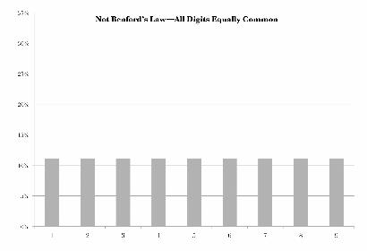
The idea that struck Varian and Nigrini lends itself to a picture. When you have a lot of numbers, you can make a bar chart (histogram) showing how many times each digit occurs as the first digit. Just count how many of the numbers start with the digit 1, how many start with 2, 3, and so on. For honest data that follows Benford’s law, the chart will look like this:

This smooth curve is Benford’s law in visual form.Varian and Nigrini’s brainstorm was that people who

make up numbers won’t know about Benford’s law. An embez-zler or tax cheat will have no reason to think that any digit should be more common than any other. Therefore, a set of



118

made-up numbers might be expected to show an even distribu-tion of leading digits, without the curve.

That was the back-of- the- envelope concept, anyway. Ran-domness experiments (which were not widely known) had already shown that fabricated numbers almost never use all digits equally. Alphonse Chapanis made bar charts of his results, and they didn’t look anything like a flat distribution.

Another issue is that honest financial data often fits the Benford curve to a T — and then sometimes it doesn’t. It can be tough to tell beforehand which case you’re dealing with. One example would be sales data from the 99 cents store. The amounts would include a lot of 9s. As Nigrini points out, this tells you that prices are made-up numbers, invented by humans as part of a mar-keting strategy. But if you’re managing a 99 cents store, that’s your reality, and it doesn’t indicate fraud. There are many other situa-tions where the nature of a business might produce an un- Benford- like distribution of first digits, for perfectly innocent reasons.



119

Nigrini’s basic idea was right, though: Invented num-bers are different from honest ones. He began to haunt the Cin-cinnati courthouse, looking for criminal cases involving numbers.

One of the early fraud cases he studied was from Arizona. Wayne James Nelson, a forty- three- year- old manager in the office of the Arizona state treasurer, launched a short embez-zling career with a check for $1,927.48 from the State of Arizona to a fictitious vendor. Over the next few days he made twenty- two more fake checks, for a total of almost $1.9 million.

When caught, Nelson claimed that he had written the checks in a noble effort to demonstrate vulnerabilities in Ari-zona’s accounts payable system. He had “neglected” to enlighten anyone in the treasurer’s office about these vulnerabilities, and the funds had been directed to Nelson’s own accounts.

At a glance, you can see some patterns in Nelson’s check amounts.

$1,927.48 $96,879.27$27,902.31 $91,806.47

$86,241.90 $84,991.67

$72,117.46 $90,831.83

$81,321.75 $93,766.67

$97,473.96 $88,338.72

$93,249.11 $94,639.49

$89,658.17 $83,709.28

$87,776.89 $96,412.21

$92,105.83 $88,432.86

$79,949.16 $71,552.16

$87,602.93



120

Nelson “was the anti- Benford,” said Nigrini. All but the first two check amounts start with high digits 7, 8, and 9. Nel-son kept the amounts under $100,000, probably because six- figure sums would have attracted unwelcome attention.

Here’s a histogram of the leading digits of Nelson’s check amounts.

Dodgy numbers are usually mixed in with legitimate ones. An auditor would not just be looking at the fake check amounts (how would he know which were fake?). He would look at all of Nelson’s check amounts, or all of his department’s amounts. Even so, Nelson’s lopsided preference for 8s and 9s in the fake amounts would augment the 8s and 9s in the aggregate amounts. This might be detectable.

Nigrini found that Nelson’s check amounts showed other idiosyncrasies typical of invented numbers. Suppose we tally the very last (rightmost) digits of the check amounts. These



121

represent pennies, and surely Nelson had no financial interest in that. There is a pattern nonetheless. Nelson favored amounts ending in 6 and 7. He didn’t use 4 at all.

This looks much like the charts that Chapanis made. Just like Chapanis’s volunteers, Nelson unconsciously repeated him-self. In twenty- three check amounts, he managed to repeat 87, 88, 93, and 96 as the first two digits. He likewise repeated the cents figures 16, 67, and 83.

The IRS sells tax form data, with identifying information stripped out, to researchers. Nigrini bought a package of 100,000 returns for tax years 1985 and 1988 and began analyz-ing them on the university’s VAX minicomputer. He wanted to see whether he could tell which entries had the most cheating.

Many entries on a tax form are calculated totals, differ-ences, or products of other entries. It would make no sense to



127

sales or ten years of weekly figures. Even with 500 numbers, the chart is noisy, with a great deal of variation. In this case, there’s a pair (68) that doesn’t occur at all in the data, and three pairs (10, 53, 74) that occur twice as much as the expected 1 per-cent. This is the normal variation you should expect for ran-dom data.

Now let’s look at fabricated data.The chart on the next page shows the last two digits of 500

human- invented numbers. Even at a glance you can see there’s a lot more variation. Two pairs (93 and 94) occur more than 4 percent of the time, something very unlikely with honest num-bers. Twelve pairs don’t occur at all, and that’s also highly improbable.

Ask the following three questions. A “yes” answer to any of the three should raise the suspicion level.



128

(a) Is there a pair (or pairs) that is unaccountably more common than the others?

(b) Are doubled digits (especially 00 and 55) consistently less common than average?

(c) Are descending pairs (10, 21, 32, 43, 54, 65, 76, 87, 98) consistently more common?

In the example here, the answer to (a) is a resounding yes. The data also avoids doubled digits (b). You would expect that 10 percent of all numbers would end in a pair of doubled digits. Here are 20 occurrences out of 500, only 4 percent. The pairs 00, 55, and 77 do not occur at all.

There are 44 descending pairs out of 500. That’s almost exactly the expected 9 percent (as there are nine descending pairs out of 100 possibilities). By criterion (c) the data is unsuspicious.



132

the first time you see something like this. An employee who knows that the company will reimburse meals up to $50 may try to run tabs of $49 and change. She’s not doing the company any favors, but she’s playing by the rules that the company set up.

On the other hand, an employee who overreports meal expenses — or makes them up — has reason to lurk under the threshold, too. With a result like this, you might want to check on whether the employee submitted receipts for the just- below- threshold amounts, whether they match, and whether there is any sign of tampering.

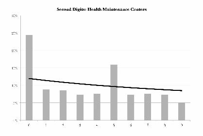
Occasionally thresholds end in 5, such as $25. In that case manipulation will produce an excess of 3s and 4s as second digits.

Kevin L. Lawrence came to investors with a can’t-lose business plan. His company, Health Maintenance Centers (HMC), was developing electronics and software to allow health clubs to monitor their members’ performance on exercise equipment. It



134

menu of round amounts. When we make up dollar amounts, and aren’t trying to deceive anyone by making them look ran-dom, we almost always pick round numbers.

The only thing wrong with round numbers is that, in some contexts, they aren’t businesslike. Companies have a responsibility to negotiate the best deals and to buy no more than is needed. Even when a price happens to be a round num-ber, a Brownian motion of discounts, allowances, transporta-tion charges, and taxes tends to move the net amount away from the round number. The discipline of running an honest business exerts a gravitational pull, bringing the associated dollar values into line with Benford’s law. When the money handling is more lax or evasive, the dollar values diverge.

HMC’s principals had been using its funds like a personal checking account. Or an ATM machine, literally. A total of 111 of HMC’s payments turned out to be for $301.50. Employees had been given ATM cards to draw on HMC’s accounts. The


How to Outguess Manipulated Numbers

135

maximum withdrawal permitted was $300, and the bank tacked on a $1.50 fee.

An excess of $10, $15, $20, and $25 charges was due to bank fees for cashier’s checks and wire transfers. These services are intended for individuals. Companies have cheaper ways to move funds. At the very least, this shows that HMC’s employees weren’t interested in saving the investors’ money. It also raises the question, why weren’t HMC’s own checks good enough?

The answer was also to be found in the numbers. Another bump came from a fee for bounced checks.

The investigation concluded that HMC was using checks and transfers to shift large round- number amounts from one dubious entity to another, most of it eventually landing in the pockets of HMC’s principals. The financial shell game was probably intended to make it hard to follow what was going on.

In the five years leading up to its collapse, Enron, the notoriously fraudulent energy company, reported these revenue figures:

1996 $13.289 billion

1997 $20.273 billion

1998 $31.260 billion

1999 $40.112 billion

2000 $100.789 billion

In hindsight, we know that these numbers were a fiction woven by chief financial officer Andrew Fastow. Enron’s manag-ers had become mesmerized by the Pavlovian connection between revenue and stock price. The stock price was posted in the com-pany’s elevator. Fastow found ways to report the revenues to jus-tify the stock prices that everyone at the company desired.



136

Enron president Jeffrey Skilling spent much of his work-day rebutting doubting Thomases. In a now- famous conference call, Highfields Capital analyst Richard Grubman remarked that Enron was the only company he knew that did not pro-duce a balance sheet or cash flow statement with its earnings. “Well, thank you very much,” Skilling replied. “We appreciate it . . . asshole!”

The few figures that Enron did release were suspicious enough. When a company is on track to sell a million widgets, 998,300 will be a disappointment. Three of the five revenue figures just top a psy-chologically potent round number — of $20, $40, and $100 billion.

Each of Enron’s threshold- beating numbers has a second digit of 0. Benford’s law predicts that the chance of a number’s second digit being 0 is 11.97 percent. When you get several nar-rowly threshold- beating numbers in proximity, the odds grow longer. The chance of three out of five numbers having a second digit of 0 is about 1 in 75.

Revenue is a headline number, one likely to be featured in the financial media. There aren’t many headline numbers, but they’re the ones that drive stock prices. Another widely reported number is earnings per share. Here are Enron’s:

1996 $1.08

1997 $0.16

1998 $1.01

1999 $1.10

2000 $1.12

Earnings were a lot less impressive than revenue. Enron was straining to make a dollar a share, and there’s scant indica-tion of growth over five years. The outlier year was 1997. “Oper-



152

able to collect it. That averages out to a 10.6 percent annual return.

More eyebrow- raising was how steady the claimed returns were. The chart shows the value of a dollar invested in Fairfield Sentry against a dollar invested in the S&P 500 index. Fairfield Sentry was not only steadier than a stock index but steadier than US Treasury bonds.

Madoff knew all about volatility. But when he came to invent fake numbers, he fell back on the not-so-rational instincts we all share. He apparently felt a need to keep monthly returns close to the average he was pitching. Only once (Janu-ary and February 2003) did he deliver two negative returns in a row.

You might look at the chart and say that returns can’t be that consistent. Then you wouldn’t have put your money with Madoff, and that would have been the right call. Fairfield Sen-



154

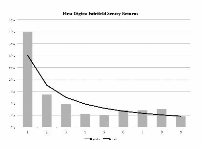
Forty percent of the returns start with 1. That’s well beyond the 30 percent predicted by Benford’s law. The digits 2 through 5 are underrepresented, and there’s an excess of 7s and 8s. These differences are statistically meaningful.

Madoff was claiming returns of about 11 percent a year. That means the monthly returns would tend to be close to 1 percent. These returns were rock steady, never straying too far from the mean. Take all that at face value, and you’d expect a disproportionate number of months with returns in the range of 0.70 to 1.99 percent. That would create an excess of first dig-its of 7, 8, 9, and 1, and a deficit of the other digits.

That’s what we do see, with one exception. The first digit 9 occurs in just about the Benford proportion. This contrasts with the greater- than- Benford occurrence of the digits around it.

A likely explanation is manipulation. Like everybody else, Madoff knew that a return of 1.00+ percent feels a lot bigger


How to Outguess Ponzi Schemes

155

than one of, say, 0.99 percent. So he avoided 9s. Monthly returns that otherwise might have started with 9 were bumped up to 1.00+ percent. It’s difficult to think of an alternative explana-tion even if you buy Madoff ’s claim of fantastically low volatility. Why else would steady returns skip over values starting with 9?

Now let’s look at the last two digits of the monthly returns. The chart of last two digits, from 00 to 99, shows a ragged picket fence with some slats missing. Several digit pairs are far more common than the others. The chart’s most remarkable feature is the spike for 86. Those are the last two digits for eight of Fair-field Sentry’s monthly returns. There are also three pairs that occur 6 times: 14, 26, and 36.

This is consistent with the unconscious repetition of invented numbers. This idea becomes more compelling when you look at which digit pairs were repeated: 86, 14, 26, and 36. All but one end in 6.


In the Zone

167

hand are flat- earthers, but when people first said the earth isn’t flat, that seemed crazy.”

The hot hand is a consequence of the misunderstanding of chance revealed in randomness experiments. In fact, Gilovich’s group did a novel type of randomness experiment. They showed people strings of Xs and Os and asked them to say whether they looked random or not. The cover story was that these Xs and Os represented successful shots and misses in bas-ketball. This encouraged the participants to treat the sequences as real- world data.

To give you the flavor of it, I’ll show you a string of black and white squares (easier to take in at a glance than letters). Imagine that the black squares represent a player’s successful shots and the white ones his misses, arrayed on a horizontal time line.

In the 1985 study, most people agreed that sequences like this are random.

No surprise there — except that they were wrong. Here’s what a random sequence really looks like:

It has fewer alternations of black and white, and longer sequences of the same color, than the first diagram.

The essence of randomness is unpredictability. If you can’t guess what comes next, and neither can anyone else, it’s random. The paradigm of randomness is a coin toss. You can think of the second diagram above as the result of tossing a fair



168

coin fifty times, with the results displayed as black squares for heads and white for tails. The chance of a white square being followed by a black square (or vice versa) is 50 percent.

But when Gilovich’s team showed people this random sequence, only 32 percent classified it as due to chance. Most believed that the same- symbol streaks were too long to be just coincidence. This implies that the hot hand is not just a sports myth but a universal illusion.

The psychologists tested sequences in which the chance of alternation was 40, 50, 60, 70, 80, and 90 percent. The percep-tion of randomness was greatest when the alternation rate was 70 or 80 percent. In the first such diagram above, it’s 75 percent, meaning that that’s the chance that a white square will be fol-lowed by a black square, or vice versa.

Only when the alternation probability was increased to 90 percent did most people recognize that the back- and- forth was too consistent to be random. Here’s an example of a sequence with a 90 percent alternation rate:

This is an almost- perfect black- white- black- white sequence. There are just two same- color strings, and they’re only two squares in length.

Once again, magicians were using these ideas before psy-chologists wrote about them. Illusionists have long known that an honestly shuffled deck of cards runs the risk of not appear-ing random to the audience. There will usually be “suspicious” clusters of similar cards, like four face cards in a row. A statisti-cian would expect that, but average folks don’t.

Certain illusions use a stacked deck that looks more shuf-fled than a shuffled deck does. This is a counterpart, in cards,


In the Zone

169

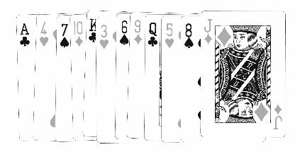
The Stebbins arrangement is easily memorized, and that’s the point. A performer who glimpses the bottom card of a cut can instantly deduce the card below it . . . which becomes the top card of the restored and squared-up deck. He can, if desired, name that card and every other card in the deck.

For the most part we are more than capable of fooling ourselves. Once you understand the hot hand illusion, you see examples of it everywhere. Many iPod users complain that the shuffle play feature isn’t random, can’t be random. It just played four Lil Wayne songs in a row! Streaks like that are to be expected. The bug isn’t in the software but in our heads.

The Manhattan bus schedule means little on busy corners, where traffic and lights cause buses to arrive in an a pproximation

to the overalternating sequences that were perceived as ran-dom. In the so-called Si Stebbins arrangement, the cards alter-nate black- red- black- red- black- red in perfect lockstep. The suits run clubs- hearts- spades- diamonds throughout the deck. The values run A-4-7-10-K-3-6-9-Q-2-5-8-J. These patterns may sound like they would stick out like a sore thumb. They don’t. The deck just looks random.



216

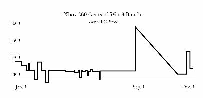
chart’s main feature is the sharp increase on September 1, fol-lowed by a decline to Black Friday. This is a not- uncommon pat-tern for holiday gift items. Retailers raise the price so that it can be lowered for holiday “sales.” The Xbox price sank to a favorable level for Black Friday and Cyber Monday, and then went abruptly up to $462. It would have been unwise to buy at that price. Bar-gain hunters shop on Black Friday and a few days afterward. Those shopping just after that are usually less price sensitive. But prices tend to revisit the Black Friday lows before Christmas, assuming the item remains in stock. Buyers and retailers are play-ing a game of chicken. Some buyers will blink and pay a high price to be sure of having an Xbox under the tree. Others will be willing to gamble and wait for the prices to come down. On December 1, Decide.com’s outguessing machine was predicting that the Xbox bundle’s price would “hold steady or drop ($133 on avg.)” over the following two weeks with 93 percent confidence. In fact, by December 4 it had dropped to $349.99.

Retail prices have become an emergent phenomenon. The retailers themselves don’t know exactly what’s going to happen next. The upward and downward jags in the chart are the result of individual sellers undercutting the competition or raising prices. These short- term price jitters are nearly impossible to


How to Outguess Home Prices

219

I’ll make that reasonable adjustment for you. I took the Case- Shiller national index and scaled it to the changing value of the dollar, using the Bureau of Labor Statistics’ Consumer Price Index. This was done so as to leave the 2000 value at 100. Here is the chart of US home values.

The first thing you’ll notice is that there was a big peak in 2006, followed by a sharp correction. This is the bubble that many homeowners (and former homeowners) are still reeling from.

The second thing you’ll observe is that the long- term return of the home market is approximately . . . zilch. Had you bought an average house in an average American community in 1987, held it for twenty- five years, and sold it in 2012, you’d be selling at just about the same price you paid, after allowing for the shrinking dollar. With broker commission and taxes, you’d lose money.

Sure, some property has appreciated in real terms. You could have bought some desert land in Nevada and found that, decades later, it’s in middle of the Las Vegas Strip. That would



228

tablecloths. They were having chicken, and the bill was $5.99. The easel had been in plain view through the show, and I was almost close enough to touch it.

Cox does what successful business forecasters do, exploit-ing an illusion of representativeness and carefully managing memories. The volunteer was neither a plant nor a random audience member. At the outset Cox announced that he wanted “a young woman,” and that’s what he got. Few women (or men) who don’t meet that description will volunteer. Sexism and ageism that wouldn’t pass in the workplace are alive on the variety act stage.

The volunteer, in her early twenties, came onstage and was shown some cards. The audience assumed that the card that Cox showed (saying ROMANCE) was typical of the cards they didn’t see. Wrong. Some of the other cards were different, offering a multiple choice of answers.

These cards cued the volunteer with possible answers for the choices she would be given. Most people are a little tongue- tied when onstage and the center of attention. They will gladly


How to Outguess the Future

229

choose one of the four canned responses. But the audience, unaware of the cards, will leave the theater wondering “What if she’d said ‘Korean barbecue food truck’?”

Another card cues the celebrity. The audience supposed the woman was choosing from the whole starry universe of celebrities. But prompted with the right four choices, most “young women” will choose Brad Pitt.

Not all the answers were cued. After the volunteer chose an Italian restaurant, Cox asked about the tablecloth and type of beverage, predicting the most likely answers ( red- and- white- checked, red wine). The questions might have been different had other restaurants been chosen. Two of Cox’s answers were wrong. This was probably the result of the volunteer’s testing Cox’s powers or forgetting a cue. Cox was prepared to get comic mileage out of his mistakes, and the goofs “proved” that he was not just making safe guesses.

The easel had multiple versions of the picture, one for each cued restaurant choice. They were gimmicked so that Cox could lift up his title card to reveal just the picture he needed.


How to Outguess the Stock Market

233

(1966), Niederhoffer and Osborne argued that stock price movements are not random at all. They described a way to out-guess the market.

Here is a chart redrawn from one in their paper. It shows a few minutes of trading in the stock of Allied Chemical. At that time, stock prices were quoted in eighths of a dollar (12½ cents).

The line in this chart doesn’t look too random, and it’s not. At upper left, the Allied Chemical price zigzags between two price points like a Ping- Pong ball. Elsewhere, it seems that traders liked the prices of $56 and $55¾, for there were streaks of trades executed at these values. Niederhoffer and Osborne proposed that a floor trader could predict these price move-ments with enough accuracy to turn a profit.

Average investors imagine that a stock has a single price fluctuating in time, like the “market price” lobster on a sum-mer resort’s menu. The reality is that there are always two prices, a bid and an ask. The bid price is the highest amount



241

won’t. Remember, that hot technology company is cannibalizing the market of older companies that are in the index, too. When you subtract the fake growth of inflation, the real, averaged- out S&P earnings don’t change much over ten years. They haven’t in the past, anyway.

The Standard & Poor’s 500 index is a fairly recent inven-tion, inaugurated in 1957. It is intended to track the 500 largest companies, by market value, publicly traded in the US stock market. Shiller backtracked and projected what 500 companies would have been in the S&P index, had it existed before 1957. He used earnings reports to reconstruct the ten- year PE back to January 1881. Here’s a chart of it.

It is hard to explain the huge variations as reasonable changes in the outlook for future earnings. Look at the rises to the big peaks in 1929 and 2000, and the equally insistent drops afterward. These were famous stock market bubbles driven by hot hand beliefs.



242

Shiller found that his backward- looking ten- year PEs have considerable power in predicting future returns. This is dem-onstrated in the chart below. Every dot represents a month, from January 1881 through January 1993. The dot’s position is determined by that month’s ten- year PE value (on the horizon-tal axis) and the return that an investor would have achieved had he invested a lump sum in the S&P 500 stocks that month and held that investment for twenty years (this return on the vertical axis). These are average annual returns over the twenty- year- period, adjusted for inflation. It’s assumed that dividends are reinvested, but this does not account for com-missions, management fees, or taxes, all of which can vary a good deal. (To save words, hereafter all quoted returns will be adjusted for inflation, and PE will mean Shiller’s ten- year PE.)

The dots are not scattered all over the chart. Instead, the dot cloud forms a diagonal swath from upper left to lower right. That means that future market returns are predictable, albeit



245

markets, investors want to do what feels good at the moment. They join the crowd and buy the stocks that are supposedly making everyone rich. The chart of one- year return doesn’t reveal a problem with that. Some buying months had positive returns even when the PE was over 40. The most obscenely overvalued markets may extend their winning streak another year. It’s only when you look at much longer periods that returns correlate with PE.

“One might have thought that it is easier to forecast into the near future than into the distant future,” Shiller wrote, “but the data contradict such intuition.” Investors, traders, and analysts are trying to predict the wrong thing: the market’s next minutes, weeks, and quarters. Most are banging their heads against a brick wall. Certainly the small investor is.

There are long regimes where investors pay scant attention to PE valuations. These periods are terminated by the mass epiphany that stocks are over- or underpriced. Once the market



250

Here’s the simplest PE-based system of all. You invest in a low- cost S&P 500 index fund, buying low and selling high (in PE terms). When the ten- year PE hits a specified high value (the sell trigger), you sell and put the proceeds in a low- cost fixed- income fund (offering the return of ten- year US Treasury bonds, let’s say). You stay in the bond fund until the PE hits a particular low value, the buy trigger. Then you buy back into the stock fund, and the cycle repeats. To make things as easy as possible, I’ll assume that you’re very busy and can check the PE — and trade when indicated — only once a month.

I tested all the plausible whole- number pairs of buy and sell limits, computing the compound return that could have been realized over the period January 1881 to January 2013. In each case the portfolio started 1881 (when the ten- year PE was 18.47) fully invested in stocks.

The table below shows the most interesting part of the results. Sell trigger values are at top, and buy trigger values are on the left. Each cell within the table gives the average real annual return, for the corresponding pair of sell and buy thresholds, over the entire 132- year period. Returns are adjusted for inflation but not for trading expenses, management fees, or taxes.



252

not-so-accurate dart thrower would be better off aiming for somewhere in the right center of the chart. Let’s say you picked 13 and 28. That would have earned a return of 6.70 percent, beating the stock market by 0.47 percentage points a year.

If that doesn’t sound like anything special, take a look at this chart. It shows the (hypothetical!) growth of a $1,000 portfolio invested since 1881. A buy- and- hold investment in the S&P stocks would have grown to an inflation- adjusted $2,932,724. A buy- low, sell- high portfolio, with PE limit values of 13 and 28, would have grown to $5,239,915.

The return is only half the story. Look at how smooth the upper line is, compared to buy- and- hold, over the past twenty years. A PE-directed investor would have sold out of stocks in January 1997, sparing herself a couple of agonizing crashes. She would have been in safe, steady fixed- income investments through January 2013. The PE investor’s superior return is due entirely to avoiding losses.



256

I’m using the same range of buy and sell values as before, and the same heat- map shading. There are more threshold pairs beating the market by 1 percent and even 1.5 percent (the darkest shading, in the center). Once again, the individual cells matter less than broad patterns. In this case, the highest returns — 14, 15, or 16 to buy and 24 or 25 to sell — form a bull’s-eye, surrounded by other high returns. A dart thrower’s reasonable aiming point might be 15/24. It returned 7.93 per-cent in this period, beating the S&P 500 by 1.70 percentage points a year.

These thresholds are less extreme than those of the sim-pler buy- low, sell- high system because you’re not necessarily trading at them. When there is momentum, the trailing limit trick can often hitch a ride. This also has the effect of produc-ing a few more trades. That helps ensure that the system will produce an advantage in the investor’s lifetime.

Let me now justify the trailing stop value of 6 percent. Here is a chart showing how returns varied with X. I’m holding 15 and 24 constant as the buy and sell triggers. All the trailing stop values through 20 percent performed respectably, though choices from 3 to 11 percent did best. Six percent had the high-est return, barely.



257

You can likewise vary the checking interval. Checking the PE just once a year — and trading if called for — would have produced a respectable return of 7.46 percent. That a monthly or yearly checking regimen performed so well may come as a shock to mobile device addicts who check the market multiple times a day. A lot can happen in a month, and that was true even in slower times. The market dropped 26 percent in October 1929. But it had dropped 11 percent the previous month. Some-one selling on a 6 percent drop would have gotten out before the crash and sold at a price about 11 percent off the peak.

Pretend an ancestor of yours started with a $1,000 US stock investment in January 1881 and that capital was completely invested with a PE momentum system ever since, using 15 and 24 as the limits. The system would have sold out of the stock market four times and bought back in four times. That’s eight trades in 132 years, or an average of about one trade every seventeen years. A typical investor can expect several trades in a lifetime.



258

Below is a chart of the ten- year PE with shaded bars mark-ing the times when a 15/24 momentum investor would have been invested in the stock market. The unshaded strips repre-sent periods when the system would have been in fixed- income investments.

Over short time frames, changes in the ten- year PE are almost all due to changes in stock prices. The chart’s steep declines in PE correspond to steep declines in stock prices. The momentum system skipped the 1929 crash and both crashes of the 2000s with remarkable timing. It sold near the top of the 1901 and 1966 bubbles, though it bought back in before the ultimate low.

Here’s a chart of portfolio value. These are real gains after allowing for the diminishing dollar (but not transaction costs, management fees, and taxes). During this 132- year period an



259

investment in ten- year US Treasury bonds might have turned an initial $1,000 into $18,704, inflation adjusted. I do not chart that because the line would hug the axis so closely as to be indistinguishable from it.

A buy- and- hold stock investor in the S&P 500 and its precur-sor companies would have turned $1,000 into about $2,932,653. An investor using the PE momentum system to switch between stocks and bonds would have realized $23,836,362. That’s over 8 times the wealth of a buy- and- hold investor.

Nobody invests for 132 years. Let’s look at something a little easier to relate to, the twenty years from January 1993 to January 2013. This time we start with $1,000 in 1993. A bond investment would have grown to $1,617 in real terms. A buy- and- hold stock investment would have risen to $3,173. The PE momentum system would have ended up with $5,517.



260

It would have done that by making just two trades. The buy- and- hold portfolio was ahead of the momentum system for brief periods at the peaks of the dot- com and subprime mortgage bub-bles. It didn’t stay ahead for long, though, and it didn’t finish ahead. The buy- and- holder weathered two horrific declines. In the first, the stock portfolio lost 43 percent of its value. In the second, it lost 50 percent. (These figures may be different from what you’ve heard, as they account for reinvested dividends and inflation.)

At the bottom of the market’s second plunge, in March 2009, the stock portfolio’s value was nearly tied with that of the bond portfolio. That’s one demonstration that stocks do not always outperform bonds over fairly long periods.

The dotted line labeled “Capitulator” represents the pos-sible fate of someone who considered himself a buy- and- hold investor but who was spooked by the second big plunge in a decade. Exasperated by weeks of declines, the capitulator threw in the towel. He sold, vowing never to invest in stocks again.


rock breaks scissors - reference guide

Documents

hidden watch

watch isnt

volunteer supplies

performer lifts cup

audience volunteer

nationwide test of esp

mentalists powers

amrock breaks scissors52