rivm rapport 711701049 site-specific human risk assessment
TRANSCRIPT
Site-specific human risk assessment of soil contamination with volatile compounds
Report 711701049/2008J. Bakker | J.P.A. Lijzen | H.J. van Wijnen
RIVM, P.O. Box 1, 3720 BA Bilthoven, tel.: 31 - 30 - 274 91 11; fax.: 31 - 30 - 274 29 71, www.rivm.nl
RIVM Rapport 711701049/2008
Site-specific human risk assessment of soil contamination with volatile compounds
J. Bakker J.P.A. Lijzen H.J. van Wijnen Contact: J. Bakker RIVM-Stoffen Expertise Centrum [email protected]
This investigation has been performed by account of the Ministry of Spatial Planning, Housing and the Environment, Directorate General for the Environment, Directorate of Sustainable Production (DGM-DP), within the framework of project 711701, Risks in relation to Soil Quality

2 RIVM report 711701049
© RIVM 2008 Delen uit deze publicatie mogen worden overgenomen op voorwaarde van bronvermelding: 'Rijksinstituut voor Volksgezondheid en Milieu (RIVM), de titel van de publicatie en het jaar van uitgave'.
RIVM report 711701049 3
Het rapport in het kort
Locatiespecifieke humane risicobeoordeling van bodemverontreiniging met vluchtige verbindingen Het RIVM heeft het zogeheten VOLASOIL-model verbeterd. Het model schat voor woningen en andere gebouwen de binnenluchtconcentraties die ontstaan als gevolg van bodemverontreiniging met vluchtige verbindingen. Deze verontreiniging van bodem en grondwater kan zich voordoen in de omgeving van bijvoorbeeld benzinestations en chemische wasserijen. Om de risico’s hiervan voor de mens te kunnen bepalen, berekent het model op basis van de vervuilingsgraad van het grondwater de concentraties vluchtige stoffen in de binnenlucht. Het aangepaste model maakt een betere risicobeoordeling mogelijk, zodat de mate van spoed om te saneren beter is te bepalen. De nieuwe versie is voor meer typen woningen bruikbaar, namelijk voor woningen zonder kruipruimte of woningen met een kelder. Eerder was het alleen bruikbaar voor woningen met een kruipruimte. Als vergelijking zijn voor de toegevoegde woningtypen twee alternatieve berekeningsmethoden opgenomen die internationaal worden toegepast. Het rapport onderbouwt bovendien de waarden voor de belangrijkste parameters van de modelconcepten. Onder andere zijn karakteristieke eigenschappen van zes standaard bodemtypen vereenvoudigd en verduidelijkt, waardoor lokale beoordelingen beter zijn uit te voeren. Daarnaast is aangeven wat de belangrijkste locatiespecifieke gegevens zijn van het model. Het is de bedoeling de modelconcepten van de nieuwe VOLASOIL-versie te gebruiken bij het beleidsinstrument voor bodemsanering (SANSCRIT), de uitwerking van het in 2008 herziene Saneringscriterium bodemsanering. Op basis van de resultaten van de modelberekeningen kan besloten worden aanvullende (binnen)luchtmetingen te doen. De combinatie van modelleren en meten geeft de beste basis om de risico’s van vluchtige verbindingen voor de mens te beoordelen. Trefwoorden: VOLASOIL, bodemverontreiniging, binnenlucht, vervluchtiging
4 RIVM report 711701049
Abstract
Site-specific human risk assessment of soil contamination with volatile compounds RIVM has improved the VOLASOIL model. The model estimates the indoor air concentration of houses and other buildings originating from soil contamination with volatile compounds. This contamination occurs for example in the vicinity of petrol stations and dry cleaning. To estimate the risks for humans, the model calculates the air concentrations based on the concentrations in soil and or groundwater. The extended and updated model facilitates a better risk assessment in the process of determination of the urgency for remediation. In the past, the model only was suitable for buildings with a crawlspace. The current version is extended for slab-on-grade buildings and buildings with a basement. For comparison with the standard modelling approach concept also two alternative model concepts are included, which have been applied in other international models. These alternative calculation models should only be used by expert users. Furthermore the background and underpinning of the most relevant parameters has been evaluated and has led to an adjustment of the values that can be selected in a site specific risk assessment. Also the most important site specific parameters are given in the report. The scenarios and model concepts in VOLASOIL can be applied in the Remediation Criteria (SANSCRIT), being revised in 2008. Based on the results of these model calculations it can be decided whether unacceptable risks can be excluded. If not, it can be decided to do additional (indoor) air measurements. The combination of modelling and air measurements gives the best basis for decisions about human health risks and about the urgency for remediation. Key words: VOLASOIL, soil contamination, indoor air pollution, vapour intrusion
RIVM report 711701049 5
Preface
This research at the National Institute for Public Health and the Environment (RIVM) has been carried out by commission of the Ministry of Housing, Spatial Planning and the Environment (VROM), Directorate General for the Environment, Directorate of Sustainable Production (DGM-DP). The subject of the risk assessment of volatile compounds, including the modelling, has been extensively discussed with an external advisory group composed of a number of experts from several institutes, consultancies and competent authorities. Members of this group were: A. Mayer (Mayer Milieuadvies), J. Tuinstra (Royal Haskoning, now TCB), J. Schreuder (DHV), J. Provoost (VITO, B), J. ter Meer (TNO) and M. Waitz (Ingenieursbureau Amsterdam). We are also very grateful for the information, advice and remarks provided by the ‘expert group on human-toxicological risk assessment’ (S. Boekhold (TCB), C.J.M. van de Bogaard (VROM-Inspectie), D.H.J. van de Weerdt (HGM Arnhem), T. Fast (Fastadvies), C. Hegger (GGD Rotterdam), J.E. Groenenberg (Alterra), J. Wezenbeek (Grontmij), J. Tuinstra (TCB), R.M.C. Theelen (Ministerie van LNV), S. Dogger (Gezondheidsraad), Th. Vermeire (RIVM) and J. Lijzen (RIVM). Currently the new VOLASOIL model is programmed in excel, combined with the human exposure model CSOIL. It is planned to develop an external version that can be approached or downloaded from the internet. Both this report and model code have been produced with care, however, these products cannot be claimed to be free of errors. Use of the results obtained by means of these materials is for the full responsibility of the user. Use of the model is encouraged and feedback is welcomed. However, other than by means of this report, no technical support is being offered.

6 RIVM report 711701049
RIVM report 711701049 7
Contents
Samenvatting 10
Summary 11
1. Introduction 13
1.1 Background 13 1.2 Validation study 14 1.3 External recommendations and evaluations 15 1.4 Readers guide 15
2. Framework for site-specific human risk assessment 17
2.1 General framework 17 2.2 Measurements of (indoor) air concentrations 20
3. Modelling of exposure to indoor air 23
3.1 Introduction 23 3.2 Building and contamination scenarios 23
3.2.1 Building scenarios 23 3.2.2 Contamination scenarios 26
3.3 Input parameters 27 3.4 Exposure scenarios and exposure assessment 27 3.5 Other (international) model concepts for indoor air modelling 28
3.5.1 Ground bearing slab, model concept and assumptions 28 3.5.2 House with basement, crack at wall-floor interface, model concepts and assumptions 31 3.5.3 House with crawl space 34 3.5.4 General discussion on model concepts 37
4. Model concepts for different types of buildings 39
4.1 Introduction 39 4.2 Building with crawlspace 39
4.2.1 Transport from soil/groundwater to the crawlspace 39 4.2.2 Calculation of indoor air concentration, scenario crawlspace 42
4.3 Slab-on-grade building 43 4.3.1 Construction types 43 4.3.2 Combined diffusive and convective transport for two layers, the soil-floor system 43 4.3.3 Calculation of the diffusive flux through the soil-floor column 47 4.3.4 Calculation of the convective air flux through the soil-floor column 47 4.3.5 Calculation of indoor air concentration, scenario slab-on-grade 50
8 RIVM report 711701049
4.4 Building with basement 51 4.4.1 General assumptions 51 4.4.2 Contaminant transport into the cellar, basic calculations 51 4.4.3 Calculation of indoor air concentration, scenario slab-on-grade 53
4.5 Contaminant scenarios 54 4.5.1 Groundwater contamination; well-mixed container 54 4.5.2 Contaminated groundwater in crawl space or basement 54 4.5.3 Floating soil-contaminant layer in the open capillary zone 55 4.5.4 Groundwater in crawl space or basement and a floating soil-contaminant layer 55 4.5.5 Pure contaminant in open capillary zone 55 4.5.6 Very low groundwater table 56 4.5.7 Sinking soil-contaminant layer 56 4.5.8 Contaminant source beneath the groundwater table 56 4.5.9 Estimating the vapour concentration of mixtures 56
4.6 Estimating source depletion 58
5. Selection of input parameters 59
5.1 General 59 5.2 Physicochemical and toxicological data 59 5.3 Site specific data 60 5.4 Other site specific data 60
5.4.1 Soil type 61 5.4.2 Air permeability soil 61 5.4.3 Height capillary transition boundary 63 5.4.4 Quality of the floor 66 5.4.5 Permeability and porosity of the floor and other building elements 67 5.4.6 Perimeter seam gap and crack ratio 71 5.4.7 Ventilation characteristics, living room 71 5.4.8 Ventilation characteristics crawl space 72
5.5 Generic input parameters 73 5.5.1 Air pressure difference 73 5.5.2 Dimensions of the building, crawl space and cellar 75 5.5.3 Floor and wall thickness 76
5.6 Overview parameters and default values 76
6. Uncertainty and sensitivity analysis 81
6.1 Introduction 81 6.2 Methods 81
6.2.1 Scenario analysis 81 6.2.2 Generic approach 81
6.3 Results 84 6.3.1 Sensitivity analysis 84 6.3.2 Uncertainty analysis 88
6.4 Conclusion 92
7. Conclusions and recommendations 93
RIVM report 711701049 9
References 95
Appendix 1 Derivation of combined diffusive and convective transport through two layers, intact concrete floor 101
Appendix 2 Derivation of combined diffusive and convective transport through two layers, floor with cracks and gaps or a perimeter seam gap 105
Appendix 3 Combined diffusive and convective transport for contaminant source beneath the groundwater table 109
Appendix 4 Overview of chronic limit values (TCA) 112
Appendix 5 Temperature correction of the vapour pressure and solubility 115
Appendix 6 Additional substance properties 117
Appendix 7 Example calculations for slab-on-grade and basement building scenarios 118 7.1 Slab-on-grade, intact floor 118 7.2 Slab-on-grade, perimeter seam gap 120 7.3 Slab-on-grade, floor with gaps and holes 122 7.4 Basement, intact floor and walls 124
Appendix 8 Dutch soil texture terminology 128
Appendix 9 Model input-parameter distributions 129
Appendix 10 Results of the Uncertainty analyses for the VOLASOIL approach 133
Appendix 11 Results of the Uncertainty analyses for the Johnson and Ettinger approach 137
10 RIVM report 711701049
Samenvatting Voor het schatten van de mate van bodemverontreiniging en de mogelijke effecten hiervan op de mens wordt gebruikgemaakt van het VOLASOIL-model. Het VOLASOIL-model berekent de concentratie in de binnenlucht van een woning die gebouwd is op een bodem die verontreinigd is met vluchtige verbindingen. Omdat het VOLASOIL-model alleen bruikbaar was voor woningen met een kruipruimte en er naast dit type eveneens woningen zijn met een kelder of woningen zonder kruipruimte, was er vanuit de praktijk van de risicobeoordeling de wens het model uit te breiden. Literatuuronderzoek wees uit dat er een aantal verschillende modellen is voor deze twee typen gebouwen en dat het transport vanuit de bodem naar de binnenlucht van een woning op een aantal verschillende manieren kan worden berekend. Uit het oogpunt van consistentie is er voor gekozen om zoveel mogelijk bij het bestaande model voor de woning met een kruipruimte aan te sluiten. Voor de berekening van de concentraties in de binnenlucht voor de twee nieuwe modellen zijn eveneens twee alternatieve berekeningsmethoden opgenomen. Deze alternatieve berekeningsmethoden worden gebruikt in internationaal bekende alternatieve schattingsmodellen. De alternatieve rekenmodellen zijn niet bedoeld voor de standaard locatiespecifieke risicobeoordeling maar zijn bedoeld voor het uitvoeren van aanvullende beoordelingen door experts ter vergelijking met de standaardmethode. Naast het opstellen van modelconcepten voor de twee alternatieve woningtypen, is er uitgebreid literatuuronderzoek gedaan naar de waarde van de parameters die in de berekeningen worden gebruikt. Het gaat onder meer om de locatiespecifieke parameters, zoals porositeit en luchtdoorlatendheid per bodemtype, de kwaliteit van de vloer en de ventilatiekarakteristieken, en de generieke parameters zoals drukverschillen in de bodem en tussen bodem en huis. Uit de verzamelde gegevens zijn de meest gangbare standaardwaarden afgeleid en is een aantal waarden aangepast. Ook is in het rapport aangeven hoe de verschillende waarden voor verschillende situaties in de praktijk toe te passen. Het rapport bevat eveneens een gevoeligheids- en onzekerheidsanalyse. Met deze analyses is geprobeerd inzicht te verkrijgen in het gedrag van de drie verschillende modellen. De analyses geven daarnaast aan wat de belangrijkste parameters zijn van het model. Hierop kan men zich vervolgens richten om indien noodzakelijk een betere schatting te maken van de concentraties in de binnenlucht van woningen. Het is de bedoeling dat de modelconcepten voor de twee nieuwe woningtypen in VOLASOIL toegepast gaan worden in het nieuwe Saneringscriterium. Op basis van de resultaten van deze modelberekeningen kunnen luchtmetingen worden gedaan. Berekeningen en metingen samen geven de beste basis voor het bepalen van risisco’s van vluchtige verontreinigingen.
RIVM report 711701049 11
Summary The human risk assessment of soil contamination with volatile compounds can be based on modelling the indoor air concentration and measurement of the air concentrations. For the modelling of the indoor air concentration the VOLASOIL model can be used. This report presents the results of the update of the model and describes the principle of site-specific risk assessment of soil contamination with volatile compounds. Previously, the VOLASOIL model could be used only for buildings with a crawlspace (below the living floor). The new model is extended with a scenario for buildings with a basement (cellar) and a scenario for slab-on-grade buildings, because of the existence of these other types of dwellings and the expressed desire of model users. The literature search carried out showed that different model concepts are available for these additional building scenarios and that the transport from the soil to the indoor air can be calculated in alternative ways. For the additional building scenarios one default and two alternative model concepts have been included. The alternative concepts are being used in internationally known exposure estimation models. Literature research was carried out for the most relevant model parameters. This concerns site specific parameters, like soil type dependent porosity and air permeability, the quality of the floor and ventilation characteristics, and general parameters like pressure differences in the soil and between soil and buildings. The values were evaluated and the best values for site specific risk assessment were selected, leading to an adjustment of the values that can be selected in site specific risk assessment. It is also indicated, which values can be used in different situations. A sensitivity and uncertainty analysis was carried out with each model concepts applying common value ranges for the relevant parameters. The results indicate how the models perform in different situations and show which parameters are the most important depending on the circumstances. This information is important when the model is used to estimate the indoor air concentrations and to carry out a risk assessment for volatile compounds originating from soil contamination. The scenarios and model concepts for the two new building types in VOLASOIL can be applied in the Remediation criterion, which is being revised in 2008. Based on the results of these model calculations it can be decided whether unacceptable risks can be excluded or not. If not, it can be decided to remediate or to do additional air measurements. The combination of modelling and measurements gives the best bases for decisions about human health risks.

12 RIVM report 711701049
RIVM report 711701049 13
1. Introduction
1.1 Background Risk assessment of human exposure to volatile compounds in soil and groundwater has been part of the assessment of soil contamination for a long time in the Netherlands. It is included in de human exposure model CSOIL that is used for deriving of the Intervention Values for soil and groundwater (Swartjes, 1999; Lijzen et al., 2001). The current Intervention Values are given in a Ministerial Circular (VROM, 2000). The estimation of the exposure to volatile compounds for generic risk assessment is based on a standard residential scenario with fixed building dimensions and soil conditions. With these settings, generic risk limits (Intervention Values) for soil and groundwater can be derived. For site specific risk assessment it has been made possible to adjust the most relevant parameters to estimate the concentration in indoor air based on the measured concentrations in soil and groundwater. First, for site specific risk assessment in general the Remediation Urgency Method (RUM) was developed (in Dutch: Saneringsurgentie systematiek’: SUS (VROM, 1995)). The site specific risk assessment in SUS helps to determine the urgency for remediation and supports decisions about how to remediate contaminated sites. The SUS consists of three elements: o human risks; o ecological risks; o risk due to contaminant migration. A site with soil contamination is not considered to be urgent when there is no actual risk for one of these elements. To support the risk assessment of volatile compounds in particular the VOLASOIL model was developed (Waitz et al., 1996). This model gave more opportunities to adjust to the local situation and included also a modification of the model concept. The VOLASOIL model calculates the indoor air concentration for the Dutch situation in buildings situated on soils contaminated with volatile compounds. The model is suitable for site-specific risk assessment because of the possibility of a flexible combination of modelling and measurements. It can be used for several specific contamination cases, for instance floating contaminant layers, contaminant sources beneath the groundwater table, pure contaminant in the open capillary zone, contaminated groundwater in crawl spaces, et cetera. The starting point for the improvement is the current remediation urgency method (RUM), as described in VROM (1995), together with the concepts in the VOLASOIL model and the results of the evaluation of the intervention values. The goal of this study was to improve the site specific human risk assessment of soil and groundwater contamination. Recently an extended political evaluation of the framework for soil quality assessment was published (VROM, 2003a). This resulted in a revised philosophy on soil protection. The main additions to the present philosophy concern: o a simpler and more consistent framework; o more focus on sustainability; o a (further) shift to fitness for use and regional responsibility. In 2006 a Ministerial Circular on soil remediation was published (VROM, 2006) that replaces the Remediation Urgency Method. In particular the policy has changed whereas the risk assessment methodology is still almost the same. The use of measurements in contact media has gained importance in the second step of the risk assessment. In 2008 also the Ministerial Circulair was updated with the calculation of site specific risks, including information presented in this report. This Circular and the new soil policy include a (further) shift to fitness for use. This means that site-specific risk assessment will gain importance. The approach presented in this report is part of a revised methodology on site specific human risk assessment (Lijzen et al., in prep.).
14 RIVM report 711701049
Based on the analysis presented in Lijzen et al. (2003) objectives were defined for further improvement of the site-specific risk assessment. Based on interviews with experts and earlier evaluations of the method, the main restraints are indicated and options for solutions have been prioritised, partly based on scientific feasibility. It was planned to focus on separate parts of the methodology. Besides the general human risk assessment, the emphasis lay on the following restraints related tot the human exposure to soil contamination with volatile compounds: o uncertainty about the determination of the human risks for inhalation of indoor air; o lacking of the determination of the risk of volatile compounds in buildings with a slab-on-grade floor; o weighing of results from model calculations with measurements; o lacking of pragmatic guidelines for additional measurements (bioavailability, indoor air, consumption
crops). The following subjects were identified to improve the risk assessment and help to solve these restraints: o evaluation of guidelines for measurements of contaminants in (indoor) air in relation to soil pollution and
the relation between calculations and measurements; o implementation of the results of the project Evaluation of Intervention Values soil (Lijzen et al., 2001); o development of a model concept for the risk assessment of volatile compounds in buildings without a
crawlspace (slab-on-grade); o integration of the exposure models VOLASOIL and CSOIL; o discussion on how modelling and measurements should be integrated in a framework (also based on the
expected uncertainties within both methods). Existing field data of volatile compounds in indoor air have been used to carry out a validation study (Van Wijnen and Lijzen 2006; see section 1.2). For the transport of volatile compounds into buildings also additional model development has been carried out, which is presented in this report. For performing measurements in (indoor) air, a guideline is written that gives guidance on how to carry out measurements and how to interpret in relation with calculations (Otte et al., 2007).
1.2 Validation study In 2004 and 2005 a validation study (Van Wijnen and Lijzen, 2006) was carried out in order to compare risk assessment based on modelling with actual measurements in soil air, crawlspace and basement air, and indoor air. In that report it was concluded that the VOLASOIL model estimates the indoor air concentrations for tetrachloroethylene and trichloroethylene reasonably well. The study shows that the model overestimates at high groundwater concentrations and underestimates at lower groundwater concentrations. This does not have to be a problem when it is accepted that some overestimation is functional, because the estimation should be protective for most situations. In a second step, measurements can reduce the potential overestimation. To establish a realistic air concentration (with a higher probability of underestimations) a revision of the current model is needed. Some factors can be important in explaining the differences between modelling and actual measurements: e.g. degradation in the unsaturated zone; limits in the transport from contaminants from groundwater to the soil air; the type of building and the season in which measurements are carried out. In the report the following recommendations were given for adjustment of the modelling of indoor air concentrations: o Adjustment of the relationship between crawlspace air and indoor air is necessary in the way that the
default contribution of crawlspace air to indoor air is between 0.1 and 0.3 (current default value of 0.1 is lower);
o Adjustment of the transport from groundwater to crawlspace air. The transport could be systematically lowered, but when worst case calculations are acceptable no adjustments should be made;
RIVM report 711701049 15
o For risk assessment only groundwater concentrations under or within 10 meters of the building and concentrations in the top layer of the groundwater should be used;
o There should be a guideline on how to deal with heterogeneity of the contamination and the time scale in which groundwater measurements can be used for risk assessment;
o More information should be given on the distribution of input-parameters in order to make an easier selection;
o The soil air fraction should be soil type dependent; o A mass balance check should be added to be able to check how long a calculated flux can exist; o It should be possible to use the depth of the unsaturated zone instead of the depth of the groundwater
table. These recommendations are used in the further development of the existing model.
1.3 External recommendations and evaluations In advises of the Soil Technical Committee (TCB, 2002) and the Dutch Health Council (Health Council, 2004) about deriving Intervention values (generic Soil Quality criteria) it was stated that modelling of air concentrations implies a lot of uncertainty and that site specific measurements should be important in making decisions about remediation. Also it was stated that the model concept of volatilisation was not validated. Part of the uncertainty can be reduced by using site-specific information in the risk assessment. Secondly the risk assessment can be improved by carrying out measurements in contact media or somewhere in the transport route from source to receptor. Discussing these subjects brings us to the question to what extent modelling should contribute to the risk assessment of volatile compounds. In principle modelling and measurements should not lead to complete different assessment of risks and both should support each other in a methodology. Modelling gives results that can be reproduced, whereas measurements in air are more relevant for the actual exposure, but can be (extremely) time dependant. For the site specific risk assessment it was therefore decided that site specific modelling should be the start of risk assessment and that measurements should be used in the next step of a tiered procedure in the case that the objectives are exceeded. For more details about this procedure we refer to chapter 2.
1.4 Readers guide In chapter 2 a revised framework for site-specific human-toxicological risk assessment is presented and the relation with the Ministerial Circular on soil remediation criteria is given. Also an outline of the possibilities to carry out measurements in air is given in chapter 2. Chapter 3 describes the situations and contamination scenarios that should be identified when modelling the indoor air concentration. Chapter 4 describes the model concepts of indoor air modelling of volatile compounds for different building types and contamination scenarios. In chapter 5 the most important model parameters are described and the advised default settings and choices are given. In chapter 6 a sensitivity and uncertainty analysis was carried out. The conclusions and recommendations are summarised in chapter 7.

16 RIVM report 711701049
RIVM report 711701049 17
2. Framework for site-specific human risk assessment
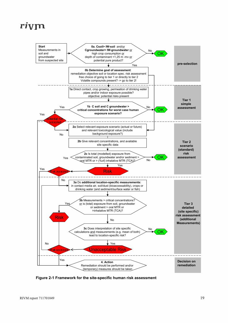
2.1 General framework Until recently the method for the site-specific human risk assessment was put down in the Remediation Urgency Method (SUS) (VROM, 1995, 1998). This method was implemented in a computerised decision support system. This computer software was developed by the Van Hall Institute by order of the Ministry of VROM in 1995. The new Dutch soil policy (‘Beleidsbrief bodem’: VROM, 2003a) includes, amongst others, a (further) shift to fitness for use. This means that the site specific risk assessment will gain importance. In 2006 the Remediation Urgency System is replaced by a new Remediation Criteria (in Dutch: Saneringscriterium) in the Ministerial Circular on soil remediation 2006. The Remediation Criteria is therefore the policy context of the framework, being updated in 2008 (VROM, 2006, 2008). To improve the location specific (or actual) risk assessment several activities have been carried out. This included the framework of the human site specific risk assessment. This framework and its elements will be reported more extensively (Lijzen et al., in prep). It supports the approach as presented in the published Remediation Criteria (VROM, 2006, 2008). The framework should be suitable for different goals: o determination of the urgency for remediation of contaminated sites; o advise local authorities about health risks for humans; o deriving remediation objectives and soil quality standards. In Figure 2-1 the scheme of the framework is given. The different steps in the framework are shortly described with a focus on the assessment of volatile compounds. Within the framework a tiered approach is chosen, comparable with the approach that is currently used in the remediation urgency method. As indicated, the result of the assessment should primarily be used in setting the environmental priority for remediation, but can also be used for setting standards for land use specific soil quality. Figure 2-1 presents the three tiers of the framework and the preselection. Preselection In the preselection phase it should be made clear which measured concentrations should be used for the risk assessment. When these concentrations are higher than a certain level (Intervention Values) tier 1 should be started. Other specific circumstances could also be described in which risk assessment is necessary, besides concentration levels. For example when volatile compounds are found in groundwater and the groundwater level is very shallow. Furthermore the goal of the risk assessment has to be set in this tier, because this influences the selected toxicological criteria. For volatile compounds e.g. the goal can be to know if the indoor air is influenced by contamination in soil and groundwater. In that case not only the Tolerable Concentration in Air (TCA) is used for the assessment. Tier 1 For tier 1 it is proposed to make clear -with a concentration list- below which concentrations in soil and groundwater no human risks are expected (below the Maximum Tolerable Risk level, MTR, for humans). Therefore the relevant exposure pathways are determined (ingestion of and dermal contact with soil and dust, crop consumption, inhalation of indoor air, permeation of drinking water mains and fish consumption). In fact worst case situations are being calculated. For volatile compounds it is recommended to go to tier 2 directly, because location specific information can be used for the assessment (depth of groundwater table, type of soil
18 RIVM report 711701049
and type of building). In case that a floating layer or pure product is present in unsaturated soil, you should go to tier 2 and tier 3. In the circumstance that it is already decided to remediate, sometimes additional human risk assessment is not carried out. In these cases it can be concluded, based on this information, whether a potential risk for humans is present or not. Tier 2 In tier 2 a more extensive risk assessment is carried out, based on specific standard scenarios, measured concentrations and site-specific data. Only standard site-specific data that can easily be measured are used. This tier can be used in the standard risk assessment of the Remediation Criteria (VROM, 2006). When the Maximal Permissible Risk (or Negligible risk) is exceeded based on this assessment, a tier 3 risk assessment should be carried out ór the risk should be accepted and measures/remediation should be carried out to reduce the risks for humans. This report focuses on the model concepts that can be implemented for exposure assessment in this tier. Tier 3 In tier 3 more site specific information can be used. Especially measurements in contact media can carried out, but also other measurement to improve the risk assessment can be done. In particular the following media could be measured: o concentrations in air (indoor air, crawlspace air, and basements, soil air and/or outdoor air); o concentrations in plants (or measurement of bioavailability in soil related to the plant content); o bioaccessibility of contaminants in soil/dust within the gastro-intestinal track (in particular for lead and
arsenic); o concentrations in drinking water; o concentrations in fish. For the sampling of these media a uniform guideline or protocol is necessary. Guidelines for the first three types of measurements are published in Otte et al. (2007), Swartjes et al. (2007) and Oomen et al. (2006). In these guidelines it should be made clear when and how measurements can be carried out and how the results of the additional research should be interpreted compared to the calculations. These guidelines will have a position in Remediation Criteria method and have been tuned with important stakeholders. A summary of the guideline for indoor air measurements is given in section 2.2. Decision of local authority The general framework ends with a decision or action (tier 4). In the context of the Remediation Criteria (‘Saneringscriterium’) it is stated that unacceptable risks should be eliminated as soon as possible (temporary measures to reduce exposure) and that, in principle, remediation should start within 4 years after the decision of the authority.
RIVM report 711701049 19
Yes
Tier 1simple
assessment
pre-selection
No
Tier 2scenario
(standard) risk
assessment
2a Select relevant exposure scenario (actual or future) and relevant toxicological value (include
background exposure?)
2b Give relevant concentrations, and available site specific data
Yes
Tier 3detailed
(site specific)risk assessment
(additional Measurements)
NoYes
3a Do additional location-specific measurements:in contact media air, soil/dust (bioaccessability), crops or
drinking water (and sediment/surface water or fish)
Risk accepted
OK
OK
No
No
OK
Yes
Risk accepted
Risk
No
No
Unacceptable Risk
4. ActionRemediation should be performed and/or
(temporary) measures should be taken
Decision onremediation
potential riskaccepted
NoOK
1a Direct contact, crop growing, permeation of drinking water pipes and/or indoor exposure possible?
objective: potential risks present
0b Determine goal of assessment: remediation objective soil or location spec. risk assessment
free choice of going to tier 1 or directly to tier 2Volatile compounds present? -> go to tier 2!
Yes
0a. Csoil> IW-soil and/orCgroundwater> IW-groundwater or
high crop consumption ordepth of contaminant <1,25 m -mv or
potential pure product?
1b C soil and C groundwater > critical concentrations for worst case human
exposure scenario?
Yes
Yes
2c Is total (modelled) exposure from contaminated soil, groundwater and/or sediment >
oral MTR or > (%of) inhalative MTR (TCA)?
3c Does interpretation of site specific calculations and measurements (e.g. mean of both)
lead to location-specific risk?
3b Measurements > critical concentrations? or is (total) exposure from soil, groundwater
or sediment > oral MTR or >inhalative MTR (TCA)?
StartMeasurements in soil and groundwaterfrom suspected site
No
Yes
RiskYes
Figure 2-1 Framework for the site-specific human risk assessment
20 RIVM report 711701049
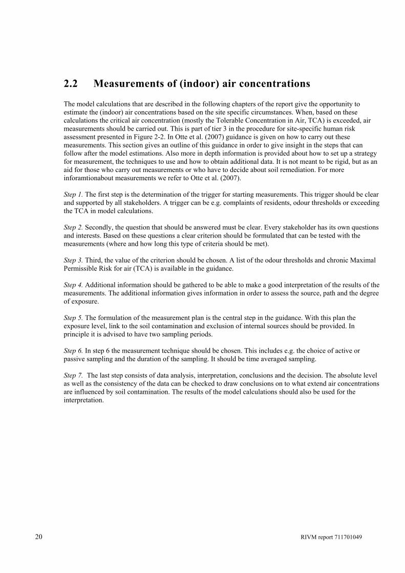
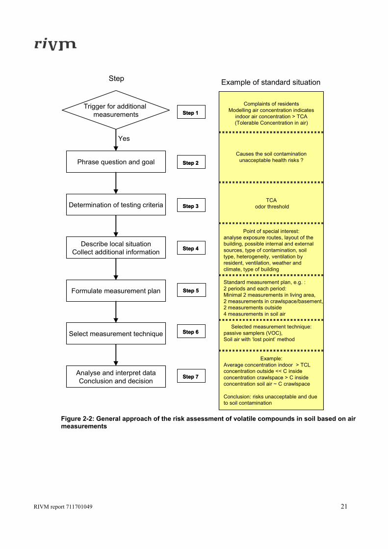
2.2 Measurements of (indoor) air concentrations The model calculations that are described in the following chapters of the report give the opportunity to estimate the (indoor) air concentrations based on the site specific circumstances. When, based on these calculations the critical air concentration (mostly the Tolerable Concentration in Air, TCA) is exceeded, air measurements should be carried out. This is part of tier 3 in the procedure for site-specific human risk assessment presented in Figure 2-2. In Otte et al. (2007) guidance is given on how to carry out these measurements. This section gives an outline of this guidance in order to give insight in the steps that can follow after the model estimations. Also more in depth information is provided about how to set up a strategy for measurement, the techniques to use and how to obtain additional data. It is not meant to be rigid, but as an aid for those who carry out measurements or who have to decide about soil remediation. For more inforamtionabout measurements we refer to Otte et al. (2007). Step 1. The first step is the determination of the trigger for starting measurements. This trigger should be clear and supported by all stakeholders. A trigger can be e.g. complaints of residents, odour thresholds or exceeding the TCA in model calculations. Step 2. Secondly, the question that should be answered must be clear. Every stakeholder has its own questions and interests. Based on these questions a clear criterion should be formulated that can be tested with the measurements (where and how long this type of criteria should be met). Step 3. Third, the value of the criterion should be chosen. A list of the odour thresholds and chronic Maximal Permissible Risk for air (TCA) is available in the guidance. Step 4. Additional information should be gathered to be able to make a good interpretation of the results of the measurements. The additional information gives information in order to assess the source, path and the degree of exposure. Step 5. The formulation of the measurement plan is the central step in the guidance. With this plan the exposure level, link to the soil contamination and exclusion of internal sources should be provided. In principle it is advised to have two sampling periods. Step 6. In step 6 the measurement technique should be chosen. This includes e.g. the choice of active or passive sampling and the duration of the sampling. It should be time averaged sampling. Step 7. The last step consists of data analysis, interpretation, conclusions and the decision. The absolute level as well as the consistency of the data can be checked to draw conclusions on to what extend air concentrations are influenced by soil contamination. The results of the model calculations should also be used for the interpretation.
RIVM report 711701049 21
Yes
Step 1Step 1
Step 4 Step 4
Step 5Step 5
Step 2Step 2
Step 3Step 3
Step 6 Step 6
Step 7Step 7
Complaints of residentsModelling air concentration indicates
indoor air concentration > TCA (Tolerable Concentration in air)
Causes the soil contamination unacceptable health risks ?
TCAodor threshold
Point of special interest:analyse exposure routes, layout of the building, possible internal and external sources, type of contamination, soil type, heterogeneity, ventilation by resident, ventilation, weather and climate, type of building
Standard measurement plan, e.g. :2 periods and each period:Minimal 2 measurements in living area, 2 measurements in crawlspace/basement,2 measurements outside4 measurements in soil air
Selected measurement technique:passive samplers (VOC),Soil air with ‘lost point’ method
Example:Average concentration indoor > TCLconcentration outside << C inside concentration crawlspace > C insideconcentration soil air ~ C crawlspace
Conclusion: risks unacceptable and due to soil contamination
Example of standard situationStep
Phrase question and goal
Determination of testing criteria
Formulate measurement plan
Describe local situationCollect additional information
Select measurement technique
Analyse and interpret dataConclusion and decision
Trigger for additional measurements
Figure 2-2: General approach of the risk assessment of volatile compounds in soil based on air measurements

22 RIVM report 711701049
RIVM report 711701049 23
3. Modelling of exposure to indoor air
3.1 Introduction When volatile compounds are present in soil or groundwater above Intervention Values it is recommended to carry out calculations to estimate the indoor air concentration based on site specific characteristics. It should also be noticed that below the (human) Intervention Value risks could occur in case the groundwater is very shallow or the contamination is within the first meter of the soil. This recommendation means that worst case calculations, as suggested for tier 1 of the framework, are not recommended for volatile compounds. In this chapter the general setup of the modelling is described. Before calculations can be done, the appropriate scenario should be chosen that fits the type of building and type of contamination (see section 3.2). Some general aspects of the input parameters are mentioned in section 3.3. In section 3.4 the relation with the exposure scenarios is described. An exploration of the internationally available model concepts is presented in section 3.5.
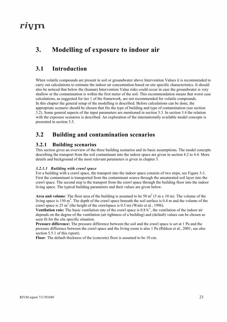
3.2 Building and contamination scenarios 3.2.1 Building scenarios This section gives an overview of the three building scenarios and its basic assumptions. The model concepts describing the transport from the soil contaminant into the indoor space are given in section 4.2 to 4.4. More details and background of the most relevant parameters is given in chapter 5. 3.2.1.1 Building with crawl space For a building with a crawl space, the transport into the indoor space consists of two steps, see Figure 3-1. First the contaminant is transported from the contaminant source through the unsaturated soil layer into the crawl space. The second step is the transport from the crawl space through the building floor into the indoor living space. The typical building parameters and their values are given below. Area and volume: The floor area of the building is assumed to be 50 m2 (5 m x 10 m). The volume of the living space is 150 m3. The depth of the crawl space beneath the soil surface is 0.4 m and the volume of the crawl space is 25 m3 (the height of the crawlspace is 0.5 m) (Waitz et al., 1996). Ventilation rate: The basic ventilation rate of the crawl space is 0.8 h-1, the ventilation of the indoor air depends on the degree of the ventilation (air tightness of a building) and (default) values can be chosen as seen fit for the site specific situation. Pressure difference: The pressure difference between the soil and the crawl space is set at 1 Pa and the pressure difference between the crawl space and the living room is also 1 Pa (Rikken et al., 2001; see also section 5.5.1 of this report). Floor: The default thickness of the (concrete) floor is assumed to be 10 cm.
24 RIVM report 711701049
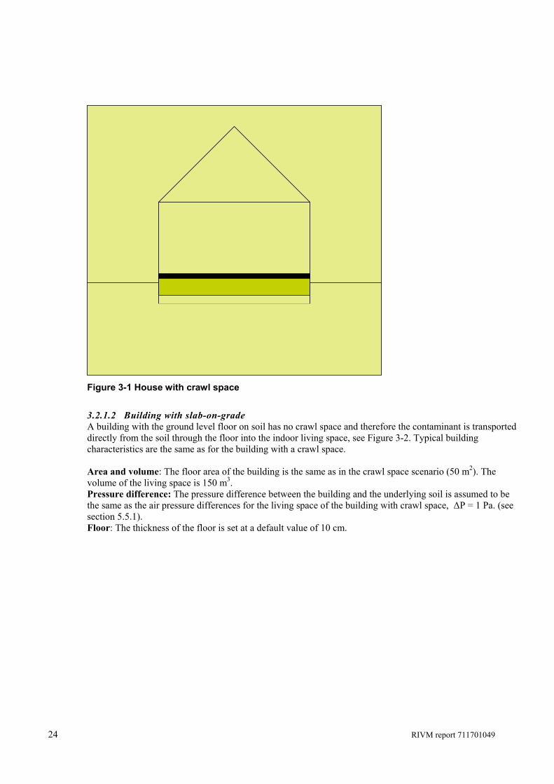
Figure 3-1 House with crawl space
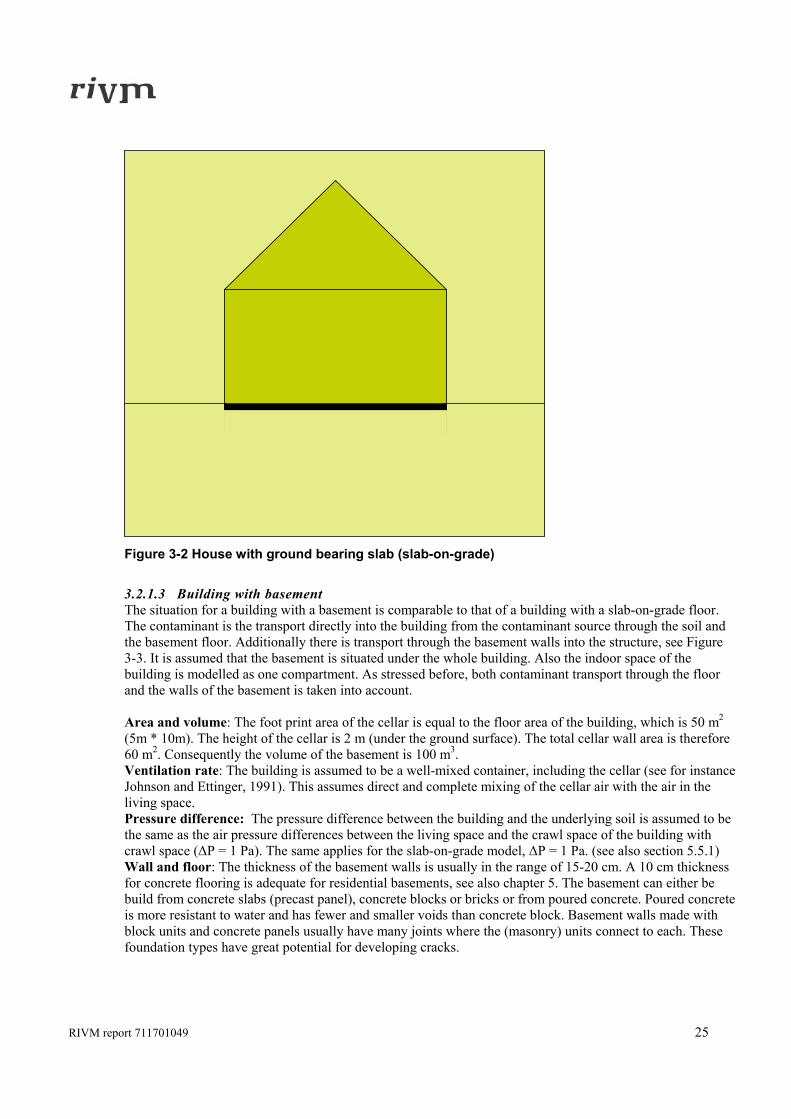
3.2.1.2 Building with slab-on-grade A building with the ground level floor on soil has no crawl space and therefore the contaminant is transported directly from the soil through the floor into the indoor living space, see Figure 3-2. Typical building characteristics are the same as for the building with a crawl space. Area and volume: The floor area of the building is the same as in the crawl space scenario (50 m2). The volume of the living space is 150 m3. Pressure difference: The pressure difference between the building and the underlying soil is assumed to be the same as the air pressure differences for the living space of the building with crawl space, ΔP = 1 Pa. (see section 5.5.1). Floor: The thickness of the floor is set at a default value of 10 cm.
RIVM report 711701049 25
Figure 3-2 House with ground bearing slab (slab-on-grade)
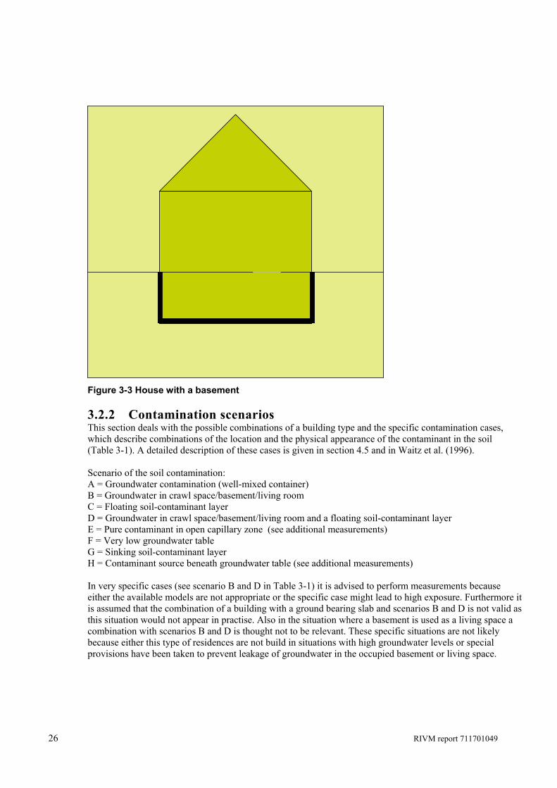
3.2.1.3 Building with basement The situation for a building with a basement is comparable to that of a building with a slab-on-grade floor. The contaminant is the transport directly into the building from the contaminant source through the soil and the basement floor. Additionally there is transport through the basement walls into the structure, see Figure 3-3. It is assumed that the basement is situated under the whole building. Also the indoor space of the building is modelled as one compartment. As stressed before, both contaminant transport through the floor and the walls of the basement is taken into account. Area and volume: The foot print area of the cellar is equal to the floor area of the building, which is 50 m2 (5m * 10m). The height of the cellar is 2 m (under the ground surface). The total cellar wall area is therefore 60 m2. Consequently the volume of the basement is 100 m3. Ventilation rate: The building is assumed to be a well-mixed container, including the cellar (see for instance Johnson and Ettinger, 1991). This assumes direct and complete mixing of the cellar air with the air in the living space. Pressure difference: The pressure difference between the building and the underlying soil is assumed to be the same as the air pressure differences between the living space and the crawl space of the building with crawl space (ΔP = 1 Pa). The same applies for the slab-on-grade model, ΔP = 1 Pa. (see also section 5.5.1) Wall and floor: The thickness of the basement walls is usually in the range of 15-20 cm. A 10 cm thickness for concrete flooring is adequate for residential basements, see also chapter 5. The basement can either be build from concrete slabs (precast panel), concrete blocks or bricks or from poured concrete. Poured concrete is more resistant to water and has fewer and smaller voids than concrete block. Basement walls made with block units and concrete panels usually have many joints where the (masonry) units connect to each. These foundation types have great potential for developing cracks.
26 RIVM report 711701049
Figure 3-3 House with a basement
3.2.2 Contamination scenarios This section deals with the possible combinations of a building type and the specific contamination cases, which describe combinations of the location and the physical appearance of the contaminant in the soil (Table 3-1). A detailed description of these cases is given in section 4.5 and in Waitz et al. (1996). Scenario of the soil contamination: A = Groundwater contamination (well-mixed container) B = Groundwater in crawl space/basement/living room C = Floating soil-contaminant layer D = Groundwater in crawl space/basement/living room and a floating soil-contaminant layer E = Pure contaminant in open capillary zone (see additional measurements) F = Very low groundwater table G = Sinking soil-contaminant layer H = Contaminant source beneath groundwater table (see additional measurements) In very specific cases (see scenario B and D in Table 3-1) it is advised to perform measurements because either the available models are not appropriate or the specific case might lead to high exposure. Furthermore it is assumed that the combination of a building with a ground bearing slab and scenarios B and D is not valid as this situation would not appear in practise. Also in the situation where a basement is used as a living space a combination with scenarios B and D is thought not to be relevant. These specific situations are not likely because either this type of residences are not build in situations with high groundwater levels or special provisions have been taken to prevent leakage of groundwater in the occupied basement or living space.
RIVM report 711701049 27
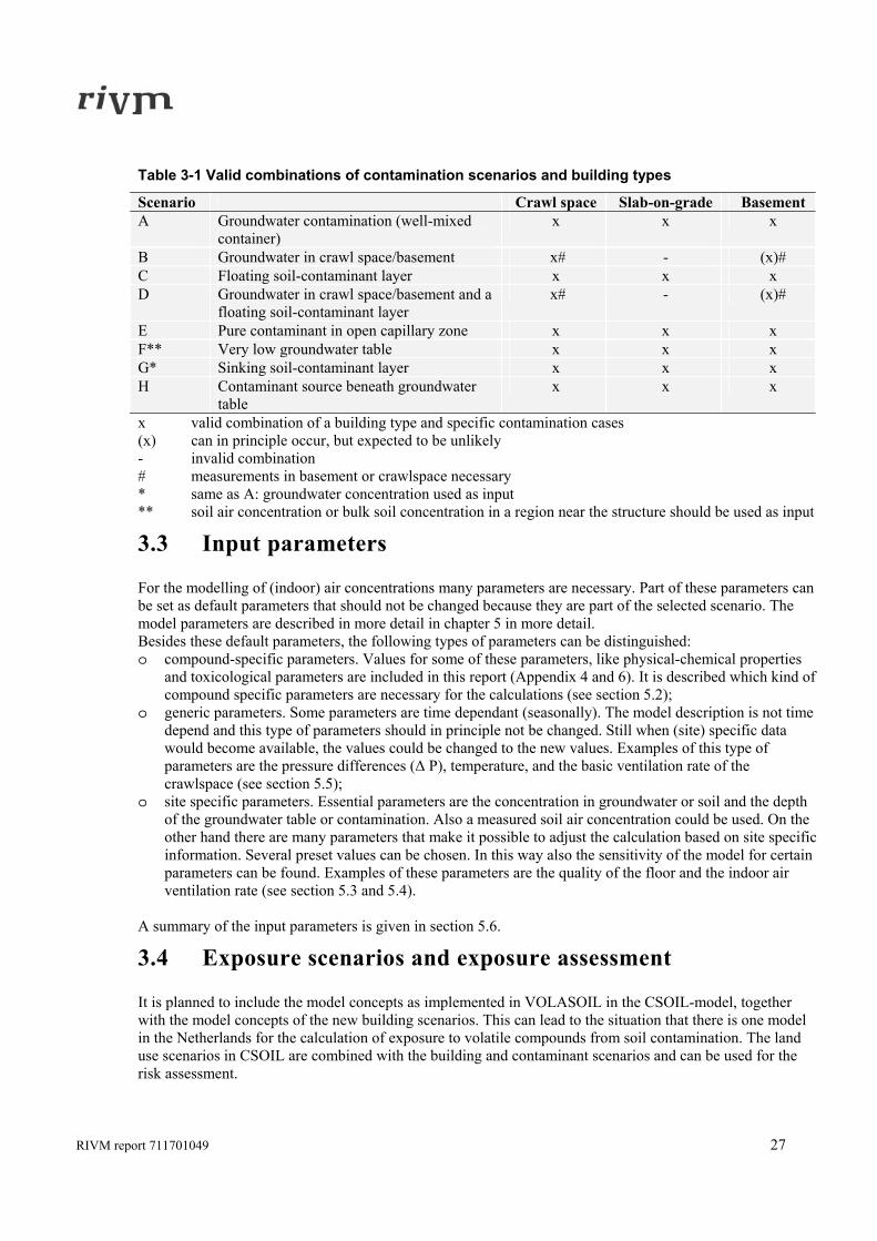
Table 3-1 Valid combinations of contamination scenarios and building types
Scenario Crawl space Slab-on-grade Basement A Groundwater contamination (well-mixed
container) x x x
B Groundwater in crawl space/basement x# - (x)# C Floating soil-contaminant layer x x x D Groundwater in crawl space/basement and a
floating soil-contaminant layer x# - (x)#
E Pure contaminant in open capillary zone x x x F** Very low groundwater table x x x G* Sinking soil-contaminant layer x x x H Contaminant source beneath groundwater
table x x x
x valid combination of a building type and specific contamination cases (x) can in principle occur, but expected to be unlikely - invalid combination # measurements in basement or crawlspace necessary * same as A: groundwater concentration used as input ** soil air concentration or bulk soil concentration in a region near the structure should be used as input
3.3 Input parameters For the modelling of (indoor) air concentrations many parameters are necessary. Part of these parameters can be set as default parameters that should not be changed because they are part of the selected scenario. The model parameters are described in more detail in chapter 5 in more detail. Besides these default parameters, the following types of parameters can be distinguished: o compound-specific parameters. Values for some of these parameters, like physical-chemical properties
and toxicological parameters are included in this report (Appendix 4 and 6). It is described which kind of compound specific parameters are necessary for the calculations (see section 5.2);
o generic parameters. Some parameters are time dependant (seasonally). The model description is not time depend and this type of parameters should in principle not be changed. Still when (site) specific data would become available, the values could be changed to the new values. Examples of this type of parameters are the pressure differences (Δ P), temperature, and the basic ventilation rate of the crawlspace (see section 5.5);
o site specific parameters. Essential parameters are the concentration in groundwater or soil and the depth of the groundwater table or contamination. Also a measured soil air concentration could be used. On the other hand there are many parameters that make it possible to adjust the calculation based on site specific information. Several preset values can be chosen. In this way also the sensitivity of the model for certain parameters can be found. Examples of these parameters are the quality of the floor and the indoor air ventilation rate (see section 5.3 and 5.4).
A summary of the input parameters is given in section 5.6.
3.4 Exposure scenarios and exposure assessment It is planned to include the model concepts as implemented in VOLASOIL in the CSOIL-model, together with the model concepts of the new building scenarios. This can lead to the situation that there is one model in the Netherlands for the calculation of exposure to volatile compounds from soil contamination. The land use scenarios in CSOIL are combined with the building and contaminant scenarios and can be used for the risk assessment.
28 RIVM report 711701049
It is recommended to differentiate between two exposure scenarios. The first is ‘residential’ land use, in which the exposure time is during the whole day (24 h). The TCA has not to be corrected. Secondly there is the land use with buildings in which people only stay during the working day (at the most 8 hours per day, 5 days a week). The calculated relevant air concentration is therefore corrected with a factor 40/168. Only for compounds for which the acute toxicity is equal to the chronic toxicity (e.g. cyanide, see Lijzen et al., in prep), this should not be done. When the assessment of volatile compounds is integrated in the exposure assessment of other exposure routes, the combined exposure to volatile compounds via indoor air and other exposure routes should be assessed. To take the other routes into account the sum of the exposure index to air and the exposure index to other exposure routes has a maximal value of 1.
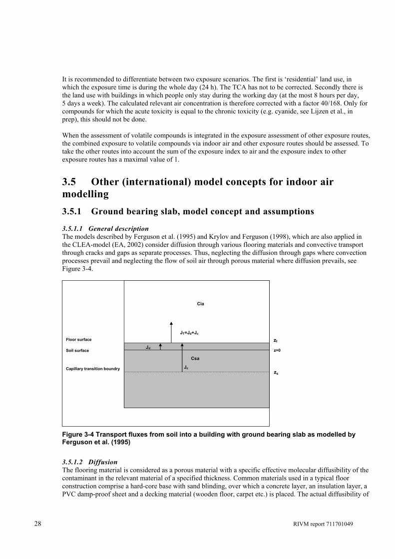
3.5 Other (international) model concepts for indoor air modelling 3.5.1 Ground bearing slab, model concept and assumptions 3.5.1.1 General description The models described by Ferguson et al. (1995) and Krylov and Ferguson (1998), which are also applied in the CLEA-model (EA, 2002) consider diffusion through various flooring materials and convective transport through cracks and gaps as separate processes. Thus, neglecting the diffusion through gaps where convection processes prevail and neglecting the flow of soil air through porous material where diffusion prevails, see Figure 3-4.
zf
z=0
zs Capillary transition boundry
Soil surface
Floor surface JT=Jd+Jc
Csa
Jc
Jd
Cia
Figure 3-4 Transport fluxes from soil into a building with ground bearing slab as modelled by Ferguson et al. (1995)
3.5.1.2 Diffusion The flooring material is considered as a porous material with a specific effective molecular diffusibility of the contaminant in the relevant material of a specified thickness. Common materials used in a typical floor construction comprise a hard-core base with sand blinding, over which a concrete layer, an insulation layer, a PVC damp-proof sheet and a decking material (wooden floor, carpet etc.) is placed. The actual diffusibility of
RIVM report 711701049 29
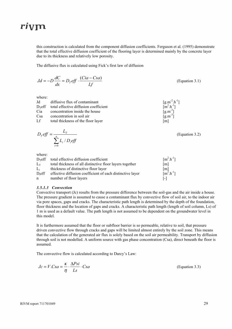
this construction is calculated from the component diffusion coefficients. Ferguson et al. (1995) demonstrate that the total effective diffusion coefficient of the flooring layer is determined mainly by the concrete layer due to its thickness and relatively low porosity. The diffusive flux is calculated using Fick’s first law of diffusion
LfCsaCiaeffD
dxdCDJd T
)( −⋅=−= (Equation 3.1)
where: Jd diffusive flux of contaminant [g.m-2.h-1] DTeff total effective diffusion coefficient [m2.h-1] Cia concentration inside the house [g.m-3] Csa concentration in soil air [g.m-3] Lf total thickness of the floor layer [m]
∑=
= n
iii
TT
effDL
LeffD
0/
(Equation 3.2)
where: DTeff total effective diffusion coefficient [m2.h-1] LT total thickness of all distinctive floor layers together [m] Li thickness of distinctive floor layer [m] Dieff effective diffusion coefficient of each distinctive layer [m2.h-1] n number of floor layers [-] 3.5.1.3 Convection Convective transport (Jc) results from the pressure difference between the soil-gas and the air inside a house. The pressure gradient is assumed to cause a contaminant flux by convective flow of soil air, to the indoor air via pore spaces, gaps and cracks. The characteristic path length is determined by the depth of the foundation, floor thickness and the location of gaps and cracks. A characteristic path length (length of soil column, Ls) of 1 m is used as a default value. The path length is not assumed to be dependent on the groundwater level in this model. It is furthermore assumed that the floor or subfloor barrier is so permeable, relative to soil, that pressure driven convective flow through cracks and gaps will be limited almost entirely by the soil zone. This means that the calculation of the generated air flux is solely based on the soil air permeability. Transport by diffusion through soil is not modelled. A uniform source with gas phase concentration (Csa), direct beneath the floor is assumed. The convective flow is calculated according to Darcy’s Law:
CsaLsPsiCsaVJc ⋅Δ⋅==
ηκ. (Equation 3.3)
30 RIVM report 711701049
where: Jc convective flux of the contaminant [g.m-2.h-1] V air flux from soil to indoor space [m3.m-2.h-1] Csa concentration in the soil-air [g.m-3] κ air permeability of soil [m2] η dynamic viscosity of air [Pa.h] ΔPsi air pressure difference between indoor air and soil [Pa] Ls characteristic path length for convection [m]
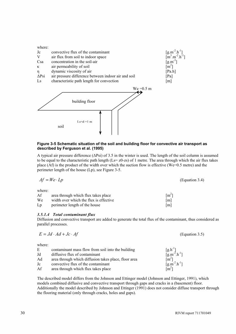
Figure 3-5 Schematic situation of the soil and building floor for convective air transport as described by Ferguson et al. (1995)
A typical air pressure difference (ΔPsi) of 3.5 in the winter is used. The length of the soil column is assumed to be equal to the characteristic path length (Ls= z0-zs) of 1 metre. The area through which the air flux takes place (Af) is the product of the width over which the suction flow is effective (We=0.5 metre) and the perimeter length of the house (Lp), see Figure 3-5. LpWeAf ⋅= (Equation 3.4) where: Af area through which flux takes place [m2] We width over which the flux is effective [m] Lp perimeter length of the house [m] 3.5.1.4 Total contaminant flux Diffusion and convective transport are added to generate the total flux of the contaminant, thus considered as parallel processes. AfJcAdJdE ⋅+⋅= (Equation 3.5) where: E contaminant mass flow from soil into the building [g.h-1] Jd diffusive flux of contaminant [g.m-2.h-1] Ad area through which diffusion takes place, floor area [m2] Jc convective flux of the contaminant [g.m-2.h-1] Af area through which flux takes place [m2] The described model differs from the Johnson and Ettinger model (Johnson and Ettinger, 1991), which models combined diffusive and convective transport through gaps and cracks in a (basement) floor. Additionally the model described by Johnson and Ettinger (1991) does not consider diffuse transport through the flooring material (only through cracks, holes and gaps).
We =0.5 m
building floor
soil Ls=d =1 m
RIVM report 711701049 31
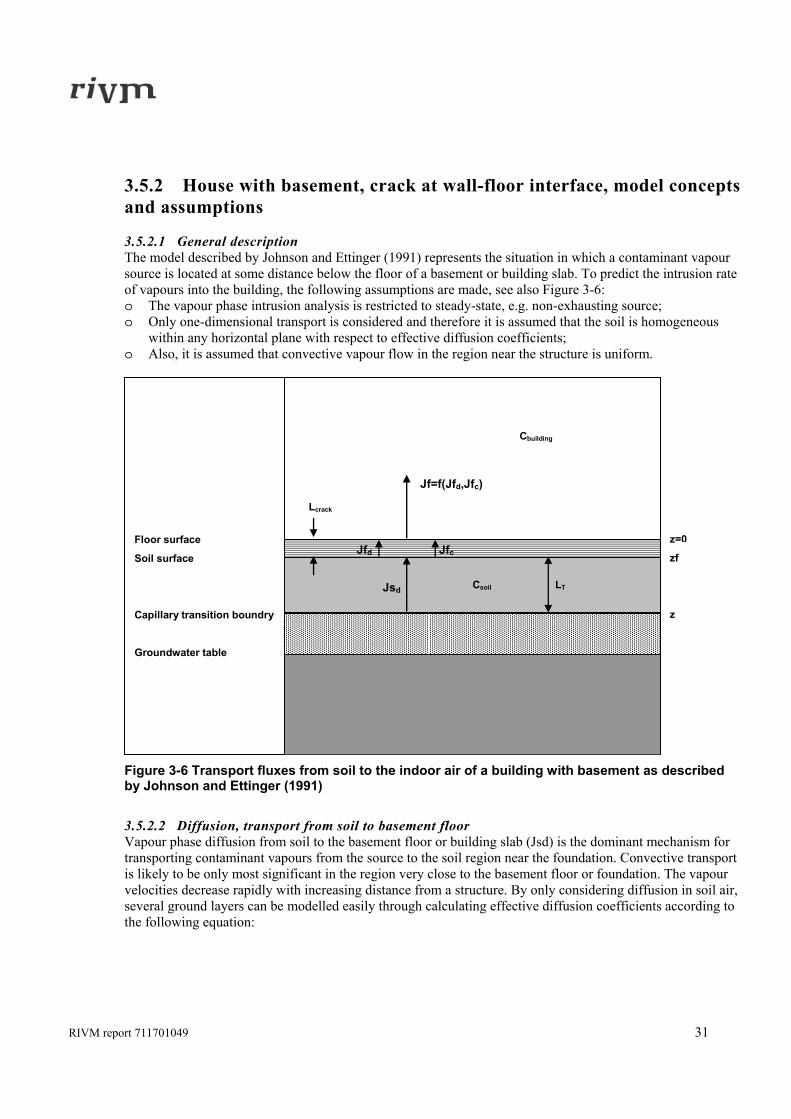
3.5.2 House with basement, crack at wall-floor interface, model concepts and assumptions 3.5.2.1 General description The model described by Johnson and Ettinger (1991) represents the situation in which a contaminant vapour source is located at some distance below the floor of a basement or building slab. To predict the intrusion rate of vapours into the building, the following assumptions are made, see also Figure 3-6: o The vapour phase intrusion analysis is restricted to steady-state, e.g. non-exhausting source; o Only one-dimensional transport is considered and therefore it is assumed that the soil is homogeneous
within any horizontal plane with respect to effective diffusion coefficients; o Also, it is assumed that convective vapour flow in the region near the structure is uniform.
Groundwater table
Capillary transition boundry
Soil surface
Floor surface
Jsd
Jf=f(Jfd,Jfc)
Jfc Jfd zf
z
z=0
LT
Lcrack
Csoil
Cbuilding
Figure 3-6 Transport fluxes from soil to the indoor air of a building with basement as described by Johnson and Ettinger (1991)
3.5.2.2 Diffusion, transport from soil to basement floor Vapour phase diffusion from soil to the basement floor or building slab (Jsd) is the dominant mechanism for transporting contaminant vapours from the source to the soil region near the foundation. Convective transport is likely to be only most significant in the region very close to the basement floor or foundation. The vapour velocities decrease rapidly with increasing distance from a structure. By only considering diffusion in soil air, several ground layers can be modelled easily through calculating effective diffusion coefficients according to the following equation:
32 RIVM report 711701049
∑=
= n
iii
TT
effDL
LeffD
0
(Equation 3.6)
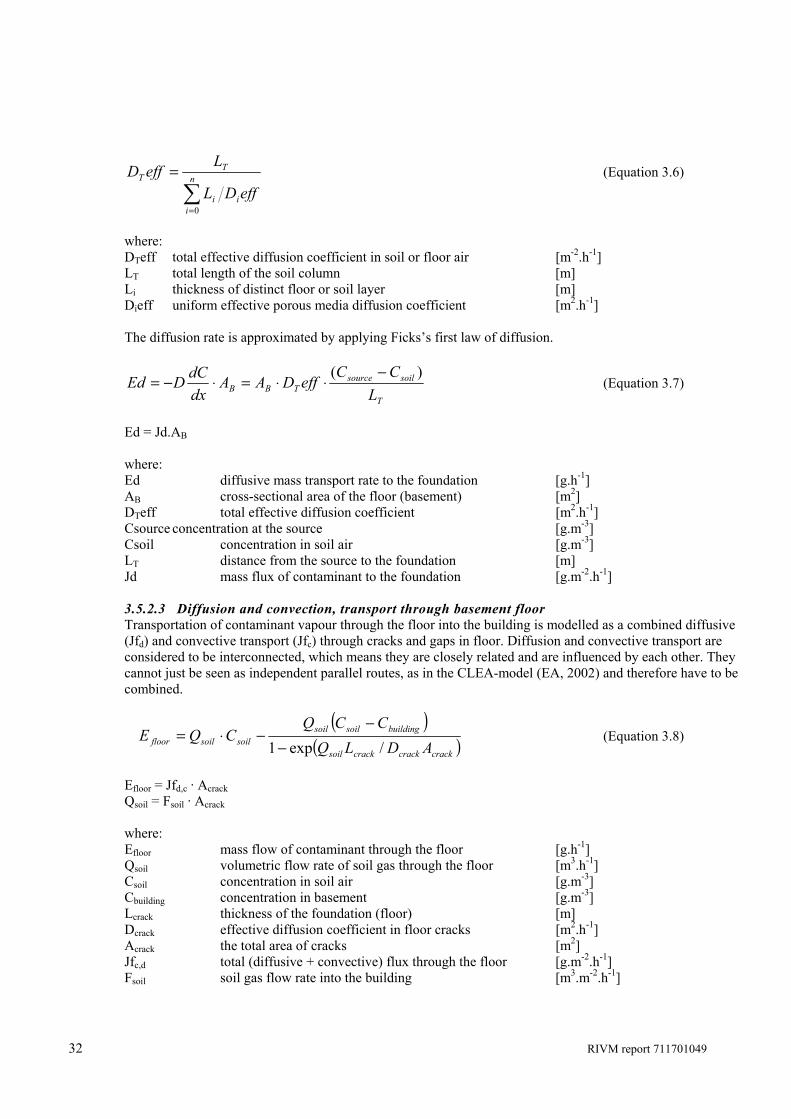
where: DTeff total effective diffusion coefficient in soil or floor air [m-2.h-1] LT total length of the soil column [m] Li thickness of distinct floor or soil layer [m] Dieff uniform effective porous media diffusion coefficient [m2.h-1] The diffusion rate is approximated by applying Ficks’s first law of diffusion.
T
soilsourceTBB L
CCeffDAA
dxdCDEd
)( −⋅⋅=⋅−= (Equation 3.7)
Ed = Jd.AB where: Ed diffusive mass transport rate to the foundation [g.h-1] AB cross-sectional area of the floor (basement) [m2] DTeff total effective diffusion coefficient [m2.h-1] Csource concentration at the source [g.m-3] Csoil concentration in soil air [g.m-3] LT distance from the source to the foundation [m] Jd mass flux of contaminant to the foundation [g.m-2.h-1] 3.5.2.3 Diffusion and convection, transport through basement floor Transportation of contaminant vapour through the floor into the building is modelled as a combined diffusive (Jfd) and convective transport (Jfc) through cracks and gaps in floor. Diffusion and convective transport are considered to be interconnected, which means they are closely related and are influenced by each other. They cannot just be seen as independent parallel routes, as in the CLEA-model (EA, 2002) and therefore have to be combined.
( )( )crackcrackcracksoil
buildingsoilsoilsoilsoilfloor ADLQ
CCQCQE
/exp1−−
−⋅= (Equation 3.8)
Efloor = Jfd,c · Acrack Qsoil = Fsoil · Acrack where: Efloor mass flow of contaminant through the floor [g.h-1] Qsoil volumetric flow rate of soil gas through the floor [m3.h-1] Csoil concentration in soil air [g.m-3] Cbuilding concentration in basement [g.m-3] Lcrack thickness of the foundation (floor) [m] Dcrack effective diffusion coefficient in floor cracks [m2.h-1] Acrack the total area of cracks [m2] Jfc,d total (diffusive + convective) flux through the floor [g.m-2.h-1] Fsoil soil gas flow rate into the building [m3.m-2.h-1]
RIVM report 711701049 33
The cracks and openings are assumed to be filled with dust and soil characterised by a density, porosity, and moisture content similar to that of the underlying soil. The effective diffusion coefficient Dcrack can therefore be estimated from these underlying soil parameters. 3.5.2.4 Perimeter gap model Contaminant vapours enter structures primarily through cracks and openings in the walls and foundation (electrical outlets, wall-floor seams, sump drains, et cetera). The soil gas flow rate is estimated by applying the solution derived by Nazaroff (1988) which actually applies to the situation of a peripheral gap between the basement floor and wall. Here the soil gas flow rate depends on soil properties, basement crack area, the basement geometry and building under pressure:
[ ] [ ]crackcrack
crackv
crackcrack
crackvsoil rZ
XPkrZ
XPkQ
/2ln2
/2ln2 π
μμπ
⋅Δ
=Δ
= (Equation 3.9)
where: Qsoil flow rate of soil vapour [m3.h] ΔP air pressure difference between soil and indoor air [Pa] kv soil permeability to vapour flow [m2] Xcrack length of the cavity [m] μ dynamic viscosity of air [Pa.h] Zcrack depth of the cavity below soil surface [m] rcrack equivalent radius of the cavity [m]
crack
Bcrack X
Ar η= (Equation 3.10)
where: rcrack radius of the cavity [m] η ratio between crack area and floor area Acrack/AB [-] AB enclosed area of the basement [m2] Xcrack length of the cavity [m] The crack ratio (η) and the crack width are related following:
Bcrack AW /4 ⋅=η (Equation 3.11) where: Wcrack width of the perimeter seam gap [m] AB enclosed area of the floor (basement) [m2] The major limitation to practical applications of the model is the lack of site specific values for η. It is not likely that such values can be easily measured (Johnson and Ettinger, 1991). 3.5.2.5 Porous material model, diffusion and convection Combined diffusive and convective transport through permeable (porous) material, rather than through foundation cracks and openings can also be modelled, see also Garbesi and Sextro (1989).
( )
( )Bfloorfloorsoil
buildingsoilsoilsoilsoilfloor ADLQ
CCQCQE
⋅−−
−⋅=/exp1
(Equation 3.12)
34 RIVM report 711701049
Efloor = Jfd,c.AB Qsoil = Fsoil.AB where: Efloor mass transport rate of contaminant into the building [g.h-1] Qsoil volumetric soil gas flow rate into the building [m3.h-1] Csoil concentration in soil air [g.m-3] Cbuilding concentration in basement [g.m-3] Lfloor thickness of the foundation (floor and walls) [m] Dfloor effective diffusion coefficient through porous floor [m-2.h-1] Jfd,c total contaminant flux into the building [g.m-2.h-1] AB total area of the basement floor and walls [m2] Fsoil soil gas flux into the building [m3.m-2.h-1] All contaminant vapours originating from directly below the basement will enter the basement, unless the floor and walls are perfect vapour barriers. Garbesi and Sextro (1989) stress that even in houses that do have a wall-floor gap in the basement, transport through porous below-grade walls might dominate soil-gas entry. Their research suggests that, in sufficient permeable soils, under normal house operating conditions, subsurface entry of soil gas into houses could be significant elevated by transport through permeable walls. 3.5.2.6 Discussion The equations for combined diffusive and convective transport through cracks and openings or through porous material appear similar though can predict quite different results. The equation for combined diffusive and convective transport through porous material is independent of the area of cracks/openings because intrusion is assumed to occur uniformly over the floor/wall area. For a given Fsoil therefore, the soil gas velocity through the floor/walls is lower for the permeable floor/wall case. The impact of this is that the equation for porous material may predict that transport through the foundation is diffusion dominated, while the equation for cracks/openings predicts that it is convective dominated, for a given Fsoil and diffusion coefficient. The model described by Johnson and Ettinger (1991) considers also the basement walls to be contributing to the contaminant transport into the building. The air flow rate into the building is considered to be corresponding to a volume exchange rate of 0.5 per hour.
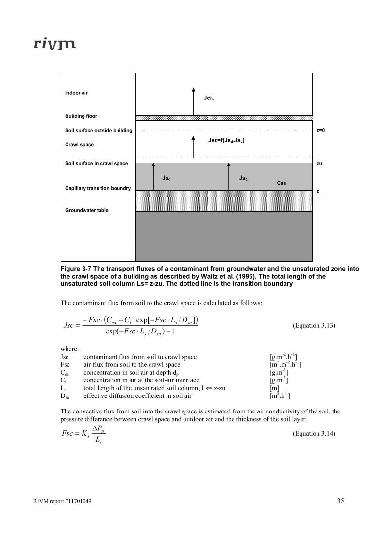
3.5.3 House with crawl space The VOLASOIL-model (Waitz et al 1996) describes the transport of a soil contaminant from below a building with crawl space into that building. The contaminant is transported from the unsaturated groundwater zone to the crawl space and from the crawl space through the building floor into the indoor living space. The model concept reflects a steady-state situation with one dimensional transport from a non-exhausting source. Degradation of the contaminant is not considered. Transport through the unsaturated zone (from soil into crawl space) is modelled as a combined interrelated diffusive and convective transport through the soil air phase (see also Figure 3-7). The contaminant with concentration Csa in the soil air of the open capillary zone (unsaturated zone) is located at depth z. At the upper boundary of the unsaturated zone (transition from the soil column to the crawl space air) the depth is zu, the concentration is equal to Ci. The soil surface outside the building is at z=0.
RIVM report 711701049 35
Groundwater zone
Full capillary zone
Open capillary zone
Boundary layer
Housing floor
Groundwater table
Capillary transition boundry
Soil surface in crawl space
Jsd
Jsc=f(Jsd,Jsc)
Jsc
zu
z
z=0
Jcic
Crawl space
Indoor air
Building floor
Soil surface outside building
Csa
Figure 3-7 The transport fluxes of a contaminant from groundwater and the unsaturated zone into the crawl space of a building as described by Waitz et al. (1996). The total length of the unsaturated soil column Ls= z-zu. The dotted line is the transition boundary
The contaminant flux from soil to the crawl space is calculated as follows:
( )
1)exp(]exp[
−⋅−⋅−⋅−⋅−
=sas
sasisa
DLFscDLFscCCFsc
Jsc (Equation 3.13)
where: Jsc contaminant flux from soil to crawl space [g.m-2.h-1] Fsc air flux from soil to the crawl space [m3.m-2.h-1] Csa concentration in soil air at depth dp [g.m-3] Ci concentration in air at the soil-air interface [g.m-3] Ls total length of the unsaturated soil column, Ls= z-zu [m] Dsa effective diffusion coefficient in soil air [m2.h-1] The convective flux from soil into the crawl space is estimated from the air conductivity of the soil, the pressure difference between crawl space and outdoor air and the thickness of the soil layer.
s
css L
PKFsc
Δ= (Equation 3.14)
36 RIVM report 711701049
where: Fsc air flux from soil into crawl space [m3.m-2.h-1] Ks air conductivity of the soil layer [m2.Pa-1.h-1] ΔPcs pressure difference between crawl space and soil [Pa] Ls thickness of the soil layer [m] Diffusion through the soil layer is estimated from the diffusion coefficient in free air.
( )23/10
1 s
aasa V
DVD
−= (Equation 3.15)
where: Dsa diffusion coefficient in soil air [m2.h-1] Va volume fraction soil air [-] Da diffusion coefficient in free air [m2.h-1] Vs volume fraction of solids [-] The convective flow through the floor (from crawl space to indoor air) is modelled as convective transport through gaps and holes in the floor by combining Poiseuille’s law for laminar flow through cylindrical tubes and Darcy’s law. Diffusion through the floor (porous media or diffusion through gaps, cracks and holes) is not considered.
f
icof
f
icf L
Pn
fLP
KFciΔ
⋅=
Δ=
ηπ 8
2
(Equation 3.16)
where: Fci air flux from crawl space to the indoor space [m3.m-2.h-1] Kf air conductivity of floor [m2.Pa-1.h-1] ΔPic pressure difference between indoor space and crawl space [Pa] Lf thickness of the floor [m] fof fraction of openings in floor [m2.m-2] n number of opening per floor area [m-2] η dynamic viscosity of air [Pa.h] Waitz et al. (1996) give values for fof for various floor qualities, see Table 5-15. The contaminant flux is calculated from the concentration in the crawl space and the air flux.
caCFciJci ⋅= (Equation 3.17) where: Jci contaminant flux from crawl space to the indoor space [g.m-2.h-1] Fci air flux from crawl space to the indoor space [m3.m-2.h-1] Cca concentration in crawl space air [g.m-3]
RIVM report 711701049 37
The approaches for modelling contaminant transport through soil and through the housing floor without the intermediate crawl space, can be combined to model the situation of building with a ground-bearing slab. This approach leads to a model with interrelated convective and diffusive transport through the unsaturated zone and only convective transport through the housing floor as describe by Waitz et al. (1996) without the intervening crawl space. This will be elaborated in chapter 4, where a new model for buildings with a slab-on-grade floor will be described.
3.5.4 General discussion on model concepts Basically the models apply different approaches in modelling vapour transport through soil and through the ground floor of the building. Either diffusion or convection are considered as separate or combined processes depending on the anticipated situation to be modelled or pre-assumptions on the expected dominance of one or the other transport mechanism. Specifically for floor transport, it is either thought to take place through pores or artificial openings in the foundation slab. One of the models describes transport through both pores and openings, but considers only diffusion to be relevant for transport through the pores and convection only being relevant for gaps and cracks For modelling transport through the floor three concepts can be distinguished from the models that have been studied. The porous medium concept, the gap model and the perimeter seam gap model: The porous medium concept uses the effective diffusion coefficient to determine actual diffusion for multiple layers. Convective transport through porous media can be described by applying de measured air permeability coefficient for the specific material (Darcy’s law); The gap model uses a combination of Poiseuilles law for the laminar flow through a cylinder and Darcy’s law to calculate convective flow through gaps in a floor; Thirdly the ‘perimeter seam gap’ model describes the specific situation for convective transport through a perimeter seam gap. This concept may be applicable for both basements and slab-on-grade floors. All three concepts may be applicable for the three building types, slab-on-grade, crawl space and basement. Their specific applicability depends on the actual situation and which model is the most representative. Intact floors from newly build residences with no pipe ducts or crawl space hatch and free from shrinkage cracks can be modelled by applying the porous medium concepts. The gap model is most representative for residence with a crawl space and/ or having pipe ducts through the floor. The perimeter seam gap model can be applied in the situation of residences with a basement or ground bearing slab having seam gaps either only along the perimeter or linear cracks in the horizontal plain (either longitudinal or cross-sectional). Optionally the contribution of permeable basement walls to the total soil gas entry can be added to the contribution calculated by perimeter seam gap model following the suggestion of Garbesi and Sextro (1989). Therefore, this is added to the model as an extra option to include in the calculations.

38 RIVM report 711701049
RIVM report 711701049 39
4. Model concepts for different types of buildings
4.1 Introduction In chapter 3, from existing model descriptions, three different basic concepts or model representations for modelling the transport of volatile contaminants from soil into buildings have been deduced. These representations refer to some extend to the way buildings are build, but basically relate to the occurrence of prevalent transport routes, being cracks (along the perimeter of the floor), holes or pores, which are present in the building floor. Depending on the actual situation either of the approaches applies. Furthermore volatile compounds can be transported through diffusion or convective flow. For each concept both diffusion and convective flow are taken into account. Which process is dominant actually depends on the soil properties, the properties of the building elements and the characteristics of the cracks, holes that are present. The model concepts are discussed in this chapter in combination with the three different building types e.g. residence with a crawl space, slab-on-grade floor and a basement. In section 4.5 the contamination scenarios are explained and is is described how sources depletion can be judged.
4.2 Building with crawlspace The VOLASOIL model has already briefly being described in chapter 3; in this section the model is described in more detail. The formulation of the original model is maintained and the formulation of the new model concepts will be in accordance with it as much as possible.
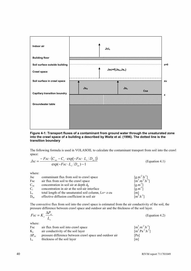
4.2.1 Transport from soil/groundwater to the crawlspace The VOLASOIL-model describes the transport of a contaminant in soil or groundwater from a location below a building into that building. The contaminant is transported from the unsaturated groundwater zone to the crawl space and from the crawl space through the building floor into the indoor living space. The model concept reflects a steady-state situation with one dimensional transport from a non-exhausting source. Degradation of the contaminant is not considered. Transport through the unsaturated zone is modelled as a combined and interrelated diffusive and convective transport through the soil air phase (see also Figure 4-1). The contaminant with concentration Csa in the soil air of the open capillary zone (unsaturated zone) is located at depth z. At the upper boundary of the unsaturated zone (transition from the soil column to the crawl space air), at z=zu, the concentration is equal to Ci. The soil surface outside the building is at z=0.
40 RIVM report 711701049
Groundwater zone
Full capillary zone
Open capillary zone
Boundary layer
Housing floor
Groundwater table
Capillary transition boundry
Soil surface in crawl space
Jsd
Jsc=f(Jsd,Jsc)
Jsc
zu
z
z=0
Jcic
Crawl space
Indoor air
Building floor
Soil surface outside building
Csa
Figure 4-1: Transport fluxes of a contaminant from ground water through the unsaturated zone into the crawl space of a building a described by Waitz et al. (1996). The dotted line is the transition boundary
The following formula is used in VOLASOIL to calculate the contaminant transport from soil into the crawl space:
( )1)exp(
]exp[−⋅−⋅−⋅−⋅−
=sas
sasisa
DLFscDLFscCCFsc
Jsc (Equation 4.1)
where: Jsc contaminant flux from soil to crawl space [g.m-2.h-1] Fsc air flux from soil to the crawl space [m3.m-2.h-1] Csa concentration in soil air at depth dp [g.m-3] Ci concentration in air at the soil-air interface [g.m-3] Ls total length of the unsaturated soil column, Ls= z-zu [m] Dsa effective diffusion coefficient in soil air [m2.h-1] The convective flux from soil into the crawl space is estimated from the air conductivity of the soil, the pressure difference between crawl space and outdoor air and the thickness of the soil layer.
s
scs L
PKFsc
Δ= (Equation 4.2)
where: Fsc air flux from soil into crawl space [m3.m-2.h-1] Ks air conductivity of the soil layer [m2.Pa-1.h-1] ΔPcs pressure difference between crawl space and outdoor air [Pa] Ls thickness of the soil layer [m]
RIVM report 711701049 41
The length of the unsaturated soil column for a building with a crawl space equals the depth of the groundwater table (dg) minus the height of the capillary transition boundary (hcb) minus the depth of the crawl space beneath the soil surface (dc):
ccbgws dhdL −−= (Equation 4.3) where: Ls length of the unsaturated soil column [m] dgw depth of the groundwater table [m] hcb height of the capillary transition boundary [m] dc depth of the crawl space beneath soil surface [m] The length of the soil column should be at least several centimetres to prevent that the model calculates unrealistic high flow rates into the crawlspace. To calculate the contaminant transport from the crawl space into the building only convective transport across the building floor is considered in the VOLASOIL model. The convective flow through the floor is modelled as a flow of air through gaps and holes in the floor. Gaps and holes are modelled as tubes of uniform radius. Calculation of the air flux is done by combining Poiseulle’s law for laminar flow through cylindrical tubes and Darcy’s law, which yields the air conductivity of the floor (Kf). Diffusion through the floor (through the porous of the media or diffusion through gaps, cracks and holes) is not considered.
f
icof
f
icf L
Pn
fLP
KFciΔ
⋅=
Δ=
ηπ 8
2
(Equation 4.4)
where: Fci air flux from crawl space to the indoor space [m3.m-2.h-1] Kf air conductivity of floor [m2.Pa-1.h-1] ΔPic pressure difference between indoor space and crawl space [Pa] Lf thickness of the floor [m] fof fraction of openings in floor [m2.m-2] n number of opening per floor area [m-2] η dynamic viscosity of air [Pa.h] The contaminant flux from the crawl space through the floor into the indoor space is calculated as next:
caCFciJci ⋅= (Equation 4.5) where: Jci air flux from crawl space to the indoor space [g.m-2.h-1] Fci air flux from crawl space to indoor air [m3.m-2] Cca concentration in crawl space air [g.m-3]
42 RIVM report 711701049
4.2.2 Calculation of indoor air concentration, scenario crawlspace The concentration in the crawl space can be calculated on the basis of the total contaminant flux from the soil into the crawl space, the basic air-exchange rate of the crawl space and dimensions of the crawl space:
c
fbC,C V
AFscvvvv
⋅+= (Equation 4.6)
where: vvc air-exchange rate for crawl space [h-1] vvc,b basic air exchange rate for crawl space [h-1] Fsc air flux from soil into the crawl space [m3.m-2.h-1] Af surface area of the floor [m2] Vc volume of the crawl space [m3] The crawl space concentration is finally calculated from the contaminant flux into the indoor space and the basic air-exchange rate for the indoor space:
ic
fca vvV
AJscC
⋅⋅
= (Equation 4.7)
where: Cca crawl space air concentration [g.m-3] Jsc contaminant flux from soil into the crawl space [g.m-2.h-1] Af surface area of the floor [m2] Vc volume of the crawl space [m3] vvi air-exchange rate for indoor space [h-1] For calculating the indoor-air concentration for a building with a crawl space, the ventilation is expressed as an average air-exchange rate. The air-exchange rate can be calculated from the required ventilation properties for houses. The air-exchange rate is composed of the basic ventilation rate and the air flux through the building floor:
i
fbi,i V
AFcivvvv
⋅+= (Equation 4.8)
where: vvi air-exchange rate for indoor space [h-1] vvi,b basic air-exchange rate of indoor space [h-1] Fci air flux through the floor into the indoor space [m3.m-2.h-1] Af surface area of the floor [m2] Vi volume of the indoor space [m3] The indoor concentration is finally calculated from the contaminant flux into the indoor space and the basic air-exchange rate for the indoor space:
ii
fia vvV
AJciC
⋅⋅
= (Equation 4.9)
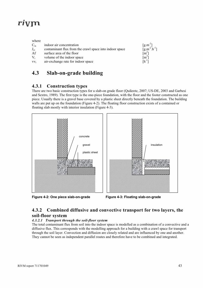
RIVM report 711701049 43
where Cia indoor air concentration [g.m-3] Jci contaminant flux from the crawl space into indoor space [g.m-2.h-1] Af surface area of the floor [m2] Vi volume of the indoor space [m3] vvi air-exchange rate for indoor space [h-1]
4.3 Slab-on-grade building
4.3.1 Construction types There are two basic construction types for a slab-on grade floor (Quikrete, 2007; US-DE, 2003 and Garbesi and Sextro, 1989). The first type is the one-piece foundation, with the floor and the footer constructed as one piece. Usually there is a gravel base covered by a plastic sheet directly beneath the foundation. The building walls are put up on the foundation (Figure 4-2). The floating floor construction exists of a contained or floating slab mostly with interior insulation (Figure 4-3).
Figure 4-2: One piece slab-on-grade Figure 4-3: Floating slab-on-grade
4.3.2 Combined diffusive and convective transport for two layers, the soil-floor system 4.3.2.1 Transport through the soil-floor system The total contaminant flux from soil into the indoor space is modelled as a combination of a convective and a diffusive flux. This corresponds with the modelling approach for a building with a crawl space for transport through the soil layer. Convection and diffusion are closely related and are influenced by one and another. They cannot be seen as independent parallel routes and therefore have to be combined and integrated.
gravel
concrete
plastic sheet
insulation
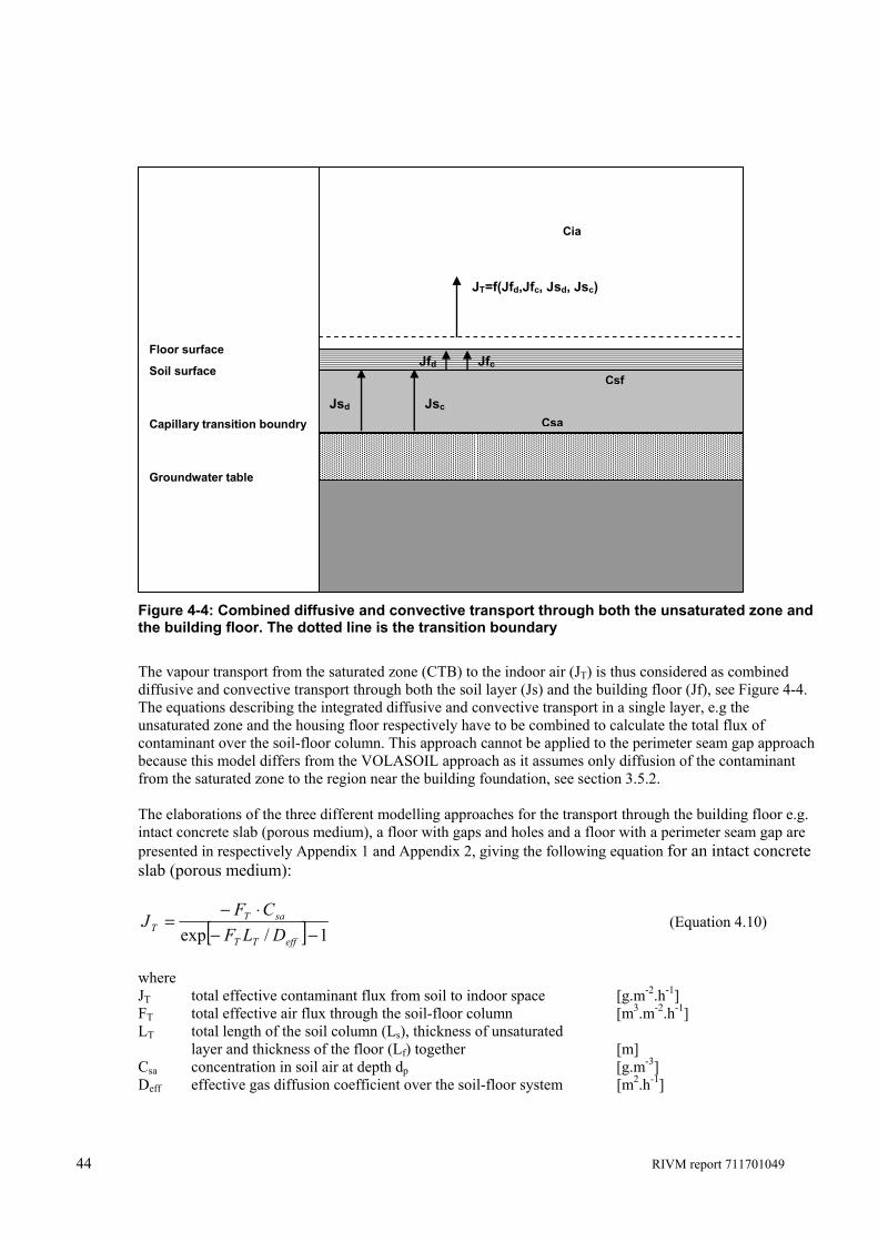
44 RIVM report 711701049
Groundwater table
Capillary transition boundry
Soil surface
Floor surface
Jsd
JT=f(Jfd,Jfc, Jsd, Jsc)
Jsc
Jfc Jfd
Csa
Csf
Cia
Figure 4-4: Combined diffusive and convective transport through both the unsaturated zone and the building floor. The dotted line is the transition boundary
The vapour transport from the saturated zone (CTB) to the indoor air (JT) is thus considered as combined diffusive and convective transport through both the soil layer (Js) and the building floor (Jf), see Figure 4-4. The equations describing the integrated diffusive and convective transport in a single layer, e.g the unsaturated zone and the housing floor respectively have to be combined to calculate the total flux of contaminant over the soil-floor column. This approach cannot be applied to the perimeter seam gap approach because this model differs from the VOLASOIL approach as it assumes only diffusion of the contaminant from the saturated zone to the region near the building foundation, see section 3.5.2. The elaborations of the three different modelling approaches for the transport through the building floor e.g. intact concrete slab (porous medium), a floor with gaps and holes and a floor with a perimeter seam gap are presented in respectively Appendix 1 and Appendix 2, giving the following equation for an intact concrete slab (porous medium):
[ ] 1/exp −−⋅−
=effTT
saTT DLF
CFJ (Equation 4.10)
where JT total effective contaminant flux from soil to indoor space [g.m-2.h-1] FT total effective air flux through the soil-floor column [m3.m-2.h-1] LT total length of the soil column (Ls), thickness of unsaturated
layer and thickness of the floor (Lf) together [m] Csa concentration in soil air at depth dp [g.m-3] Deff effective gas diffusion coefficient over the soil-floor system [m2.h-1]
RIVM report 711701049 45
For the situation of gaps and holes in the building floor, the VOLASOIL approach, the following equation can be derived:
[ ] [ ] 1/DLFexp/DLFexpCF
Jsassgapfgap
saff −⋅−⋅⋅−
⋅−= (Equation 4.11)
where: Jf contaminant flux through gaps in the slab (footprint area) [g.m-2.h-1] Ff air flux through the floor (foot print floor area) [m3.m-2.h-1] Csa concentration in soil air at depth dp [g.m-3] Fgap air flux through the holes and gaps (area of gaps) [m3.m-2.h-1] Dgap effective gas diffusion coefficient in gaps and holes [m2.h-1] Lf thickness of the floor [m] Fs air flux through the soil layer (foorprint area floor) [m3.m-2.h-1] Ls length of the soil column (thickness of unsaturated layer) [m] Dsa effective gas diffusion coefficient in soil air [m2.h-1] Finally, for the perimeter seam gap approach the following equation has been derived:
sasscrackfcrack
saff DLFDLF
CFJ
⋅−−−⋅−
=1)/exp(
(Equation 4.12)
where: Jf contaminant flux through perimeter seam gap (footprint area) [g.m-2.h-1] Ff air flux through the floor (foot print floor area) [m3.m-2.h-1] Csa concentration in soil air at depth dp [g.m-3] Fcrack air flux through the perimeter seam gap (per area of cracks) [m3.m-2.h-1] Dcrack gas diffusion coefficient in perimeter seam crack [m2.h-1] Lf thickness of the floor [m] Ls length of the soil column (thickness of unsaturated layer) [m] Fs air flux through the soil near the structure (area floor) [m3.m-2.h-1] Dsa effective gas diffusion coefficient in soil air [m2.h-1] As will be shown in section 4.3.4.3 the depth of the groundwater table is not used in the calculation of the air flow from the soil through the floor into the building in case of a perimeter seam gap. This is due to a difference in the modelling concept which is elaborated by Nazaroff (1988) and Johnson and Ettinger (1991). As indicated in section 3.5.2.2 for this model concept, transport from the source through the soil to the building foundation is assumed to be caused by diffusion only. The dominant convection route is assumed to be from the soil surface to the region near the building foundation. To the contrary, the VOLASOIL model concept assumes a convection route from the top of the capillary transition boundary to the building floor. Example calculations of each calculation method for the slab-on-grade building type are presented in Appendix 7. 4.3.2.2 Transport through saturated zone and the soil-floor column When there is a distinct contaminant source beneath the groundwater table (scenario H in section 3.2.2), transport fluxes in the open capillary zone will be limited by the contaminant supplying flux through the saturated zone. The contaminant first has to be transported through the saturated zone. It is assumed that this is only achieved by diffusive transport through the capillary zone and there is no water evaporation flux.
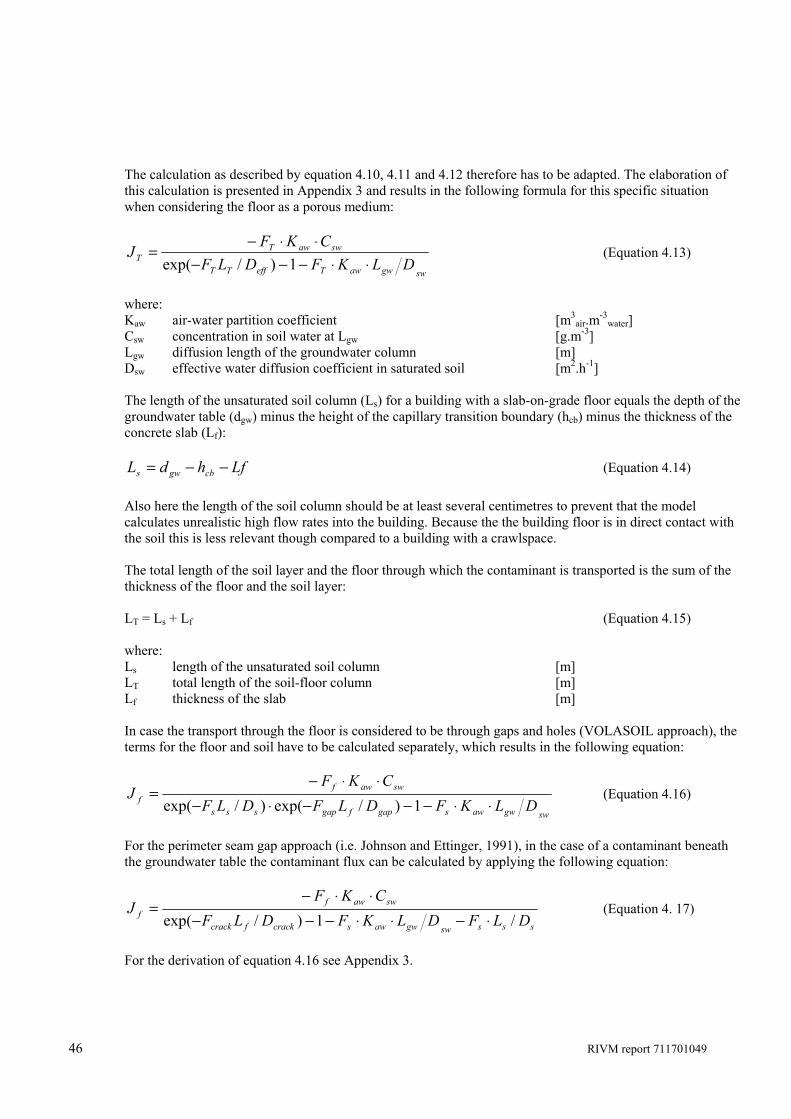
46 RIVM report 711701049
The calculation as described by equation 4.10, 4.11 and 4.12 therefore has to be adapted. The elaboration of this calculation is presented in Appendix 3 and results in the following formula for this specific situation when considering the floor as a porous medium:
swgwawTeffTT
swawTT DLKFDLF
CKFJ
⋅⋅−−−⋅⋅−
=1)/exp(
(Equation 4.13)
where: Kaw air-water partition coefficient [m3
air.m-3water]
Csw concentration in soil water at Lgw [g.m-3] Lgw diffusion length of the groundwater column [m] Dsw effective water diffusion coefficient in saturated soil [m2.h-1] The length of the unsaturated soil column (Ls) for a building with a slab-on-grade floor equals the depth of the groundwater table (dgw) minus the height of the capillary transition boundary (hcb) minus the thickness of the concrete slab (Lf):
LfhdL cbgws −−= (Equation 4.14) Also here the length of the soil column should be at least several centimetres to prevent that the model calculates unrealistic high flow rates into the building. Because the the building floor is in direct contact with the soil this is less relevant though compared to a building with a crawlspace. The total length of the soil layer and the floor through which the contaminant is transported is the sum of the thickness of the floor and the soil layer: LT = Ls + Lf (Equation 4.15) where: Ls length of the unsaturated soil column [m] LT total length of the soil-floor column [m] Lf thickness of the slab [m] In case the transport through the floor is considered to be through gaps and holes (VOLASOIL approach), the terms for the floor and soil have to be calculated separately, which results in the following equation:
swgwawsgapfgapsss
swawff DLKFDLFDLF
CKFJ
⋅⋅−−−⋅−⋅⋅−
=1)/exp()/exp(
(Equation 4.16)
For the perimeter seam gap approach (i.e. Johnson and Ettinger, 1991), in the case of a contaminant beneath the groundwater table the contaminant flux can be calculated by applying the following equation:
sssswgwawscrackfcrack
swawff DLFDLKFDLF
CKFJ
/1)/exp( ⋅−⋅⋅−−−⋅⋅−
= (Equation 4. 17)
For the derivation of equation 4.16 see Appendix 3.
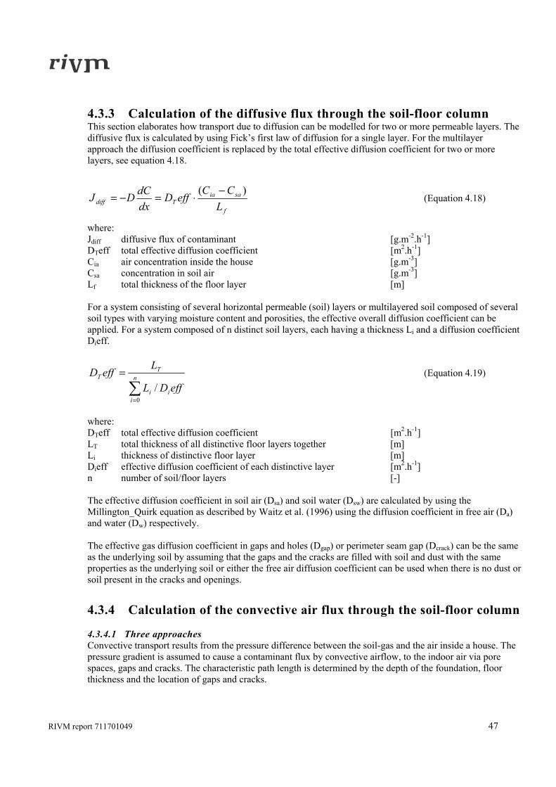
RIVM report 711701049 47
4.3.3 Calculation of the diffusive flux through the soil-floor column This section elaborates how transport due to diffusion can be modelled for two or more permeable layers. The diffusive flux is calculated by using Fick’s first law of diffusion for a single layer. For the multilayer approach the diffusion coefficient is replaced by the total effective diffusion coefficient for two or more layers, see equation 4.18.
f
saiaTdiff L
CCeffD
dxdCDJ
)( −⋅=−= (Equation 4.18)
where: Jdiff diffusive flux of contaminant [g.m-2.h-1] DTeff total effective diffusion coefficient [m2.h-1] Cia air concentration inside the house [g.m-3] Csa concentration in soil air [g.m-3] Lf total thickness of the floor layer [m] For a system consisting of several horizontal permeable (soil) layers or multilayered soil composed of several soil types with varying moisture content and porosities, the effective overall diffusion coefficient can be applied. For a system composed of n distinct soil layers, each having a thickness Li and a diffusion coefficient Dieff.
∑=
= n
iii
TT
effDL
LeffD
0/
(Equation 4.19)
where: DTeff total effective diffusion coefficient [m2.h-1] LT total thickness of all distinctive floor layers together [m] Li thickness of distinctive floor layer [m] Dieff effective diffusion coefficient of each distinctive layer [m2.h-1] n number of soil/floor layers [-] The effective diffusion coefficient in soil air (Dsa) and soil water (Dsw) are calculated by using the Millington_Quirk equation as described by Waitz et al. (1996) using the diffusion coefficient in free air (Da) and water (Dw) respectively. The effective gas diffusion coefficient in gaps and holes (Dgap) or perimeter seam gap (Dcrack) can be the same as the underlying soil by assuming that the gaps and the cracks are filled with soil and dust with the same properties as the underlying soil or either the free air diffusion coefficient can be used when there is no dust or soil present in the cracks and openings.
4.3.4 Calculation of the convective air flux through the soil-floor column 4.3.4.1 Three approaches Convective transport results from the pressure difference between the soil-gas and the air inside a house. The pressure gradient is assumed to cause a contaminant flux by convective airflow, to the indoor air via pore spaces, gaps and cracks. The characteristic path length is determined by the depth of the foundation, floor thickness and the location of gaps and cracks.

48 RIVM report 711701049
There are basically three ways of calculating the air flux through the floor:
the ‘capillary’ approach according to the VOLASOIL model (Waitz et al., 1996)); the ‘perimeter seam gap’model by Johnsonand Ettinger (1991) and the ‘orous media’ approach used by Krylov and Ferguson (1998).
The three approaches will be available in the adapted VOLASOIL model as a basis for comparison of the calculated results. It should be emphasised that the three modelling approaches represent three different cases, which might be difficult to compare, i.e., parameterisation is needed to represent the same actual case and might be difficult to achieve. 4.3.4.2 Air flux through intact floor (porous medium) The convective flow for a single (soil or floor) layer is calculated according to Darcy’s Law:
sas
sisaconv C
LP
CFsiJ ⋅Δ
⋅=⋅=ηκ
(Equation 4.20)
where: Jconv convective flux of the contaminant [g.m-2.h-1] Fsi air flux from soil to indoor space [m3.m-2.h-1] ΔPsi air pressure difference between indoor air and soil [Pa] Ls characteristic path length for convection [m] κ air permeability of soil [m2] η dynamic viscosity of air [Pa.h] Csa concentration in the soil-air [g.m-3] The air conductivity is calculated from the air permeability coefficients of the various layers (soil and concrete) according to following formula:
ηκ fs
fsK // = (Equation 4.21)
where: Ks/f air conductivity of material (soil or floor) [m2.Pa-1.h-1] κs/f air permeability of material (soil or floor) [m2] η dynamic viscosity of air [m2] The total convective flux FT is calculated according to equation 4.22, this formula gives the overall flux for two layers, the soil-floor system:
f
f
s
s
TT
KL
KL
PF+
Δ= (Equation 4.22)
where: FT overall air flux from the soil-floor column [m3.m-2.s-1] ΔPT overall pressure difference between floor and indoor space [Pa] Ls length of the soil column [m] Ks air conductivity of the soil [m2.Pa-1.h-1] Lf floor thickness [m] Kf air conductivity of the floor [m2.Pa-1.h-1]
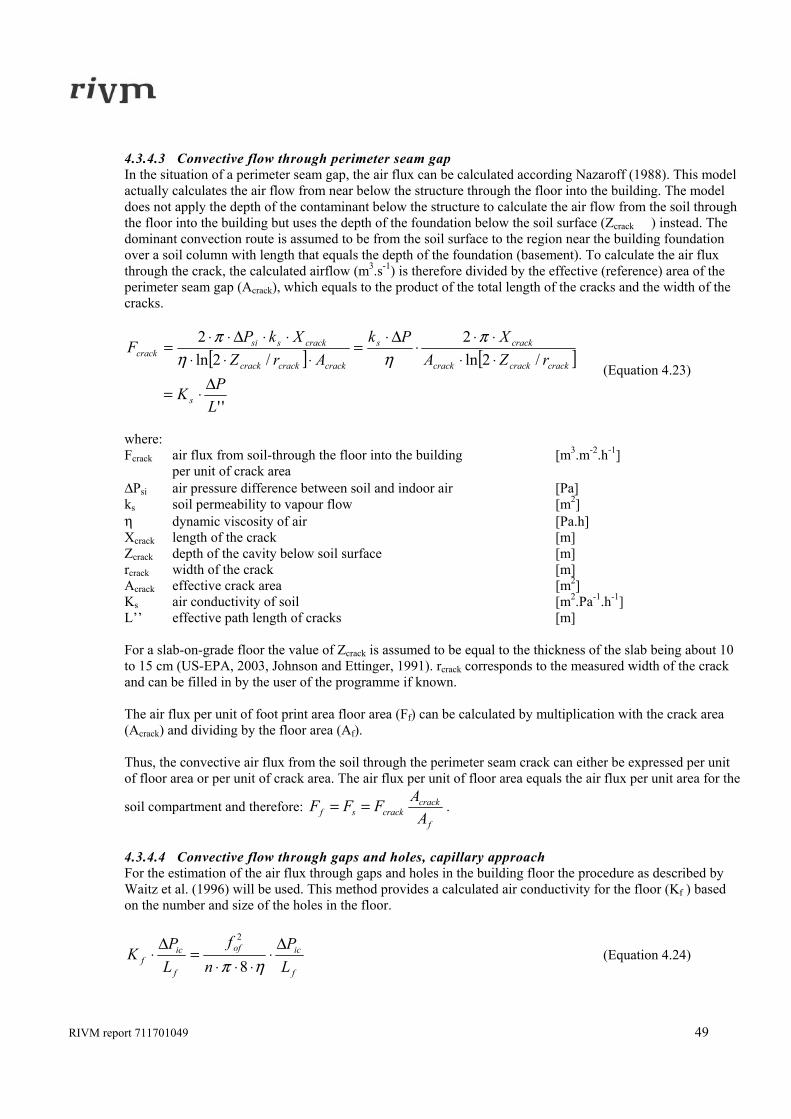
RIVM report 711701049 49
4.3.4.3 Convective flow through perimeter seam gap In the situation of a perimeter seam gap, the air flux can be calculated according Nazaroff (1988). This model actually calculates the air flow from near below the structure through the floor into the building. The model does not apply the depth of the contaminant below the structure to calculate the air flow from the soil through the floor into the building but uses the depth of the foundation below the soil surface (Zcrack ) instead. The dominant convection route is assumed to be from the soil surface to the region near the building foundation over a soil column with length that equals the depth of the foundation (basement). To calculate the air flux through the crack, the calculated airflow (m3.s-1) is therefore divided by the effective (reference) area of the perimeter seam gap (Acrack), which equals to the product of the total length of the cracks and the width of the cracks.
[ ] [ ]
''
/2ln2
/2ln2
LPK
rZAXPk
ArZXkP
F
s
crackcrackcrack
cracks
crackcrackcrack
crackssicrack
Δ⋅=
⋅⋅⋅⋅
⋅Δ⋅
=⋅⋅⋅
⋅⋅Δ⋅⋅=
πηη
π
(Equation 4.23)
where: Fcrack air flux from soil-through the floor into the building [m3.m-2.h-1] per unit of crack area ΔPsi air pressure difference between soil and indoor air [Pa] ks soil permeability to vapour flow [m2] η dynamic viscosity of air [Pa.h] Xcrack length of the crack [m] Zcrack depth of the cavity below soil surface [m] rcrack width of the crack [m] Acrack effective crack area [m2] Ks air conductivity of soil [m2.Pa-1.h-1] L’’ effective path length of cracks [m] For a slab-on-grade floor the value of Zcrack is assumed to be equal to the thickness of the slab being about 10 to 15 cm (US-EPA, 2003, Johnson and Ettinger, 1991). rcrack corresponds to the measured width of the crack and can be filled in by the user of the programme if known. The air flux per unit of foot print area floor area (Ff) can be calculated by multiplication with the crack area (Acrack) and dividing by the floor area (Af). Thus, the convective air flux from the soil through the perimeter seam crack can either be expressed per unit of floor area or per unit of crack area. The air flux per unit of floor area equals the air flux per unit area for the
soil compartment and therefore: f
crackcracksf A
AFFF == .
4.3.4.4 Convective flow through gaps and holes, capillary approach For the estimation of the air flux through gaps and holes in the building floor the procedure as described by Waitz et al. (1996) will be used. This method provides a calculated air conductivity for the floor (Kf ) based on the number and size of the holes in the floor.
f
icof
f
icf L
Pn
fLP
KΔ
⋅⋅⋅⋅
=Δ
⋅ηπ 8
2
(Equation 4.24)
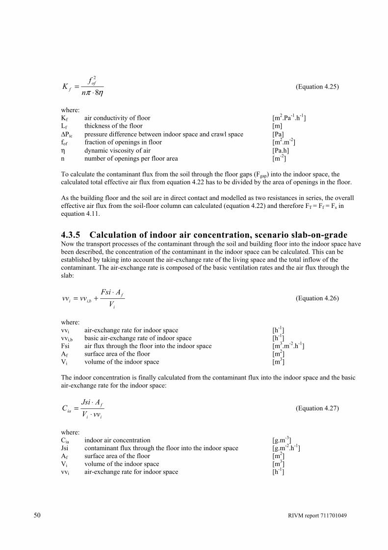
50 RIVM report 711701049
ηπ 8
2
⋅=
nf
K off (Equation 4.25)
where: Kf air conductivity of floor [m2.Pa-1.h-1] Lf thickness of the floor [m] ΔPic pressure difference between indoor space and crawl space [Pa] fof fraction of openings in floor [m2.m-2] η dynamic viscosity of air [Pa.h] n number of openings per floor area [m-2] To calculate the contaminant flux from the soil through the floor gaps (Fgap) into the indoor space, the calculated total effective air flux from equation 4.22 has to be divided by the area of openings in the floor. As the building floor and the soil are in direct contact and modelled as two resistances in series, the overall effective air flux from the soil-floor column can calculated (equation 4.22) and therefore FT = Ff = Fs in equation 4.11.
4.3.5 Calculation of indoor air concentration, scenario slab-on-grade Now the transport processes of the contaminant through the soil and building floor into the indoor space have been described, the concentration of the contaminant in the indoor space can be calculated. This can be established by taking into account the air-exchange rate of the living space and the total inflow of the contaminant. The air-exchange rate is composed of the basic ventilation rates and the air flux through the slab:
i
fbi,i V
AFsivvvv
⋅+= (Equation 4.26)
where: vvi air-exchange rate for indoor space [h-1] vvi,b basic air-exchange rate of indoor space [h-1] Fsi air flux through the floor into the indoor space [m3.m-2.h-1] Af surface area of the floor [m2] Vi volume of the indoor space [m3] The indoor concentration is finally calculated from the contaminant flux into the indoor space and the basic air-exchange rate for the indoor space:
ii
fia vvV
AJsiC
⋅⋅
= (Equation 4.27)
where: Cia indoor air concentration [g.m-3] Jsi contaminant flux through the floor into the indoor space [g.m-2.h-1] Af surface area of the floor [m2] Vi volume of the indoor space [m3] vvi air-exchange rate for indoor space [h-1]
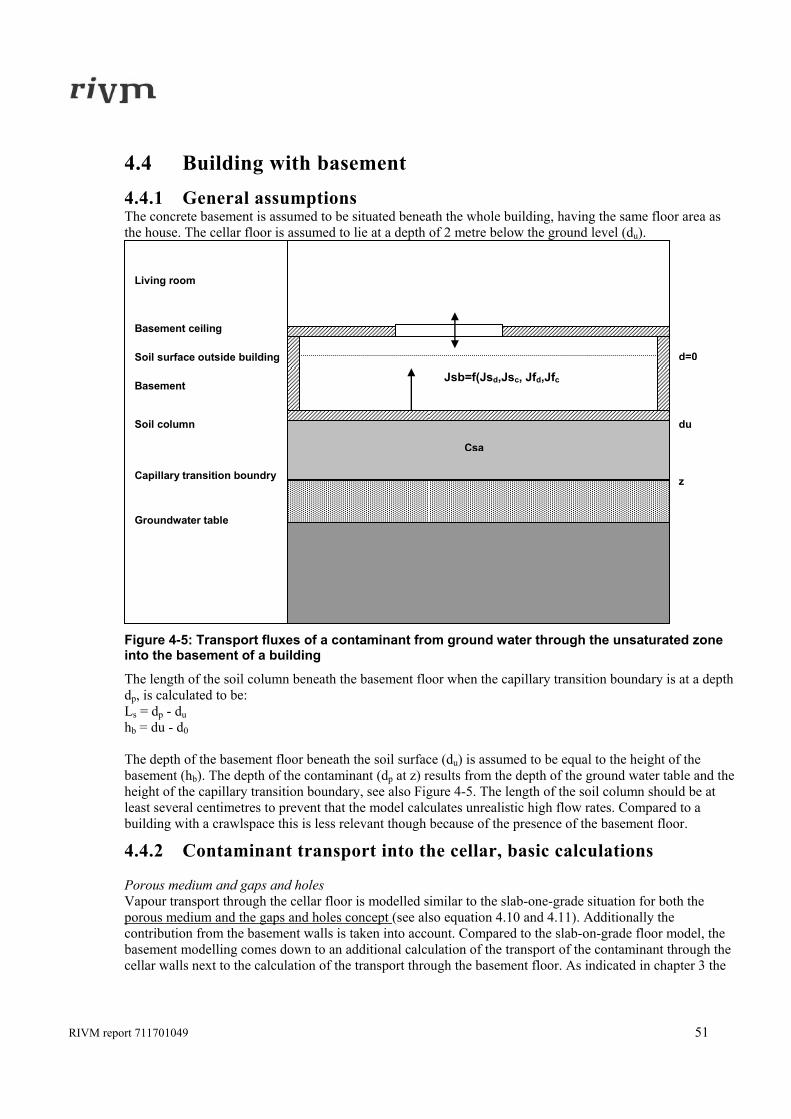
RIVM report 711701049 51
4.4 Building with basement 4.4.1 General assumptions The concrete basement is assumed to be situated beneath the whole building, having the same floor area as the house. The cellar floor is assumed to lie at a depth of 2 metre below the ground level (du).
Groundwater zone
Full capillary zone
Open capillary zone
Boundary layer
Housing floor
Groundwater table
Capillary transition boundry
Soil column
Jsb=f(Jsd,Jsc, Jfd,Jfc
du
z
d=0
Basement
Living room
Basement ceiling
Soil surface outside building
Csa
Figure 4-5: Transport fluxes of a contaminant from ground water through the unsaturated zone into the basement of a building
The length of the soil column beneath the basement floor when the capillary transition boundary is at a depth dp, is calculated to be: Ls = dp - du hb = du - d0 The depth of the basement floor beneath the soil surface (du) is assumed to be equal to the height of the basement (hb). The depth of the contaminant (dp at z) results from the depth of the ground water table and the height of the capillary transition boundary, see also Figure 4-5. The length of the soil column should be at least several centimetres to prevent that the model calculates unrealistic high flow rates. Compared to a building with a crawlspace this is less relevant though because of the presence of the basement floor.
4.4.2 Contaminant transport into the cellar, basic calculations Porous medium and gaps and holes Vapour transport through the cellar floor is modelled similar to the slab-one-grade situation for both the porous medium and the gaps and holes concept (see also equation 4.10 and 4.11). Additionally the contribution from the basement walls is taken into account. Compared to the slab-on-grade floor model, the basement modelling comes down to an additional calculation of the transport of the contaminant through the cellar walls next to the calculation of the transport through the basement floor. As indicated in chapter 3 the
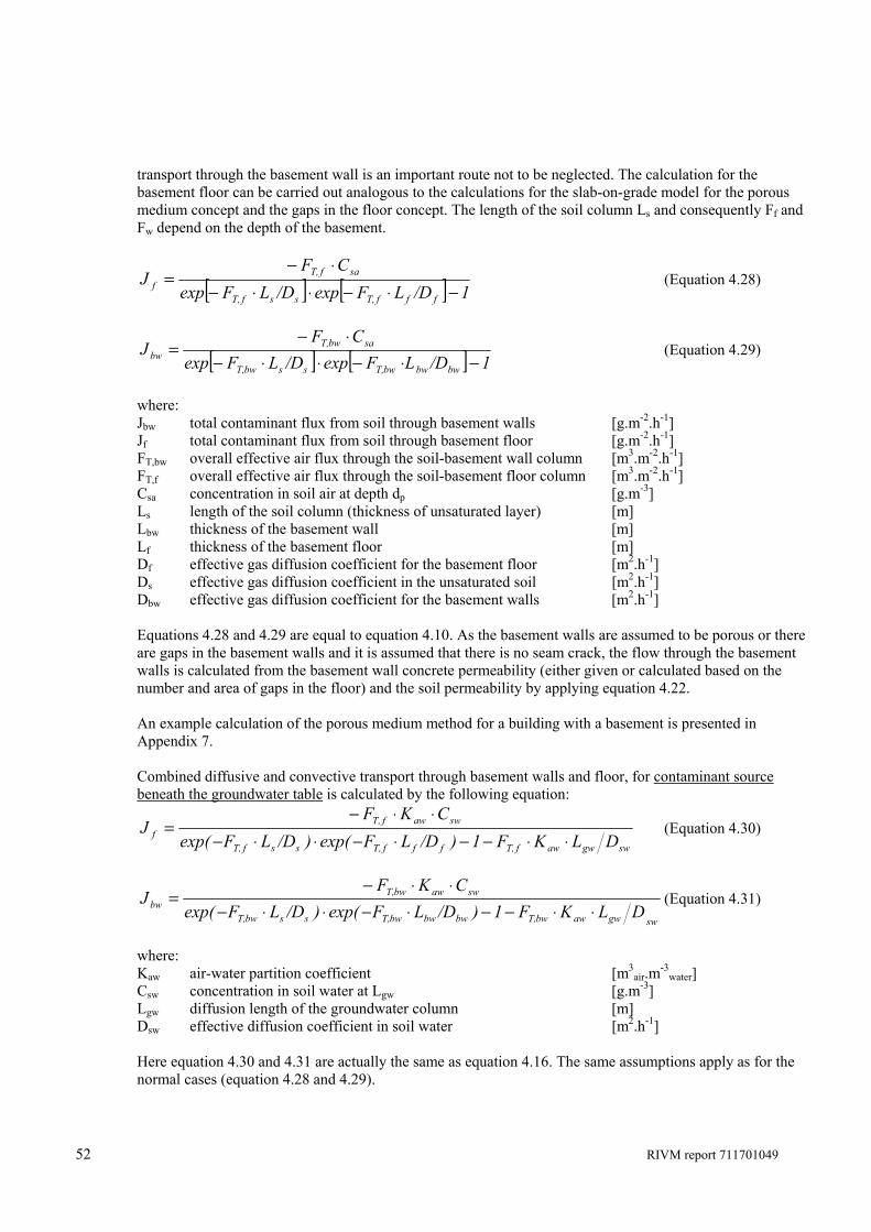
52 RIVM report 711701049
transport through the basement wall is an important route not to be neglected. The calculation for the basement floor can be carried out analogous to the calculations for the slab-on-grade model for the porous medium concept and the gaps in the floor concept. The length of the soil column Ls and consequently Ff and Fw depend on the depth of the basement.
[ ] [ ] 1/DLFexp/DLFexpCF
JfffT,ssfT,
safT,f −⋅−⋅⋅−
⋅−= (Equation 4.28)
[ ] [ ] 1/DLFexp/DLFexpCF
JbwbwbwT,ssbwT,
sabwT,bw −⋅−⋅⋅−
⋅−= (Equation 4.29)
where: Jbw total contaminant flux from soil through basement walls [g.m-2.h-1] Jf total contaminant flux from soil through basement floor [g.m-2.h-1] FT,bw overall effective air flux through the soil-basement wall column [m3.m-2.h-1] FT,f overall effective air flux through the soil-basement floor column [m3.m-2.h-1] Csa concentration in soil air at depth dp [g.m-3] Ls length of the soil column (thickness of unsaturated layer) [m] Lbw thickness of the basement wall [m] Lf thickness of the basement floor [m] Df effective gas diffusion coefficient for the basement floor [m2.h-1] Ds effective gas diffusion coefficient in the unsaturated soil [m2.h-1] Dbw effective gas diffusion coefficient for the basement walls [m2.h-1] Equations 4.28 and 4.29 are equal to equation 4.10. As the basement walls are assumed to be porous or there are gaps in the basement walls and it is assumed that there is no seam crack, the flow through the basement walls is calculated from the basement wall concrete permeability (either given or calculated based on the number and area of gaps in the floor) and the soil permeability by applying equation 4.22. An example calculation of the porous medium method for a building with a basement is presented in Appendix 7. Combined diffusive and convective transport through basement walls and floor, for contaminant source beneath the groundwater table is calculated by the following equation:
swgwawfT,fffT,ssfT,
swawfT,f DLKF1)/DLFexp()/DLFexp(
CKFJ
⋅⋅−−⋅−⋅⋅−⋅⋅−
= (Equation 4.30)
swgwawbwT,bwbwbwT,ssbwT,
swawbwT,bw DLKF1)/DLFexp()/DLFexp(
CKFJ
⋅⋅−−⋅−⋅⋅−⋅⋅−
= (Equation 4.31)
where: Kaw air-water partition coefficient [m3
air.m-3water]
Csw concentration in soil water at Lgw [g.m-3] Lgw diffusion length of the groundwater column [m] Dsw effective diffusion coefficient in soil water [m2.h-1] Here equation 4.30 and 4.31 are actually the same as equation 4.16. The same assumptions apply as for the normal cases (equation 4.28 and 4.29).
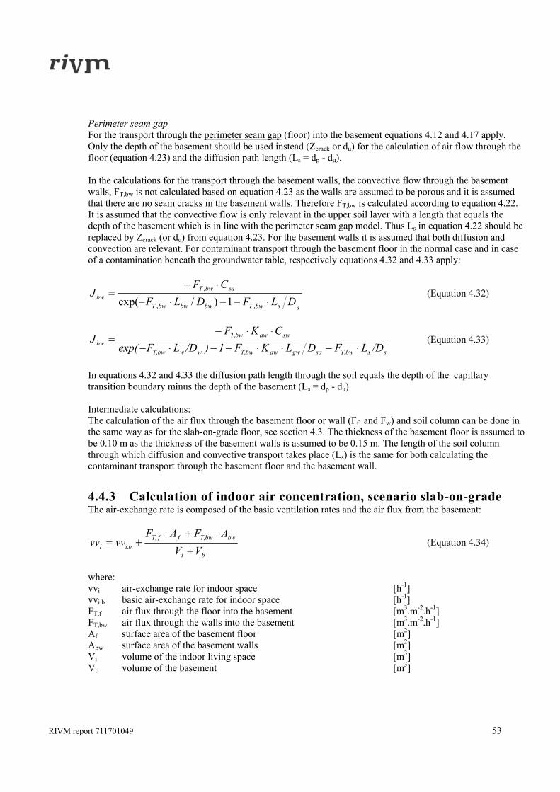
RIVM report 711701049 53
Perimeter seam gap For the transport through the perimeter seam gap (floor) into the basement equations 4.12 and 4.17 apply. Only the depth of the basement should be used instead (Zcrack or du) for the calculation of air flow through the floor (equation 4.23) and the diffusion path length (Ls = dp - du). In the calculations for the transport through the basement walls, the convective flow through the basement walls, FT,bw is not calculated based on equation 4.23 as the walls are assumed to be porous and it is assumed that there are no seam cracks in the basement walls. Therefore FT,bw is calculated according to equation 4.22. It is assumed that the convective flow is only relevant in the upper soil layer with a length that equals the depth of the basement which is in line with the perimeter seam gap model. Thus Ls in equation 4.22 should be replaced by Zcrack (or du) from equation 4.23. For the basement walls it is assumed that both diffusion and convection are relevant. For contaminant transport through the basement floor in the normal case and in case of a contamination beneath the groundwater table, respectively equations 4.32 and 4.33 apply:
ssbwTbwbwbwT
sabwTbw DLFDLF
CFJ
⋅−−⋅−⋅−
=,,
,
1)/exp( (Equation 4.32)
ssbwT,sagwawbwT,wwbwT,
swawbwT,bw /DLFDLKF1)/DLFexp(
CKFJ
⋅−⋅⋅−−⋅−⋅⋅−
= (Equation 4.33)
In equations 4.32 and 4.33 the diffusion path length through the soil equals the depth of the capillary transition boundary minus the depth of the basement (Ls = dp - du). Intermediate calculations: The calculation of the air flux through the basement floor or wall (Ff and Fw) and soil column can be done in the same way as for the slab-on-grade floor, see section 4.3. The thickness of the basement floor is assumed to be 0.10 m as the thickness of the basement walls is assumed to be 0.15 m. The length of the soil column through which diffusion and convective transport takes place (Ls) is the same for both calculating the contaminant transport through the basement floor and the basement wall.
4.4.3 Calculation of indoor air concentration, scenario slab-on-grade The air-exchange rate is composed of the basic ventilation rates and the air flux from the basement:
bi
bwbwT,ffT,bi,i VV
AFAFvvvv
+⋅+⋅
+= (Equation 4.34)
where: vvi air-exchange rate for indoor space [h-1] vvi,b basic air-exchange rate for indoor space [h-1] FT,f air flux through the floor into the basement [m3.m-2.h-1] FT,bw air flux through the walls into the basement [m3.m-2.h-1] Af surface area of the basement floor [m2] Abw surface area of the basement walls [m2] Vi volume of the indoor living space [m3] Vb volume of the basement [m3]
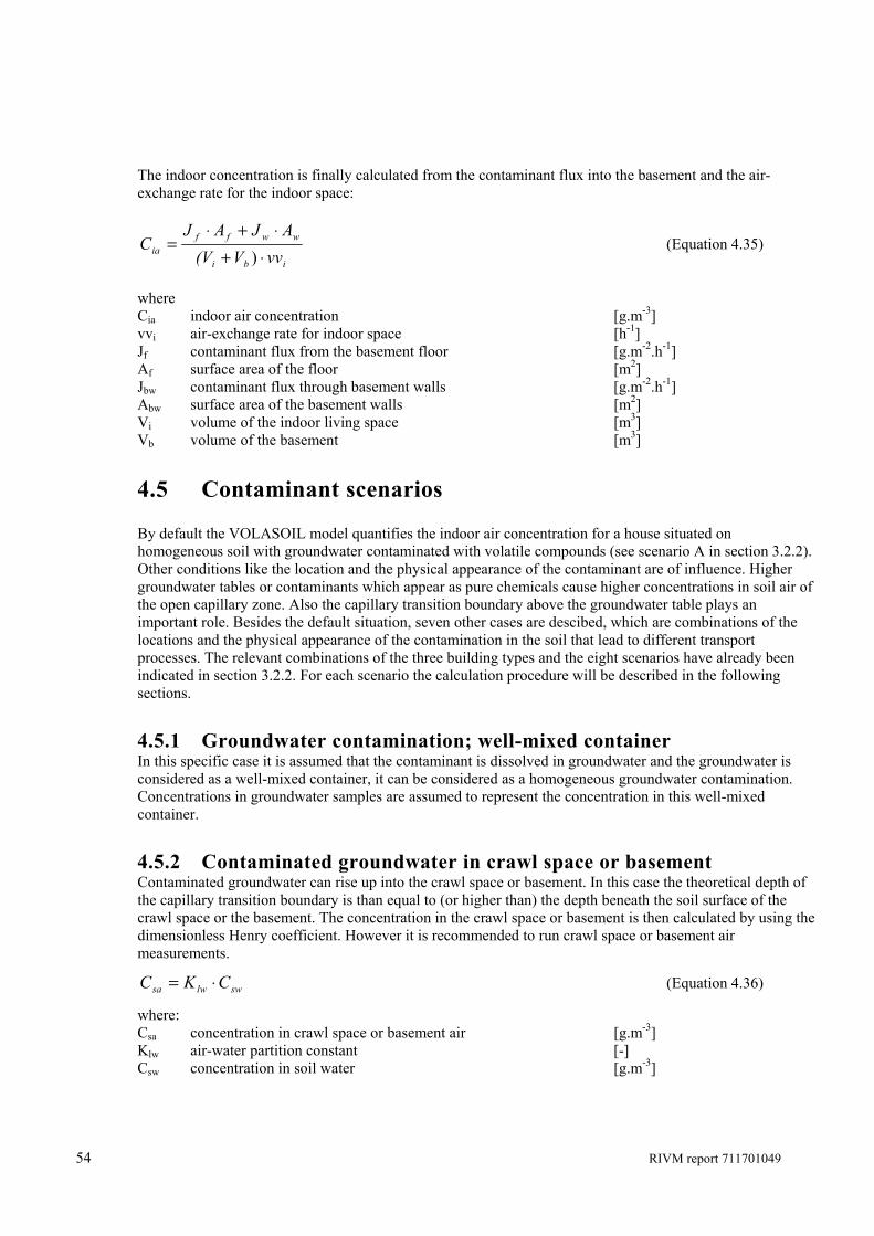
54 RIVM report 711701049
The indoor concentration is finally calculated from the contaminant flux into the basement and the air-exchange rate for the indoor space:
ibi
wwffia vvV(V
AJAJC
⋅+⋅+⋅
=)
(Equation 4.35)
where Cia indoor air concentration [g.m-3] vvi air-exchange rate for indoor space [h-1] Jf contaminant flux from the basement floor [g.m-2.h-1] Af surface area of the floor [m2] Jbw contaminant flux through basement walls [g.m-2.h-1] Abw surface area of the basement walls [m2] Vi volume of the indoor living space [m3] Vb volume of the basement [m3]
4.5 Contaminant scenarios By default the VOLASOIL model quantifies the indoor air concentration for a house situated on homogeneous soil with groundwater contaminated with volatile compounds (see scenario A in section 3.2.2). Other conditions like the location and the physical appearance of the contaminant are of influence. Higher groundwater tables or contaminants which appear as pure chemicals cause higher concentrations in soil air of the open capillary zone. Also the capillary transition boundary above the groundwater table plays an important role. Besides the default situation, seven other cases are descibed, which are combinations of the locations and the physical appearance of the contamination in the soil that lead to different transport processes. The relevant combinations of the three building types and the eight scenarios have already been indicated in section 3.2.2. For each scenario the calculation procedure will be described in the following sections.
4.5.1 Groundwater contamination; well-mixed container In this specific case it is assumed that the contaminant is dissolved in groundwater and the groundwater is considered as a well-mixed container, it can be considered as a homogeneous groundwater contamination. Concentrations in groundwater samples are assumed to represent the concentration in this well-mixed container.
4.5.2 Contaminated groundwater in crawl space or basement Contaminated groundwater can rise up into the crawl space or basement. In this case the theoretical depth of the capillary transition boundary is than equal to (or higher than) the depth beneath the soil surface of the crawl space or the basement. The concentration in the crawl space or basement is then calculated by using the dimensionless Henry coefficient. However it is recommended to run crawl space or basement air measurements.
swlwsa CKC ⋅= (Equation 4.36)
where: Csa concentration in crawl space or basement air [g.m-3] Klw air-water partition constant [-] Csw concentration in soil water [g.m-3]
RIVM report 711701049 55
4.5.3 Floating soil-contaminant layer in the open capillary zone In case of a floating soil-contaminant layer, pure contaminant liquid floats on the groundwater. It is assumed that the floating layer is situated at the capillary transition boundary. At the depth of the capillary fringe, the soil air is saturated with the contaminant, meaning that the soil air concentration can be calculated based on the maximum contamination vapour density.
TRMVpVdCsa ⋅
⋅== (Equation 4.37)
where: Csa concentration in crawl space or basement air [g.m-3] Vd vapour density [g.m-3] Vp vapour pressure [Pa] M molecular weight [g.mol-1] R gas constant [8.314 Pa.m3.mol-1.K-1] T soil temperature [K] 4.5.4 Groundwater in crawl space or basement and a floating soil-contaminant layer A floating soil-contaminant layer exists in combination with a depth of the capillary transition boundary equal to or higher than the depth beneath the soil surface of the crawl space or basement. The concentration in the crawl space or basement is calculated and assumed to be equal to the vapour density.
TRMVpVdCorC baca ⋅
⋅== (Equation 4.38)
where: Cca concentration in crawl space air [g.m-3] Cba concentration in basement air [g.m-3] Vd vapour density [g.m-3] Vp vapour pressure [Pa] M molecular weight [g.mol-1] R gas constant [8.314 Pa.m3.mol-1.K-1] T soil temperature [K]
4.5.5 Pure contaminant in open capillary zone Liquid soil contaminants, which are heavier than water, can be transported as pure product from the soil surface to the groundwater. In the open capillary zone, vertical flow of liquid contaminants can be hampered by relatively impermeable layers of clay, peat and loam. In those cases a pure contaminant layer exists in the open capillary zone. The soil air above this layer is assumed to be saturated with contamination vapours. In case of two or more contaminants the partial vapour pressure should be used to calculate the maximum contaminant vapour density in soil-air as is done for the floating soil contaminant layer in the open capillary zone, see section 4.5.3
56 RIVM report 711701049
4.5.6 Very low groundwater table When a very low groundwater table exists, groundwater concentrations could be difficult to obtain, against high expenses. In this case the concentration in soil air at a certain depth above the groundwater table can be used as input. This concentration can be obtained in two ways, either by soil-air measurements or calculation from the total soil content using equilibrium partitioning. The latter method is described next. The soil-air concentration can be estimated from the total soil concentration by applying equilibrium partitioning, using soil-air partition coefficients. 4.5.7 Sinking soil-contaminant layer In this case the liquid contaminant exists beneath the upper groundwater zone above an aquitarde or aquiclude. Layers of clay, peat and loam are termed aquicludes or when almost impermeable, aquitards. At steady-state conditions, the concentration in groundwater is in equilibrium with the sinking contaminant layer. It is assumed that the concentration in soil water at the capillary transition boundary is equal to the concentration in groundwater, but lower than the concentration in the sinking-contaminant layer. Measured groundwater concentration should be used in order to calculate contaminant fluxes. The average depth is set equal to the depth of the capillary transition boundary in this particular case.
4.5.8 Contaminant source beneath the groundwater table In this case the contaminant source exists beneath the groundwater table, and transport fluxes will be limited. The contaminant transport to the building can be seen as going through two media placed in series. It is assumed that flow of water does not occur and only diffuse transport through the groundwater and full capillary zone is relevant. The elaboration of the calculation procedure is worked out in Appendix 3, see also section 4.3.2.
4.5.9 Estimating the vapour concentration of mixtures For pure contaminant or at low residual levels of contaminants in soil the vapour composition can be assumed to be proportional to the contaminant level in the soil (equilibrium partitioning). Here compounds are sorbed to the soil, dissolved in soil moisture, and present in the vapour space. Contaminants are often not pure, but a mixture of different chemicals like for instance fuels, oils and tars or a mixture of different industrial organic solvents and exist as free phase liquid or precipitate in the soil interstices. In this case of high residual levels of mixtures of contaminants the concentration in soil air is a function of the composition of the contamination. The saturated vapour pressure of a chemical in a mixture is lower compared to that of the pure substance and should be adjusted compared to the vapour pressure of the pure contaminant. The vapour composition can be calculated from the liquid composition according to Raoult’s law. Raoult’s law states that the adjusted vapour pressure of a contaminant in an ideal solution with other contaminants is equal the to mole fraction of the contaminant in this solution times the vapour pressure of the pure contaminant.
FVpVp ⋅=* (Equation 4.39)
where: Vp* true vapour pressure [Pa] Vp vapour pressure [Pa] F mole fraction of chemical in the floating layer [-] For the calculation of the true vapour concentration of a contaminant in soil air, in the crawl space or basement air the exact composition of the contaminant layer should be know in order to calculate the mole fraction. For petrochemical products for instance the composition should be either measured or one might use
RIVM report 711701049 57
standard composition profiles for various petrochemicals products. As an alternative, the mole fraction of a specific chemical can also be determined from the weight averaged molecular weight of the contamination.
i
ai
iiii
ii M
MWMWM
WF
⋅=
⋅=
∑ (Equation 4.40)
where: Fi mole fraction of chemical i in the floating layer [-] Wi mass fraction of chemical i in the floating layer [g.g-1] Mi molecular weight of compound i [g.mol-1] Ma average molecular weight of the floating layer [g.g-1] j index for chemical compound [-] The total number of moles∑
iii MW per unit weight equals the reciproque of the average molecular weight.
The average molecular weights of several petroleum products, which can be present in the sub-soil are listed in Table 4-1.
Table 4-1 The average molecular weight of several petroleum products
Petroleum product Average molecular weight [g.mole-1] References Oil and oil fractions Gasoline 105 1 Jet fuel 165 1 Diesel 230 1 Crude oil 250 2 Lube oil (lube cuts) 355 3 Bitumen (atmospheric cuts) 480 2 Bitumen (vacuum cuts) 970 2 Asphalt 2925 3 Coal tar and coal tar fractions Pitch distillate 170 4 Anthracene oil 178 4 Chrysene fraction 205 4 Coal tar, low 354 5 Coal tar, mid 697 5 Coal tar, high 1950 5 Coal tar pitches 901 6,7 1 US-EPA (2007); 2 Average of European crudes. Data for whole crude and various cuts are from Chevron (2007); 3 Dolomatov (1991). The average of two lube cuts 300-400 °C and 420-500 °C is taken. Asphalt refers to asphaltenes from distillation-cracking petroleum tar; 4 Gilyazetdinov (1992). These are light fractions from coal tar distillation (coal tar oils); 5 Eleven different coal tars have been analysed varying from pure samples to environmental (aged) samples (Brown et al., 2006). The tars have been classified as mid, high or low according to their average molecular weights. The wide range of average molecular weights may result from differences in the manufactured ga process and source material used at the different manufactured gas plants and weathering; 6 Source material is binder pitch used in the production of carbon electrodes for the non-ferrous and ferrous metal production (Hansen et al., 2002); 7 The material analysed is mesophase pitch with an average molecular weight of 910 g/mole (Özel and Bartle, 2001).
58 RIVM report 711701049
This approach of calculating the true vapour pressure is applicable for the situation of a floating soil-contaminant layer in the open capillary zone, a floating soil-contaminant layer in combination with groundwater in the crawl space or basement and when there is a contaminant layer in the open capillary zone.
4.6 Estimating source depletion For long term exposure source depletion and changes in source composition might be relevant. A first-order estimate of whether source depletion is relevant over a certain period of time can be obtained by comparing the mass of the contaminant in the soil to the mass of the contaminant transported from the source into the building. The mass of the contaminant in soil can be calculated from the average (residual) contaminant level in soil and the thickness of the contamination. Furthermore it is assumed that only the area directly beneath the structure is influenced by contaminant transport into the building. The time needed to deplete the contaminant source can be calculated by taking into account the contaminant transport, see equation 4.40
JLC
AfJAfLC
t lblllbll ⋅⋅=
⋅⋅⋅⋅
= ,, ρρ (Equation 4.41)
where: t time needed to deplete the contaminant source [h] ρl bulk density of the contamination layer [kg.m-3] Cl,b average (bulk) concentration in the contamination layer [kg.kgsoil
-1] Ll thickness of the contamination layer in soil [m] Af floor area [m2] J contaminant flux into the building [g.m-2.h-1]
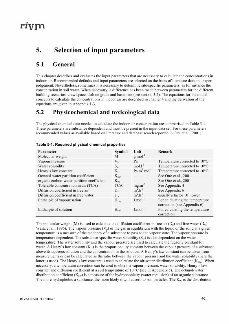
RIVM report 711701049 59
5. Selection of input parameters
5.1 General This chapter describes and evaluates the input parameters that are necessary to calculate the concentrations in indoor air. Recommended defaults and input parameters are selected on the basis of literature data and expert judgement. Nevertheless, sometimes it is necessary to determine site-specific parameters, as for instance the concentration in soil water. When necessary, a difference has been made between parameters for the different building scenarios: crawlspace, slab on grade and basement (see section 3.2). The equations for the model concepts to calculate the concentrations in indoor air are described in chapter 4 and the derivation of the equations are given in Appendix 1-3.
5.2 Physicochemical and toxicological data The physical chemical data needed to calculate the indoor air concentration are summarised in Table 5-1. These parameters are substance dependent and must be present in the input data set. For these parameters recommended values ar available based on literature and database search reported in Otte et al. (2001).
Table 5-1: Required physical chemical properties
Parameter Symbol Unit Remark Molecular weight M g.mol-1 Vapour Pressure Vp Pa Temperature corrected to 10°C Water solubility Sw mol.l-1 Temperature corrected to 10°C Henry’s law constant KH Pa.m3.mol-1 Temperature corrected to 10°C Octanol-water partition coefficient Kow - See Otte et al., 2001 organic carbon-water partition coefficient Koc - See Otte et al., 2001 Tolerable concentration in air (TCA) TCA mg.m-3 See Appendix 4 Diffusion coefficient in free air Da m2.h-1 See Appendix 6 Diffusion coefficient in free water Dw m2.h-1 usually a factor 104 lower Enthalpie of vapourisation Hvap J.mol-1 For calculating the temperature
correction (see Appendix 6) Enthalpie of solution Hsol J.mol-1 For calculating the temperature
correction The molecular weight (M) is used to calculate the diffusion coefficient in free air (Da) and free water (Dw) Waitz et al., 1996). The vapour pressure (Vp) of the gas in equilibrium with the liquid or the solid at a given temperature is a measure of the tendency of a substance to pass to the vapour state. The vapour pressure is temperature dependent. The substance-specific water solubility (Sw) is also dependent on the water temperature. The water solubility and the vapour pressure are used to calculate the fugacity constant for water. A Henry’s law constant (KH) is the proportionality constant between the vapour pressure of a substance above its aqueous solution and the concentration in the solution. A Henry’s law constant can be taken from measurements or can be calculated as the ratio between the vapour pressure and the water solubility (here the latter is used). The Henry’s law constant is used to calculate the air-water distribution coefficient (Kaw). When necessary, a temperature correction can be used to obtain a vapour pressure, water solubility, Henry’s law constant and diffusion coefficient at a soil temperature of 10 °C (see in Appendix 5). The octanol-water distribution coefficient (Kow) is a measure of the hydrophobicity (water repulsion) of an organic substance. The more hydrophobic a substance, the more likely it will adsorb to soil particles. The Koc is the distribution
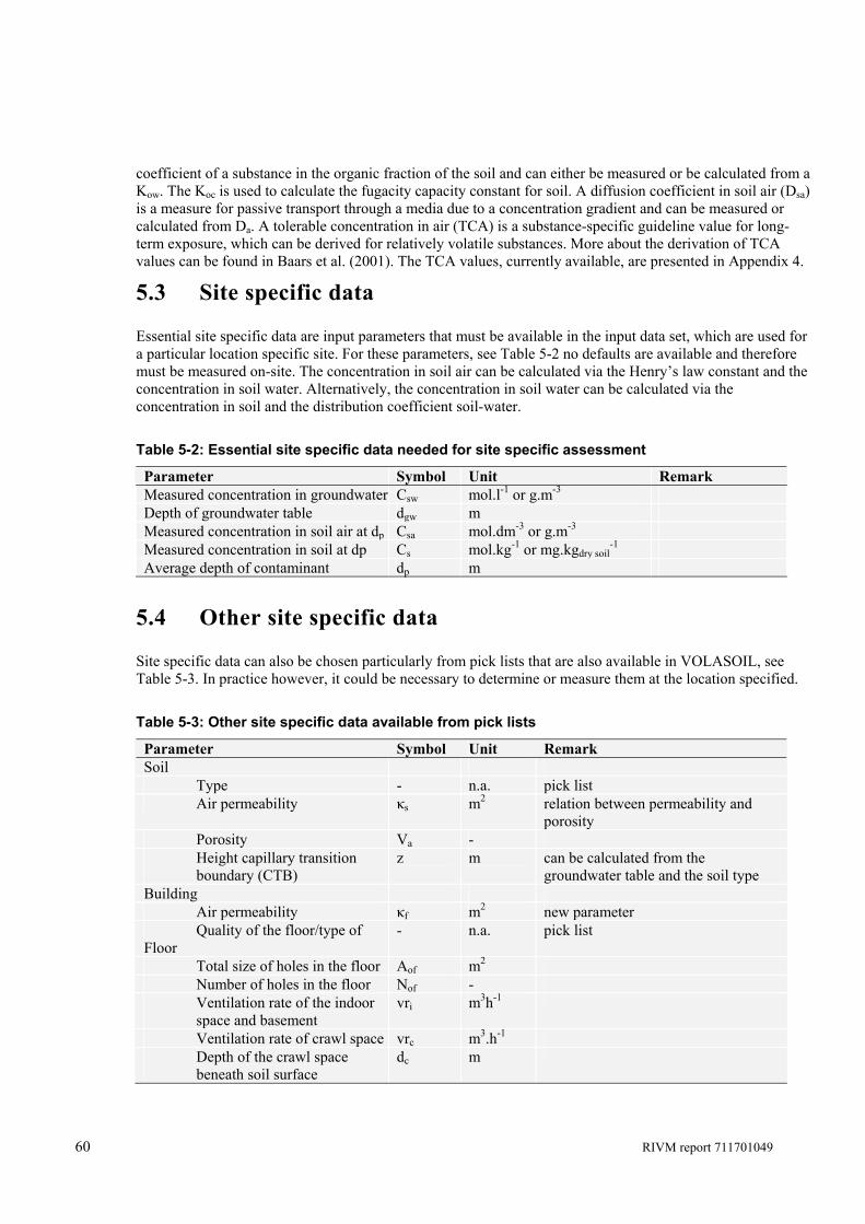
60 RIVM report 711701049
coefficient of a substance in the organic fraction of the soil and can either be measured or be calculated from a Kow. The Koc is used to calculate the fugacity capacity constant for soil. A diffusion coefficient in soil air (Dsa) is a measure for passive transport through a media due to a concentration gradient and can be measured or calculated from Da. A tolerable concentration in air (TCA) is a substance-specific guideline value for long-term exposure, which can be derived for relatively volatile substances. More about the derivation of TCA values can be found in Baars et al. (2001). The TCA values, currently available, are presented in Appendix 4.
5.3 Site specific data Essential site specific data are input parameters that must be available in the input data set, which are used for a particular location specific site. For these parameters, see Table 5-2 no defaults are available and therefore must be measured on-site. The concentration in soil air can be calculated via the Henry’s law constant and the concentration in soil water. Alternatively, the concentration in soil water can be calculated via the concentration in soil and the distribution coefficient soil-water.
Table 5-2: Essential site specific data needed for site specific assessment
Parameter Symbol Unit Remark Measured concentration in groundwater Csw mol.l-1 or g.m-3 Depth of groundwater table dgw m Measured concentration in soil air at dp Csa mol.dm-3 or g.m-3 Measured concentration in soil at dp Cs mol.kg-1 or mg.kgdry soil
-1 Average depth of contaminant dp m
5.4 Other site specific data Site specific data can also be chosen particularly from pick lists that are also available in VOLASOIL, see Table 5-3. In practice however, it could be necessary to determine or measure them at the location specified.
Table 5-3: Other site specific data available from pick lists
Parameter Symbol Unit Remark Soil Type - n.a. pick list Air permeability κs m2 relation between permeability and
porosity Porosity Va - Height capillary transition boundary (CTB)
z m can be calculated from the groundwater table and the soil type
Building Air permeability κf m2 new parameter Quality of the floor/type of Floor
- n.a. pick list
Total size of holes in the floor Aof m2 Number of holes in the floor Nof - Ventilation rate of the indoor space and basement
vri m3h-1
Ventilation rate of crawl space vrc m3.h-1 Depth of the crawl space beneath soil surface
dc m
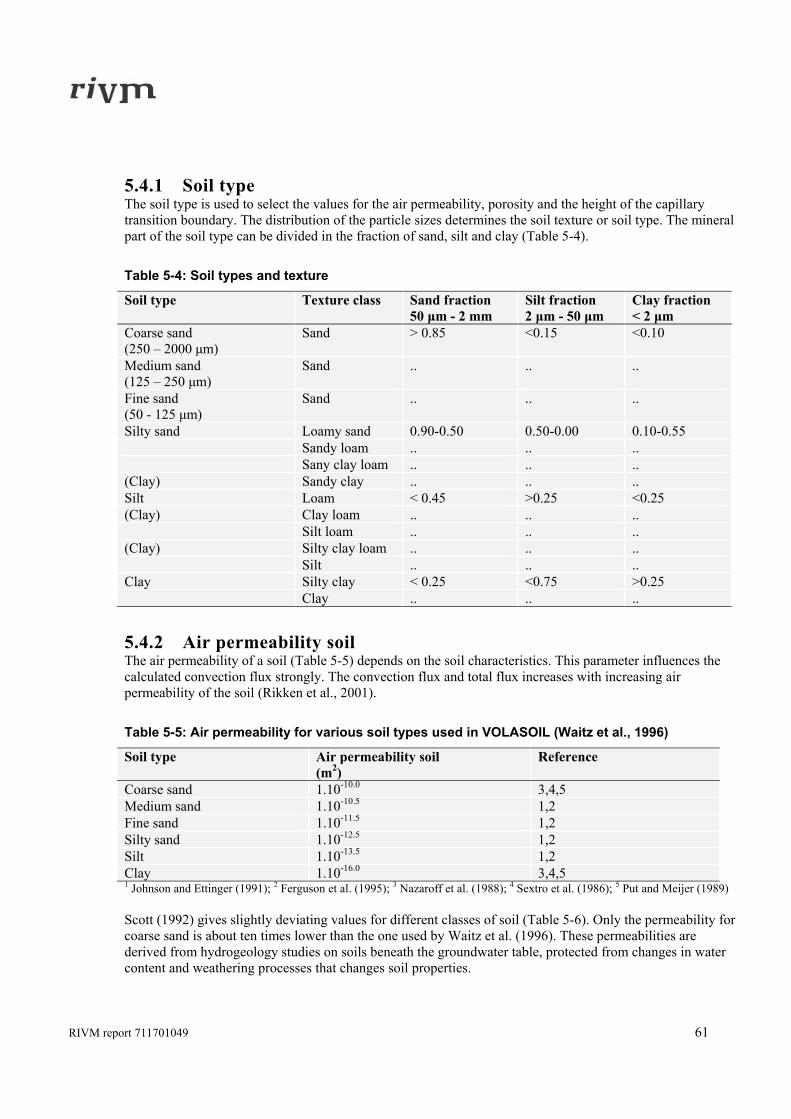
RIVM report 711701049 61
5.4.1 Soil type The soil type is used to select the values for the air permeability, porosity and the height of the capillary transition boundary. The distribution of the particle sizes determines the soil texture or soil type. The mineral part of the soil type can be divided in the fraction of sand, silt and clay (Table 5-4).
Table 5-4: Soil types and texture
Soil type Texture class Sand fraction 50 μm - 2 mm
Silt fraction 2 μm - 50 μm
Clay fraction < 2 μm
Coarse sand (250 – 2000 μm)
Sand > 0.85 <0.15 <0.10
Medium sand (125 – 250 μm)
Sand .. .. ..
Fine sand (50 - 125 μm)
Sand .. .. ..
Silty sand Loamy sand 0.90-0.50 0.50-0.00 0.10-0.55 Sandy loam .. .. .. Sany clay loam .. .. .. (Clay) Sandy clay .. .. .. Silt Loam < 0.45 >0.25 <0.25 (Clay) Clay loam .. .. .. Silt loam .. .. .. (Clay) Silty clay loam .. .. .. Silt .. .. .. Clay Silty clay < 0.25 <0.75 >0.25 Clay .. .. ..
5.4.2 Air permeability soil The air permeability of a soil (Table 5-5) depends on the soil characteristics. This parameter influences the calculated convection flux strongly. The convection flux and total flux increases with increasing air permeability of the soil (Rikken et al., 2001).
Table 5-5: Air permeability for various soil types used in VOLASOIL (Waitz et al., 1996)
Soil type Air permeability soil (m2)
Reference
Coarse sand 1.10-10.0 3,4,5 Medium sand 1.10-10.5 1,2 Fine sand 1.10-11.5 1,2 Silty sand 1.10-12.5 1,2 Silt 1.10-13.5 1,2 Clay 1.10-16.0 3,4,5 1 Johnson and Ettinger (1991); 2 Ferguson et al. (1995); 3 Nazaroff et al. (1988); 4 Sextro et al. (1986); 5 Put and Meijer (1989) Scott (1992) gives slightly deviating values for different classes of soil (Table 5-6). Only the permeability for coarse sand is about ten times lower than the one used by Waitz et al. (1996). These permeabilities are derived from hydrogeology studies on soils beneath the groundwater table, protected from changes in water content and weathering processes that changes soil properties.
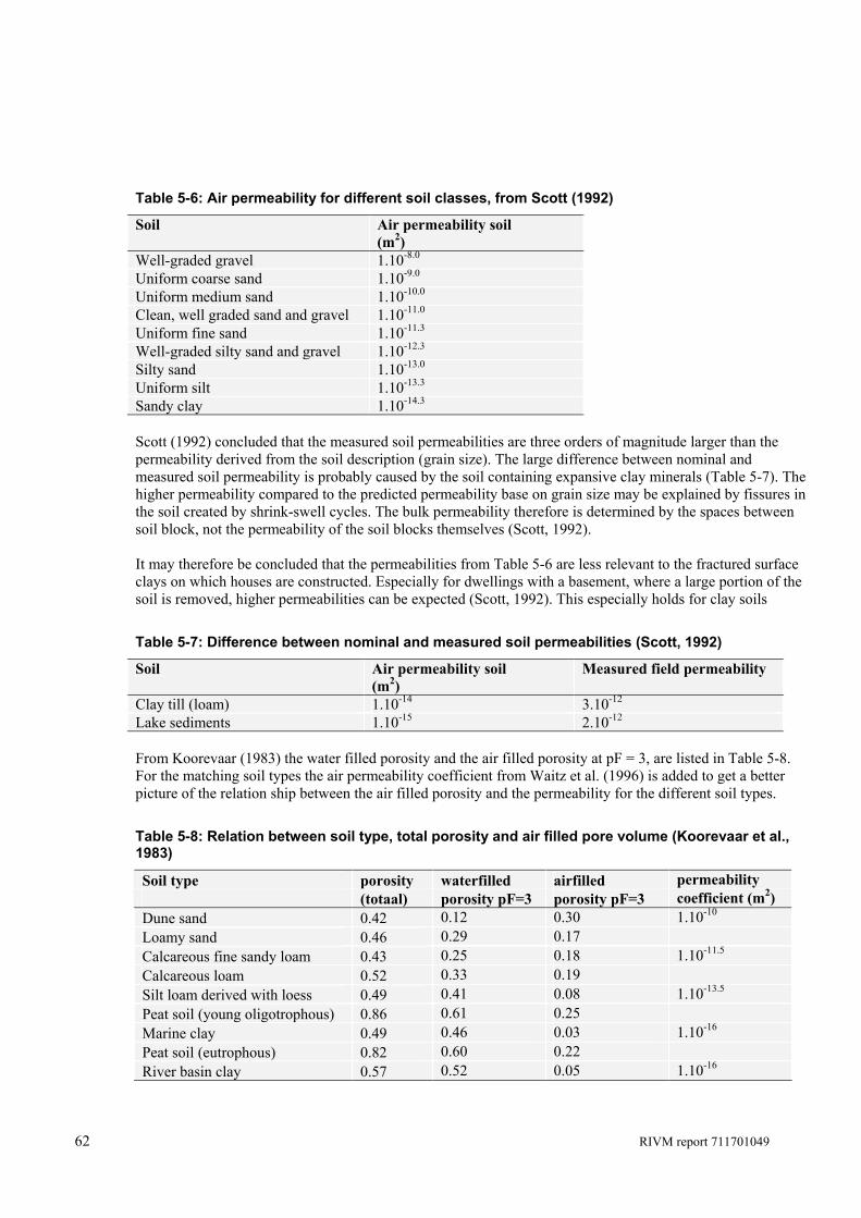
62 RIVM report 711701049
Table 5-6: Air permeability for different soil classes, from Scott (1992)
Soil Air permeability soil (m2)
Well-graded gravel 1.10-8.0
Uniform coarse sand 1.10-9.0 Uniform medium sand 1.10-10.0 Clean, well graded sand and gravel 1.10-11.0 Uniform fine sand 1.10-11.3 Well-graded silty sand and gravel 1.10-12.3 Silty sand 1.10-13.0 Uniform silt 1.10-13.3 Sandy clay 1.10-14.3 Scott (1992) concluded that the measured soil permeabilities are three orders of magnitude larger than the permeability derived from the soil description (grain size). The large difference between nominal and measured soil permeability is probably caused by the soil containing expansive clay minerals (Table 5-7). The higher permeability compared to the predicted permeability base on grain size may be explained by fissures in the soil created by shrink-swell cycles. The bulk permeability therefore is determined by the spaces between soil block, not the permeability of the soil blocks themselves (Scott, 1992). It may therefore be concluded that the permeabilities from Table 5-6 are less relevant to the fractured surface clays on which houses are constructed. Especially for dwellings with a basement, where a large portion of the soil is removed, higher permeabilities can be expected (Scott, 1992). This especially holds for clay soils
Table 5-7: Difference between nominal and measured soil permeabilities (Scott, 1992)
Soil Air permeability soil (m2)
Measured field permeability
Clay till (loam) 1.10-14 3.10-12 Lake sediments 1.10-15 2.10-12 From Koorevaar (1983) the water filled porosity and the air filled porosity at pF = 3, are listed in Table 5-8. For the matching soil types the air permeability coefficient from Waitz et al. (1996) is added to get a better picture of the relation ship between the air filled porosity and the permeability for the different soil types.
Table 5-8: Relation between soil type, total porosity and air filled pore volume (Koorevaar et al., 1983)
Soil type porosity waterfilled airfilled permeability (totaal) porosity pF=3 porosity pF=3 coefficient (m2) Dune sand 0.42 0.12 0.30 1.10-10 Loamy sand 0.46 0.29 0.17 Calcareous fine sandy loam 0.43 0.25 0.18 1.10-11.5 Calcareous loam 0.52 0.33 0.19 Silt loam derived with loess 0.49 0.41 0.08 1.10-13.5 Peat soil (young oligotrophous) 0.86 0.61 0.25 Marine clay 0.49 0.46 0.03 1.10-16 Peat soil (eutrophous) 0.82 0.60 0.22 River basin clay 0.57 0.52 0.05 1.10-16
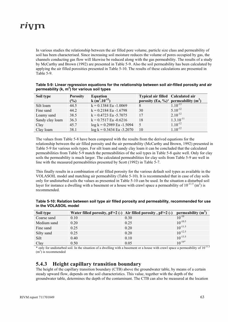
RIVM report 711701049 63
In various studies the relationship between the air filled pore volume, particle size class and permeability of soil has been characterised. Since increasing soil moisture reduces the volume of pores occupied by gas, the channels conducting gas flow will likewise be reduced along with the gas permeability. The results of a study by McCarthy and Brown (1992) are presented in Table 5-9. Also the soil permeability has been calculated by applying the air filled porosities presented in Table 5-10. The results of these calculations are presented in Table 5-9.
Table 5-9: Linear regression equations for the relationship between soil air-filled porosity and air permeability (k, m2) for various soil types
Soil type Porosity (%)
Equation k (m2.10-12)
Typical air filled porosity (Ea, %)*
Calculated air permeability (m2)
Silt loam 44.5 k = 0.1384 Ea -1.0069 8 1.10-13
Fine sand 44.2 k = 0.2184 Ea -1.6798 30 5.10-12 Loamy sand 38.5 k = 0.4723 Ea -5.7075 17 2.10-12 Sandy clay loam 36.3 k = 0.7517 Ea -0.6216 18 1.3.10-11 Clay 45.7 log k = 0.2989 Ea -1.5094 5 1.10-12 Clay loam 38.1 log k = 0.3434 Ea -3.2070 10 1.10-12 The values from Table 5-8 have been compared with the results from the derived equations for the relationship between the air filled porosity and the air permeability (McCarthy and Brown, 1992) presented in Table 5-9 for various soils types. For silt loam and sandy clay loam it can be concluded that the calculated permeabilities from Table 5-9 match the permeabilities of the soil types in Table 5-8 quite well. Only for clay soils the permeability is much larger. The calculated permeabilities for clay soils from Table 5-9 are well in line with the measured permeabilities presented by Scott (1992) in Table 5-7. This finally results in a combination of air filled porosity for the various default soil types as available in the VOLASOIL model and matching air permeability (Table 5-10). It is recommended that in case of clay soils only for undisturbed soils the values as presented in Table 5-10 can be used. In the situation a disturbed soil layer for instance a dwelling with a basement or a house with crawl space a permeability of 10-11.5 (m2) is recommended.
Table 5-10: Relation between soil type air filled porosity and permeability, recommended for use in the VOLASOIL model
Soil type Water filled porosity, pF=2 (-) Air filled porosity , pF=2 (-) permeability (m2) Coarse sand 0.10 0.30 10-10 Medium sand 0.20 0.25 10-10.5 Fine sand 0.25 0.20 10-11.5 Silty sand 0.25 0.20 10-12.5 Silt 0.40 0.10 10-13.5 Clay 0.50 0.05 10-16* * only for undisturbed soil. In the situation of a dwelling with a basement or a house with crawl space a permeability of 10-11.5 (m2) is recommended
5.4.3 Height capillary transition boundary The height of the capillary transition boundary (CTB) above the groundwater table, by means of a certain steady upward flow, depends on the soil characteristics. This value, together with the depth of the groundwater table, determines the depth of the contaminant. The CTB can also be measured at the location
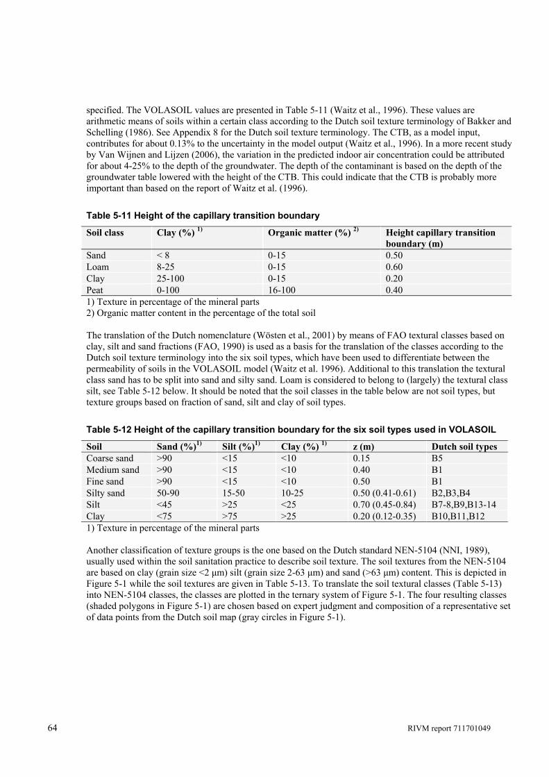
64 RIVM report 711701049
specified. The VOLASOIL values are presented in Table 5-11 (Waitz et al., 1996). These values are arithmetic means of soils within a certain class according to the Dutch soil texture terminology of Bakker and Schelling (1986). See Appendix 8 for the Dutch soil texture terminology. The CTB, as a model input, contributes for about 0.13% to the uncertainty in the model output (Waitz et al., 1996). In a more recent study by Van Wijnen and Lijzen (2006), the variation in the predicted indoor air concentration could be attributed for about 4-25% to the depth of the groundwater. The depth of the contaminant is based on the depth of the groundwater table lowered with the height of the CTB. This could indicate that the CTB is probably more important than based on the report of Waitz et al. (1996).
Table 5-11 Height of the capillary transition boundary
Soil class Clay (%) 1) Organic matter (%) 2) Height capillary transition boundary (m)
Sand < 8 0-15 0.50 Loam 8-25 0-15 0.60 Clay 25-100 0-15 0.20 Peat 0-100 16-100 0.40 1) Texture in percentage of the mineral parts 2) Organic matter content in the percentage of the total soil The translation of the Dutch nomenclature (Wösten et al., 2001) by means of FAO textural classes based on clay, silt and sand fractions (FAO, 1990) is used as a basis for the translation of the classes according to the Dutch soil texture terminology into the six soil types, which have been used to differentiate between the permeability of soils in the VOLASOIL model (Waitz et al. 1996). Additional to this translation the textural class sand has to be split into sand and silty sand. Loam is considered to belong to (largely) the textural class silt, see Table 5-12 below. It should be noted that the soil classes in the table below are not soil types, but texture groups based on fraction of sand, silt and clay of soil types.
Table 5-12 Height of the capillary transition boundary for the six soil types used in VOLASOIL
Soil Sand (%)1) Silt (%)1) Clay (%) 1) z (m) Dutch soil types Coarse sand >90 <15 <10 0.15 B5 Medium sand >90 <15 <10 0.40 B1 Fine sand >90 <15 <10 0.50 B1 Silty sand 50-90 15-50 10-25 0.50 (0.41-0.61) B2,B3,B4 Silt <45 >25 <25 0.70 (0.45-0.84) B7-8,B9,B13-14 Clay <75 >75 >25 0.20 (0.12-0.35) B10,B11,B12 1) Texture in percentage of the mineral parts Another classification of texture groups is the one based on the Dutch standard NEN-5104 (NNI, 1989), usually used within the soil sanitation practice to describe soil texture. The soil textures from the NEN-5104 are based on clay (grain size <2 μm) silt (grain size 2-63 μm) and sand (>63 μm) content. This is depicted in Figure 5-1 while the soil textures are given in Table 5-13. To translate the soil textural classes (Table 5-13) into NEN-5104 classes, the classes are plotted in the ternary system of Figure 5-1. The four resulting classes (shaded polygons in Figure 5-1) are chosen based on expert judgment and composition of a representative set of data points from the Dutch soil map (gray circles in Figure 5-1).
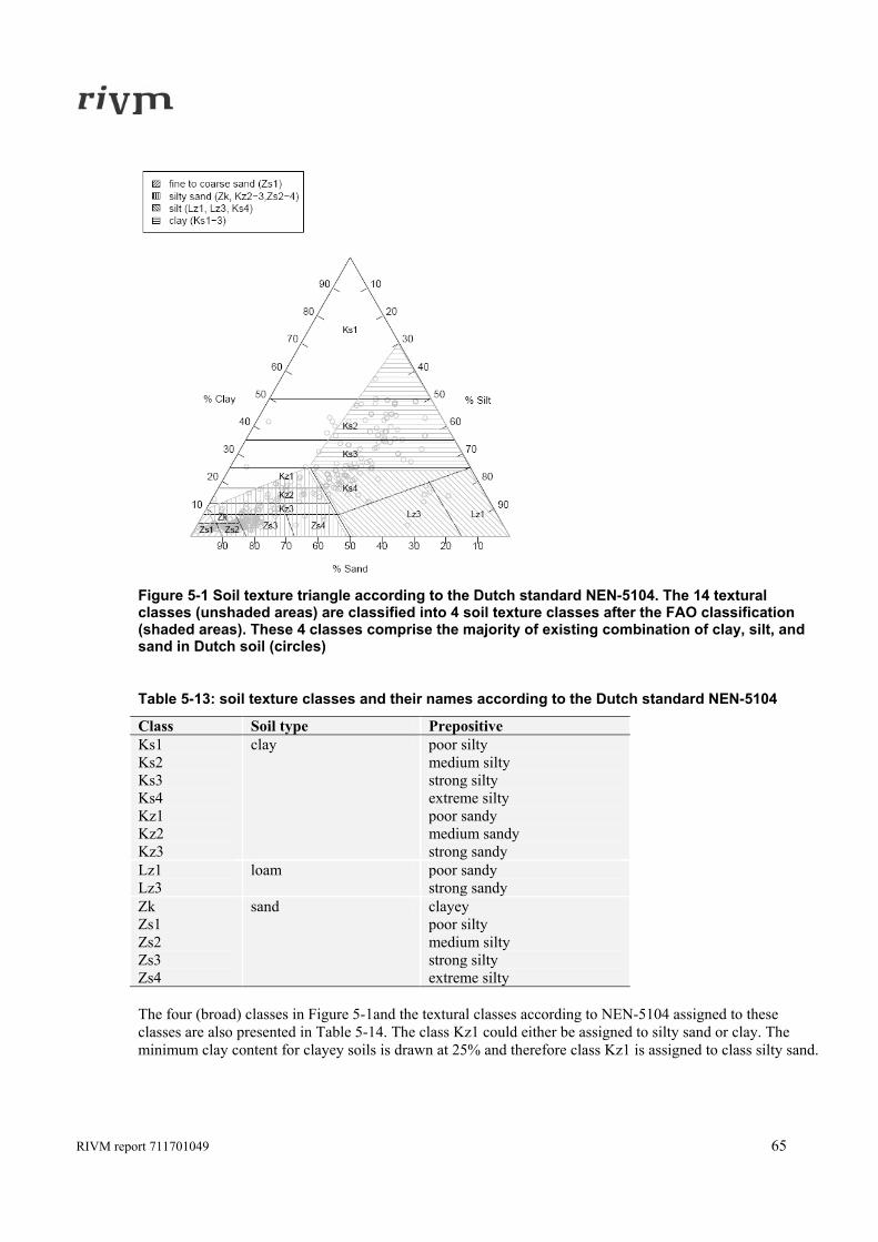
RIVM report 711701049 65
Figure 5-1 Soil texture triangle according to the Dutch standard NEN-5104. The 14 textural classes (unshaded areas) are classified into 4 soil texture classes after the FAO classification (shaded areas). These 4 classes comprise the majority of existing combination of clay, silt, and sand in Dutch soil (circles)
Table 5-13: soil texture classes and their names according to the Dutch standard NEN-5104
Class Soil type Prepositive Ks1 Ks2 Ks3 Ks4 Kz1 Kz2 Kz3
clay poor silty medium silty strong silty extreme silty poor sandy medium sandy strong sandy
Lz1 Lz3
loam poor sandy strong sandy
Zk Zs1 Zs2 Zs3 Zs4
sand clayey poor silty medium silty strong silty extreme silty
The four (broad) classes in Figure 5-1and the textural classes according to NEN-5104 assigned to these classes are also presented in Table 5-14. The class Kz1 could either be assigned to silty sand or clay. The minimum clay content for clayey soils is drawn at 25% and therefore class Kz1 is assigned to class silty sand.
66 RIVM report 711701049
Table 5-14 Translation of the Dutch soil types and soil texture classes according to NEN- 5104 into the six broad soil types used in the VOLASOIL model
Soil Sand (%)1) Silt (%)1) Clay (%) 1) Dutch soil types NEN 5104 Coarse sand >90 <15 <10 B5 Zs1 Medium sand >90 <15 <10 B1 Zs1 Fine sand >90 <15 <10 B1 Zs1 Silty sand 50-90 15-50 10-25 B2,B3,B4 Zk, Kz1-3, Zs2-4 Silt <45 >25 <25 B7-8,B9,B13-14 Lz1, Lz3, Ks4 Clay <75 >75 >25 B10,B11,B12 Ks1-3 1 Texture in percentage of the mineral parts
5.4.4 Quality of the floor The air flux through the floor to indoor air occurs through gaps, cracks and holes in the floor. The quality of the floor is expressed in terms of the total area of openings in the floor or the fraction of openings in the floor (Table 5-15). The air exchange rate of a crawling space depends also on the quality of the floor. The quality of the floor can be good, normal or bad (Waitz et al., 1996).
Table 5-15 Floor quality as used in VOLASOIL (Waitz et al., 1996)
Quality of floor Total area of openings in floor (m2) Fraction of openings in floor (m2/m2) Bad (default) 0.005 0.0001 Normal 0.0005 0.00001 Good 0.00005 0.000001 The leakage area of the ground floor for newly built dwellings and an old dwelling type without concrete construction elements is reported by Janssen et al. (1998). The leakage area of the ground floor for newly built dwellings (1985-1993) with concrete elements ranges from 18 to 71 cm2. The leakage area for the older (early sixties) building type with a wooden floor and brick walls, is reported to be 240 cm2 (Table 5-16). The total leakage area in ground floors in the Netherlands is said to generally vary between 6 and 200 cm2. To express the floor quality, the fraction of openings in the floor is used in the VOLASOIL model. To do the same for the data reported by Janssen et al. (1998) a floor plan of 41m2 is used as an average for the Netherlands (Janssen et al., 1998). The results are listed in Table 5-16.
Table 5-16 Leakage area of the ground floor for different types of buildings
Dwelling type Total area of openings in floor (m2) Fraction of openings in floor (m2/m2) N1 0.0018 0.00004 N2 0.0034 0.00008 N3 0.0071 0.00017 N4 0.0056 0.00014 O 0.0240 0.00058 The fraction of openings in the ground floor, as reported by Janssen et al. (1998), are about the value for the bad floor quality type as used in the VOLASOIL model (Waitz et al., 1996). The use of the bad floor quality type as the default seems to be justified, considering the values as reported by Janssen et al. (1998). From this experimental data it can also be concluded that a normal quality of the floor is rather good actually. An additional floor quality type might be considered for wooden floors. At these high values for the leakage area of about 0.025 m2 and at constant building depressurisation of about 1 to 2 Pascal, the air flow rate into the indoor building space and the contaminant inflow would be high. It is expected that at these high inflow rates the building depressurization would be lower. For this reason the total leakage area for a wooden floor is set at 0.0002 m2.m-2. This results in a total area of openings for the VOLASOIL model of 0.010 m2.
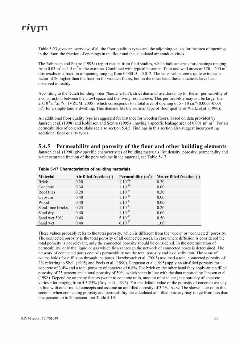
RIVM report 711701049 67
Table 5-23 gives an overview of all the floor qualities types and the adjoining values for the area of openings in the floor, the fraction of openings in the floor and the calculated air conductivities. The Robinson and Sextro (1995a) report results from field studies, which indicate areas for openings ranging from 0.03 m2 to 1.5 m2 in the extreme. Combined with typical basement floor and wall areas of 120 – 200 m2 this results in a fraction of opening ranging from 0.00015 – 0.012. The latter value seems quite extreme, a factor of 20 higher than the fraction for wooden floors, but on the other hand these situations have been observed in reality. According to the Dutch building order ('bouwbesluit'), strict demands are drawn up for the air permeability of a construction between the crawl space and the living room above. This permeability may not be larger than 20.10-6 m3.m-2s-1 (VROM, 2005), which corresponds to a total area of opening of 5 - 10 cm2 (0.0005-0.001 m2) for a single-family dwelling. This demand fits the 'normal' type of floor quality of Waitz et al. (1996). An additional floor quality type is suggested for instance for wooden floors, based on data provided by Janssen et al. (1998) and Robinson and Sextro (1995a), having a specific leakage area of 0.001 m2.m-2. For air permeabilities of concrete slabs see also section 5.4.5. Findings in this section also suggest incorporating additional floor quality types.
5.4.5 Permeability and porosity of the floor and other building elements Janssen et al. (1998) give specific characteristics of building materials like density, porosity, permeability and water saturated fraction of the pore volume in the material, see Table 5-17.
Table 5-17 Characteristics of building materials
Material Air filled fraction (-) Permeability (m2) Water filled fraction (-) Brick 0.20 1.10-14 0.30 Concrete 0.30 1.10-16 0.00 Roof tiles 0.20 1.10-14 0.30 Gypsum 0.40 1.10-13 0.00 Wood 0.40 1.10-13 0.00 Sand-lime bricks 0.24 1.10-13 0.20 Sand dry 0.40 1.10-11 0.00 Sand wet 50% 0.40 5.10-12 0.50 Sand wet 0.40 6.10-17 1.00 These values probably refer to the total porosity, which is different from the “open” or “connected” porosity. The connected porosity is the total porosity of all connected pores. In case where diffusion is considered the total porosity is not relevant, only the connected porosity should be considered. In the determination of permeability, only the liquid or gas which flows through the network of connected pores is determined. The network of connected pores controls permeability not the total porosity and its distribution. The same of course holds for diffusion through the pores. Hazebrouck et al. (2005) assumed a total connected porosity of 2% referring to Shell (1995) and Poels et al. (1990). Ferguson et al (1995) apply an air-filled porosity for concrete of 3.4% and a total porosity of concrete of 6.8%. For brick on the other hand they apply an air-filled porosity of 25 percent and a total porosity of 50%, which seem in line with the data reported by Janssen et al. (1998). Depending on many factors (water to concrete ratio, amount of sand etc.) the porosity of concrete varies a lot ranging from 4.5-25% (Roy et al., 1993). For the default value of the porosity of concrete we stay in line with other model concepts and assume an air-filled porosity of 3.4%. As will be shown later on in this section, when connecting porosity and permeability the calculated air-filled porosity may range from less than one percent up to 20 percent, see Table 5-19.
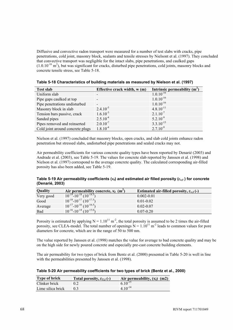
68 RIVM report 711701049
Diffusive and convective radon transport were measured for a number of test slabs with cracks, pipe penetrations, cold joint, masonry block, sealants and tensile stresses by Nielsont et al. (1997). They concluded that convective transport was negligible for the intact slabs, pipe penetrations, and caulked gaps (1.0.10-16 m2), but was significant for cracks, disturbed pipe penetrations, cold joints, masonry blocks and concrete tensile stress, see Table 5-18.
Table 5-18 Characteristics of building materials as measured by Nielson et al. (1997)
Test slab Effective crack width, w (m) Intrinsic permeability (m2) Uniform slab - 1.0.10-16 Pipe gaps caulked at top - 1.0.10-16 Pipe penetrations undisturbed - 1.0.10-16 Masonry block in slab 2.4.10-5 4.8.10-11 Tension bars passive, crack 1.6.10-3 2.1.10-7 Sanded pipes 2.5.10-4 5.2.10-9 Pipes removed and reinserted 2.0.10-7 3.3.10-15 Cold joint around concrete plugs 1.8.10-4 2.7.10-9 Nielson et al. (1997) concluded that masonry blocks, open cracks, and slab cold joints enhance radon penetration but stressed slabs, undisturbed pipe penetrations and sealed cracks may not. Air permeability coefficients for various concrete quality types have been reported by Denarié (2003) and Andrade et al. (2003), see Table 5-19. The values for concrete slab reported by Janssen et al. (1998) and Nielson et al. (1997) correspond to the average concrete quality. The calculated corresponding air-filled porosity has also been added, see Table 5-19.
Table 5-19 Air permeability coefficients (κf) and estimated air filled porosity (εv,f ) for concrete (Denarié, 2003)
Quality Air permeability concrete, κf (m2) Estimated air-filled porosity, εv,f (-) Very good 10-19-10-18 (10-18.5) 0.002-0.01 Good 10-18-10-17 (10-17.5) 0.01-0.02 Average 10-17-10-16 (10-16.5) 0.02-0.07 Bad 10-16-10-14 (10-15.0) 0.07-0.20 Porosity is estimated by applying N = 1.1011 m-2, the total porosity is assumed to be 2 times the air-filled porosity, see CLEA-model. The total number of openings N = 1.1011 m-2 leads to common values for pore diameters for concrete, which are in the range of 50 to 500 nm. The value reported by Janssen et al. (1998) matches the value for average to bad concrete quality and may be on the high side for newly poured concrete and especially pre-cast concrete building elements. The air permeability for two types of brick from Bentz et al. (2000) presented in Table 5-20 is well in line with the permeabilities presented by Janssen et al. (1998).
Table 5-20 Air permeability coefficients for two types of brick (Bentz et al., 2000)
Type of brick Total porosity, εT,f (-) Air permeability, (κf) (m2) Clinker brick 0.2 6.10-15 Lime silica brick 0.3 4.10-14
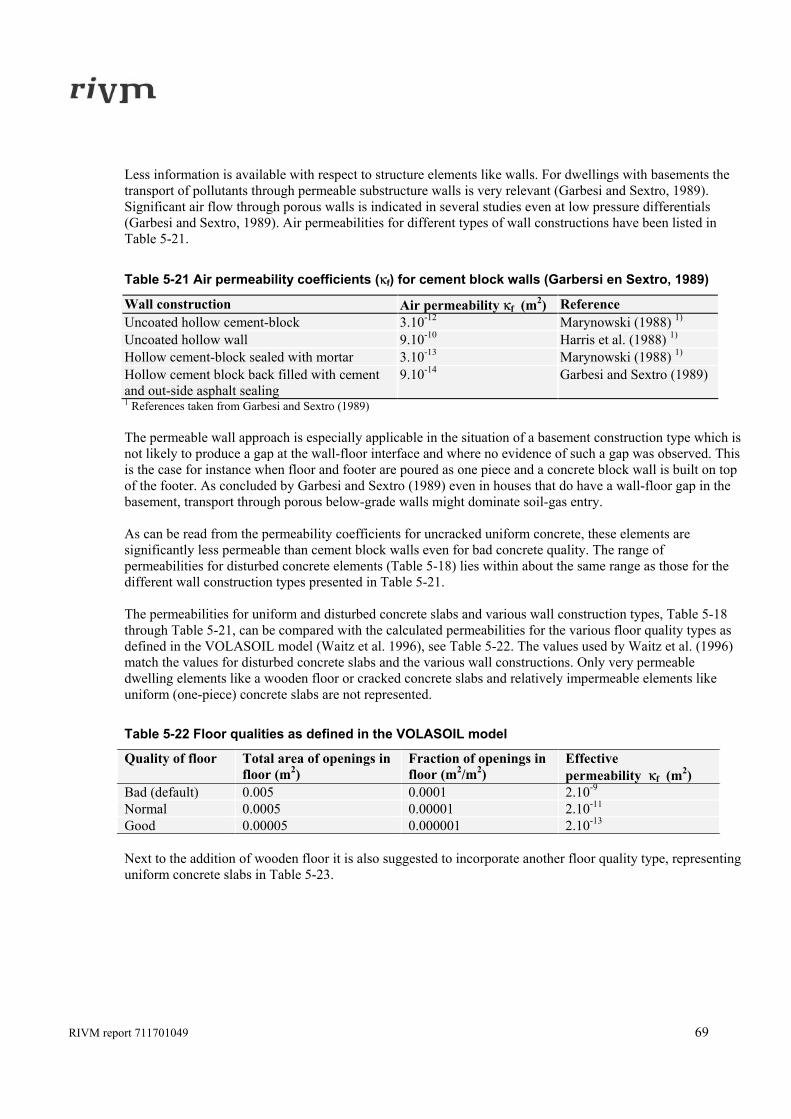
RIVM report 711701049 69
Less information is available with respect to structure elements like walls. For dwellings with basements the transport of pollutants through permeable substructure walls is very relevant (Garbesi and Sextro, 1989). Significant air flow through porous walls is indicated in several studies even at low pressure differentials (Garbesi and Sextro, 1989). Air permeabilities for different types of wall constructions have been listed in Table 5-21.
Table 5-21 Air permeability coefficients (κf) for cement block walls (Garbersi en Sextro, 1989)
Wall construction Air permeability κf (m2) Reference Uncoated hollow cement-block 3.10-12 Marynowski (1988) 1)
Uncoated hollow wall 9.10-10 Harris et al. (1988) 1)
Hollow cement-block sealed with mortar 3.10-13 Marynowski (1988) 1)
Hollow cement block back filled with cement and out-side asphalt sealing
9.10-14 Garbesi and Sextro (1989)
1 References taken from Garbesi and Sextro (1989) The permeable wall approach is especially applicable in the situation of a basement construction type which is not likely to produce a gap at the wall-floor interface and where no evidence of such a gap was observed. This is the case for instance when floor and footer are poured as one piece and a concrete block wall is built on top of the footer. As concluded by Garbesi and Sextro (1989) even in houses that do have a wall-floor gap in the basement, transport through porous below-grade walls might dominate soil-gas entry. As can be read from the permeability coefficients for uncracked uniform concrete, these elements are significantly less permeable than cement block walls even for bad concrete quality. The range of permeabilities for disturbed concrete elements (Table 5-18) lies within about the same range as those for the different wall construction types presented in Table 5-21. The permeabilities for uniform and disturbed concrete slabs and various wall construction types, Table 5-18 through Table 5-21, can be compared with the calculated permeabilities for the various floor quality types as defined in the VOLASOIL model (Waitz et al. 1996), see Table 5-22. The values used by Waitz et al. (1996) match the values for disturbed concrete slabs and the various wall constructions. Only very permeable dwelling elements like a wooden floor or cracked concrete slabs and relatively impermeable elements like uniform (one-piece) concrete slabs are not represented.
Table 5-22 Floor qualities as defined in the VOLASOIL model
Quality of floor Total area of openings in floor (m2)
Fraction of openings in floor (m2/m2)
Effective permeability κf (m2)
Bad (default) 0.005 0.0001 2.10-9
Normal 0.0005 0.00001 2.10-11 Good 0.00005 0.000001 2.10-13 Next to the addition of wooden floor it is also suggested to incorporate another floor quality type, representing uniform concrete slabs in Table 5-23.
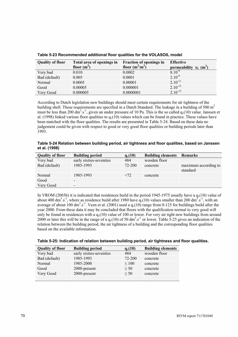
70 RIVM report 711701049
Table 5-23 Recommended additional floor qualities for the VOLASOIL model
Quality of floor Total area of openings in floor (m2)
Fraction of openings in floor (m2/m2)
Effective permeability κf (m2)
Very bad 0.010 0.0002 8.10-9 Bad (default) 0.005 0.0001 2.10-9
Normal 0.0005 0.00001 2.10-11 Good 0.00005 0.000001 2.10-13 Very Good 0.000005 0.0000001 2.10-15 According to Dutch legislation new buildings should meet certain requirements for air tightness of the building shell. These requirements are specified in a Dutch Standard. The leakage in a building of 500 m3 must be less than 200 dm3.s-1, given an under pressure of 10 Pa. This is the so called qv(10) value. Janssen et al. (1998) linked various floor qualities to qv(10) values which can be found in practice. These values have been matched with the floor qualities. The results are presented in Table 5-24. Based on these data no judgement could be given with respect to good or very good floor qualities or building periods later than 1993.
Table 5-24 Relation between building period, air tightness and floor qualities, based on Janssen et al. (1998)
Quality of floor Building period qv(10) Building elements Remarks Very bad early sixties-seventies 484 wooden floor Bad (default) 1985-1993 72-200 concrete maximum according to
standard Normal 1985-1993 <72 concrete Good - Very Good - In VROM (2003b) it is indicated that residences build in the period 1945-1975 usually have a qv(10) value of about 400 dm3.s-1, where as residence build after 1980 have qv(10) values smaller than 200 dm3.s-1, with an average of about 100 dm3.s-1. Veen et al. (2001) used a qv(10) range from 0-125 for buildings build after the year 2000. From these data it may be concluded that floors with the qualification normal to very good will only be found in residences with a qv(10) value of 100 or lower. For very air tight new buildings from around 2000 or later this will be in the range of a qv(10) of 50 dm3.s-1 or lower. Table 5-25 gives an indication of the relation between the building period, the air tightness of a building and the corresponding floor qualities based on the available information.
Table 5-25: Indication of relation between building period, air tightness and floor qualities.
Quality of floor Building period qv(10) Building elements Very bad early sixties-seventies 484 wooden floor Bad (default) 1985-1993 72-200 concrete Normal 1985-2000 ≤ 100 concrete Good 2000-present ≤ 50 concrete Very Good 2000-present ≤ 50 concrete
RIVM report 711701049 71
5.4.6 Perimeter seam gap and crack ratio The crack width and crack ratio are related. Assuming a square house and that the only crack is a continuous edge crack between the foundation slab and wall (‘perimeter crack’), the crack ratio and crack width are related as follows:
crack
Bcrack X
Ar μ= (Equation 5.1)
where μ ratio between crack area and enclosed space area below grade Acrack/AB [-] 0<μ<1, values for μ may range from 0.01 to 0.0001 rcrack radius of the crack or crack width [m] There is little information available on crack width or crack ratio. Some information on the crack ratio and crack width is reported by US-EPA (2003). The selected default crack width is 1 mm for the slab-on-grade scenario and 0.5 mm for the basement scenario (US-EPA, 2003). One approach used by radon researchers is to back calculate crack ratios using a model for soil gas flow through cracks and the results of measured soil gas flow rates into a building. For example, the back-calculated values for a slab/wall edge crack based on soil gas-entry rates reported by e.g. Nazaroff et al. (1985) range from approximately 0.0001 to 0.001. Another possible approach is to measure crack openings although this, in practice, is difficult to do. Crack widths range from hairline cracks up to 5 mm wide, while the total crack length per house ranged from 2.5 m to 17.3 m. Most crack widths were less than 1 mm. Mowris and Fisk (1988) estimated the shrinkage gap based on typical concrete shrinkage strains of 3 to 6.10-4 m.m-1. By assuming that the dimensions of concrete slabs range between 5 and 25 m, the floor-wall gaps that result from shrinkage would typically have a width of 0.001 and 0.015 m. The suggested defaults for crack ratio in regulatory guidance, literature and models also vary. In ASTM E1739-95, a default crack ratio of 0.01 is used. US-EPA, 2003 uses a crack ratio of 0.00038 for the slab-on-grade scenario and 0.0002 for the basement scenario. Using the default value for the crack width of 0.001 m and a foundation footprint area of 5 x 10 m = 50 m2, the crack ratio can be calculated for the building with a slab on grade floor and the building with a basement. The area of the enclosed space for the basement is based on the depth of the basement. For a dwelling with a slab on grade floor the depth of the floor below grade is assumed to be 0.15 m. From these parameters the default crack ratio is 0.00055 for a building with a slab on grade floor and 0.00027 for the basement scenario.
5.4.7 Ventilation characteristics, living room VOLASOIL uses the basic indoor ventilation flow (see Table 5-26) to calculate the ventilation of the indoor space. The ventilation rate of indoor space is an important parameter, because it contributes for a major part (10%) to the uncertainty of the model output (Waitz et al., 1996). The ventilation rate (1.h-1) is a better basis than the ventilation flow (m3.h-1), this because the ventilation rate is independent of the size of the building. The ventilation rate is calculated from the ventilation flow and a volume indoor space of 150 m3. In VOLASOIL the basic ventilation flow between 25 m3.h-1 (bad) and 150 m3.h-1 (very good) can be chosen. The normal rate of 75 m3.h-1 is the minimum according to the ‘bouwbesluit’ (NEN 1087). According to the ‘bouwbesluit 2003’ Art. 3.46 (Table 3.46.1), the minimum ventilation rate is 7 dm3.s-1, which is about 25 m3.h-1 per person (VROM, 2005). For three persons this results in a ventilation rate of 75 m3.h-1. The higher the ventilation rate, the lower the indoor air concentration.
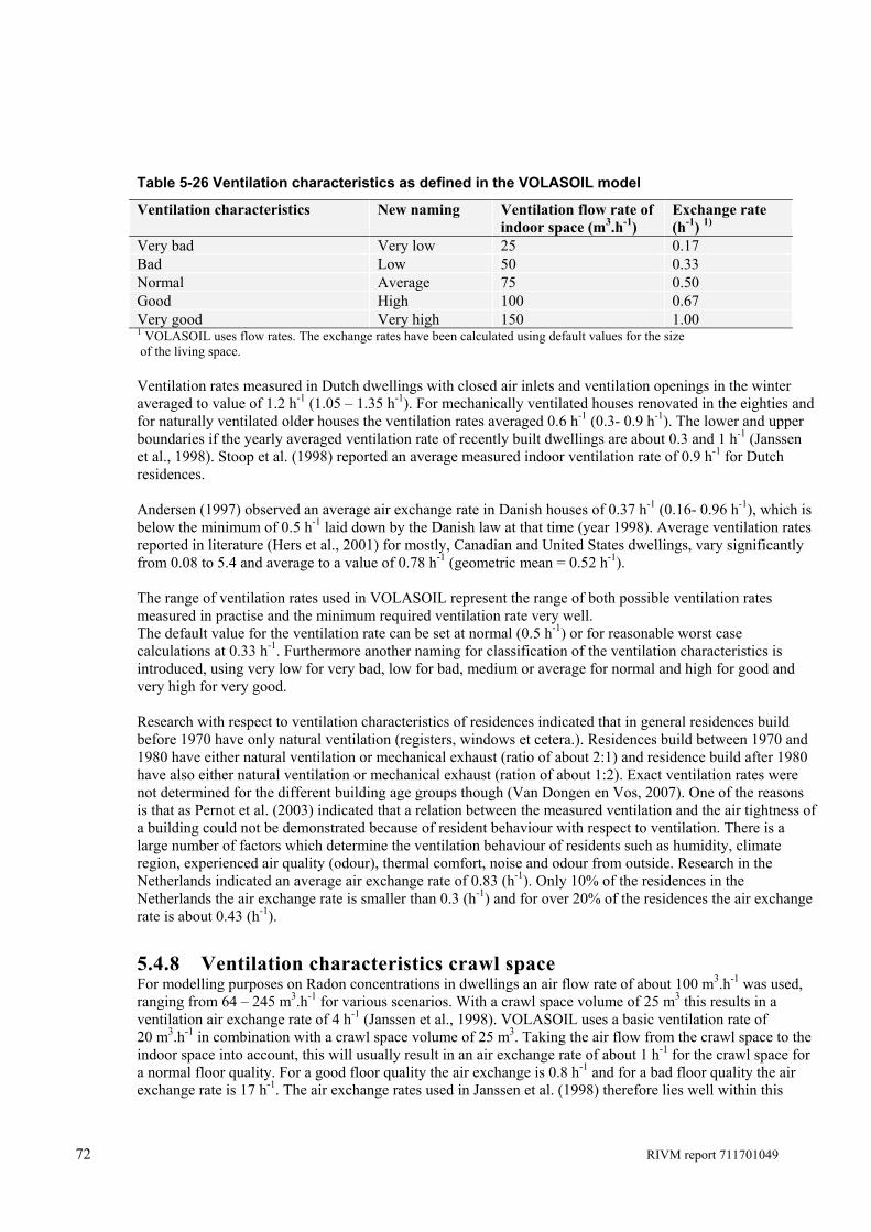
72 RIVM report 711701049
Table 5-26 Ventilation characteristics as defined in the VOLASOIL model
Ventilation characteristics New naming Ventilation flow rate of indoor space (m3.h-1)
Exchange rate (h-1) 1)
Very bad Very low 25 0.17 Bad Low 50 0.33 Normal Average 75 0.50 Good High 100 0.67 Very good Very high 150 1.00 1 VOLASOIL uses flow rates. The exchange rates have been calculated using default values for the size of the living space. Ventilation rates measured in Dutch dwellings with closed air inlets and ventilation openings in the winter averaged to value of 1.2 h-1 (1.05 – 1.35 h-1). For mechanically ventilated houses renovated in the eighties and for naturally ventilated older houses the ventilation rates averaged 0.6 h-1 (0.3- 0.9 h-1). The lower and upper boundaries if the yearly averaged ventilation rate of recently built dwellings are about 0.3 and 1 h-1 (Janssen et al., 1998). Stoop et al. (1998) reported an average measured indoor ventilation rate of 0.9 h-1 for Dutch residences. Andersen (1997) observed an average air exchange rate in Danish houses of 0.37 h-1 (0.16- 0.96 h-1), which is below the minimum of 0.5 h-1 laid down by the Danish law at that time (year 1998). Average ventilation rates reported in literature (Hers et al., 2001) for mostly, Canadian and United States dwellings, vary significantly from 0.08 to 5.4 and average to a value of 0.78 h-1 (geometric mean = 0.52 h-1). The range of ventilation rates used in VOLASOIL represent the range of both possible ventilation rates measured in practise and the minimum required ventilation rate very well. The default value for the ventilation rate can be set at normal (0.5 h-1) or for reasonable worst case calculations at 0.33 h-1. Furthermore another naming for classification of the ventilation characteristics is introduced, using very low for very bad, low for bad, medium or average for normal and high for good and very high for very good. Research with respect to ventilation characteristics of residences indicated that in general residences build before 1970 have only natural ventilation (registers, windows et cetera.). Residences build between 1970 and 1980 have either natural ventilation or mechanical exhaust (ratio of about 2:1) and residence build after 1980 have also either natural ventilation or mechanical exhaust (ration of about 1:2). Exact ventilation rates were not determined for the different building age groups though (Van Dongen en Vos, 2007). One of the reasons is that as Pernot et al. (2003) indicated that a relation between the measured ventilation and the air tightness of a building could not be demonstrated because of resident behaviour with respect to ventilation. There is a large number of factors which determine the ventilation behaviour of residents such as humidity, climate region, experienced air quality (odour), thermal comfort, noise and odour from outside. Research in the Netherlands indicated an average air exchange rate of 0.83 (h-1). Only 10% of the residences in the Netherlands the air exchange rate is smaller than 0.3 (h-1) and for over 20% of the residences the air exchange rate is about 0.43 (h-1).
5.4.8 Ventilation characteristics crawl space For modelling purposes on Radon concentrations in dwellings an air flow rate of about 100 m3.h-1 was used, ranging from 64 – 245 m3.h-1 for various scenarios. With a crawl space volume of 25 m3 this results in a ventilation air exchange rate of 4 h-1 (Janssen et al., 1998). VOLASOIL uses a basic ventilation rate of 20 m3.h-1 in combination with a crawl space volume of 25 m3. Taking the air flow from the crawl space to the indoor space into account, this will usually result in an air exchange rate of about 1 h-1 for the crawl space for a normal floor quality. For a good floor quality the air exchange is 0.8 h-1 and for a bad floor quality the air exchange rate is 17 h-1. The air exchange rates used in Janssen et al. (1998) therefore lies well within this
RIVM report 711701049 73
range. Fast et al. (1987) did extensive research on measurements of air-exchange rate of about hundred crawl spaces in the Netherlands at different locations. A geometrically weighted mean air-exchange rate of 1.0 h-1 can be derived from the data presented by Fast et al. (1987). The measured air-exchange rate lies in the range of 0.03 – 7.4 h-1. Stoop et al. (1998) reported an average measured ventilation rate of 1.1 h-1 for the crawl space in the Netherlands.
5.5 Generic input parameters In this section the parameters are defined that in general cannot or do not have to be changed. The specific parameters are listed in Table 5-27.
Table 5-27 Parameters that in general cannot or do not have to be changed
Parameter Unit Symbol Building Air pressure difference between soil and crawl space, crawl space and building, building with cellar and soil, building (slab on grade) and soil
Pa ΔPcs, ΔPic, ΔPis
Geometry (size) of the building/crawl space/cel Depth of crawl space, basement Floor area of building
m3
m m2
Vi,Vc and Vb dc, db Af
Floor/wall thickness crawl space slab on grade basement
m Lw, Lf
5.5.1 Air pressure difference For this parameter a distinction can be made between soil to crawl space and crawl space to indoor air pressure difference, see Figure 5-2. When no crawlspace is available only the air pressure difference between soil and indoor air (including basement) is accounted for. Air pressure differences can be caused by wind, temperature differences and barometric changes. A higher air pressure difference (higher house depressurisation) results in a higher indoor air flow from the soil, crawl space or basement. The air pressure difference between crawlspace and soil contributes largely (60%) to the uncertainty of the indoor air concentration (Waitz et al., 1996).
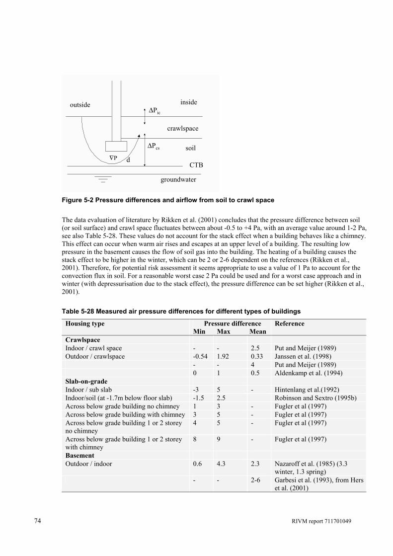
74 RIVM report 711701049
d
groundwater
soil
crawlspace
insideoutside
ΔPcs
ΔPic
CTB∇P
Figure 5-2 Pressure differences and airflow from soil to crawl space
The data evaluation of literature by Rikken et al. (2001) concludes that the pressure difference between soil (or soil surface) and crawl space fluctuates between about -0.5 to +4 Pa, with an average value around 1-2 Pa, see also Table 5-28. These values do not account for the stack effect when a building behaves like a chimney. This effect can occur when warm air rises and escapes at an upper level of a building. The resulting low pressure in the basement causes the flow of soil gas into the building. The heating of a building causes the stack effect to be higher in the winter, which can be 2 or 2-6 dependent on the references (Rikken et al., 2001). Therefore, for potential risk assessment it seems appropriate to use a value of 1 Pa to account for the convection flux in soil. For a reasonable worst case 2 Pa could be used and for a worst case approach and in winter (with depressurisation due to the stack effect), the pressure difference can be set higher (Rikken et al., 2001).
Table 5-28 Measured air pressure differences for different types of buildings
Housing type Pressure difference Min Max Mean
Reference
Crawlspace Indoor / crawl space - - 2.5 Put and Meijer (1989) Outdoor / crawlspace -0.54 1.92 0.33 Janssen et al. (1998) - - 4 Put and Meijer (1989) 0 1 0.5 Aldenkamp et al. (1994) Slab-on-grade Indoor / sub slab -3 5 - Hintenlang et al.(1992) Indoor/soil (at -1.7m below floor slab) -1.5 2.5 Robinson and Sextro (1995b) Across below grade building no chimney 1 3 - Fugler et al (1997) Across below grade building with chimney 3 5 - Fugler et al (1997) Across below grade building 1 or 2 storey no chimney
4 5 - Fugler et al (1997)
Across below grade building 1 or 2 storey with chimney
8 9 - Fugler et al (1997)
Basement Outdoor / indoor 0.6 4.3 2.3
Nazaroff et al. (1985) (3.3 winter, 1.3 spring)
- - 2-6 Garbesi et al. (1993), from Hers et al. (2001)
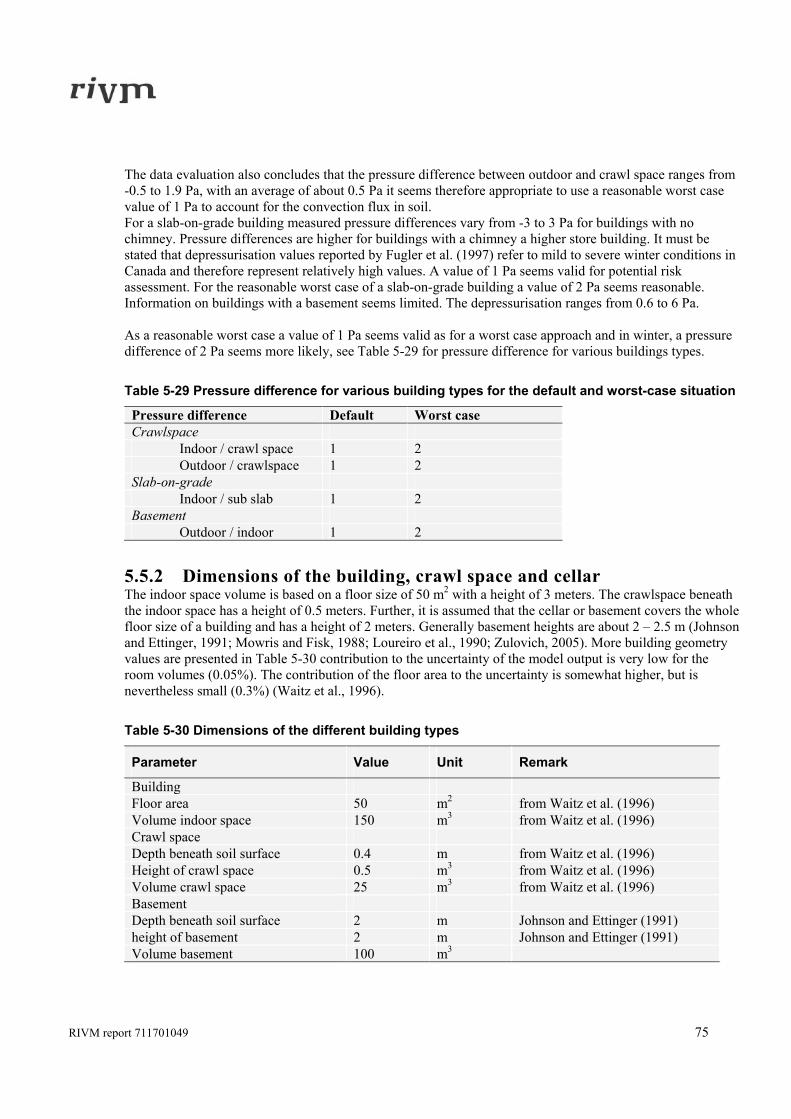
RIVM report 711701049 75
The data evaluation also concludes that the pressure difference between outdoor and crawl space ranges from -0.5 to 1.9 Pa, with an average of about 0.5 Pa it seems therefore appropriate to use a reasonable worst case value of 1 Pa to account for the convection flux in soil. For a slab-on-grade building measured pressure differences vary from -3 to 3 Pa for buildings with no chimney. Pressure differences are higher for buildings with a chimney a higher store building. It must be stated that depressurisation values reported by Fugler et al. (1997) refer to mild to severe winter conditions in Canada and therefore represent relatively high values. A value of 1 Pa seems valid for potential risk assessment. For the reasonable worst case of a slab-on-grade building a value of 2 Pa seems reasonable. Information on buildings with a basement seems limited. The depressurisation ranges from 0.6 to 6 Pa. As a reasonable worst case a value of 1 Pa seems valid as for a worst case approach and in winter, a pressure difference of 2 Pa seems more likely, see Table 5-29 for pressure difference for various buildings types.
Table 5-29 Pressure difference for various building types for the default and worst-case situation
Pressure difference Default Worst case Crawlspace Indoor / crawl space 1 2 Outdoor / crawlspace 1 2 Slab-on-grade Indoor / sub slab 1 2 Basement Outdoor / indoor 1 2
5.5.2 Dimensions of the building, crawl space and cellar The indoor space volume is based on a floor size of 50 m2 with a height of 3 meters. The crawlspace beneath the indoor space has a height of 0.5 meters. Further, it is assumed that the cellar or basement covers the whole floor size of a building and has a height of 2 meters. Generally basement heights are about 2 – 2.5 m (Johnson and Ettinger, 1991; Mowris and Fisk, 1988; Loureiro et al., 1990; Zulovich, 2005). More building geometry values are presented in Table 5-30 contribution to the uncertainty of the model output is very low for the room volumes (0.05%). The contribution of the floor area to the uncertainty is somewhat higher, but is nevertheless small (0.3%) (Waitz et al., 1996).
Table 5-30 Dimensions of the different building types
Parameter Value Unit Remark
Building Floor area 50 m2 from Waitz et al. (1996) Volume indoor space 150 m3 from Waitz et al. (1996) Crawl space Depth beneath soil surface 0.4 m from Waitz et al. (1996) Height of crawl space 0.5 m3 from Waitz et al. (1996) Volume crawl space 25 m3 from Waitz et al. (1996) Basement Depth beneath soil surface 2 m Johnson and Ettinger (1991) height of basement 2 m Johnson and Ettinger (1991) Volume basement 100 m3
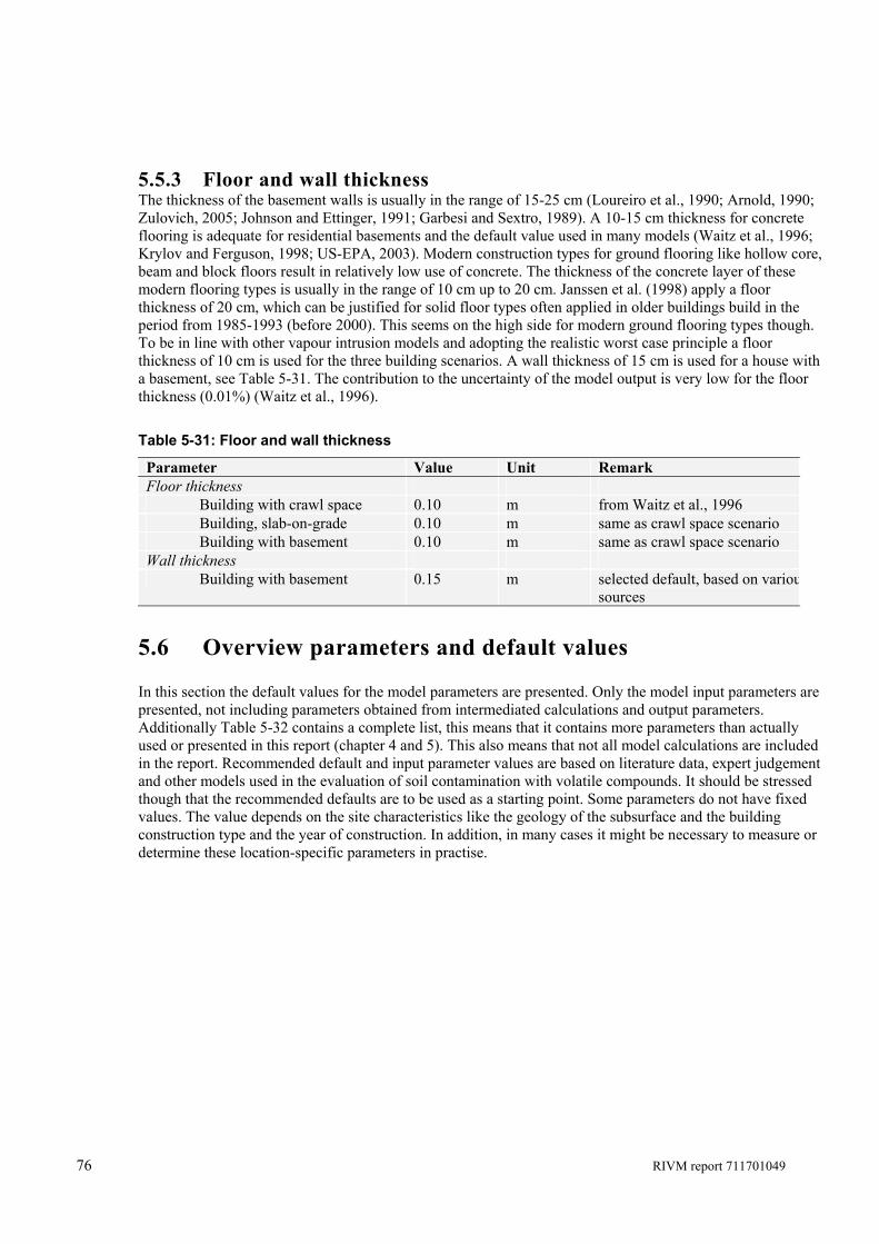
76 RIVM report 711701049
5.5.3 Floor and wall thickness The thickness of the basement walls is usually in the range of 15-25 cm (Loureiro et al., 1990; Arnold, 1990; Zulovich, 2005; Johnson and Ettinger, 1991; Garbesi and Sextro, 1989). A 10-15 cm thickness for concrete flooring is adequate for residential basements and the default value used in many models (Waitz et al., 1996; Krylov and Ferguson, 1998; US-EPA, 2003). Modern construction types for ground flooring like hollow core, beam and block floors result in relatively low use of concrete. The thickness of the concrete layer of these modern flooring types is usually in the range of 10 cm up to 20 cm. Janssen et al. (1998) apply a floor thickness of 20 cm, which can be justified for solid floor types often applied in older buildings build in the period from 1985-1993 (before 2000). This seems on the high side for modern ground flooring types though. To be in line with other vapour intrusion models and adopting the realistic worst case principle a floor thickness of 10 cm is used for the three building scenarios. A wall thickness of 15 cm is used for a house with a basement, see Table 5-31. The contribution to the uncertainty of the model output is very low for the floor thickness (0.01%) (Waitz et al., 1996).
Table 5-31: Floor and wall thickness
Parameter Value Unit Remark Floor thickness Building with crawl space 0.10 m from Waitz et al., 1996 Building, slab-on-grade 0.10 m same as crawl space scenario Building with basement 0.10 m same as crawl space scenario Wall thickness Building with basement 0.15 m selected default, based on variou
sources
5.6 Overview parameters and default values In this section the default values for the model parameters are presented. Only the model input parameters are presented, not including parameters obtained from intermediated calculations and output parameters. Additionally Table 5-32 contains a complete list, this means that it contains more parameters than actually used or presented in this report (chapter 4 and 5). This also means that not all model calculations are included in the report. Recommended default and input parameter values are based on literature data, expert judgement and other models used in the evaluation of soil contamination with volatile compounds. It should be stressed though that the recommended defaults are to be used as a starting point. Some parameters do not have fixed values. The value depends on the site characteristics like the geology of the subsurface and the building construction type and the year of construction. In addition, in many cases it might be necessary to measure or determine these location-specific parameters in practise.
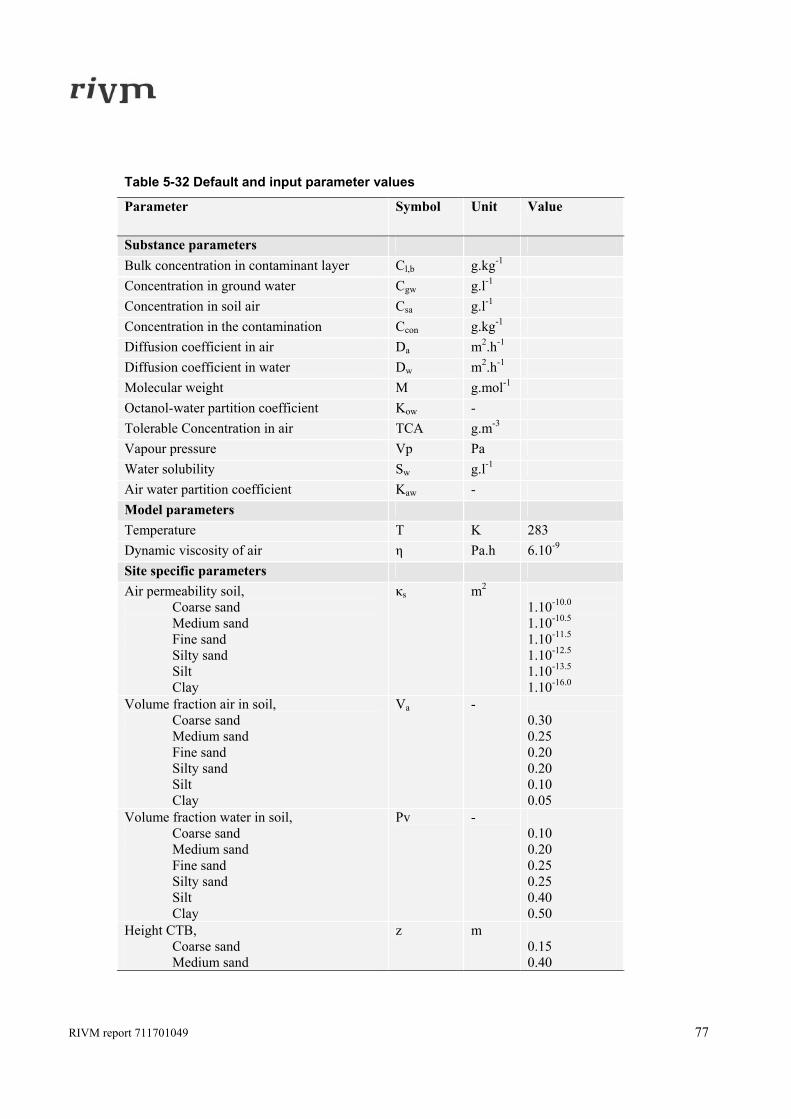
RIVM report 711701049 77
Table 5-32 Default and input parameter values
Parameter Symbol Unit Value
Substance parameters Bulk concentration in contaminant layer Cl,b g.kg-1 Concentration in ground water Cgw g.l-1 Concentration in soil air Csa g.l-1 Concentration in the contamination Ccon g.kg-1 Diffusion coefficient in air Da m2.h-1 Diffusion coefficient in water Dw m2.h-1 Molecular weight M g.mol-1 Octanol-water partition coefficient Kow - Tolerable Concentration in air TCA g.m-3 Vapour pressure Vp Pa Water solubility Sw g.l-1 Air water partition coefficient Kaw - Model parameters Temperature T K 283 Dynamic viscosity of air η Pa.h 6.10-9
Site specific parameters Air permeability soil, Coarse sand Medium sand Fine sand Silty sand Silt Clay
κs m2 1.10-10.0 1.10-10.5 1.10-11.5 1.10-12.5 1.10-13.5 1.10-16.0
Volume fraction air in soil, Coarse sand Medium sand Fine sand Silty sand Silt Clay
Va - 0.30 0.25 0.20 0.20 0.10 0.05
Volume fraction water in soil, Coarse sand Medium sand Fine sand Silty sand Silt Clay
Pv - 0.10 0.20 0.25 0.25 0.40 0.50
Height CTB, Coarse sand Medium sand
z m 0.15 0.40
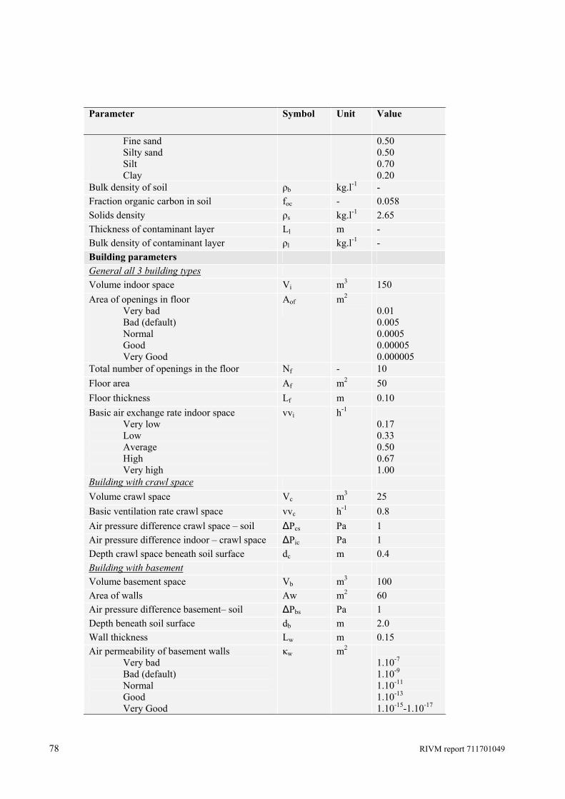
78 RIVM report 711701049
Parameter Symbol Unit Value
Fine sand Silty sand Silt Clay
0.50 0.50 0.70 0.20
Bulk density of soil ρb kg.l-1 - Fraction organic carbon in soil foc - 0.058 Solids density ρs kg.l-1 2.65 Thickness of contaminant layer Ll m - Bulk density of contaminant layer ρl kg.l-1 - Building parameters General all 3 building types Volume indoor space Vi m3 150 Area of openings in floor Very bad Bad (default) Normal Good Very Good
Aof
m2 0.01 0.005 0.0005 0.00005 0.000005
Total number of openings in the floor Nf - 10 Floor area Af m2 50 Floor thickness Lf m 0.10 Basic air exchange rate indoor space Very low Low Average High Very high
vvi h-1 0.17 0.33 0.50 0.67 1.00
Building with crawl space Volume crawl space Vc m3 25 Basic ventilation rate crawl space vvc h-1 0.8 Air pressure difference crawl space – soil ΔPcs Pa 1 Air pressure difference indoor – crawl space ΔPic Pa 1 Depth crawl space beneath soil surface dc m 0.4 Building with basement Volume basement space Vb m3 100 Area of walls Aw m2 60 Air pressure difference basement– soil ΔPbs Pa 1 Depth beneath soil surface db m 2.0 Wall thickness Lw m 0.15 Air permeability of basement walls Very bad Bad (default) Normal Good Very Good
κw m2 1.10-7 1.10-9 1.10-11 1.10-13 1.10-15-1.10-17
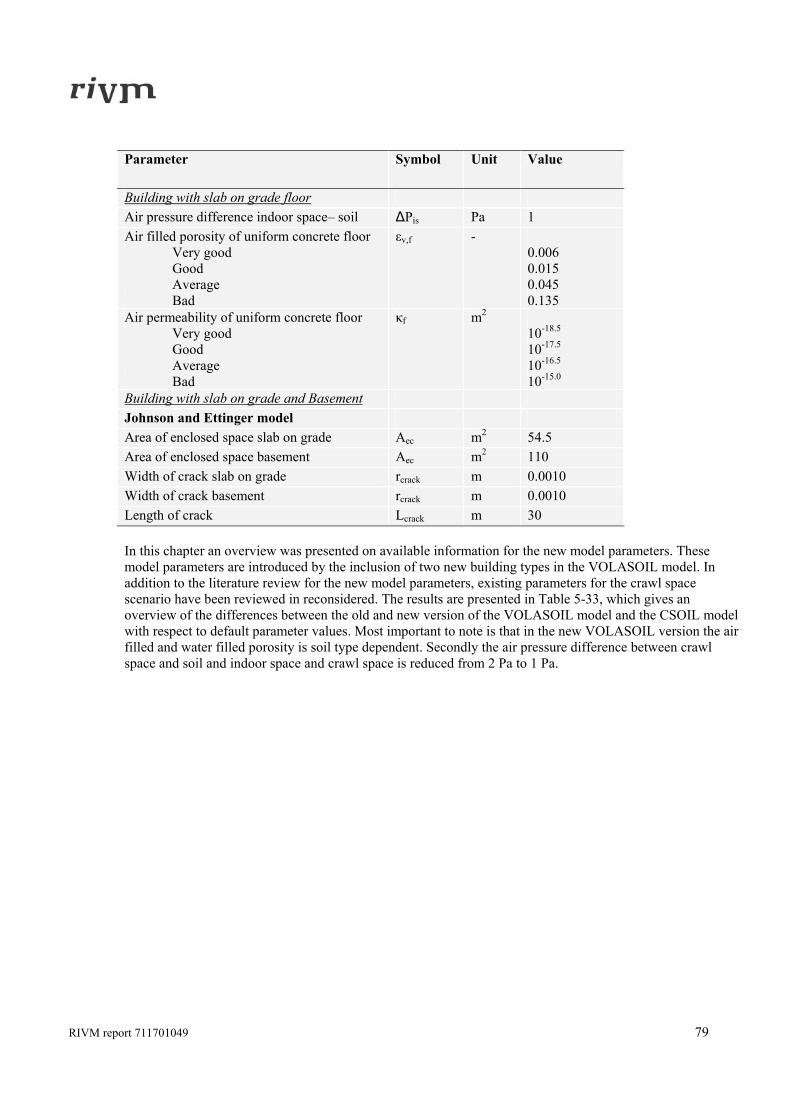
RIVM report 711701049 79
Parameter Symbol Unit Value
Building with slab on grade floor Air pressure difference indoor space– soil ΔPis Pa 1 Air filled porosity of uniform concrete floor Very good Good Average Bad
εv,f - 0.006 0.015 0.045 0.135
Air permeability of uniform concrete floor Very good Good Average Bad
κf m2 10-18.5 10-17.5 10-16.5 10-15.0
Building with slab on grade and Basement Johnson and Ettinger model Area of enclosed space slab on grade Aec m2 54.5 Area of enclosed space basement Aec m2 110 Width of crack slab on grade rcrack m 0.0010 Width of crack basement rcrack m 0.0010 Length of crack Lcrack m 30 In this chapter an overview was presented on available information for the new model parameters. These model parameters are introduced by the inclusion of two new building types in the VOLASOIL model. In addition to the literature review for the new model parameters, existing parameters for the crawl space scenario have been reviewed in reconsidered. The results are presented in Table 5-33, which gives an overview of the differences between the old and new version of the VOLASOIL model and the CSOIL model with respect to default parameter values. Most important to note is that in the new VOLASOIL version the air filled and water filled porosity is soil type dependent. Secondly the air pressure difference between crawl space and soil and indoor space and crawl space is reduced from 2 Pa to 1 Pa.
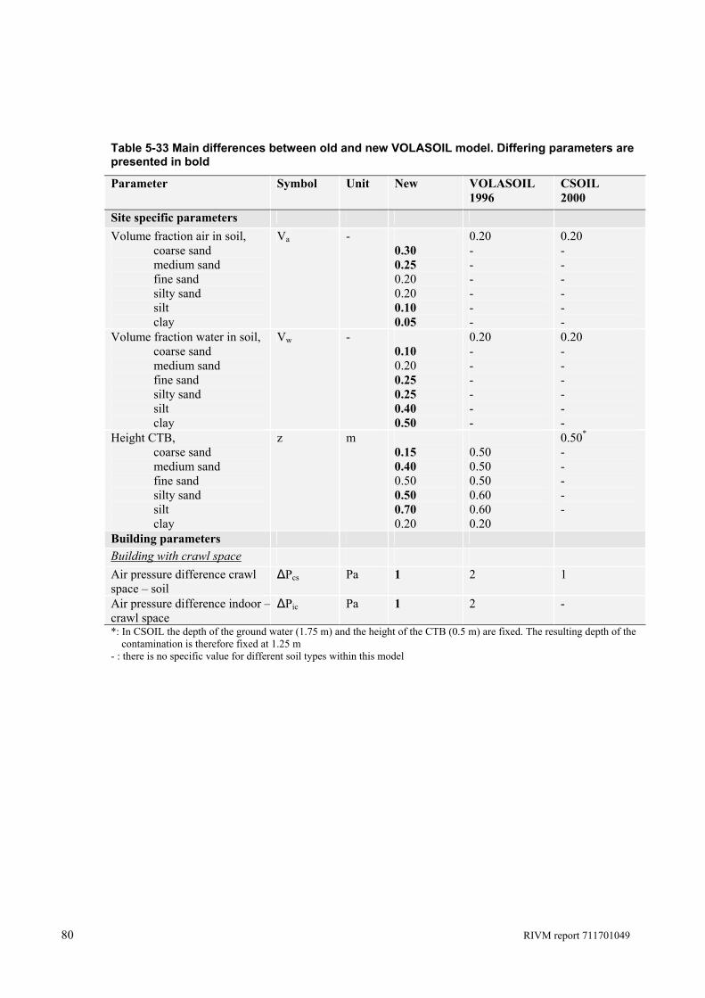
80 RIVM report 711701049
Table 5-33 Main differences between old and new VOLASOIL model. Differing parameters are presented in bold
Parameter Symbol Unit New VOLASOIL 1996
CSOIL 2000
Site specific parameters Volume fraction air in soil, coarse sand medium sand fine sand silty sand silt clay
Va - 0.30 0.25 0.20 0.20 0.10 0.05
0.20 - - - - - -
0.20 - - - - - -
Volume fraction water in soil, coarse sand medium sand fine sand silty sand silt clay
Vw - 0.10 0.20 0.25 0.25 0.40 0.50
0.20 - - - - - -
0.20 - - - - - -
Height CTB, coarse sand medium sand fine sand silty sand silt clay
z m 0.15 0.40 0.50 0.50 0.70 0.20
0.50 0.50 0.50 0.60 0.60 0.20
0.50*
- - - - -
Building parameters Building with crawl space Air pressure difference crawl space – soil
ΔPcs Pa 1 2 1
Air pressure difference indoor –crawl space
ΔPic Pa 1 2 -
*: In CSOIL the depth of the ground water (1.75 m) and the height of the CTB (0.5 m) are fixed. The resulting depth of the contamination is therefore fixed at 1.25 m - : there is no specific value for different soil types within this model
RIVM report 711701049 81
6. Uncertainty and sensitivity analysis
6.1 Introduction To get more insight in the model calculations for the standard building and the added building types, an uncertainty and sensitivity analysis was carried out. The analysis should indicate the most important model parameters and the uncertainty analysis should provide an indication of the uncertainty in the model output based on the uncertainties in the model (input) parameters. Additionally the analysis helps to understand the behaviour of the model and its calculations, and provide insight in the differences between the several model concepts and building types. The methodology of the sensitivity and uncertainty analysis is described in section 6.2. and the results are presented in section 6.3. Conclusions drawn from the sensitivity and uncertainty analysis are given in section 6.4.
6.2 Methods 6.2.1 Scenario analysis For the three building types, crawl space, slab on grade and basement, the indoor-air concentrations were taken as model output. Two soil types were differentiated, a sandy soil and a clayey (silt) soil because it is expected that the sensitivity of the model will largely depend on the soil type. Furthermore two different modelling concepts were analysed, the VOLASOIL model approach (laminar flow through a capillary) and the model approach described by Johnson and Ettinger (1991), the perimeter seam gap model. This was done in order to get insight in the behaviour and differences of these model concepts. Realistic default values were used for the input-parameters of these models based on the literature data in chapter 5 (see Table 6-2 and Appendix 9). For the uncertainty analysis, instead of a single value a range (or distribution) of values was used as input using the same data is a basis. The scenarios, which were taken into account in the sensitivity and uncertainty analysis, are summarised in Table 6-1:
Table 6-1 Scenarios for the uncertainty and sensitivity analysis
Model Crawlspace Slab-on-grade Basement VOLASOIL (capillary) X X X J & E(perimeter seam gap) X X These scenarios were calculated using two comparable substances: benzene and tetrachloroethylene (perchloroethylene or PER), and as stated before two soil types: silt and sandy soil.
6.2.2 Generic approach 6.2.2.1 Sensitivity analysis At first a sensitivity analysis was done for the two model approaches and the three building types, in order to indicate the degree of sensitivity of the output e.g. indoor air concentrations to variability in the input parameters. It shows the sensitivity to the model parameters independent of the actual uncertainty or variability. All parameters that are described in Table 6-2 are varied one at a time by ± 10 % around the mean. A uniform distribution is used for all parameters. A Monte Carlo sampling method is used with 200 runs, using the Crystal Ball add-in of Excel. The output indoor air concentrations are correlated to each parameter and a Normalized Regression Coefficient (NRC) is calculated:
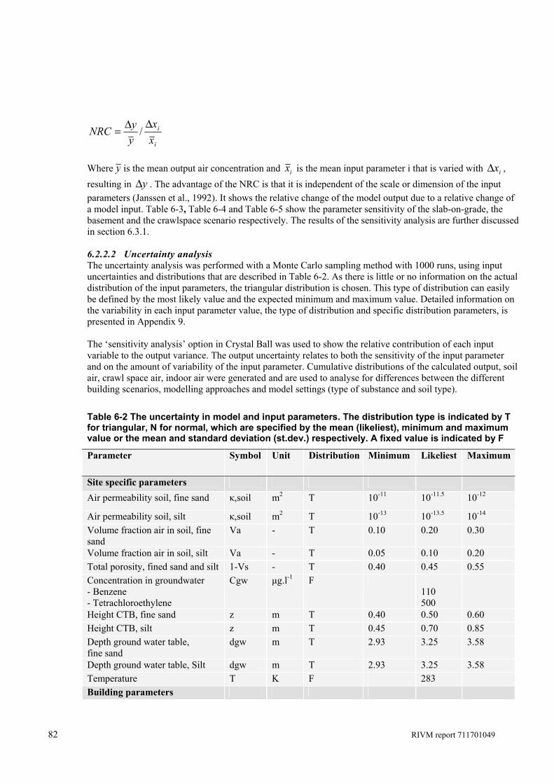
82 RIVM report 711701049
i
i
xx
yyNRC
ΔΔ= /
Where y is the mean output air concentration and ix is the mean input parameter i that is varied with ixΔ , resulting in yΔ . The advantage of the NRC is that it is independent of the scale or dimension of the input parameters (Janssen et al., 1992). It shows the relative change of the model output due to a relative change of a model input. Table 6-3, Table 6-4 and Table 6-5 show the parameter sensitivity of the slab-on-grade, the basement and the crawlspace scenario respectively. The results of the sensitivity analysis are further discussed in section 6.3.1. 6.2.2.2 Uncertainty analysis The uncertainty analysis was performed with a Monte Carlo sampling method with 1000 runs, using input uncertainties and distributions that are described in Table 6-2. As there is little or no information on the actual distribution of the input parameters, the triangular distribution is chosen. This type of distribution can easily be defined by the most likely value and the expected minimum and maximum value. Detailed information on the variability in each input parameter value, the type of distribution and specific distribution parameters, is presented in Appendix 9. The ‘sensitivity analysis’ option in Crystal Ball was used to show the relative contribution of each input variable to the output variance. The output uncertainty relates to both the sensitivity of the input parameter and on the amount of variability of the input parameter. Cumulative distributions of the calculated output, soil air, crawl space air, indoor air were generated and are used to analyse for differences between the different building scenarios, modelling approaches and model settings (type of substance and soil type).
Table 6-2 The uncertainty in model and input parameters. The distribution type is indicated by T for triangular, N for normal, which are specified by the mean (likeliest), minimum and maximum value or the mean and standard deviation (st.dev.) respectively. A fixed value is indicated by F
Parameter Symbol Unit Distribution Minimum Likeliest Maximum
Site specific parameters Air permeability soil, fine sand κ,soil m2 T 10-11 10-11.5 10-12
Air permeability soil, silt κ,soil m2 T 10-13 10-13.5 10-14 Volume fraction air in soil, fine sand
Va - T 0.10 0.20 0.30
Volume fraction air in soil, silt Va - T 0.05 0.10 0.20 Total porosity, fined sand and silt 1-Vs - T 0.40 0.45 0.55 Concentration in groundwater - Benzene - Tetrachloroethylene
Cgw μg.l-1 F 110 500
Height CTB, fine sand z m T 0.40 0.50 0.60 Height CTB, silt z m T 0.45 0.70 0.85 Depth ground water table, fine sand
dgw m T 2.93 3.25 3.58
Depth ground water table, Silt dgw m T 2.93 3.25 3.58 Temperature T K F 283 Building parameters
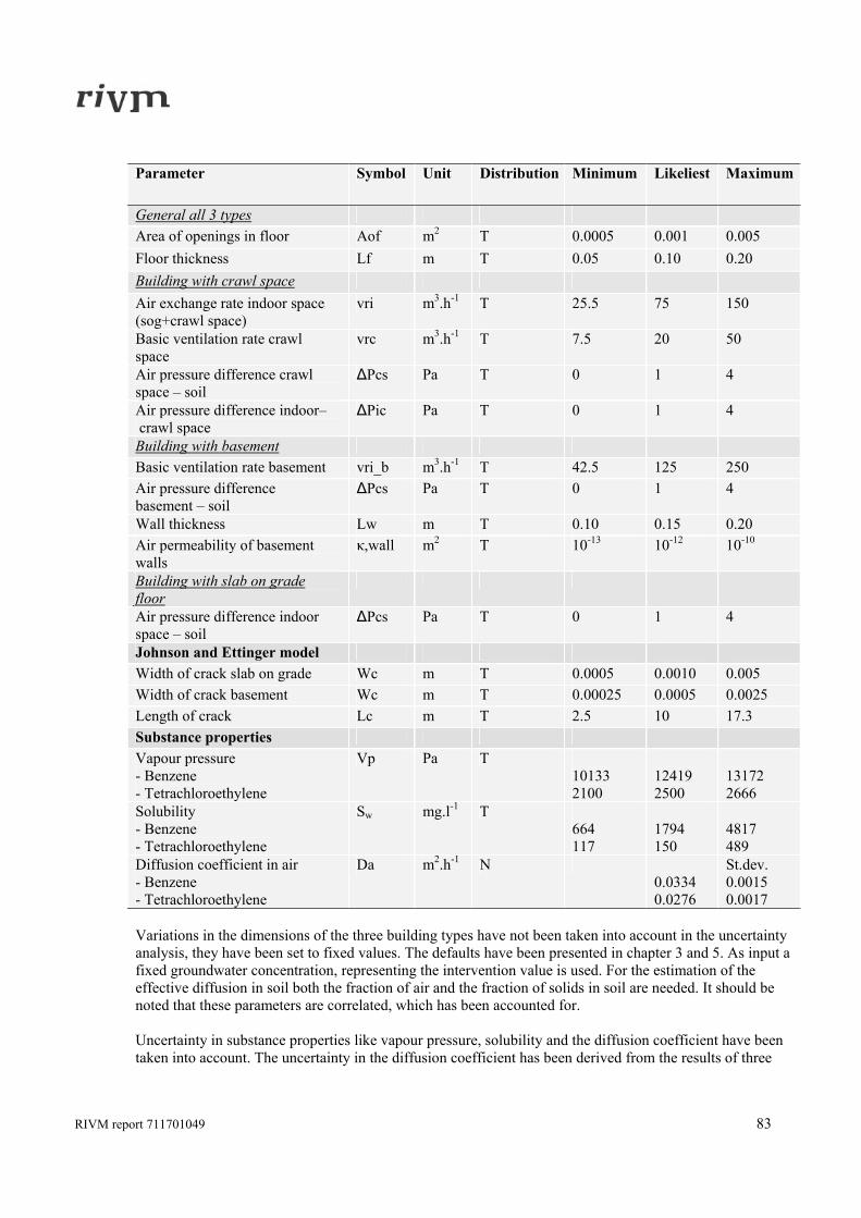
RIVM report 711701049 83
Parameter Symbol Unit Distribution Minimum Likeliest Maximum
General all 3 types Area of openings in floor Aof m2 T 0.0005 0.001 0.005 Floor thickness Lf m T 0.05 0.10 0.20 Building with crawl space Air exchange rate indoor space (sog+crawl space)
vri m3.h-1 T 25.5 75 150
Basic ventilation rate crawl space
vrc m3.h-1 T 7.5 20 50
Air pressure difference crawl space – soil
ΔPcs Pa T 0 1 4
Air pressure difference indoor– crawl space
ΔPic Pa T 0 1 4
Building with basement Basic ventilation rate basement vri_b m3.h-1 T 42.5 125 250 Air pressure difference basement – soil
ΔPcs Pa T 0 1 4
Wall thickness Lw m T 0.10 0.15 0.20 Air permeability of basement walls
κ,wall m2 T 10-13 10-12 10-10
Building with slab on grade floor
Air pressure difference indoor space – soil
ΔPcs Pa T 0 1 4
Johnson and Ettinger model Width of crack slab on grade Wc m T 0.0005 0.0010 0.005 Width of crack basement Wc m T 0.00025 0.0005 0.0025 Length of crack Lc m T 2.5 10 17.3 Substance properties Vapour pressure - Benzene - Tetrachloroethylene
Vp Pa T 10133 2100
12419 2500
13172 2666
Solubility - Benzene - Tetrachloroethylene
Sw mg.l-1 T 664 117
1794 150
4817 489
Diffusion coefficient in air - Benzene - Tetrachloroethylene
Da m2.h-1 N 0.0334 0.0276
St.dev. 0.0015 0.0017
Variations in the dimensions of the three building types have not been taken into account in the uncertainty analysis, they have been set to fixed values. The defaults have been presented in chapter 3 and 5. As input a fixed groundwater concentration, representing the intervention value is used. For the estimation of the effective diffusion in soil both the fraction of air and the fraction of solids in soil are needed. It should be noted that these parameters are correlated, which has been accounted for. Uncertainty in substance properties like vapour pressure, solubility and the diffusion coefficient have been taken into account. The uncertainty in the diffusion coefficient has been derived from the results of three
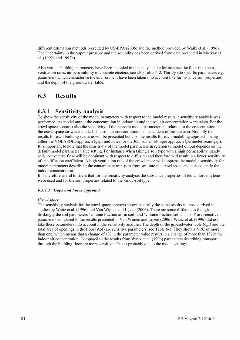
84 RIVM report 711701049
different estimation methods presented by US-EPA (2006) and the method provided by Waitz et al. (1996). The uncertainty in the vapour pressure and the solubility has been derived from data presented in Mackay et al. (1992a and 1992b). Also various building parameters have been included in the analysis like for instance the floor thickness, ventilation rates, air permeability of concrete etcetera, see also Table 6-2. Thirdly site specific parameters e.g. parameters which characterise the environment have been taken into account like for instance soil properties and the depth of the groundwater table.
6.3 Results
6.3.1 Sensitivity analysis To show the sensitivity of the model parameters with respect to the model results, a sensitivity analysis was performed. As model output the concentration in indoor air and the soil air concentration were taken. For the crawl space scenario also the sensitivity of the relevant model parameters in relation to the concentration in the crawl space air was included. The soil air concentration is independent of the scenario. Not only the results for each building scenario will be presented but also the results for each modelling approach, being either the VOLASOIL-approach (gaps and holes) or the Johnson en Ettinger approach (perimeter seam gap). It is important to note that the sensitivity of the model parameters in relation to model output depends on the default model parameter value setting. For instance when taking a soil type with a high permeability (sandy soil), convective flow will be dominant with respect to diffusion and therefore will result in a lower sensitivity of the diffusion coefficient. A high ventilation rate of the crawl space will suppress the model’s sensitivity for model parameters describing the contaminant transport from soil into the crawl space and consequently the indoor concentration. It is therefore useful to stress that for the sensitivity analysis the substance properties of tetrachloroethylene were used and for the soil properties related to the sandy-soil type. 6.3.1.1 Gaps and holes approach Crawl space The sensitivity analysis for the crawl space scenario shows basically the same results as those derived in studies by Waitz et al. (1996) and Van Wijnen and Lijzen (2006). There are some differences though. Strikingly the soil parameters ‘volume fraction air in soil’ and ‘volume fraction solids in soil’ are sensitive parameters compared to the results presented in Van Wijnen and Lijzen (2006). Waitz et al. (1996) did not take these parameters into account in the sensitivity analysis. The depth of the groundwater table (dgw) and the total area of openings in the floor (Aof) are sensitive parameters, see Table 6-3. They show a NRC of more than one, which means that a change of 1% in the parameter value results in a change of more than 1% in the indoor air concentration. Compared to the results from Waitz et al. (1996) parameters describing transport through the building floor are more sensitive. This is probably due to the model settings.
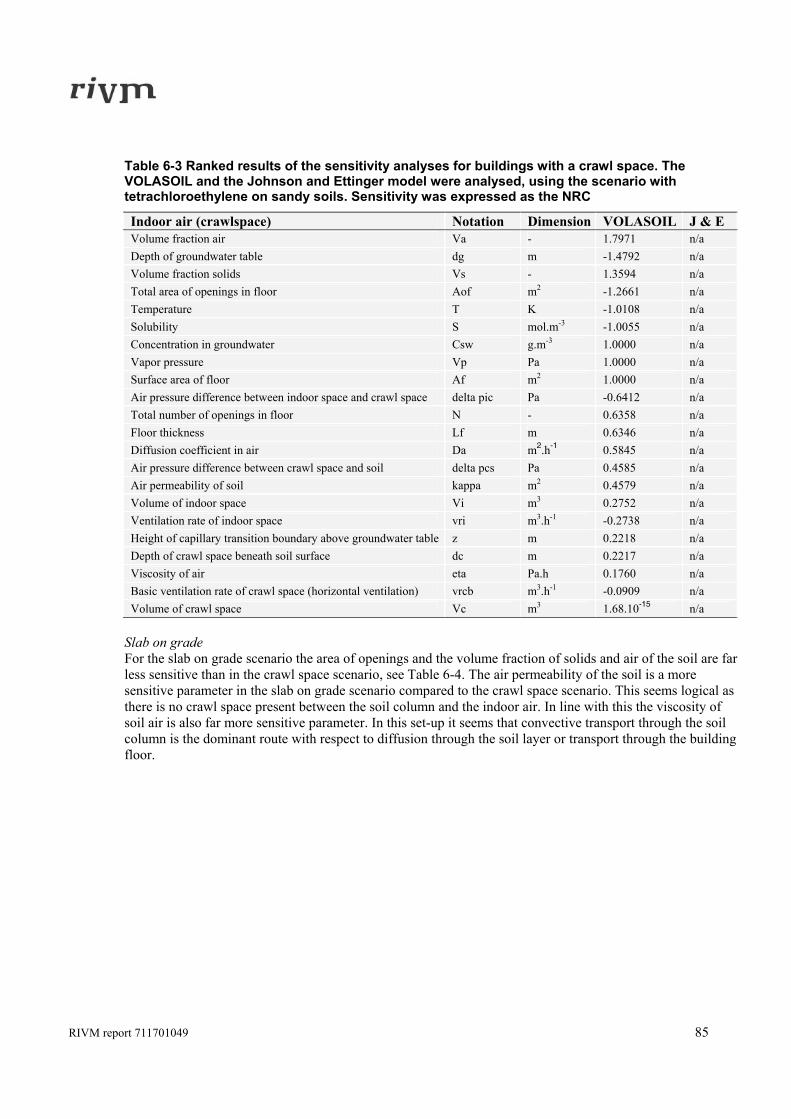
RIVM report 711701049 85
Table 6-3 Ranked results of the sensitivity analyses for buildings with a crawl space. The VOLASOIL and the Johnson and Ettinger model were analysed, using the scenario with tetrachloroethylene on sandy soils. Sensitivity was expressed as the NRC
Indoor air (crawlspace) Notation Dimension VOLASOIL J & E Volume fraction air Va - 1.7971 n/a Depth of groundwater table dg m -1.4792 n/a Volume fraction solids Vs - 1.3594 n/a Total area of openings in floor Aof m2 -1.2661 n/a Temperature T K -1.0108 n/a Solubility S mol.m-3 -1.0055 n/a Concentration in groundwater Csw g.m-3 1.0000 n/a Vapor pressure Vp Pa 1.0000 n/a Surface area of floor Af m2 1.0000 n/a Air pressure difference between indoor space and crawl space delta pic Pa -0.6412 n/a Total number of openings in floor N - 0.6358 n/a Floor thickness Lf m 0.6346 n/a Diffusion coefficient in air Da m2.h-1 0.5845 n/a Air pressure difference between crawl space and soil delta pcs Pa 0.4585 n/a Air permeability of soil kappa m2 0.4579 n/a Volume of indoor space Vi m3 0.2752 n/a Ventilation rate of indoor space vri m3.h-1 -0.2738 n/a Height of capillary transition boundary above groundwater table z m 0.2218 n/a Depth of crawl space beneath soil surface dc m 0.2217 n/a Viscosity of air eta Pa.h 0.1760 n/a Basic ventilation rate of crawl space (horizontal ventilation) vrcb m3.h-1 -0.0909 n/a Volume of crawl space Vc m3 1.68.10-15 n/a
Slab on grade For the slab on grade scenario the area of openings and the volume fraction of solids and air of the soil are far less sensitive than in the crawl space scenario, see Table 6-4. The air permeability of the soil is a more sensitive parameter in the slab on grade scenario compared to the crawl space scenario. This seems logical as there is no crawl space present between the soil column and the indoor air. In line with this the viscosity of soil air is also far more sensitive parameter. In this set-up it seems that convective transport through the soil column is the dominant route with respect to diffusion through the soil layer or transport through the building floor.
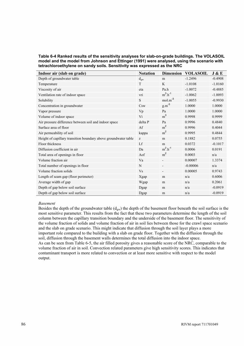
86 RIVM report 711701049
Table 6-4 Ranked results of the sensitivity analyses for slab-on-grade buildings. The VOLASOIL model and the model from Johnson and Ettinger (1991) were analysed, using the scenario with tetrachloroethylene on sandy soils. Sensitivity was expressed as the NRC
Indoor air (slab on grade) Notation Dimension VOLASOIL J & E Depth of groundwater table dgw m -1.2496 -0.4908 Temperature T K -1.0108 -1.0160 Viscosity of air eta Pa.h -1.0072 -0.4885 Ventilation rate of indoor space vri m3.h-1 -1.0062 -1.0093 Solubility S mol.m-3 -1.0055 -0.9930 Concentration in groundwater Csw g.m-3 1.0000 1.0000 Vapor pressure Vp Pa 1.0000 1.0000 Volume of indoor space Vi m3 0.9998 0.9999 Air pressure difference between soil and indoor space delta P Pa 0.9996 0.4840 Surface area of floor Af m2 0.9996 0.4044 Air permeability of soil kappa m2 0.9995 0.4844 Height of capillary transition boundary above groundwater table z m 0.1882 0.0755 Floor thickness Lf m 0.0372 -0.1017 Diffusion coefficient in air Da m2.h-1 0.0006 0.0191 Total area of openings in floor Aof m2 0.0003 n/a Volume fraction air Va - 0.00007 1.3374 Total number of openings in floor N - -0.00006 n/a Volume fraction solids Vs - 0.00005 0.9743 Length of seam gap (floor perimeter) Xgap m n/a 0.6006 Average width of gap Wgap m n/a 0.2061 Depth of gap below soil surface Dgap m n/a -0.0919 Depth of gap below soil surface Dgap m n/a -0.0919 Basement Besides the depth of the groundwater table (dgw) the depth of the basement floor beneath the soil surface is the most sensitive parameter. This results from the fact that these two parameters determine the length of the soil column between the capillary transition boundary and the underside of the basement floor. The sensitivity of the volume fraction of solids and volume fraction of air in soil lies between those for the crawl space scenario and the slab on grade scenario. This might indicate that diffusion through the soil layer plays a more important role compared to the building with a slab on grade floor. Together with the diffusion through the soil, diffusion through the basement walls determines the total diffusion into the indoor space. As can be seen from Table 6-5, the air filled porosity gives a reasonable score of the NRC, comparable to the volume fraction of air in soil. Convection related parameters give high sensitivity scores. This indicates that contaminant transport is more related to convection or at least more sensitive with respect to the model output.
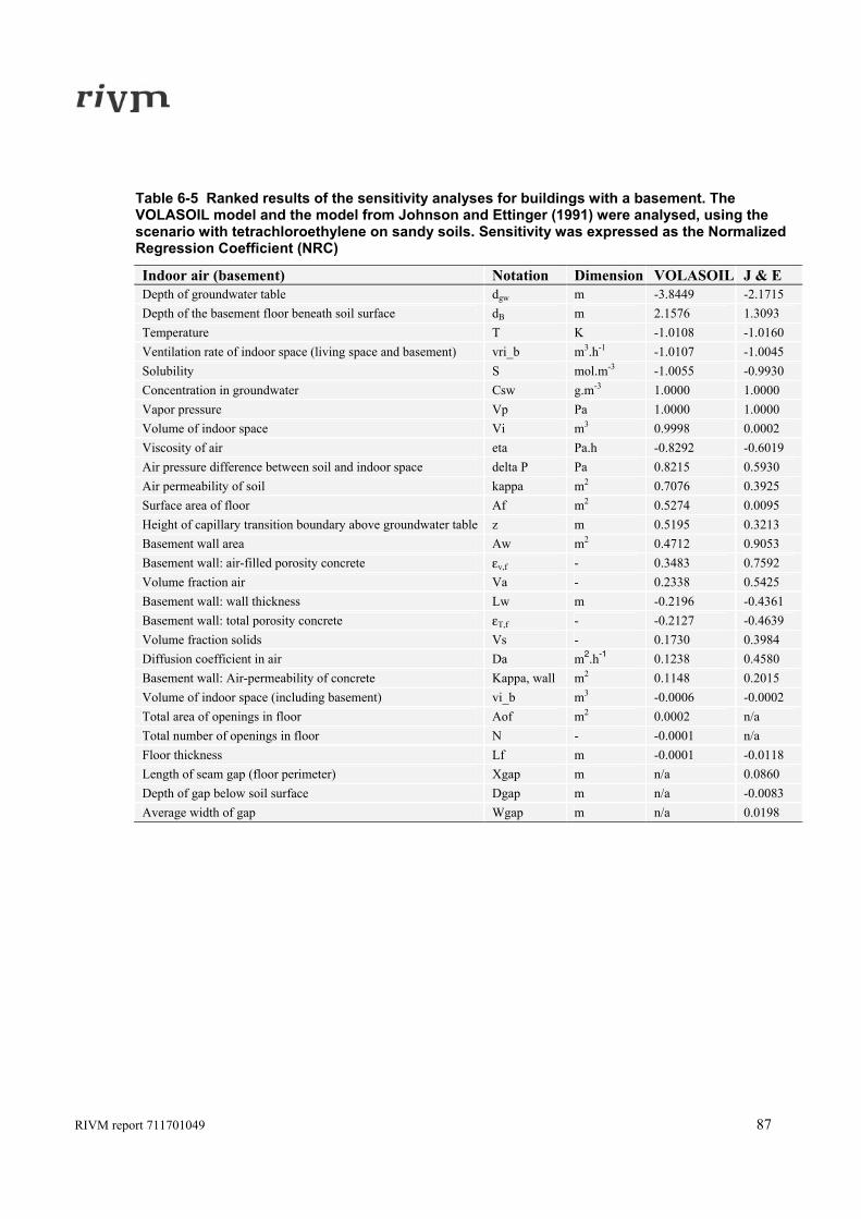
RIVM report 711701049 87
Table 6-5 Ranked results of the sensitivity analyses for buildings with a basement. The VOLASOIL model and the model from Johnson and Ettinger (1991) were analysed, using the scenario with tetrachloroethylene on sandy soils. Sensitivity was expressed as the Normalized Regression Coefficient (NRC)
Indoor air (basement) Notation Dimension VOLASOIL J & E Depth of groundwater table dgw m -3.8449 -2.1715 Depth of the basement floor beneath soil surface dB m 2.1576 1.3093 Temperature T K -1.0108 -1.0160 Ventilation rate of indoor space (living space and basement) vri_b m3.h-1 -1.0107 -1.0045 Solubility S mol.m-3 -1.0055 -0.9930 Concentration in groundwater Csw g.m-3 1.0000 1.0000 Vapor pressure Vp Pa 1.0000 1.0000 Volume of indoor space Vi m3 0.9998 0.0002 Viscosity of air eta Pa.h -0.8292 -0.6019 Air pressure difference between soil and indoor space delta P Pa 0.8215 0.5930 Air permeability of soil kappa m2 0.7076 0.3925 Surface area of floor Af m2 0.5274 0.0095 Height of capillary transition boundary above groundwater table z m 0.5195 0.3213 Basement wall area Aw m2 0.4712 0.9053 Basement wall: air-filled porosity concrete εv,f - 0.3483 0.7592 Volume fraction air Va - 0.2338 0.5425 Basement wall: wall thickness Lw m -0.2196 -0.4361 Basement wall: total porosity concrete εT,f - -0.2127 -0.4639 Volume fraction solids Vs - 0.1730 0.3984 Diffusion coefficient in air Da m2.h-1 0.1238 0.4580 Basement wall: Air-permeability of concrete Kappa, wall m2 0.1148 0.2015 Volume of indoor space (including basement) vi_b m3 -0.0006 -0.0002 Total area of openings in floor Aof m2 0.0002 n/a Total number of openings in floor N - -0.0001 n/a Floor thickness Lf m -0.0001 -0.0118 Length of seam gap (floor perimeter) Xgap m n/a 0.0860 Depth of gap below soil surface Dgap m n/a -0.0083 Average width of gap Wgap m n/a 0.0198
88 RIVM report 711701049
6.3.1.2 Johnson and Ettinger approach Slab on grade For the Johnson and Ettinger approach the results of the sensitivity analysis are comparable to the results for the gaps and holes approach. About the same parameters give the highest score of sensitivity, with a NRC of about one (Table 6-4). Only the depth of the groundwater table and the height of the capillary transition boundary are far less sensitive with respect to the model output. This comes from the fact that the flow rate of soil gas into the building is calculated differently by the Johnson en Ettinger approach. In the Johnson and Ettinger approach transport by convection through the soil layer is not considered, only transport by diffusion is accounted for. For the building floor both diffusion and convection are considered though. Therefore diffusion related parameters like the volume fraction of air in soil are more sensitive with respect to the model output. On the other hand convection related parameters like the air pressure difference are less sensitive compared to the VOLASOIL approach. The length of the perimeter seam gap seems to be the most sensitive parameter in the estimation of the flow rate of soil gas into the building. The average width of the gap, which is a difficult parameter to determine in practise, is less sensitive. Basement As for the gaps and holes approach, the depth of the groundwater table and the depth of the basement floor are the most sensitive parameters, see Table 6-5. Contrary to the slab on grade scenario, the model output is less sensitive to the specific parameters needed to estimate the flow rate of soil gas into the building. Compared to the slab-on grade scenario typical diffusion related parameters are more sensitive and convection related parameters are less sensitive compared to the slab on grade scenario. Also the surface area of the floor is a less sensitive parameter. This can be explained by the fact that for the basement, transport through the basement walls is also taken into account and fact that the transport through the basement walls is calculated comparable to the VOLASOIL approach. General The depth of the groundwater table is in almost all scenarios the most sensitive parameter, which means it should be estimated as accurate as possible in order increase the reliability of the model output. Other parameters with high model sensitivity are the vapour pressure and the solubility of the substance, the groundwater concentration, the pressure difference, the floor area and the ventilation rate. Soil properties are not equally important for all scenarios for the crawl space air filled porosity and the volume of solids are the most important soil properties but less important for the slab on grade scenario and basement scenario respectively. For the slab on grade scenario the soil permeability is the most important. For the basement scenario soil properties are not listed in the top op most sensitive parameters. Finally, the temperature and the air viscosity are sensitive parameters with the exception of the crawl space scenario. Both parameters are related as viscosity changes by change in temperature. This relation is not yet included in the new model calculations.
6.3.2 Uncertainty analysis An uncertainty analysis is performed to show the contribution of uncertainty in the input and model parameters to the uncertainty in the model output. The larger the uncertainty in a (sensitive) parameter, the larger the uncertainty in the output, and therefore the larger the contribution of this parameter to the total output uncertainty. Therefore, not only the sensitivity of the parameters is important, also the range in the uncertainty, the variation in the parameter value contributes. Uncertainty analyses have been performed for each scenario e.g. slab on grade, basement and crawl space and the two modelling approaches (VOLASOIL: capillary gaps and holes and Johnson and Ettinger: perimeter seam gap). In order to take into account the influence of default model settings, various uncertainty analyses have been done for the combination of two substances namely benzene and tetrachloroethylene and two soil types e.g. silt and fine sand. The results of the analyses will be presented and discussed in the following sections.
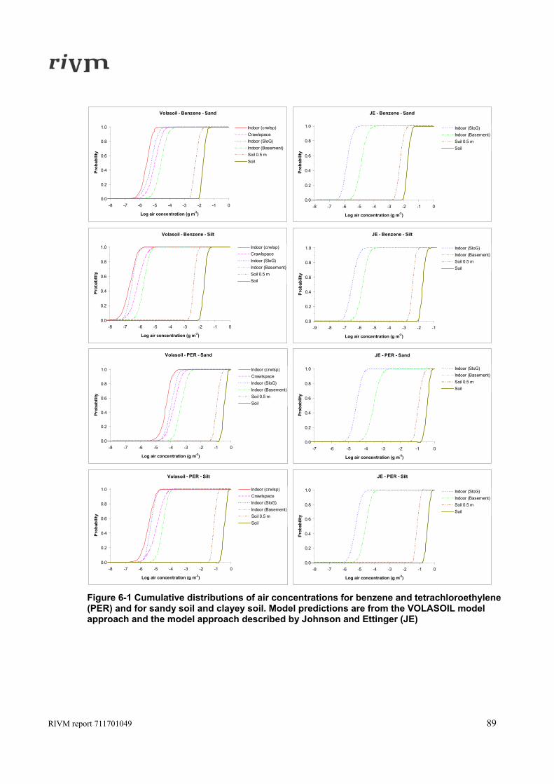
RIVM report 711701049 89
Volasoil - Benzene - Silt
0.0
0.2
0.4
0.6
0.8
1.0
-8 -7 -6 -5 -4 -3 -2 -1 0
Log air concentration (g m-3)
Prob
abili
ty
Indoor (crwlsp)CrawlspaceIndoor (SloG)Indoor (Basement)Soil 0.5 mSoil
Volasoil - PER - Sand
0.0
0.2
0.4
0.6
0.8
1.0
-8 -7 -6 -5 -4 -3 -2 -1 0
Log air concentration (g m-3)
Prob
abili
ty
Indoor (crwlsp)CrawlspaceIndoor (SloG)Indoor (Basement)Soil 0.5 mSoil
Volasoil - PER - Silt
0.0
0.2
0.4
0.6
0.8
1.0
-8 -7 -6 -5 -4 -3 -2 -1 0
Log air concentration (g m-3)
Prob
abili
ty
Indoor (crwlsp)CrawlspaceIndoor (SloG)Indoor (Basement)Soil 0.5 mSoil
JE - PER - Sand
0.0
0.2
0.4
0.6
0.8
1.0
-7 -6 -5 -4 -3 -2 -1 0
Log air concentration (g m-3)
Prob
abili
ty
Indoor (SloG)Indoor (Basement)Soil 0.5 mSoil
JE - Benzene - Sand
0.0
0.2
0.4
0.6
0.8
1.0
-8 -7 -6 -5 -4 -3 -2 -1 0
Log air concentration (g m-3)
Prob
abili
ty
Indoor (SloG)Indoor (Basement)Soil 0.5 mSoil
JE - PER - Silt
0.0
0.2
0.4
0.6
0.8
1.0
-8 -7 -6 -5 -4 -3 -2 -1 0
Log air concentration (g m-3)
Prob
abili
ty
Indoor (SloG)Indoor (Basement)Soil 0.5 mSoil
JE - Benzene - Silt
0.0
0.2
0.4
0.6
0.8
1.0
-9 -8 -7 -6 -5 -4 -3 -2 -1
Log air concentration (g m-3)
Prob
abili
ty
Indoor (SloG)Indoor (Basement)Soil 0.5 mSoil
Volasoil - Benzene - Sand
0.0
0.2
0.4
0.6
0.8
1.0
-8 -7 -6 -5 -4 -3 -2 -1 0
Log air concentration (g m-3)
Prob
abili
ty
Indoor (crwlsp)CrawlspaceIndoor (SloG)Indoor (Basement)Soil 0.5 mSoil
Figure 6-1 Cumulative distributions of air concentrations for benzene and tetrachloroethylene (PER) and for sandy soil and clayey soil. Model predictions are from the VOLASOIL model approach and the model approach described by Johnson and Ettinger (JE)
90 RIVM report 711701049
6.3.2.1 Gaps and holes approach In general the results of the uncertainty analysis for each modelling approach (VOLASOIL and Johnson and Ettinger) and the various combinations of substance and soil type is very alike. The calculated concentration decreases from the highest concentration in indoor air for the basement, to the concentration in the crawl space air, next the indoor air concentration for the slab on grade building type and finally the lowest concentration in indoor air for the building type with a crawl space, see also Figure 6-1. The higher concentration in indoor air for a building with a basement results from different aspects. For this building type the soil column is reduced (floor is closer to contamination) and therefore there is less resistance to transport through the soil. Secondly the effective surface area of the basement through which transport takes place is larger because the basement wall area is included in addition to the floor area. The indoor air concentration for the slab on grade scenario lies between the concentration in the crawl space air and indoor air for the crawl space scenario. This seems sound as the crawl space can be seen as a removal route, through the crawl space ventilation, which is absent in the slab on grade scenario. The difference between the concentration in indoor air and crawl space air is about a factor of 5, which is in line with the results presented by Van Wijnen and Lijzen (2006). This ratio is decreasing though for silty soil. This can be explained by the limiting influence of convective transport as silty soils are less permeable than sandy soils. Diffusive transport plays a more important role in the scenarios for silty soil. This seems to be a general picture for the differences between the various building types, though less pronounced. The difference between the indoor concentration for a building with crawl space and a building with a basement is approximately about a factor of 10. 6.3.2.2 Johnson and Ettinger approach For the Johnson and Ettinger approach only the slab on grade scenario and the basement scenario can be compared (Figure 6-1). The picture is rather consistent for the both substances and soil types. As can be expected, the concentration in indoor air for the building with basement is higher, about a factor of 10. There seems to be no clear difference between the results for both soil types. Only the indoor concentrations for silt are lower due to limited convective transport. 6.3.2.3 Modelling approach, intercomparison The results of the two modelling approaches are presented in Figure 6-2 and seem to be well in line with each other, the difference is less than a factor of three. The Johnson and Ettinger approach calculates a lower concentration in the case of a sandy soil type. The predicted indoor concentrations are almost the same for the silt soil type. This indicates that the air permeability of soil is a more sensitive parameter and has a larger contribution for the VOLASOIL approach. There is no difference in the results for the two substances.
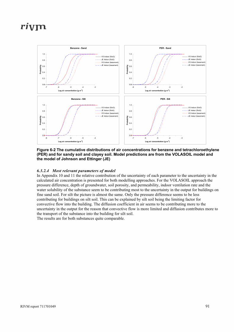
RIVM report 711701049 91
Benzene - Sand
0.0
0.2
0.4
0.6
0.8
1.0
-7 -6 -5 -4 -3
Log air concentration (g m-3)
Prob
abili
ty
VS Indoor (SloG)JE Indoor (SloG)VS Indoor (basement)JE Indoor (basement)
PER - Sand
0.0
0.2
0.4
0.6
0.8
1.0
-6 -5 -4 -3 -2
Log air concentration (g m-3)
Prob
abili
ty
VS Indoor (SloG)JE Indoor (SloG)VS Indoor (basement)JE Indoor (basement)
Benzene - Silt
0.0
0.2
0.4
0.6
0.8
1.0
-8 -7 -6 -5 -4
Log air concentration (g m-3)
Prob
abili
ty
VS Indoor (SloG)JE Indoor (SloG)VS Indoor (basement)JE Indoor (basement)
PER - Silt
0.0
0.2
0.4
0.6
0.8
1.0
-7 -6 -5 -4 -3
Log air concentration (g m-3)
Prob
abili
ty
VS Indoor (SloG)JE Indoor (SloG)VS Indoor (basement)JE Indoor (basement)
Figure 6-2 The cumulative distributions of air concentrations for benzene and tetrachloroethylene (PER) and for sandy soil and clayey soil. Model predictions are from the VOLASOIL model and the model of Johnson and Ettinger (JE)
6.3.2.4 Most relevant parameters of model In Appendix 10 and 11 the relative contribution of the uncertainty of each parameter to the uncertainty in the calculated air concentration is presented for both modelling approaches. For the VOLASOIL approach the pressure difference, depth of groundwater, soil porosity, and permeability, indoor ventilation rate and the water solubility of the substance seem to be contributing most to the uncertainty in the output for buildings on fine sand soil. For silt the picture is almost the same. Only the pressure difference seems to be less contributing for buildings on silt soil. This can be explained by silt soil being the limiting factor for convective flow into the building. The diffusion coefficient in air seems to be contributing more to the uncertainty in the output for the reason that convective flow is more limited and diffusion contributes more to the transport of the substance into the building for silt soil. The results are for both substances quite comparable.
92 RIVM report 711701049
6.4 Conclusion From the uncertainty analysis it can be concluded that the differences in calculated concentrations can be explained and are logical. The concentrations in a house with a basement are higher due to the closer distance to the contaminants and a larger contact area between the building and the underlying soil. Besides, it is also clear that there is a partial overlap between the scenarios. The contribution to the output uncertainty seems largely based on substance properties (solubility and vapour pressure), soil properties (permeability, depth of the groundwater and porosity), and building characteristics (pressure difference, ventilation rate, floor area). Compared to the sensitivity analysis, the uncertainty in the groundwater concentration and building parameters like the floor area are not considered, although being sensitive parameters with respect to the model output. Again it is important to note that the sensitivity of the model parameters in relation to model output and the uncertainty in the model output depends on the default model parameter value setting. Other model settings will lead to different results. The overcome this and illustrate the effect of different model settings different scenarios based on two different soil types and two different substances were considered in the uncertainty analysis. From the results it can be concluded that for site specific risk assessment the focus should be on obtaining reliable soil or ground water concentrations and proper estimation of the soil type or measured values of the permeability, porosity of the subsoil and the depth of the groundwater table. Additionally, structure related parameters like the pressure difference and the ventilation rate are important in obtaining sound modelling results.
RIVM report 711701049 93
7. Conclusions and recommendations Within the framework of human risk assessment of soil and groundwater contamination, human exposure modelling with site specific information is the second step (tier 2) after exceeding intervention values of soil and/ or groundwater has been determined. The third step (tier 3) is the use of site specific measurements for risk assessment. For the risk assessment of volatile compounds the same steps have been followed. Because of the conservative, approach, calculated air concentrations will, probably in more than half of the cases overestimate the measured indoor air concentration. In a step-wise procedure this is a functional element that prevents that there is a substantial chance that a lower step is less conservative than a higher step in the risk assessment with more site specific data. Compared to the earlier model concepts for the risk assessment of volatile compounds two additional building scenarios are added: slab-on-grade buildings and buildings with a basement. Calculations for these building types are now also possible. where in the past no calculations could be done or wrong calculations were done based on the scenario ‘building with a crawlspace’. In addition to the new building types two new modelling approaches have been introduced. The previous VOLASOIL model was based on modelling laminar flow the straight tubes. The modelling of indoor air concentrations has now been extended with two other approaches, which represent different situations in practice. The perimeter seam gap approach (1) is commonly used for buildings with a slab on grade floor and residences with a basement. It best fits the situation where there is a gap between the foundation (floor) and the walls. Furthermore, the porous media approach (2) was introduced. This approach is most appropriate to the situation of newly build modern residences with the floor and wall constructed as one piece using high quality concrete. The introduction of the additional building types and modelling approaches introduces more complexity and puts higher demands on the knowledge of residence construction and assessment of the actual situation. On the other hand the modelling extensions provide the possibility of more realistic and accurate assessment of indoor air concentrations at contaminated sites. Thirdly more insight is given in de relevance of the values of the model parameters. The (default) value of some parameters (e.g. area of opening in the floor, pressure difference between soil and crawlspace) has been changed in order to slightly reduce the calculated concentration in indoor air, which is more in line with field observations. Also some other improvements have been implemented, for instance the dependency of the volume fraction of air and water in soil on the soil type, additional floor quality types and using the air exchange rate instead of the ventilation rate. It is recommended to implement these new scenarios in the instrumentation of the second step of the Remediation Criteria. In the third step of the remediation criteria the full opportunities of the modelling, including the alternative model concepts can be incorporated. It is recommended to update the VOLASOIL model with these new scenarios and model concepts in order to facilitate these risk assessment. It is identified that modelling of indoor air concentrations based on soil and groundwaterconcentrations has limitations. Therefore it is recommended to carry out measurements when, based on these calculations, criteria are exceeded or indoor air is influenced by the contamination. Both modelling and measurement are important for the risk assessment and decisions on remediation.

94 RIVM report 711701049
RIVM report 711701049 95
References Aldenkamp FJ, Stoop P. 1994. Sources and transport of indoor radon: measurements and
mechanisms. Rijksuniversiteit Groningen.
Andersen CE, Bergsoe NC, Majborn B, Ulbak K. 1997. Radon and natural ventilation in newer Danish single-family houses. Indoor Air 7: 278-286.
Andrade C, Sagrera JL, Martinez I, Garcia M and Zuloaga P. 2003. Monitoring of Concrete Permeability, Carbonation and Corrosion Rates in the Concrete of the Containers of El Cabril (Spain) Disposal. Transactions of the 17th International Conference on Structural Mechanics in Reactor Technology (SMiRT 17). Prague, Czech Republic, August 17-22.
Arnold LJ. 1990. A scale model study of the effects of meteorological, soil, and house parameters on soil gas pressures. Health Physics 58 (5): 559-537.
Baars, A.J., Theelen R.M.C., Janssen P.J.C.M., Hesse J.M., Van Apeldoorn M.E., Meijerink M.C.M., Verdam L., and Zeilmaker M.J. (2001): Re-evaluation of human-toxicological maximum permissible risk levels. Bilthoven, The Netherlands: National Institute for Public Health and the Environment (RIVM). RIVM report no. 711701025.
Bakker H de, Schelling J. 1986. Systeem van bodemclassificatie voor Nederland; de hogere niveaus, 2nd ed. Pudoc, Wageningen, the Netherlands.
Bentz DP, Quenard DA, Kunzel HM, Baruchel J, Peyrin F, Martys NS and Garboczi EJ. 2000, Microstructure and transport properties of porous building materials. II: Three-dimensional X-ray tomographic studies. Materials and Structures 33: 147-153.
Brown DG, Gupta L, Kim T-H, Moo-Young HK and Coleman AJ. 2006. Comparative assessment of coal tars obtained from 10 former manufactured gas plant sites in the Eastern United States. Chemosphere 65: 1562-1569.
Chevron 2007. Crude Oil Marketing. Assay data tables for various properties across a standard set of crude cuts. Available at: http://crudemarketing.chevron.com/ site_index.asp
Denarié E. 2003. Application of in-sity quality control of cover concrete. Methodology and requirements. Laboratory of Maintenance and Safety of Structures (MCS), Institute of Structures (IS)
Dolomatov MY, Khashper LM and Kuz’mina ZF. 1991. Spectroscopic method for determination of the average molecular weight. Chemistry and Technology of Fuels and Oils 27 (7): 401-403.
EA. 2002. The Contaminated Land Exposure Assessment (CLEA) Model: Technical Basis and Algorithms. Bristol, United Kingdom: The Environment Agency (EA), Department of Environment, Food and Rural Affairs.
FAO. 1990. Guidelines for soil profile description; 3rd edition (revised). Soil Resources, Management and Conservation Service, Land and Water Management Devision. Rome.
Fast T, Kliest J, van de Wiel H. 1987. De bijdrage van bodemverontreiniging aan de verontreiniging van de lucht in woningen. Ministery van Volkshuisvesting, Ruimtelijke Ordening en Milieubeheer (VROM). Publikatiereeks Milieubeheer nr. 6.
Ferguson, C.C., Krylov, V.v., and McGrath, P.T., (1995). Contamination of Indoor Air by Toxic Soil Vapours: a Screening Assessment Model. Building and Environment 30(3): 375-383.
96 RIVM report 711701049
Fugler D and Adomait M. 1997. Indoor infiltration of volatile organic contaminants: measured soil gas entry rates and other results fo Canadian houses. Journal of soil contamination 6(1): 9-13.
Garbesi K, Sextro RG. 1989. Modelling and Field Evidence of Pressure-Driven Entry of Soil Gas into House through Permeable Below-Grade Walls. Environmental Science and Technology 23(12): 1481-1487.
Garbesi K, Sextro RG. et al. 1993. Soil-gas entry into an experimental basement: model measurement comparisons and seasonal effects. Environmental Science and Technology 23(12): 1481-1487.
Gilyazetdinov LP. 1992. Calculation of Molecular Weight of Fractions of Hydrocarbon Stocks. Chemistry and Technology of Fuels and Oils 28 (9): 530-532.
Hansen BE, Malmros O, Turner NR, Stenby EH and Andersen SI. 2002. Size Exclusion Chromatography in the Analysis of Pitch. Available at http://www.koppers.com/htm/PandS_RanD_WhiteP.html
Hazebrouck B, Gay G, Hulot C. 2005. Vapour Emissions from Contaminated Soils into Buildings: Developments of the Volasoil for a Multilayer Soil.Paper presented at Consoil 2005.
Health Council of the Netherlands. 2004. Risks of soil contaminants for human health: soil testing procedures, models, standards. The Hague: Health Council of the Netherlands, 2004. Publication no 2004/15
Hers I, Zapf-Gilje R, Li L and Atwater J. 2001. The use of indoor air measurements to evaluate intrusion of subsurface VOC vapors into buildings. Journal of the Air and Waste Management Association 51(9): 1318-1331.
Hintenlang DE, and Al-Ahmandy KK. 1992. Pressure differences for radon entry coupled to periodic atmospheric pressure variations. Indoor Air 2: 208-215.
Janssen MPM, de Vries L, Phaff JC, van der Graaf ER, Blaauboer RO, Stoop P, Lembrechts J. 1998. Modelling radon transport in Dutch dwellings. Bilthoven, the Netherlands: National Institute for Public Health and the Environment (RIVM). RIVM report no. 610050005.
Janssen PHM, Heuberger PSC, Sanders R. 1992. UNCSAM 1.1: A Software Package for Sensitivity and Uncertainty Analysis. Manual. Bilthoven, the Netherlands: National Institute for Public Health and the Environment (RIVM). RIVM report no. 959101004.
Johnson PC, Ettinger RA. 1991. Heuristic Model for Predicting the Intrusion Rate of Contaminant Vapours into Buildings. Environmental Science and Technology 25: 1445-1452.
Koorevaar P, Menelik G, Dirksen C. 1983. Elements of soil physics. Developments in soil science 13. Amsterdam, Elsevier.
Krylov VV, Ferguson CC. 1998. Contamination of Indoor Air by Toxic Soil Vapours: Effects of Subfloor Ventilation and Other Protective Measures. Building and Environment 33(6): 331-347.
Lide DR, et al. 1993. CRC Handbook of Chemistry and Physics, 74th edition, 1993-1994. CRC Press, Boco Raton, FL.
Lijzen JPA, Baars AJ, Otte PF, Rikken MGJ, Swartjes FA, Verbruggen EMJ, Van Wezel AP. 2001. Technical evaluation of the Intervention Values for Soil/sediment and Groundwater. Bilthoven, the Netherlands: National Institute for Public Health and the Environment (RIVM). RIVM report no. 711701023.
RIVM report 711701049 97
Lijzen JPA, Otte PF, Kovar K, et al. 2003. Progress report Evaluation of the Remediation Urgency Methodology; analysis of restraints and first exploration of solutions. Bilthoven, the Netherlands: National Institute for Public Health and the Environment (RIVM). RIVM report no. 711701033.
Lijzen J.P.A., P.F. Otte, J. Bakker, F.A. Swartjes, A.J. Baars, A.G. Oomen and E. Brand. 2008, in prep. Guidance for site-specific human-toxicological risk assessment of soil contamination. Bilthoven, the Netherlands: National Institute for Public Health and the Environment (RIVM). RIVM report no. 711701050.
Loureiro CO, Abriola LM, Martin JE, Sextro RG. 1990. Three-Dimensional Simulation of Radon Transport into House with Basements under Constant Negative Pressure. Environmental Science and Technology 24(9): 1338-1348.
Mackay D, Shiu WY, Ma KC. 1992a. Illustrated handbook of physical-chemical properties and environmental fate for organic chemicals. Vol 1: monoaromatic hydrocarbons, chlorobenzenes and PCBs.
Mackay D, Shiu WY, Ma KC. 1992b. Illustrated handbook of physical-chemical properties and environmental fate for organic chemicals. Vol 3: volatile organic chemicals.
McCarthy KP and Brown KW. 1992. Soil Gas Permeability as influenced by Soil Gas-Filled Porosity. Soil Science Society of America 56(4): 997-1003.
Mowris RJ and Fisk WJ. 1988. Modelling the effects of exhaust ventilation on radon entry rates and indoor radon concentrations. Health Physics 54(5): 491-501.
Nazaroff WW et al. 1985. Radon transport into a detached one-story house with basement. Atmospheric Environment 19(1): 41-46.
Nazaroff, WW. 1988. Predicting the Rate of 222Rn Entry from Soil into the Basement of a Dwelling due to Pressure-driven Air Flow. Radiation Protection Dosimetry 24: 199-202.
Nielson KK, Rogers VC, Holt RB, Pugh TD, Grondzik WA and Meijer RJ. 1997. Radon Penetration of Concrete Slab Cracks, Joints, Pipe Penetrations, and Sealants. Health Physics Society 73(4): 668-678.
NNI. 1989. Geotechniek - Classificatie van onverharde grondmonsters. NEN 5104:1989/C1:1990 nl, Nederlandse Normalisatie Instituut (NNI)
Oomen AG, Brandon EFA, Swartjes FA, Sips AJAM. 2006. How can information on oral bioavailability improve human health risk assessment for lead-contaminated soils? Implementation and scientific basis. Bilthoven, the Netherlands: National Institute for Public Health and the Environment (RIVM). RIVM report no. 711701042.
Otte, P.F., JPA Lijzen, JG Otte, FA Swartjes, Versluijs CW. 2001. Evaluation and revision of the CSOIL parameter set. Proposed parameter set for human exposure modelling and deriving Intervention Values for the first series of compounds. Bilthoven, the Netherlands: National Institute for Public Health and the Environment (RIVM). RIVM report no.711701021, pp.125.
Otte PF, Lijzen JPA, Mennen MG, Spijker J. 2007. Guidance on air quality measurement for assessing risks of contaminated soil. Bilthoven, the Netherlands: National Institute for Public Health and the Environment (RIVM). RIVM report no. 711701048. (In Dutch).
Özel MZ, Bartle KD. 2001. Production of Mesophase Pitch from Coal Tar and Petroleum Pitches using Supercritical Fluid Extraction. Turkish Journal of Chemistry. 26: 417-424.
98 RIVM report 711701049
Poels CLM, Gruntz U, Isnard P, Riley D, Piteller M, ten Berge W, Veerkamp W, Bontinck WJ. 1990. ECETOC technical report nr. 40, Hazard Assessment of Chemical Contaminants in Soil.
Put LW, de Meijer RJ. 1989. Luchtdrukverschillen in en rond woningen: implicaties voor het transport van radon. Air pressure differences in and around residences: implications for the transport for radon (in Dutch). Kernfysisch Versneller Instituut, Universiteit Groningen, Nederland.
Quikrete. 2007. Information Sheet on Slab foundations. Concrete Foundations. Available at: http://www.quikrete.com/AtHome/Building.asp:
Rikken MGJ, Lijzen JPA, Cornelese AA. 2001. Evaluation of model concepts on human exposure; Proposals for updating the most relevant exposure routes of CSOIL. Bilthoven, the Netherlands: National Institute for Public Health and the Environment (RIVM). RIVM report no. 711701022.
Robinson AL and Sextro RG. 1995a. The influence of a subslab gravel layer and open area on soil-gas and radon entry into two experimental basements. Health Physics 69(3): 367-377.
Robinson AL and Sextro RG. 1995b. Direct measurements of soil gas entry into and experimental basement driven by atmospheric pressure fluctuations, Lawrence Berkeley Laboratory, University of California, Energy and Environmental Division.
Roy DM, Brown PW, Ski D, Scheetz BE, May W. 1993. Concrete Microstructure Porosity and Permeability. Materials Research Laboratory, The Pennsylvania State University, University Park, Pennsylvania. Strategic Highway Research Program, National Research Council, Washington, DC 1993.
Scott AG. 1992. Site characterization for radon supply potential: A progress review. Health Physics, 62 (5): 422-428.
Shell Global Solutions 1995. The concepts of HESP. Reference Manual, Human Exposure to Soil Pollutants, version2.10b. Jan 1995.Sextro RG, Moed BA, Nazaroff WW, Revzan KL, Nero AV, (1986). Investigations of soil as a source of indoor radon. Lawrence Berkely Laboratory, Berkeley CA. LBL-21572.
Stoop P, Galstra P, Hiemstra Y, de Vries L and Lembrechts J. 1998. Results of the second Dutch national survey on radon in dwellings. Bilthoven, the Netherlands: National Institute for Public Health and the Environment (RIVM). RIVM report no. 610058006.
Swartjes, FA. 1999 Risk based assessment of Soil and Groundwater Quality in the Netherlands: Standards and Remediation Urgency. Risk Analyses, Vol. 19, No. 6, 1235-1249
Swartjes FA, Dirven-van Breemen EM, Otte PF, Beelen P van, Rikken MGJ, Tuinstra J, Spijker J, Lijzen JPA. 2007. Towards a protocol for the assessment of site-specific human health risks for consumption of vegetables from contaminated sites. Bilthoven, the Netherlands: National Institute for Public Health and the Environment (RIVM). RIVM report no. 711701040.
TCB. 2002. Advies Wetenschappelijke evaluatie interventiewaarden. TCB A31 (2002). Den Haag, juli 2002.
US-DE. 2003. Technology Fact Sheet: ‘Slab Insulation’. United States Department of Energy (US-DE) Office of Building Technology, State and Community Programs Energy Efficiency and Renewable Energy.
US-EPA. 2003. USER'S GUIDE FOR EVALUATING SUBSURFACE VAPOR INTRUSION INTO. United States Environmental Protection Agency (US-EPA) office of emergency and remedial response.
RIVM report 711701049 99
US-EPA. 2006. Diffusion Coefficient Estimation Tool. United States Environmental Protection Agency (US-EPA). Available at: http://www.epa.gov/athens/learn2model/part-two/onsite/estdiffusion-ext.htm
US-EPA. 2007. EPA On-line Tools for Site Assessment Calculations, Effective Solubility Calculator. United State Environmental Protection Agency (US-EPA). Avialable at: http://www.epa.gov/athens/learn2model/part-two/onsite/es.htm
Van Dongen J. and VOS H. 2007. Gezondheidsaspecten van woningen in Nederland. Delft, the Netherlands: TNO Leefomgeving en Beleid, TNO Bouw en Ondergrond. TNO report 2007-D-R 0188/A.
Van Veen MP, Crommentuijn LEM, Janssen MPM, de Hollander AEM. 2001. Binnenmilieu-kwaliteit: ventilatie en vochtigheid. Een studie voor milieuverkenning 5 Bilthoven, the Netherlands: National Institute for Public Health and the Environment (RIVM). RIVM report no. 630920 001.
Van Wijnen HJ and Lijzen JPA. 2006. Validation of the VOLASOIL model using air measurements from Dutch contaminated sites. Bilthoven, the Netherlands: National Institute for Public Health and the Environment (RIVM). RIVM report no. 711701401.
VROM 1995. Koolenbrander J. Urgentie van bodemsanering: de handleiding. SDU, Den Haag.
VROM 1998. Circulaire Saneringsregeling Wet bodembescherming: beoordeling en afstemming. Circulaire van 19 december 1997, kenmerk DBO/97587346.
VROM, 2000. Ministerial Circular on Target and Intervention soil remediation ( in Dutch: ‘Circulaire streef- en interventiewaarden bodemsanering’ Referentie DBO/1999226863.
VROM 2003a. Beleidsbrief Bodem. Referentie BWL/2003 096 250, december 2003.
VROM 2003b.Publicatiereeks Gevaarlijke Stoffen 1. Deel 5: Bescherming tegen toxische stoffen door verblijf binnenshuis, december 2003.
VROM 2005. Praktijkboek Bouwbesluit 2003. VROM Directoraat-Generaal Wonen, Den Haag, the Netherlands.
VROM, 2006. Circulaire Bodemsanering 2006. Staatscourant 28 april 2006, nr 38 pag 34.
Waitz MFW, Freijer JI, Kreule P, Swartjes FA. 1996. The VOLASOIL risk assessment model based on CSOIL for soils contaminated with volatile compounds. Bilthoven, the Netherlands: National Institute for Public Health and the Environment (RIVM). RIVM report no. 715810014.
Wösten JHM, Veerman GJ, De Groot WJM, Stolte J. 2001. Waterretentie- en doorlatendheidskarakteristieken van boven- en ondergronden in Nederland: de Staringsreeks. alterra-rapport No. 153, Vernieuwde uitgave. wageningen, the Netherlands, Alterra Research Instituut voor de Groen Ruimte.
Zulovich JM. 2005. Concrete Basement Construction. Department of Agricultural Engineering. Available at: http://muextension.missouri.edu/xplor/aggguides/agengin/g01700.htm. Date: 20-10-2005.

100 RIVM report 711701049
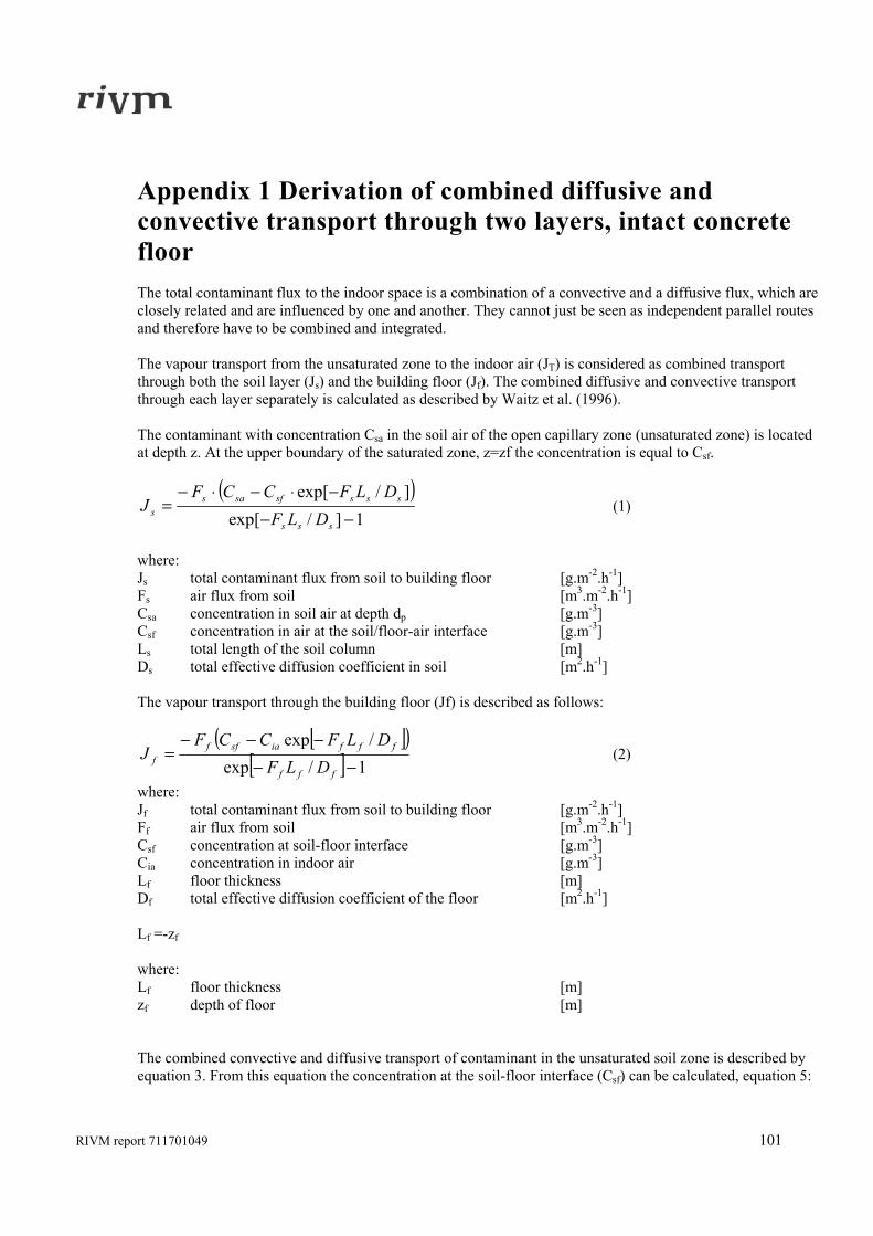
RIVM report 711701049 101
Appendix 1 Derivation of combined diffusive and convective transport through two layers, intact concrete floor The total contaminant flux to the indoor space is a combination of a convective and a diffusive flux, which are closely related and are influenced by one and another. They cannot just be seen as independent parallel routes and therefore have to be combined and integrated. The vapour transport from the unsaturated zone to the indoor air (JT) is considered as combined transport through both the soil layer (Js) and the building floor (Jf). The combined diffusive and convective transport through each layer separately is calculated as described by Waitz et al. (1996). The contaminant with concentration Csa in the soil air of the open capillary zone (unsaturated zone) is located at depth z. At the upper boundary of the saturated zone, z=zf the concentration is equal to Csf.
( )1]/exp[
]/exp[−−
−⋅−⋅−=
sss
ssssfsass DLF
DLFCCFJ (1)
where: Js total contaminant flux from soil to building floor [g.m-2.h-1] Fs air flux from soil [m3.m-2.h-1] Csa concentration in soil air at depth dp [g.m-3] Csf concentration in air at the soil/floor-air interface [g.m-3] Ls total length of the soil column [m] Ds total effective diffusion coefficient in soil [m2.h-1] The vapour transport through the building floor (Jf) is described as follows:
[ ]( )[ ] 1/exp
/exp−−
−−−=
fff
fffiasfff DLF
DLFCCFJ (2)
where: Jf total contaminant flux from soil to building floor [g.m-2.h-1] Ff air flux from soil [m3.m-2.h-1] Csf concentration at soil-floor interface [g.m-3] Cia concentration in indoor air [g.m-3] Lf floor thickness [m] Df total effective diffusion coefficient of the floor [m2.h-1] Lf =-zf where: Lf floor thickness [m] zf depth of floor [m] The combined convective and diffusive transport of contaminant in the unsaturated soil zone is described by equation 3. From this equation the concentration at the soil-floor interface (Csf) can be calculated, equation 5:
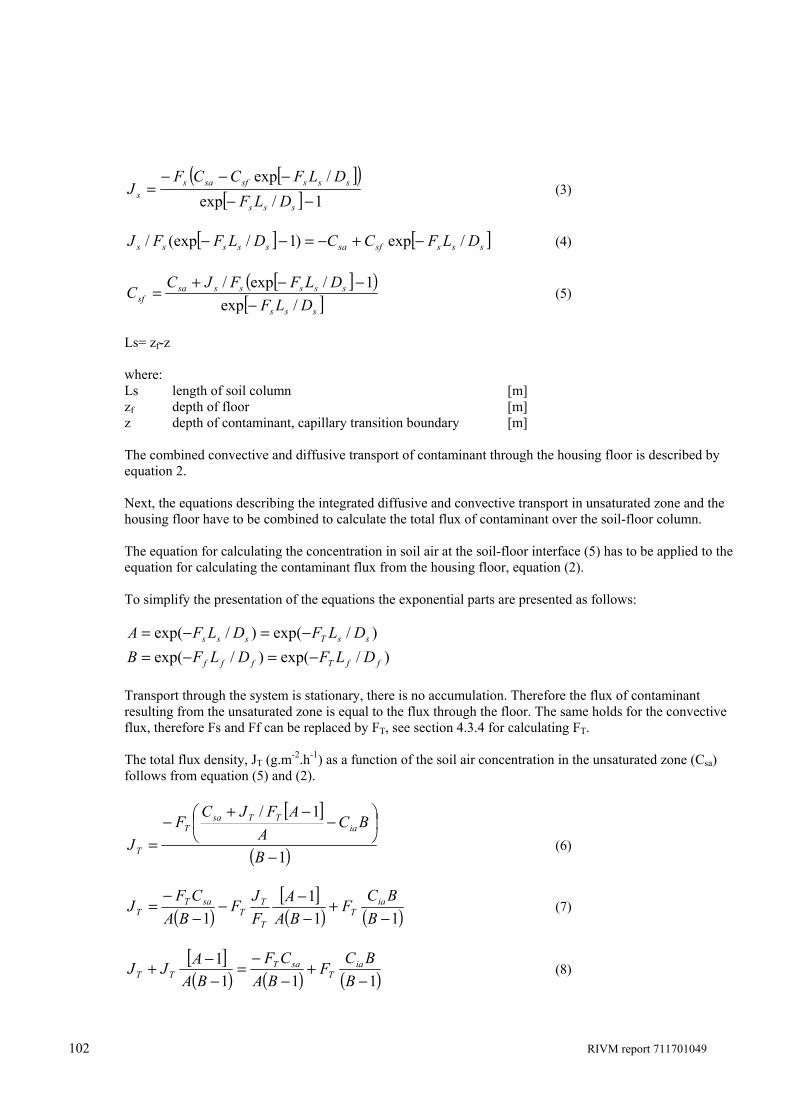
102 RIVM report 711701049
[ ]( )
[ ] 1/exp/exp
−−−−−
=sss
ssssfsass DLF
DLFCCFJ (3)
[ ] [ ]ssssfsasssss DLFCCDLFFJ /exp)1/(exp/ −+−=−− (4)
[ ]( )
[ ]sss
ssssssasf DLF
DLFFJCC
/exp1/exp/
−−−+
= (5)
Ls= zf-z where: Ls length of soil column [m] zf depth of floor [m] z depth of contaminant, capillary transition boundary [m] The combined convective and diffusive transport of contaminant through the housing floor is described by equation 2. Next, the equations describing the integrated diffusive and convective transport in unsaturated zone and the housing floor have to be combined to calculate the total flux of contaminant over the soil-floor column. The equation for calculating the concentration in soil air at the soil-floor interface (5) has to be applied to the equation for calculating the contaminant flux from the housing floor, equation (2). To simplify the presentation of the equations the exponential parts are presented as follows:
)/exp()/exp()/exp()/exp(
ffTfff
ssTsss
DLFDLFBDLFDLFA
−=−=−=−=
Transport through the system is stationary, there is no accumulation. Therefore the flux of contaminant resulting from the unsaturated zone is equal to the flux through the floor. The same holds for the convective flux, therefore Fs and Ff can be replaced by FT, see section 4.3.4 for calculating FT. The total flux density, JT (g.m-2.h-1) as a function of the soil air concentration in the unsaturated zone (Csa) follows from equation (5) and (2).
[ ]
( )1
1/
−
⎟⎠⎞
⎜⎝⎛ −
−+−
=B
BCA
AFJCF
Jia
TTsaT
T (6)
( )[ ]( ) ( )11
11 −
+−
−−−
−=
BBC
FBA
AFJ
FBA
CFJ ia
TT
TT
saTT (7)
[ ]( ) ( ) ( )111
1−
+−
−=
−−+
BBC
FBA
CFBA
AJJ iaT
saTTT (8)
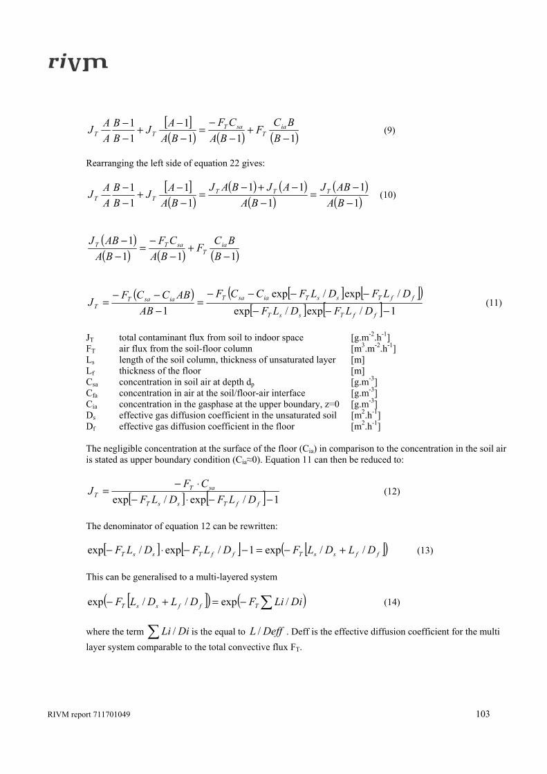
RIVM report 711701049 103
[ ]( ) ( ) ( )111
111
−+
−−
=−
−+−−
BBC
FBA
CFBA
AJBB
AAJ ia
TsaT
TT (9)
Rearranging the left side of equation 22 gives:
[ ]( )
( ) ( )( )
( )( )1
11
111
111
−−
=−
−+−=
−−+
−−
BAABJ
BAAJBAJ
BAAJ
BB
AAJ TTT
TT (10)
( )( ) ( ) ( )111
1−
+−
−=
−−
BBC
FBA
CFBAABJ ia
TsaTT
( ) [ ] [ ]( )[ ] [ ] 1/exp/exp
/exp/exp1 −−−
−−−−=
−−−
=ffTssT
ffTssTiasaTiasaTT DLFDLF
DLFDLFCCFAB
ABCCFJ (11)
JT total contaminant flux from soil to indoor space [g.m-2.h-1] FT air flux from the soil-floor column [m3.m-2.h-1] Ls length of the soil column, thickness of unsaturated layer [m] Lf thickness of the floor [m] Csa concentration in soil air at depth dp [g.m-3] Cfa concentration in air at the soil/floor-air interface [g.m-3] Cia concentration in the gasphase at the upper boundary, z=0 [g.m-3] Ds effective gas diffusion coefficient in the unsaturated soil [m2.h-1] Df effective gas diffusion coefficient in the floor [m2.h-1] The negligible concentration at the surface of the floor (Cia) in comparison to the concentration in the soil air is stated as upper boundary condition (Cia≈0). Equation 11 can then be reduced to:
[ ] [ ] 1/exp/exp −−⋅−⋅−
=ffTssT
saTT DLFDLF
CFJ (12)
The denominator of equation 12 can be rewritten:
[ ] [ ] [ ]( )ffssTffTssT DLDLFDLFDLF //exp1/exp/exp +−=−−⋅− (13) This can be generalised to a multi-layered system
[ ]( ) ( )∑−=+− DiLiFDLDLF TffssT /exp//exp (14) where the term ∑ DiLi / is the equal to DeffL / . Deff is the effective diffusion coefficient for the multi layer system comparable to the total convective flux FT.
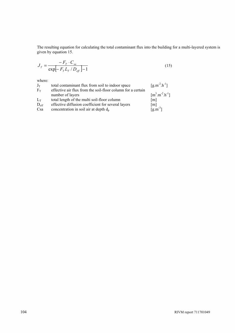
104 RIVM report 711701049
The resulting equation for calculating the total contaminant flux into the building for a multi-layered system is given by equation 15.
[ ] 1/exp −−⋅−
=effTT
saTT DLF
CFJ (15)
where: JT total contaminant flux from soil to indoor space [g.m-2.h-1] FT effective air flux from the soil-floor column for a certain number of layers [m3.m-2.h-1] LT total length of the multi soil-floor column [m] Deff effective diffusion coefficient for several layers [m] Csa concentration in soil air at depth dp [g.m-3]
RIVM report 711701049 105
Appendix 2 Derivation of combined diffusive and convective transport through two layers, floor with cracks and gaps or a perimeter seam gap Combined diffusive and convective transport through two (porous) layers. The vapour transport from the unsaturated zone to the indoor air (J) is considered as combined transport through both the soil layer (Js) and the building floor (Jf). The combined diffusive and convective transport through each layer separately is calculated as described by Waitz et al. (1996). The contaminant with concentration Csa in the soil air of the open capillary zone (unsaturated zone) is located at depth z. At the upper boundary of the saturated zone, z=zf the concentration is equal to Csf.
( )1]/exp[
]/exp[−−
−⋅−⋅−=
sss
ssssfsass DLF
DLFCCFJ (1)
where: Js total contaminant flux from soil to building floor [g.m-2.h-1] Fs air flux from soil [m3.m-2.h-1] Csa concentration in soil air at depth dp [g.m-3] Csf concentration in air at the soil/floor-air interface [g.m-3] Ls total length of the soil column [m] Ds total effective diffusion coefficient in soil [m2.h-1] The vapour transport through the building floor (Jf) is described as follows:
[ ]( )[ ] 1/exp
/exp−−
−−−=
fff
fffiasfff DLF
DLFCCFJ (2)
where: Jf total contaminant flux from soil to building floor [g.m-2.h-1] Ff air flux from soil [m3.m-2.h-1] Csf concentration at soil-floor interface [g.m-3] Cia concentration in indoor air [g.m-3] Lf floor thickness [m] Df total effective diffusion coefficient of the floor [m2.h-1] Lf =-zf where: Lf floor thickness [m] zf depth of floor [m] The concentration at the soil-floor interface (Csf) can be calculated as follows, see also Appendix 1:
[ ]( )[ ]sss
ssssssasf DLF
DLFFJCC
/exp1/exp/
−−−+
= (3)
106 RIVM report 711701049
Ls= zf-z where: Ls length of soil column [m] zf depth of floor [m] z depth of contaminant, capillary transition boundary [m] Next, the equations describing the integrated diffusive and convective transport in unsaturated zone and the housing floor have to be combined to calculate the total flux of contaminant over the soil-floor column, as in Appendix 1. Gaps and holes in the floor (VOLASOIL concept) In the specific case of transport through the cracks and gaps in the floor, the convective flux and diffusive transport should be based on the cracks and gaps and not on the floor as a whole. As, transport through the system is stationary, there is no accumulation. Therefore the total flux of contaminant resulting from the unsaturated zone is equal to the flux through the floor. The same holds for the convective flux. From this it can be assumed that Fs and Ff are related through:
f
gapfs A
AJJ = (4)
where: Acrack area of cracks or holes in the floor [m2] Af cross-sectional area of the building floor [m2] Js,Jf mass flux through the soil layer [g.m-2.h-1] Jgap mass flux through the crack or hole in the floor [g.m-2.h-1] Also Fs and Ff are related:
gap
f
s
f
AA
FF
= (5)
where: Acrack area of cracks or holes in the floor [m2] Af cross-sectional area of the building [m2] Fs air flux through the soil layer [g.m-2.h-1] Ff air flux through the cracks or holes in the floor [g.m-2.h-1] It should be noted that here Ff refers to the flux per unit area of holes in the floor. In chapter 4 a clear distinction is made between the flux per unit area of holes in the floor (Fgap) and the air flux per unit of foot print area floor (Ff). The total flux density, JT (g.m-2.h-1) as a function of the soil air concentration in the unsaturated zone (Csa) follows from equation (5) and (2).
( )[ ]( ) ( )1B
BCF
1BA1A
FJ
F1BA
CFJ ia
fs
sf
saff −
+−
−−−⋅−
= (6)
RIVM report 711701049 107
( )[ ]( ) ( )1B
BCF
1BA1AJ
1BACF
J iaff
saff −
+−
−−−⋅−
= (7)
[ ]( ) ( ) ( )111
1−
+−
−=
−−+
BBC
FBA
CFBA
AJJ iaT
saTTT (8)
As in Appendix 1 for JT, equation 8 can be reworked by assuming a negligible concentration at the surface of the floor (Cia) in comparison to the concentration in the soil air as the upper boundary condition (Cia≈0), to:
[ ] [ ] 1/DLFexp/DLFexpCF
Jfffsss
saff −⋅−⋅⋅−
⋅−= (12)
where: Jf total contaminant flux from floor into the building [g.m-2.h-1] Jf, Ff and Df are actually based on the gap/crack area and for consistency could be written as Jcrack, Fcrack, and Dcrack giving:
[ ] [ ] 1/DLFexp/DLFexpCF
Jgapgapgapsss
sagapgap −⋅−⋅⋅−
⋅−= (13)
where: Jgap contaminant flux through slab gaps and cracks [g.m-2.h-1] Fs air flux the soil layer [m3.m-2.h-1] Fgap air flux through the gaps and holes [m3.m-2.h-1] Ls length of the soil column (thickness of unsaturated layer) [m] Lgap thickness of the floor [m] Csa concentration in soil air at depth dp [g.m-3] Cia concentration in the gas phase at the upper boundary, z=0 [g.m-3] Ds effective gas diffusion coefficient in soil air [m2.h-1] Dgap effective gas diffusion coefficient in cracks and holes [m2.h-1] Transport through a perimeter seam gap (Johnson en Ettinger approach) The modelling approach chosen by Johnson en Ettinger (1991) assumes only diffusion from the contaminant source through the unsaturated soil to the area near the housing below grade structure. From there the contaminant is transported through the floor into the building by combined diffusive and convective transport. Thus the contaminant first has to be transported through the unsaturated zone and is assumed that this is only achieved by diffusive transport. The basic calculation for contaminant transport from soil into the building as described in Appendix 1 therefore is different. The combined diffusive and convective transport through the unsaturated soil can be described by the following equation, see also Appendix 1.
[ ] 1/exp −−⋅−
=fff
scff DLF
CFJ (14)
To simplify the presentation of the equations the exponential parts are presented as follows:
108 RIVM report 711701049
)/exp( fff DLFA −=
1−⋅−
=A
CFJ scf
f (15)
The concentration in soil air near the structure (at the depth of the below grade floor) can be calculated according to the next formula (diffusion only):
ssssasc DLJCC /⋅−= (16)
sscross
crackfsasc DL
AA
JCC /⋅−= (17)
Js diffusion flux through unsaturated soil to building floor [g.m-2.h-1] Jf diffusion flux through cracks in building floor [g.m-2.h-1] Ls thickness of the unsaturated soil layer [m] Csa concentration in soil air at depth dp [g.m-3] Csc concentration at soil-floor interface [g.m-3] Ds effective air diffusion coefficient in the unsaturated soil [m2.h-1] Acrack area of cracks in the floor [m2] Across cross-sectional area of the building floor [m2] By combining equation 15 and 17 and simplify the presentation of the equations through applying
ss DLB /= , the contaminant flux through the floor into the building can be derived:
1−⋅⋅+⋅−
=A
BJFCFJ fssaf
f (18)
in equation 4, Fs = Ff * Acrack/Across
( ) sasf CFBFAJ ⋅−=⋅−−⋅ ]1[ (19)
BFACF
Js
saff ⋅−−
⋅−=
1 (20)
sssfff
saff DLFDLF
CFJ
⋅−−−⋅−
=1)/exp(
(21)
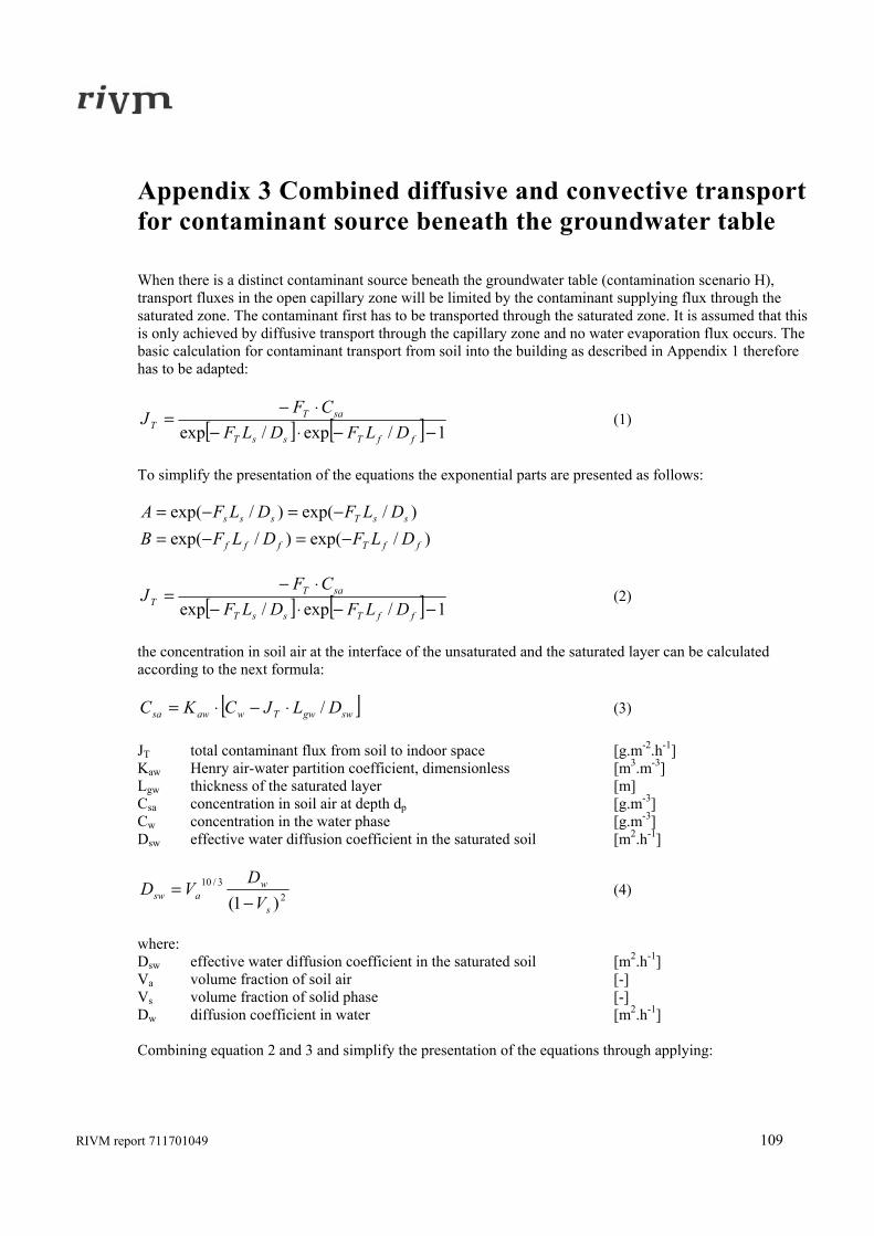
RIVM report 711701049 109
Appendix 3 Combined diffusive and convective transport for contaminant source beneath the groundwater table When there is a distinct contaminant source beneath the groundwater table (contamination scenario H), transport fluxes in the open capillary zone will be limited by the contaminant supplying flux through the saturated zone. The contaminant first has to be transported through the saturated zone. It is assumed that this is only achieved by diffusive transport through the capillary zone and no water evaporation flux occurs. The basic calculation for contaminant transport from soil into the building as described in Appendix 1 therefore has to be adapted:
[ ] [ ] 1/exp/exp −−⋅−⋅−
=ffTssT
saTT DLFDLF
CFJ (1)
To simplify the presentation of the equations the exponential parts are presented as follows:
)/exp()/exp()/exp()/exp(
ffTfff
ssTsss
DLFDLFBDLFDLFA
−=−=−=−=
[ ] [ ] 1/exp/exp −−⋅−⋅−
=ffTssT
saTT DLFDLF
CFJ (2)
the concentration in soil air at the interface of the unsaturated and the saturated layer can be calculated according to the next formula:
[ ]swgwTwawsa DLJCKC /⋅−⋅= (3) JT total contaminant flux from soil to indoor space [g.m-2.h-1] Kaw Henry air-water partition coefficient, dimensionless [m3.m-3] Lgw thickness of the saturated layer [m] Csa concentration in soil air at depth dp [g.m-3] Cw concentration in the water phase [g.m-3] Dsw effective water diffusion coefficient in the saturated soil [m2.h-1]
23/10
)1( s
wasw V
DVD
−= (4)
where: Dsw effective water diffusion coefficient in the saturated soil [m2.h-1] Va volume fraction of soil air [-] Vs volume fraction of solid phase [-] Dw diffusion coefficient in water [m2.h-1] Combining equation 2 and 3 and simplify the presentation of the equations through applying:
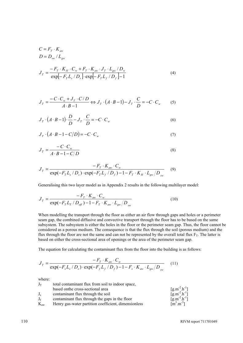
110 RIVM report 711701049
gwsw
awT
LDDKFC/=
⋅=
[ ] [ ] 1/exp/exp/−−⋅−
⋅⋅⋅+⋅⋅−=
ffTssT
wgwTawTwHTT DLFDLF
DLJKFCKFJ (4)
( ) wTTTw
T CCDCJBAJ
BADCJCC
J ⋅−=⋅−−⋅⋅⇔−⋅
⋅+⋅−= 1
1/
(5)
( ) wTT CCDCJ
DDBAJ ⋅−=⋅−⋅−⋅⋅ 1 (6)
( ) wT CCDCBAJ ⋅−=−−⋅⋅ 1 (7)
DCBACC
J wT −−⋅
⋅−=
1 (8)
swgwHTffTssT
wawTT DLKFDLFDLF
CKFJ
⋅⋅−−−⋅−⋅⋅−
=1)/exp()/exp(
(9)
Generalising this two layer model as in Appendix 2 results in the following multilayer model:
swgwawTeffTT
wawTT DLKFDLF
CKFJ
⋅⋅−−−⋅⋅−
=1)/exp(
(10)
When modelling the transport through the floor as either an air flow through gaps and holes or a perimeter seam gap, the combined diffusive and convective transport through the floor has to be based on the same subsystem. The subsystem is either the holes in the floor or the perimeter seam gap. Thus, the floor cannot be considered as a porous medium. The consequence is that the flux through the soil (porous medium) and the flux through the floor are not the same and can not be represented by the overall total flux FT. The latter is based on either the cross-sectional area of openings or the area of the perimeter seam gap. The equation for calculating the contaminant flux from the floor into the building is as follows:
swgwawsfffsss
wawTT DLKFDLFDLF
CKFJ
⋅⋅−−−⋅−⋅⋅−
=1)/exp()/exp(
(11)
where: JT total contaminant flux from soil to indoor space,
based onthe cross-sectional area [g.m-2.h-1] Js contaminant flux through the soil [g.m-2.h-1] Jf contaminant flux through the gaps in the floor [g.m-2.h-1] Kaw Henry gas-water partition coefficient, dimensionless [m3.m-3]
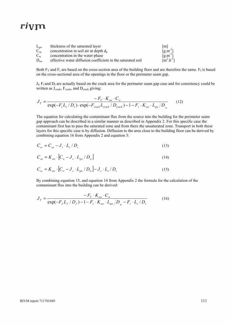
RIVM report 711701049 111
Lgw thickness of the saturated layer [m] Csa concentration in soil air at depth dp [g.m-3] Cw concentration in the water phase [g.m-3] Dsw effective water diffusion coefficient in the saturated soil [m2.h-1] Both FT and Fs are based on the cross-section area of the building floor and are therefore the same. Ff is based on the cross-sectional area of the openings in the floor or the perimeter seam gap. Jf, Ff and Df are actually based on the crack area for the perimeter seam gap case and for consistency could be written as Jcrack, Fcrack, and Dcrack giving:
wgwawscrackcrackcracksss
wawTT DLKFDLFDLF
CKFJ
⋅⋅−−−⋅−⋅⋅−
=1)/exp()/exp(
(12)
The equation for calculating the contaminant flux from the source into the building for the perimeter seam gap approach can be described in a similar manner as described in Appendix 2. For this specific case the contaminant first has to pass the saturated zone and from there the unsaturated zone. Transport in both these layers for this specific case is by diffusion. Diffusion to the area close to the building floor can be derived by combining equation 16 from Appendix 2 and equation 3:
ssssasc DLJCC /⋅−= (13)
[ ]wgwswawsa DLJCKC /⋅−⋅= (14)
[ ] ssswgwswawsc DLJDLJCKC // ⋅−⋅−⋅= (15) By combining equation 15, and equation 14 from Appendix 2 the formula for the calculation of the contaminant flux into the building can be derived:
ssswgwawsfff
wawTT DLFDLKFDLF
CKFJ
/1)/exp( ⋅−⋅⋅−−−⋅⋅−
= (16)
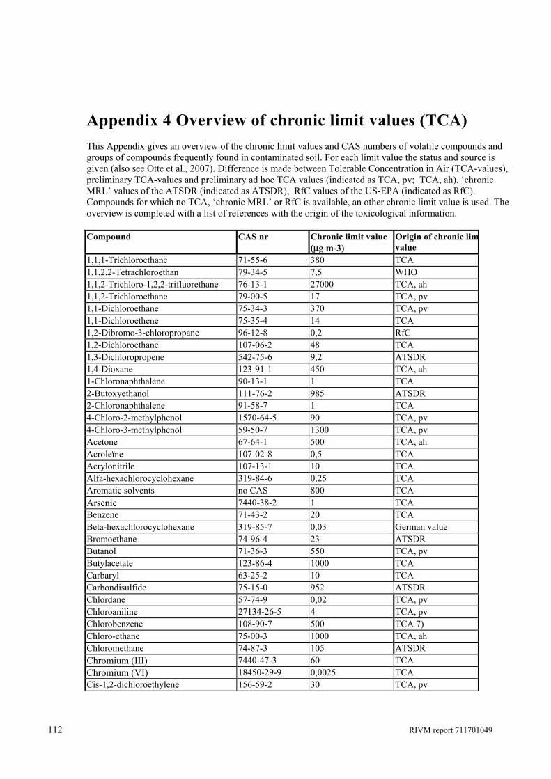
112 RIVM report 711701049
Appendix 4 Overview of chronic limit values (TCA) This Appendix gives an overview of the chronic limit values and CAS numbers of volatile compounds and groups of compounds frequently found in contaminated soil. For each limit value the status and source is given (also see Otte et al., 2007). Difference is made between Tolerable Concentration in Air (TCA-values), preliminary TCA-values and preliminary ad hoc TCA values (indicated as TCA, pv; TCA, ah), ‘chronic MRL’ values of the ATSDR (indicated as ATSDR), RfC values of the US-EPA (indicated as RfC). Compounds for which no TCA, ‘chronic MRL’ or RfC is available, an other chronic limit value is used. The overview is completed with a list of references with the origin of the toxicological information. Compound CAS nr Chronic limit value
(μg m-3) Origin of chronic limvalue
1,1,1-Trichloroethane 71-55-6 380 TCA 1,1,2,2-Tetrachloroethan 79-34-5 7,5 WHO 1,1,2-Trichloro-1,2,2-trifluorethane 76-13-1 27000 TCA, ah 1,1,2-Trichloroethane 79-00-5 17 TCA, pv 1,1-Dichloroethane 75-34-3 370 TCA, pv 1,1-Dichloroethene 75-35-4 14 TCA 1,2-Dibromo-3-chloropropane 96-12-8 0,2 RfC 1,2-Dichloroethane 107-06-2 48 TCA 1,3-Dichloropropene 542-75-6 9,2 ATSDR 1,4-Dioxane 123-91-1 450 TCA, ah 1-Chloronaphthalene 90-13-1 1 TCA 2-Butoxyethanol 111-76-2 985 ATSDR 2-Chloronaphthalene 91-58-7 1 TCA 4-Chloro-2-methylphenol 1570-64-5 90 TCA, pv 4-Chloro-3-methylphenol 59-50-7 1300 TCA, pv Acetone 67-64-1 500 TCA, ah Acroleïne 107-02-8 0,5 TCA Acrylonitrile 107-13-1 10 TCA Alfa-hexachlorocyclohexane 319-84-6 0,25 TCA Aromatic solvents no CAS 800 TCA Arsenic 7440-38-2 1 TCA Benzene 71-43-2 20 TCA Beta-hexachlorocyclohexane 319-85-7 0,03 German value Bromoethane 74-96-4 23 ATSDR Butanol 71-36-3 550 TCA, pv Butylacetate 123-86-4 1000 TCA Carbaryl 63-25-2 10 TCA Carbondisulfide 75-15-0 952 ATSDR Chlordane 57-74-9 0,02 TCA, pv Chloroaniline 27134-26-5 4 TCA, pv Chlorobenzene 108-90-7 500 TCA 7) Chloro-ethane 75-00-3 1000 TCA, ah Chloromethane 74-87-3 105 ATSDR Chromium (III) 7440-47-3 60 TCA Chromium (VI) 18450-29-9 0,0025 TCA Cis-1,2-dichloroethylene 156-59-2 30 TCA, pv
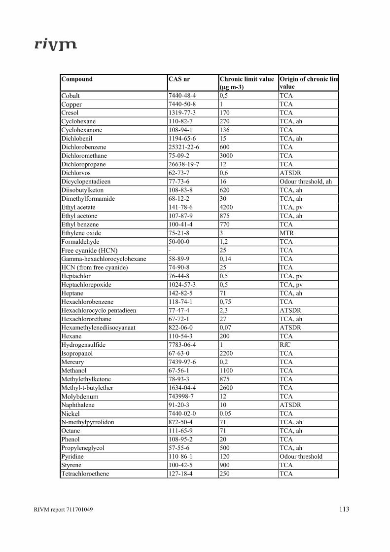
RIVM report 711701049 113
Compound CAS nr Chronic limit value (μg m-3)
Origin of chronic limvalue
Cobalt 7440-48-4 0,5 TCA Copper 7440-50-8 1 TCA Cresol 1319-77-3 170 TCA Cyclohexane 110-82-7 270 TCA, ah Cyclohexanone 108-94-1 136 TCA Dichlobenil 1194-65-6 15 TCA, ah Dichlorobenzene 25321-22-6 600 TCA Dichloromethane 75-09-2 3000 TCA Dichloropropane 26638-19-7 12 TCA Dichlorvos 62-73-7 0,6 ATSDR Dicyclopentadieen 77-73-6 16 Odour threshold, ah Diisobutylketon 108-83-8 620 TCA, ah Dimethylformamide 68-12-2 30 TCA, ah Ethyl acetate 141-78-6 4200 TCA, pv Ethyl acetone 107-87-9 875 TCA, ah Ethyl benzene 100-41-4 770 TCA Ethylene oxide 75-21-8 3 MTR Formaldehyde 50-00-0 1,2 TCA Free cyanide (HCN) - 25 TCA Gamma-hexachlorocyclohexane 58-89-9 0,14 TCA HCN (from free cyanide) 74-90-8 25 TCA Heptachlor 76-44-8 0,5 TCA, pv Heptachlorepoxide 1024-57-3 0,5 TCA, pv Heptane 142-82-5 71 TCA, ah Hexachlorobenzene 118-74-1 0,75 TCA Hexachlorocyclo pentadieen 77-47-4 2,3 ATSDR Hexachlororethane 67-72-1 27 TCA, ah Hexamethylenediisocyanaat 822-06-0 0,07 ATSDR Hexane 110-54-3 200 TCA Hydrogensulfide 7783-06-4 1 RfC Isopropanol 67-63-0 2200 TCA Mercury 7439-97-6 0,2 TCA Methanol 67-56-1 1100 TCA Methylethylketone 78-93-3 875 TCA Methyl-t-butylether 1634-04-4 2600 TCA Molybdenum 743998-7 12 TCA Naphthalene 91-20-3 10 ATSDR Nickel 7440-02-0 0.05 TCA N-methylpyrrolidon 872-50-4 71 TCA, ah Octane 111-65-9 71 TCA, ah Phenol 108-95-2 20 TCA Propyleneglycol 57-55-6 500 TCA, ah Pyridine 110-86-1 120 Odour threshold Styrene 100-42-5 900 TCA Tetrachloroethene 127-18-4 250 TCA
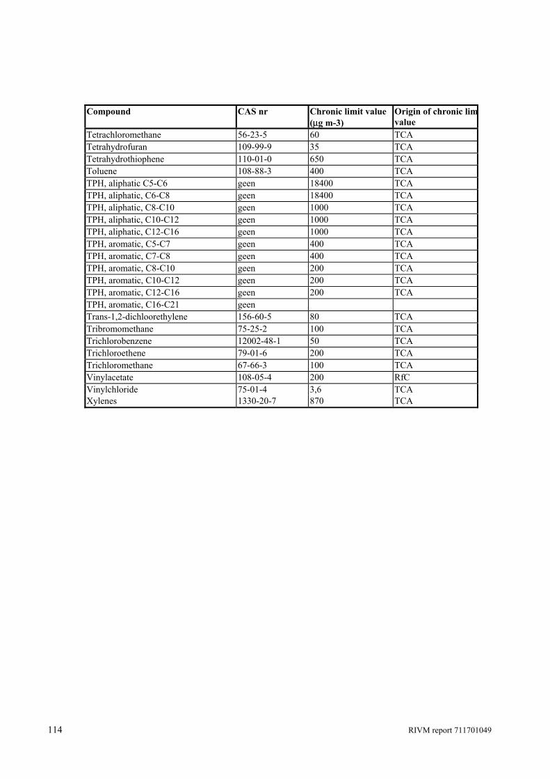
114 RIVM report 711701049
Compound CAS nr Chronic limit value (μg m-3)
Origin of chronic limvalue
Tetrachloromethane 56-23-5 60 TCA Tetrahydrofuran 109-99-9 35 TCA Tetrahydrothiophene 110-01-0 650 TCA Toluene 108-88-3 400 TCA TPH, aliphatic C5-C6 geen 18400 TCA TPH, aliphatic, C6-C8 geen 18400 TCA TPH, aliphatic, C8-C10 geen 1000 TCA TPH, aliphatic, C10-C12 geen 1000 TCA TPH, aliphatic, C12-C16 geen 1000 TCA TPH, aromatic, C5-C7 geen 400 TCA TPH, aromatic, C7-C8 geen 400 TCA TPH, aromatic, C8-C10 geen 200 TCA TPH, aromatic, C10-C12 geen 200 TCA TPH, aromatic, C12-C16 geen 200 TCA TPH, aromatic, C16-C21 geen Trans-1,2-dichloorethylene 156-60-5 80 TCA Tribromomethane 75-25-2 100 TCA Trichlorobenzene 12002-48-1 50 TCA Trichloroethene 79-01-6 200 TCA Trichloromethane 67-66-3 100 TCA Vinylacetate 108-05-4 200 RfC Vinylchloride 75-01-4 3,6 TCA Xylenes 1330-20-7 870 TCA
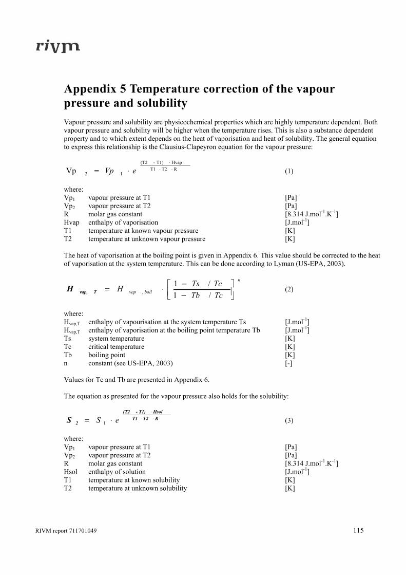
RIVM report 711701049 115
Appendix 5 Temperature correction of the vapour pressure and solubility Vapour pressure and solubility are physicochemical properties which are highly temperature dependent. Both vapour pressure and solubility will be higher when the temperature rises. This is also a substance dependent property and to which extent depends on the heat of vaporisation and heat of solubility. The general equation to express this relationship is the Clausius-Clapeyron equation for the vapour pressure:
RT2T1HvapT1)-(T2
12Vp ⋅⋅⋅
⋅= eVp (1) where: Vp1 vapour pressure at T1 [Pa] Vp2 vapour pressure at T2 [Pa] R molar gas constant [8.314 J.mol-1.K-1] Hvap enthalpy of vaporisation [J.mol-1] T1 temperature at known vapour pressure [K] T2 temperature at unknown vapour pressure [K] The heat of vaporisation at the boiling point is given in Appendix 6. This value should be corrected to the heat of vaporisation at the system temperature. This can be done according to Lyman (US-EPA, 2003).
n
boilvap TcTbTcTsH ⎥⎦
⎤⎢⎣⎡
−−⋅=
/1/1
,Tvap,H (2)
where: Hvap,T enthalpy of vapourisation at the system temperature Ts [J.mol-1] Hvap,T enthalpy of vaporisation at the boiling point temperature Tb [J.mol-1] Ts system temperature [K] Tc critical temperature [K] Tb boiling point [K] n constant (see US-EPA, 2003) [-] Values for Tc and Tb are presented in Appendix 6. The equation as presented for the vapour pressure also holds for the solubility:
RT2T1HsolT1)-(T2
2S ⋅⋅⋅
⋅= eS 1 (3) where: Vp1 vapour pressure at T1 [Pa] Vp2 vapour pressure at T2 [Pa] R molar gas constant [8.314 J.mol-1.K-1] Hsol enthalpy of solution [J.mol-1] T1 temperature at known solubility [K] T2 temperature at unknown solubility [K]
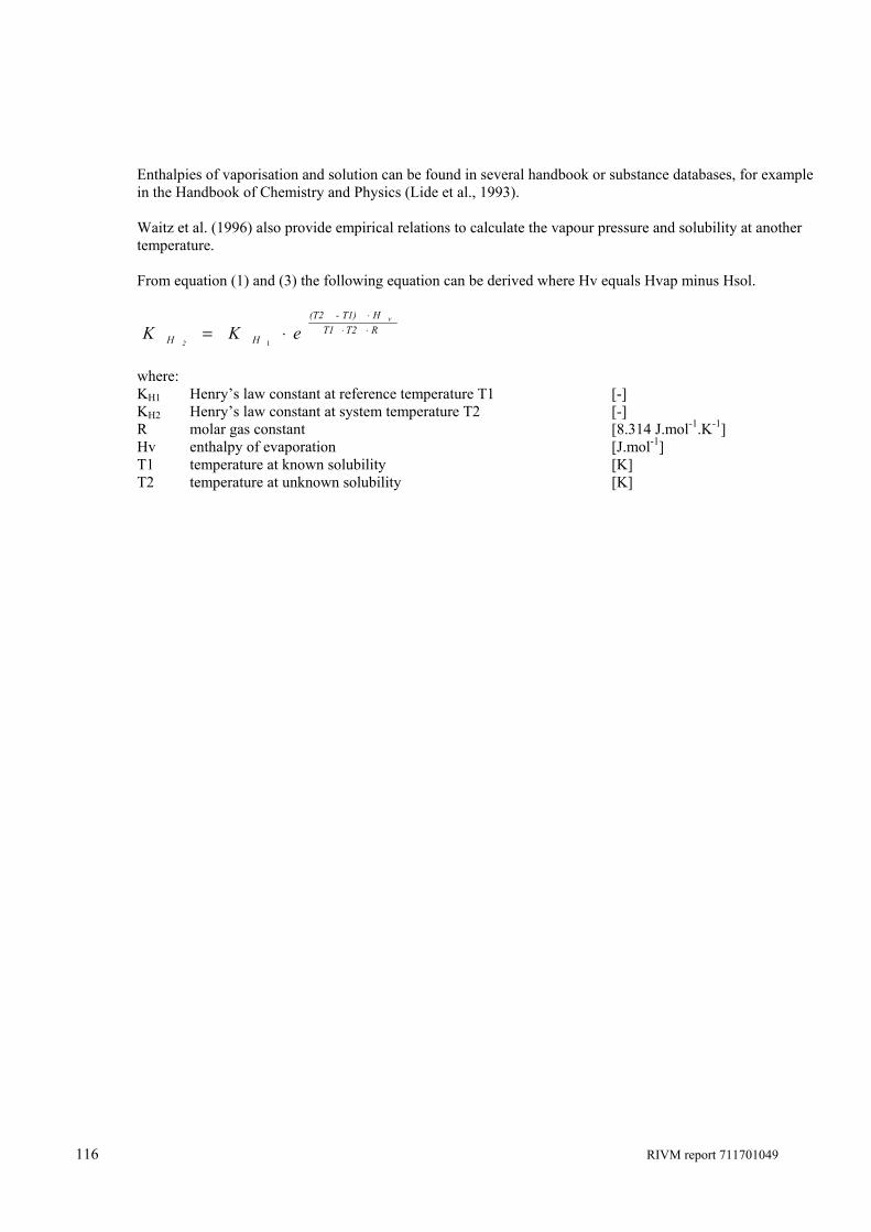
116 RIVM report 711701049
Enthalpies of vaporisation and solution can be found in several handbook or substance databases, for example in the Handbook of Chemistry and Physics (Lide et al., 1993). Waitz et al. (1996) also provide empirical relations to calculate the vapour pressure and solubility at another temperature. From equation (1) and (3) the following equation can be derived where Hv equals Hvap minus Hsol.
RT2T1HT1)-(T2
HH
v
2eKK ⋅⋅
⋅
⋅=1
where: KH1 Henry’s law constant at reference temperature T1 [-] KH2 Henry’s law constant at system temperature T2 [-] R molar gas constant [8.314 J.mol-1.K-1] Hv enthalpy of evaporation [J.mol-1] T1 temperature at known solubility [K] T2 temperature at unknown solubility [K]
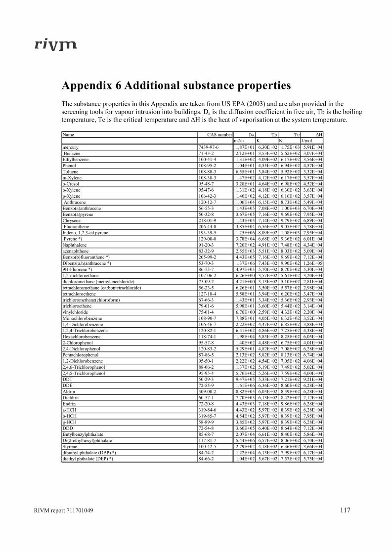
RIVM report 711701049 117
Appendix 6 Additional substance properties The substance properties in this Appendix are taken from US EPA (2003) and are also provided in the screening tools for vapour intrusion into buildings. Da is the diffusion coefficient in free air, Tb is the boiling temperature, Tc is the critical temperature and ΔH is the heat of vaporisation at the system temperature. Name CAS number Da Tb Tc ΔH
m2/h K K J/molmercury 7439-97-6 1,87E+01 6,30E+02 1,75E+03 5,91E+04 Benzene 71-43-2 2,12E+01 3,53E+02 5,62E+02 3,07E+04Ethylbenzene 100-41-4 1,31E+02 4,09E+02 6,17E+02 3,56E+04Phenol 108-95-2 1,04E+01 4,55E+02 6,94E+02 4,57E+04Toluene 108-88-3 6,55E+01 3,84E+02 5,92E+02 3,32E+04m-Xylene 108-38-3 1,47E+02 4,12E+02 6,17E+02 3,57E+04o-Cresol 95-48-7 3,28E+01 4,64E+02 6,98E+02 4,52E+04o-Xylene 95-47-6 1,31E+02 4,18E+02 6,30E+02 3,63E+04p-Xylene 106-42-3 1,40E+02 4,12E+02 6,16E+02 3,57E+04 Anthracene 120-12-7 1,06E+04 6,15E+02 8,73E+02 5,49E+04Benzo(a)anthracene 56-55-3 1,43E+05 7,08E+02 1,00E+03 6,70E+04Benzo(a)pyrene 50-32-8 3,67E+05 7,16E+02 9,69E+02 7,95E+04Chrysene 218-01-9 1,43E+05 7,14E+02 9,79E+02 6,89E+04 Fluoranthene 206-44-0 3,85E+04 6,56E+02 9,05E+02 5,78E+04Indeno, 1,2,3-cd pyrene 193-39-5 1,25E+06 8,09E+02 1,08E+03 7,95E+04 Pyrene *) 129-00-0 3,78E+04 6,68E+02 9,36E+02 6,01E+04Naphthalene 91-20-3 7,20E+02 4,91E+02 7,48E+02 4,34E+04acenaphthene 83-32-9 2,55E+03 5,51E+02 8,03E+02 5,09E+04Benzo(b)fluoranthene *) 205-99-2 4,43E+05 7,16E+02 9,69E+02 7,12E+04Dibenz(a,h)anthracene *) 53-70-3 1,37E+06 7,43E+02 9,90E+02 1,26E+059H-Fluorene *) 86-73-7 4,97E+03 5,70E+02 8,70E+02 5,30E+041,2-dichloroethane 107-06-2 6,26E+00 3,57E+02 5,61E+02 3,20E+04dichloromethane (methylenechloride) 75-09-2 4,21E+00 3,13E+02 5,10E+02 2,81E+04tetrachloromethane (carbontetrachloride) 56-23-5 6,26E+01 3,50E+02 5,57E+02 2,98E+04tetrachloroethene 127-18-4 5,58E+01 3,94E+02 6,20E+02 3,47E+04trichloromethane(chloroform) 67-66-3 1,43E+01 3,34E+02 5,36E+02 2,93E+04trichloroethene 79-01-6 5,98E+01 3,60E+02 5,44E+02 3,14E+04vinylchloride 75-01-4 6,70E+00 2,59E+02 4,32E+02 2,20E+04Monochlorobenzene 108-90-7 7,88E+01 4,05E+02 6,32E+02 3,52E+041,4-Dichlorobenzene 106-46-7 2,22E+02 4,47E+02 6,85E+02 3,88E+041,2,4-Trichlorobenzene 120-82-1 6,41E+02 4,86E+02 7,25E+02 4,38E+04Hexachlorobenzene 118-74-1 1,98E+04 5,83E+02 8,25E+02 6,05E+042-Chlorophenol 95-57-8 1,40E+02 4,48E+02 6,75E+02 4,01E+042,4-Dichlorophenol 120-83-2 5,29E+01 4,82E+02 7,08E+02 6,28E+04Pentachlorophenol 87-86-5 2,13E+02 5,82E+02 8,13E+02 6,74E+041,2-Dichlorobenzene 95-50-1 2,22E+02 4,54E+02 7,05E+02 4,06E+042,4,6-Trichlorophenol 88-06-2 1,37E+02 5,19E+02 7,49E+02 5,02E+042,4,5-Trichlorophenol 95-95-4 5,76E+02 5,26E+02 7,59E+02 4,60E+04DDT 50-29-3 9,47E+05 5,33E+02 7,21E+02 9,21E+04DDE 72-55-9 1,61E+06 6,36E+02 8,60E+02 6,28E+04Aldrin 309-00-2 8,82E+05 6,03E+02 8,39E+02 6,28E+04Dieldrin 60-57-1 7,70E+03 6,13E+02 8,42E+02 7,12E+04Endrin 72-20-8 4,43E+03 7,18E+02 9,86E+02 6,28E+04a-HCH 319-84-6 4,43E+02 5,97E+02 8,39E+02 6,28E+04b-HCH 319-85-7 4,54E+02 5,97E+02 8,39E+02 7,95E+04g-HCH 58-89-9 3,85E+02 5,97E+02 8,39E+02 6,28E+04DDD 72-54-8 3,60E+05 6,40E+02 8,64E+02 7,12E+04Butylbenzylphthalate 85-68-7 2,07E+04 6,61E+02 8,40E+02 5,86E+04Di(2-ethylhexyl)phthalate 117-81-7 5,44E+06 6,57E+02 8,06E+02 6,70E+04Styrene 100-42-5 2,79E+02 4,18E+02 6,36E+02 3,66E+04dibuthyl phthalate (DBP) *) 84-74-2 1,22E+04 6,13E+02 7,99E+02 6,17E+04diethyl phthalate (DEP) *) 84-66-2 1,04E+02 5,67E+02 7,57E+02 5,75E+04
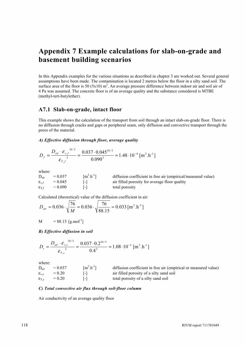
118 RIVM report 711701049
Appendix 7 Example calculations for slab-on-grade and basement building scenarios In this Appendix examples for the various situations as described in chapter 3 are worked out. Several general assumptions have been made. The contamination is located 2 metres below the floor in a silty sand soil. The surface area of the floor is 50 (5x10) m2. An average pressure difference between indoor air and soil air of 4 Pa was assumed. The concrete floor is of an average quality and the substance considered is MTBE (methyl-tert-butylether).
A7.1 Slab-on-grade, intact floor This example shows the calculation of the transport from soil through an intact slab-on-grade floor. There is no diffusion through cracks and gaps or peripheral seam, only diffusion and convective transport through the pores of the material. A) Effective diffusion through floor, average quality
].h[m 1048.1090.0
045.0037.0 1-242
3/10
2,
3/10, −⋅=⋅=
⋅=
fT
fvairf
DD
εε
where: Dair = 0.037 [m2.h-1] diffusion coefficient in free air (empirical/measured value) εv,f = 0.045 [-] air filled porosity for average floor quality εT,f = 0.090 [-] total porosity Calculated (theoretical) value of the diffusion coefficient in air:
].h[m033.015.88
76036.076036.0 1-2=⋅=⋅=M
Dair
M = 88.15 [g.mol-1] B) Effective diffusion in soil
].h[m1008.14.0
2.0037.0 1-232
3/10
2,
3/10, −⋅=⋅=
⋅=
sT
svairs
DD
εε
where: Dair = 0.037 [m2.h-1] diffusion coefficient in free air (empirical or measured value) εv,s = 0.20 [-] air filled porosity of a silty sand soil εT,s = 0.20 [-] total porosity of a silty sand soil C) Total convective air flux through soil-floor column Air conductivity of an average quality floor
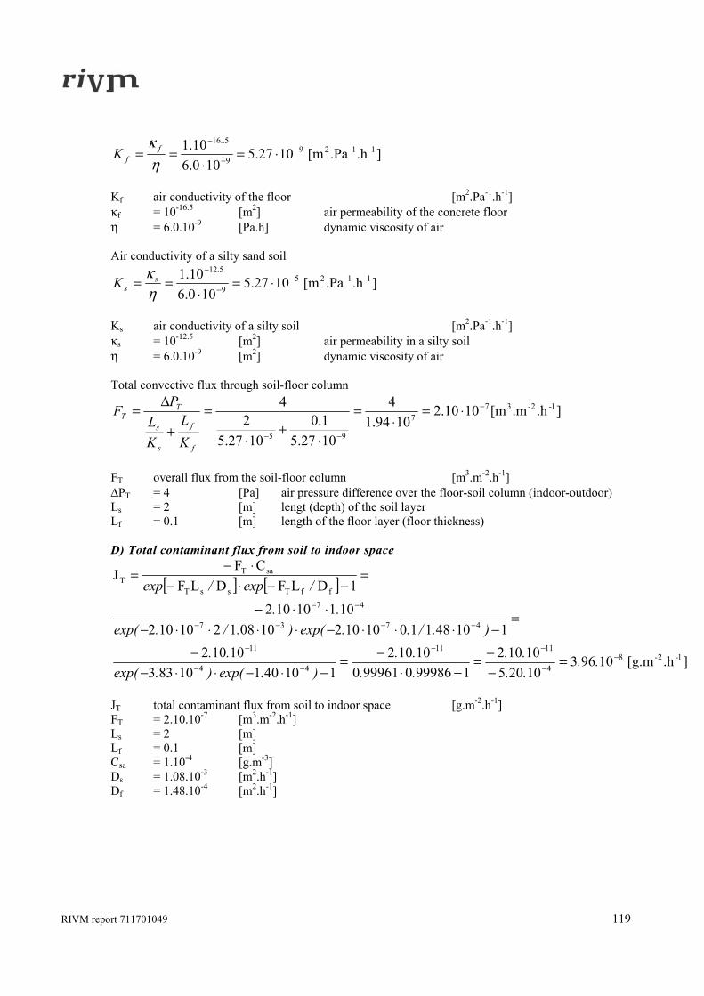
RIVM report 711701049 119
].h.Pa[m1027.5100.6
10.1 1-1-299
5..16−
−
−
⋅=⋅
==ηκ f
fK
Kf air conductivity of the floor [m2.Pa-1.h-1] κf = 10-16.5 [m2] air permeability of the concrete floor η = 6.0.10-9 [Pa.h] dynamic viscosity of air Air conductivity of a silty sand soil
].h.Pa[m1027.5100.6
10.1 1-1-259
5.12−
−
−
⋅=⋅
==ηκ s
sK
Ks air conductivity of a silty soil [m2.Pa-1.h-1] κs = 10-12.5 [m2] air permeability in a silty soil η = 6.0.10-9 [m2] dynamic viscosity of air Total convective flux through soil-floor column
].h.m[m1010.21094.1
4
1027.51.0
1027.52
4 1-2-377
95
−
−−
⋅=⋅
=
⋅+
⋅
=+
Δ=
f
f
s
s
TT
KL
KL
PF
FT overall flux from the soil-floor column [m3.m-2.h-1] ΔPT = 4 [Pa] air pressure difference over the floor-soil column (indoor-outdoor) Ls = 2 [m] lengt (depth) of the soil layer Lf = 0.1 [m] length of the floor layer (floor thickness) D) Total contaminant flux from soil to indoor space
[ ] [ ]
].h[g.m109631020510102
199986099961010102
1104011083310102
11048110101021008121010210110102
1DLFDLFCF
J
1-2-84
1111
44
11
4737
47ffTssT
saTT
−−
−−
−−
−
−−−−
−−
=−−=
−⋅−=
−⋅−⋅⋅−−
=−⋅⋅⋅−⋅⋅⋅⋅−
⋅⋅−
=−−⋅−
⋅−=
......
..
..).exp().exp(
..)./..exp()./.exp(
..
/exp/exp
JT total contaminant flux from soil to indoor space [g.m-2.h-1] FT = 2.10.10-7 [m3.m-2.h-1] Ls = 2 [m] Lf = 0.1 [m] Csa = 1.10-4 [g.m-3] Ds = 1.08.10-3 [m2.h-1] Df = 1.48.10-4 [m2.h-1]
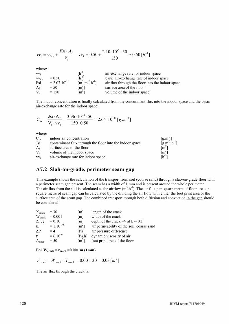
120 RIVM report 711701049
i
fbi,i V
AFsivvvv
⋅+= ][50.0
15050102.100.50vv 1
-7
i−≈⋅⋅+= h
where: vvi [h-1] air-exchange rate for indoor space vvi,b = 0.50 [h-1] basic air-exchange rate of indoor space Fsi = 2.07.10-11 [m3.m-2.h-1] air flux through the floor into the indoor space Af = 50 [m2] surface area of the floor Vi = 150 [m3] volume of the indoor space The indoor concentration is finally calculated from the contaminant flux into the indoor space and the basic air-exchange rate for the indoor space:
].[1064.250.0150
501096.3vvVAJsi
C 388
ii
fia
−−−
⋅=⋅
⋅⋅=⋅⋅
= mg
where: Cia indoor air concentration [g.m-3] Jsi contaminant flux through the floor into the indoor space [g.m-2.h-1] Af surface area of the floor [m2] Vi volume of the indoor space [m3] vvi air-exchange rate for indoor space [h-1]
A7.2 Slab-on-grade, perimeter seam gap This example shows the calculation of the transport from soil (course sand) through a slab-on-grade floor with a perimeter seam gap present. The seam has a width of 1 mm and is present around the whole perimeter. The air flux from the soil is calculated as the airflow (m3.h-1). The air flux per square metre of floor area or square metre of seam gap can be calculated by the dividing the air flow with either the foot print area or the surface area of the seam gap. The combined transport through both diffusion and convection in the gap should be considered. Xcrack = 30 [m] length of the crack Wcrack = 0.001 [m] width of the crack Zcrack = 0.10 [m] depth of the crack => at Lf= 0.1 κs = 1.10-10 [m2] air permeability of the soil, coarse sand ΔP = 4 [Pa] air pressure difference η = 6.10-9 [Pa.h] dynamic viscosity of air Afloor = 50 [m2] foot print area of the floor For Wcrack = rcrack =0.001 m (1mm)
][03.030001.0 2mXWA crackcrackcrack =⋅=⋅= The air flux through the crack is:
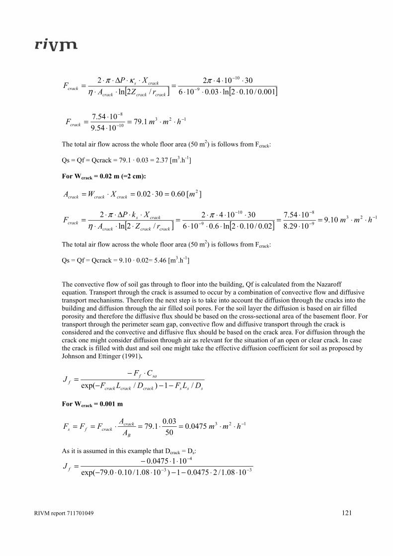
RIVM report 711701049 121
[ ] [ ]
12310
8
9
10
1.791054.91054.7
001.0/10.02ln03.0106301042
/2ln2
−−
−
−
−
⋅⋅=⋅⋅=
⋅⋅⋅⋅⋅⋅⋅=
⋅⋅⋅⋅Δ⋅⋅
=
hmmF
rZAXP
F
crack
crackcrackcrack
crackscrack
πη
κπ
The total air flow across the whole floor area (50 m2) is follows from Fcrack: Qs = Qf = Qcrack = 79.1 · 0.03 = 2.37 [m3.h-1] For Wcrack = 0.02 m (=2 cm):
][60.03002.0 2mXWA crackcrackcrack =⋅=⋅=
[ ] [ ]123
9
8
9
10
10.91029.81054.7
02.0/10.02ln6.0106301042
/2ln2 −
−
−
−
−
⋅⋅=⋅⋅=
⋅⋅⋅⋅⋅⋅⋅⋅=
⋅⋅⋅⋅⋅Δ⋅⋅
= hmmrZA
XkPF
crackcrackcrack
crackscrack
πη
π
The total air flow across the whole floor area (50 m2) is follows from Fcrack: Qs = Qf = Qcrack = 9.10 · 0.02= 5.46 [m3.h-1] The convective flow of soil gas through to floor into the building, Qf is calculated from the Nazaroff equation. Transport through the crack is assumed to occur by a combination of convective flow and diffusive transport mechanisms. Therefore the next step is to take into account the diffusion through the cracks into the building and diffusion through the air filled soil pores. For the soil layer the diffusion is based on air filled porosity and therefore the diffusive flux should be based on the cross-sectional area of the basement floor. For transport through the perimeter seam gap, convective flow and diffusive transport through the crack is considered and the convective and diffusive flux should be based on the crack area. For diffusion through the crack one might consider diffusion through air as relevant for the situation of an open or clear crack. In case the crack is filled with dust and soil one might take the effective diffusion coefficient for soil as proposed by Johnson and Ettinger (1991).
ssscrackcrackcrack
saff DLFDLF
CFJ
/1)/exp( −−−⋅−
=
For Wcrack = 0.001 m
1230475.05003.01.79 −⋅⋅=⋅=⋅== hmm
AA
FFFB
crackcrackfs
As it is assumed in this example that Dcrack = Ds:
33
4
1008.1/20475.01)1008.1/10.00.79exp(1010475.0
−−
−
⋅⋅−−⋅⋅−⋅⋅−=fJ
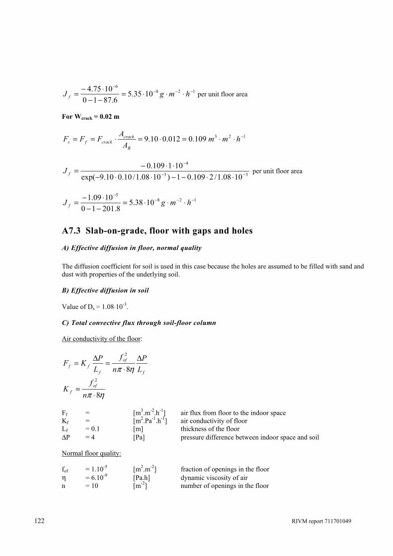
122 RIVM report 711701049
1286
1035.56.8710
1075.4 −−−−
⋅⋅⋅=−−
⋅−= hmgJ f per unit floor area
For Wcrack = 0.02 m
123109.0012.010.9 −⋅⋅=⋅=⋅== hmmA
AFFF
B
crackcrackfs
33
4
1008.1/2109.01)1008.1/10.010.9exp(101109.0
−−
−
⋅⋅−−⋅⋅−⋅⋅−=fJ per unit floor area
1285
1038.58.20110
1009.1 −−−−
⋅⋅⋅=−−
⋅−= hmgJ f
A7.3 Slab-on-grade, floor with gaps and holes A) Effective diffusion in floor, normal quality
The diffusion coefficient for soil is used in this case because the holes are assumed to be filled with sand and dust with properties of the underlying soil. B) Effective diffusion in soil Value of Ds = 1.08⋅10-3. C) Total convective flux through soil-floor column Air conductivity of the floor:
f
of
fff L
Pn
fL
PKF Δ⋅
=Δ=ηπ 8
2
ηπ 8
2
⋅=
nf
K off
Ff = [m3.m-2.h-1] air flux from floor to the indoor space Kf = [m2.Pa-1.h-1] air conductivity of floor Lf = 0.1 [m] thickness of the floor ΔP = 4 [Pa] pressure difference between indoor space and soil Normal floor quality: fof = 1.10-5 [m2.m-2] fraction of openings in the floor η = 6.10-9 [Pa.h] dynamic viscosity of air n = 10 [m-2] number of openings in the floor
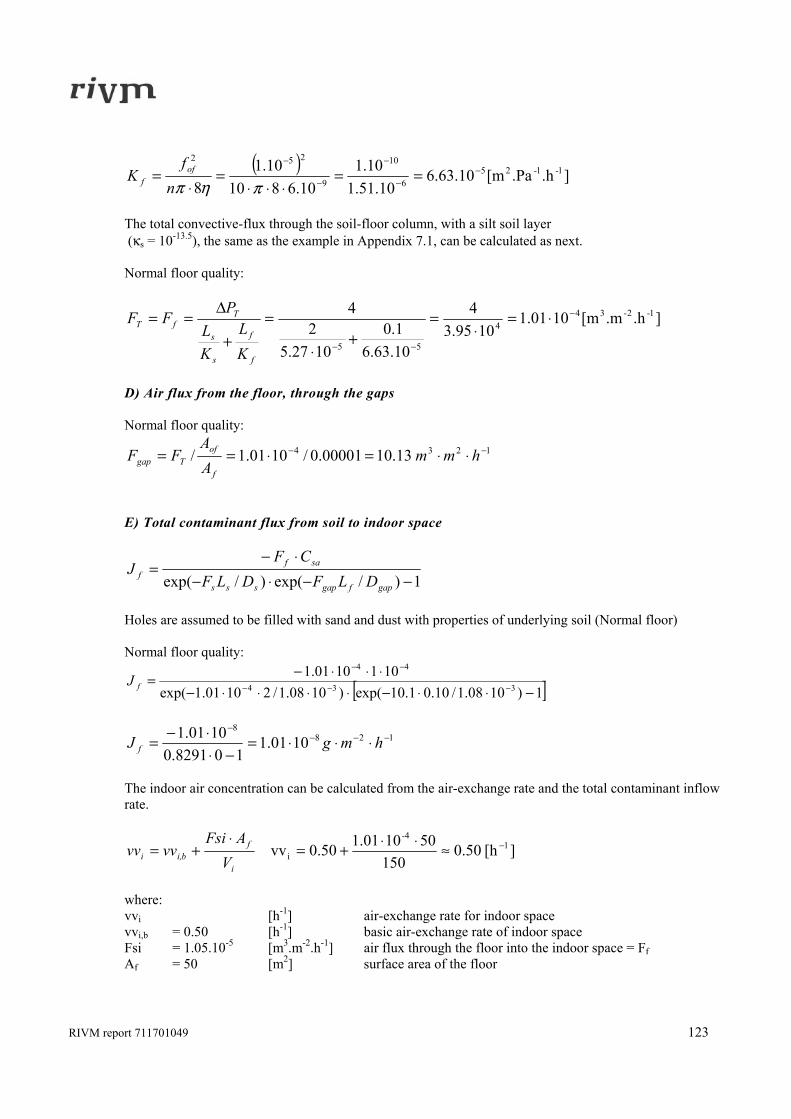
RIVM report 711701049 123
( ) ].h.Pa[m10.63.610.51.1
10.110.6810
10.18
1-1-256
10
9
252−
−
−
−
−
==⋅⋅⋅
=⋅
=πηπn
fK of
f
The total convective-flux through the soil-floor column, with a silt soil layer (κs = 10-13.5), the same as the example in Appendix 7.1, can be calculated as next. Normal floor quality:
].h.m[m1001.11095.3
4
10.63.61.0
1027.52
4 1-2-344
55
−
−−
⋅=⋅
=+
⋅
=+
Δ==
f
f
s
s
TfT
KL
KL
PFF
D) Air flux from the floor, through the gaps Normal floor quality:
1234 13.1000001.0/1001.1/ −− ⋅⋅=⋅== hmmAA
FFf
ofTgap
E) Total contaminant flux from soil to indoor space
1)/exp()/exp( −−⋅−⋅−
=gapfgapsss
saff DLFDLF
CFJ
Holes are assumed to be filled with sand and dust with properties of underlying soil (Normal floor) Normal floor quality:
[ ]1)1008.1/10.01.10exp()1008.1/21001.1exp(1011001.1
334
44
−⋅⋅−⋅⋅⋅⋅−⋅⋅⋅−= −−−
−−
fJ
1288
1001.1108291.0
1001.1 −−−−
⋅⋅⋅=−⋅
⋅−= hmgJ f
The indoor air concentration can be calculated from the air-exchange rate and the total contaminant inflow rate.
i
fbi,i V
AFsivvvv
⋅+= ][h0.50
15050101.010.50vv 1
-4
i−≈⋅⋅+=
where: vvi [h-1] air-exchange rate for indoor space vvi,b = 0.50 [h-1] basic air-exchange rate of indoor space Fsi = 1.05.10-5 [m3.m-2.h-1] air flux through the floor into the indoor space = Ff Af = 50 [m2] surface area of the floor
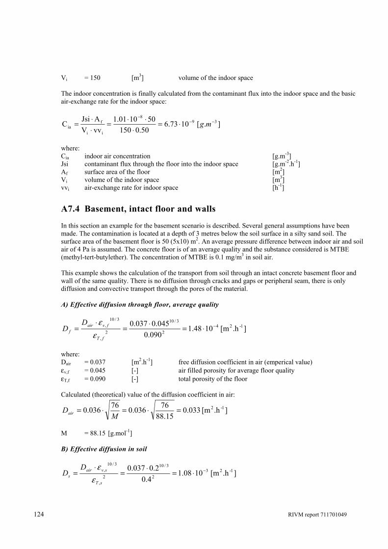
124 RIVM report 711701049
Vi = 150 [m3] volume of the indoor space The indoor concentration is finally calculated from the contaminant flux into the indoor space and the basic air-exchange rate for the indoor space:
].[1073.650.0150
501001.1vvVAJsi
C 398
ii
fia
−−−
⋅=⋅
⋅⋅=⋅⋅
= mg
where: Cia indoor air concentration [g.m-3] Jsi contaminant flux through the floor into the indoor space [g.m-2.h-1] Af surface area of the floor [m2] Vi volume of the indoor space [m3] vvi air-exchange rate for indoor space [h-1]
A7.4 Basement, intact floor and walls In this section an example for the basement scenario is described. Several general assumptions have been made. The contamination is located at a depth of 3 metres below the soil surface in a silty sand soil. The surface area of the basement floor is 50 (5x10) m2. An average pressure difference between indoor air and soil air of 4 Pa is assumed. The concrete floor is of an average quality and the substance considered is MTBE (methyl-tert-butylether). The concentration of MTBE is 0.1 mg/m3 in soil air. This example shows the calculation of the transport from soil through an intact concrete basement floor and wall of the same quality. There is no diffusion through cracks and gaps or peripheral seam, there is only diffusion and convective transport through the pores of the material. A) Effective diffusion through floor, average quality
].h[m 1048.1090.0
045.0037.0 1-242
3/10
2,
3/10, −⋅=⋅=
⋅=
fT
fvairf
DD
εε
where: Dair = 0.037 [m2.h-1] free diffusion coefficient in air (emperical value) εv,f = 0.045 [-] air filled porosity for average floor quality εT,f = 0.090 [-] total porosity of the floor Calculated (theoretical) value of the diffusion coefficient in air:
].h[m033.015.88
76036.076036.0 1-2=⋅=⋅=M
Dair
M = 88.15 [g.mol-1] B) Effective diffusion in soil
].h[m1008.14.0
2.0037.0 1-232
3/10
2,
3/10, −⋅=⋅=
⋅=
sT
svairs
DD
εε
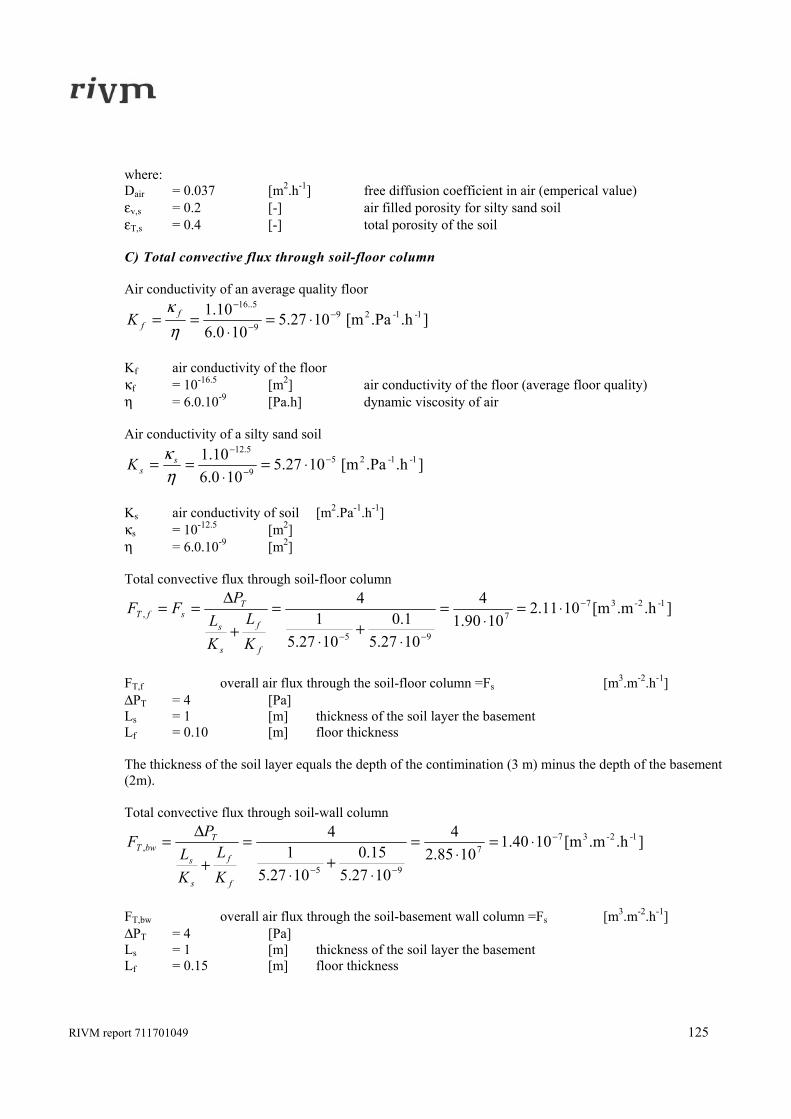
RIVM report 711701049 125
where: Dair = 0.037 [m2.h-1] free diffusion coefficient in air (emperical value) εv,s = 0.2 [-] air filled porosity for silty sand soil εT,s = 0.4 [-] total porosity of the soil C) Total convective flux through soil-floor column Air conductivity of an average quality floor
].h.Pa[m1027.5100.6
10.1 1-1-299
5..16−
−
−
⋅=⋅
==ηκ f
fK
Kf air conductivity of the floor κf = 10-16.5 [m2] air conductivity of the floor (average floor quality) η = 6.0.10-9 [Pa.h] dynamic viscosity of air Air conductivity of a silty sand soil
].h.Pa[m1027.5100.6
10.1 1-1-259
5.12−
−
−
⋅=⋅
==ηκ s
sK
Ks air conductivity of soil [m2.Pa-1.h-1] κs = 10-12.5 [m2] η = 6.0.10-9 [m2] Total convective flux through soil-floor column
].h.m[m1011.21090.1
4
1027.51.0
1027.51
4 1-2-377
95
,−
−−
⋅=⋅
=
⋅+
⋅
=+
Δ==
f
f
s
s
TsfT
KL
KL
PFF
FT,f overall air flux through the soil-floor column =Fs [m3.m-2.h-1] ΔPT = 4 [Pa] Ls = 1 [m] thickness of the soil layer the basement Lf = 0.10 [m] floor thickness The thickness of the soil layer equals the depth of the contimination (3 m) minus the depth of the basement (2m). Total convective flux through soil-wall column
].h.m[m1040.11085.2
4
1027.515.0
1027.51
4 1-2-377
95
,−
−−
⋅=⋅
=
⋅+
⋅
=+
Δ=
f
f
s
s
TbwT
KL
KL
PF
FT,bw overall air flux through the soil-basement wall column =Fs [m3.m-2.h-1] ΔPT = 4 [Pa] Ls = 1 [m] thickness of the soil layer the basement Lf = 0.15 [m] floor thickness
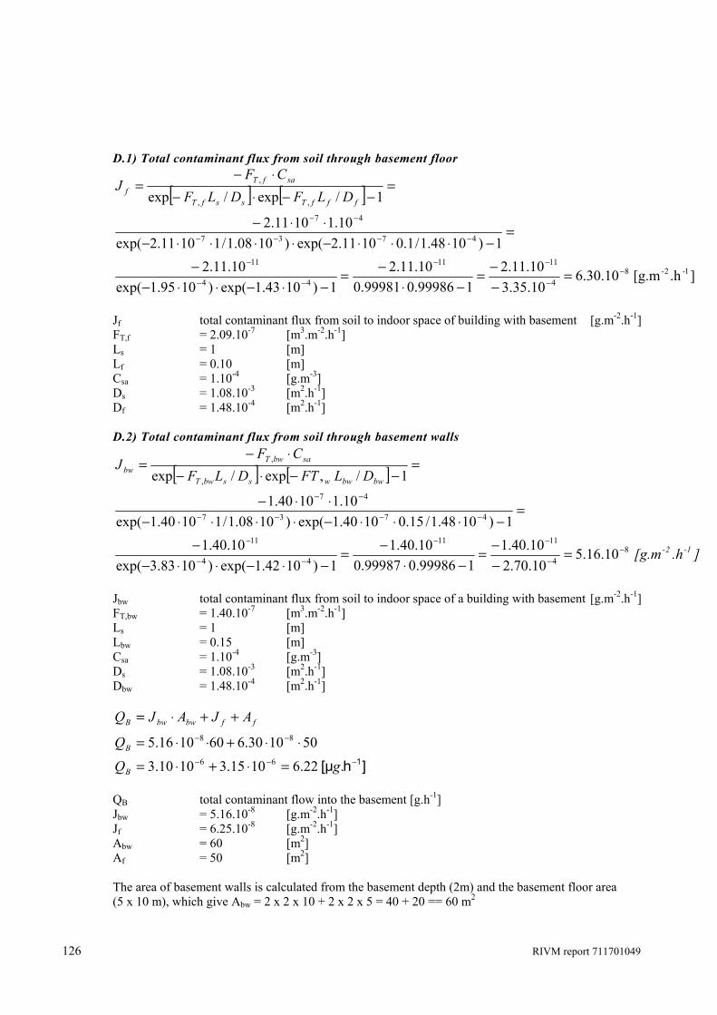
126 RIVM report 711701049
D.1) Total contaminant flux from soil through basement floor
[ ] [ ]
].h[g.m10.30.610.35.310.11.2
199986.099981.010.11.2
1)1043.1exp()1095.1exp(10.11.2
1)1048.1/1.01011.2exp()1008.1/11011.2exp(10.11011.2
1/exp/exp
1-2-84
1111
44
11
4737
47
,,
,
−−
−−
−−
−
−−−−
−−
=−−=
−⋅−=
−⋅−⋅⋅−−
=−⋅⋅⋅−⋅⋅⋅⋅−
⋅⋅−
=−−⋅−
⋅−=
fffTssfT
safTf DLFDLF
CFJ
Jf total contaminant flux from soil to indoor space of building with basement [g.m-2.h-1] FT,f = 2.09.10-7 [m3.m-2.h-1] Ls = 1 [m] Lf = 0.10 [m] Csa = 1.10-4 [g.m-3] Ds = 1.08.10-3 [m2.h-1] Df = 1.48.10-4 [m2.h-1] D.2) Total contaminant flux from soil through basement walls
[ ] [ ]
].h[g.m
DLFTDLFCF
J
1-2-
bwbwwssbwT
sabwTbw
84
1111
44
11
4737
47
,
,
10.16.510.70.210.40.1
199986.099987.010.40.1
1)1042.1exp()1083.3exp(10.40.1
1)1048.1/15.01040.1exp()1008.1/11040.1exp(10.11040.1
1/,exp/exp
−−
−−
−−
−
−−−−
−−
=−−=
−⋅−=
−⋅−⋅⋅−−
=−⋅⋅⋅−⋅⋅⋅⋅−
⋅⋅−
=−−⋅−
⋅−=
Jbw total contaminant flux from soil to indoor space of a building with basement [g.m-2.h-1] FT,bw = 1.40.10-7 [m3.m-2.h-1] Ls = 1 [m] Lbw = 0.15 [m] Csa = 1.10-4 [g.m-3] Ds = 1.08.10-3 [m2.h-1] Dbw = 1.48.10-4 [m2.h-1]
]h[μ 1−−−
−−
=⋅+⋅=
⋅⋅+⋅⋅=
++⋅=
.22.61015.31010.3
501030.6601016.566
88
gQ
Q
AJAJQ
B
B
ffbwbwB
QB total contaminant flow into the basement [g.h-1] Jbw = 5.16.10-8 [g.m-2.h-1] Jf = 6.25.10-8 [g.m-2.h-1] Abw = 60 [m2] Af = 50 [m2] The area of basement walls is calculated from the basement depth (2m) and the basement floor area (5 x 10 m), which give Abw = 2 x 2 x 10 + 2 x 2 x 5 = 40 + 20 == 60 m2
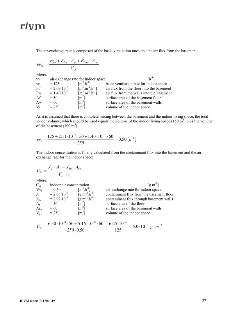
RIVM report 711701049 127
The air-exchange rate is composed of the basic ventilation rates and the air flux from the basement:
bi,
bwbwT,ffT,bi,bi, V
AFAFvrvv
⋅+⋅+=
where: vv air-exchange rate for indoor space [h-1] vr = 125 [m3.h-1] basic ventilation rate for indoor space Ff = 2.09.10-7 [m3.m-2.h-1] air flux from the floor into the basement Fw = 1.40.10-7 [m3.m-2.h-1] air flux from the walls into the basement Af = 50 [m2] surface area of the basement floor Aw = 60 [m2] surface area of the basement walls Vi = 250 [m3] volume of the indoor space As it is assumed that there is complete mixing between the basement and the indoor living space, the total indoor volume, which should be used equals the volume of the indoor living space (150 m3) plus the volume of the basement (100 m3).
][50.0601040.1501011.2125 177
−−−
=⋅⋅+⋅⋅+= h250
vvi
The indoor concentration is finally calculated from the contaminant flux into the basement and the air-exchange rate for the indoor space:
ii
bwbwffia vvV
AJAJC
⋅⋅+⋅
=
where: Cia indoor air concentration [g.m-3] Vvi = 0.50 [m3.h-1] air-exchange rate for indoor space Jf = 2.65.10-8 [g.m-2.h-1] contaminant flux from the basement floor Jbw = 2.92.10-8 [g.m-2.h-1] contaminant flux through basement walls Af = 50 [m2] surface area of the floor Abw = 60 [m2] surface area of the basement walls Vi = 250 [m3] volume of the indoor space
38688
100.5125
1025.650.0
601016.5501030.6 −−−−−
⋅⋅=⋅=⋅
⋅⋅+⋅⋅= mg250
Cia
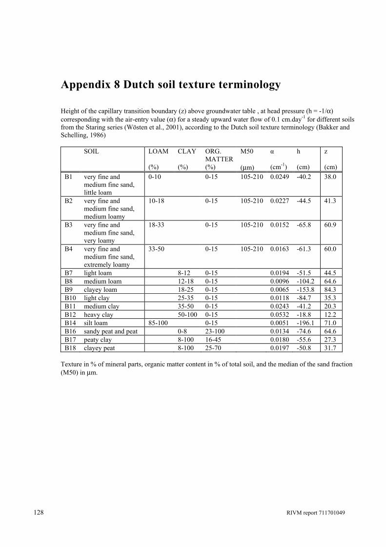
128 RIVM report 711701049
Appendix 8 Dutch soil texture terminology Height of the capillary transition boundary (z) above groundwater table , at head pressure (h = -1/α) corresponding with the air-entry value (α) for a steady upward water flow of 0.1 cm.day-1 for different soils from the Staring series (Wösten et al., 2001), according to the Dutch soil texture terminology (Bakker and Schelling, 1986)
SOIL LOAM CLAY ORG. MATTER
M50 α h z
(%) (%) (%) (μm) (cm-1) (cm) (cm) B1 very fine and
medium fine sand, little loam
0-10 0-15 105-210 0.0249 -40.2 38.0
B2 very fine and medium fine sand, medium loamy
10-18 0-15 105-210 0.0227 -44.5 41.3
B3 very fine and medium fine sand, very loamy
18-33 0-15 105-210 0.0152 -65.8 60.9
B4 very fine and medium fine sand, extremely loamy
33-50 0-15 105-210 0.0163 -61.3 60.0
B7 light loam 8-12 0-15 0.0194 -51.5 44.5 B8 medium loam 12-18 0-15 0.0096 -104.2 64.6 B9 clayey loam 18-25 0-15 0.0065 -153.8 84.3 B10 light clay 25-35 0-15 0.0118 -84.7 35.3 B11 medium clay 35-50 0-15 0.0243 -41.2 20.3 B12 heavy clay 50-100 0-15 0.0532 -18.8 12.2 B14 silt loam 85-100 0-15 0.0051 -196.1 71.0 B16 sandy peat and peat 0-8 23-100 0.0134 -74.6 64.6 B17 peaty clay 8-100 16-45 0.0180 -55.6 27.3 B18 clayey peat 8-100 25-70 0.0197 -50.8 31.7
Texture in % of mineral parts, organic matter content in % of total soil, and the median of the sand fraction (M50) in μm.
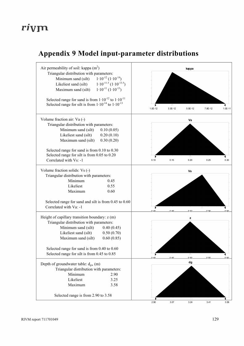
RIVM report 711701049 129
Appendix 9 Model input-parameter distributions
Air permeability of soil: kappa (m2) Triangular distribution with parameters: Minimum sand (silt) 1·10-12 (1·10-14) Likeliest sand (silt) 1·10-11.5 (1·10-13.5) Maximum sand (silt) 1·10-11 (1·10-13)
Selected range for sand is from 1·10-12 to 1·10-11
Selected range for silt is from 1·10-14 to 1·10-13
Volume fraction air: Va (-) Triangular distribution with parameters: Minimum sand (silt) 0.10 (0.05) Likeliest sand (silt) 0.20 (0.10) Maximum sand (silt) 0.30 (0.20)
Selected range for sand is from 0.10 to 0.30 Selected range for silt is from 0.05 to 0.20
Correlated with Vs: -1
Volume fraction solids: Vs (-) Triangular distribution with parameters: Minimum 0.45 Likeliest 0.55 Maximum 0.60 Selected range for sand and silt is from 0.45 to 0.60 Correlated with Va: -1
Height of capillary transition boundary: z (m) Triangular distribution with parameters: Minimum sand (silt) 0.40 (0.45) Likeliest sand (silt) 0.50 (0.70) Maximum sand (silt) 0.60 (0.85) Selected range for sand is from 0.40 to 0.60 Selected range for silt is from 0.45 to 0.85
Depth of groundwater table: dgw (m) Triangular distribution with parameters: Minimum 2.90 Likeliest 3.25 Maximum 3.58 Selected range is from 2.90 to 3.58
1.0E-12 3.3E-12 5.5E-12 7.8E-12 1.0E-11
kappa
0.10 0.15 0.20 0.25 0.30
Va
0.45 0.49 0.53 0.56 0.60
Vs
0.40 0.45 0.50 0.55 0.60
z
2.90 3.07 3.24 3.41 3.58
dg
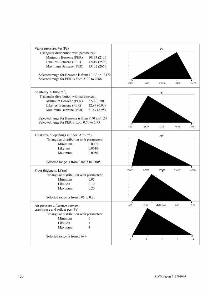
130 RIVM report 711701049
Vapor pressure: Vp (Pa) Triangular distribution with parameters: Minimum Benzene (PER) 10133 (2100) Likeliest Benzene (PER) 12419 (2500) Maximum Benzene (PER) 13172 (2666)
Selected range for Benzene is from 10133 to 13172Selected range for PER is from 2100 to 2666
Solubility: S (mol·m-3) Triangular distribution with parameters: Minimum Benzene (PER) 8.50 (0.70) Likeliest Benzene (PER) 22.97 (0.90) Maximum Benzene (PER) 61.67 (2.95)
Selected range for Benzene is from 8.50 to 61.67 Selected range for PER is from 0.70 to 2.95
Total area of openings in floor: Aof (m2) Triangular distribution with parameters: Minimum 0.0005 Likeliest 0.0010 Maximum 0.0050 Selected range is from 0.0005 to 0.005
Floor thickness: Lf (m) Triangular distribution with parameters: Minimum 0.05 Likeliest 0.10 Maximum 0.20 Selected range is from 0.05 to 0.20
Air pressure difference between crawlspace and soil: Δ pcs (Pa) Triangular distribution with parameters: Minimum 0 Likeliest 1 Maximum 4 Selected range is from 0 to 4
10133 10893 11653 12412 13172
Vp
8.50 21.79 35.09 48.38 61.67
S
0 1 2 3 4
delta pcs
0.0005 0.0016 0.0028 0.0039 0.0050
Aof
0.05 0.09 0.13 0.16 0.20
Lf
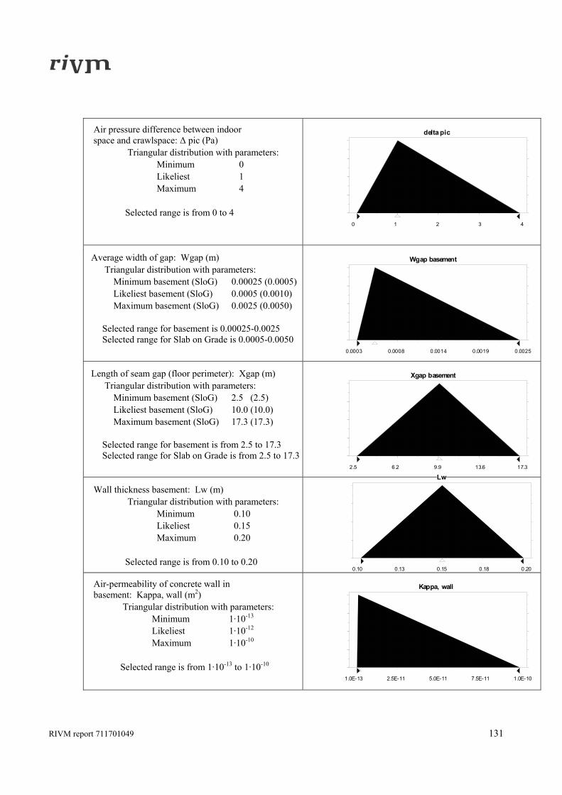
RIVM report 711701049 131
Air pressure difference between indoor space and crawlspace: Δ pic (Pa) Triangular distribution with parameters: Minimum 0 Likeliest 1 Maximum 4 Selected range is from 0 to 4
Average width of gap: Wgap (m) Triangular distribution with parameters: Minimum basement (SloG) 0.00025 (0.0005) Likeliest basement (SloG) 0.0005 (0.0010) Maximum basement (SloG) 0.0025 (0.0050)
Selected range for basement is 0.00025-0.0025 Selected range for Slab on Grade is 0.0005-0.0050
Length of seam gap (floor perimeter): Xgap (m) Triangular distribution with parameters: Minimum basement (SloG) 2.5 (2.5) Likeliest basement (SloG) 10.0 (10.0) Maximum basement (SloG) 17.3 (17.3)
Selected range for basement is from 2.5 to 17.3 Selected range for Slab on Grade is from 2.5 to 17.3
Wall thickness basement: Lw (m) Triangular distribution with parameters: Minimum 0.10 Likeliest 0.15 Maximum 0.20 Selected range is from 0.10 to 0.20
Air-permeability of concrete wall in basement: Kappa, wall (m2) Triangular distribution with parameters: Minimum 1·10-13 Likeliest 1·10-12 Maximum 1·10-10 Selected range is from 1·10-13 to 1·10-10
0 1 2 3 4
delta pic
0.0003 0.0008 0.0014 0.0019 0.0025
Wgap basement
2.5 6.2 9.9 13.6 17.3
Xgap basement
0.10 0.13 0.15 0.18 0.20
Lw
1.0E-13 2.5E-11 5.0E-11 7.5E-11 1.0E-10
Kappa, wall
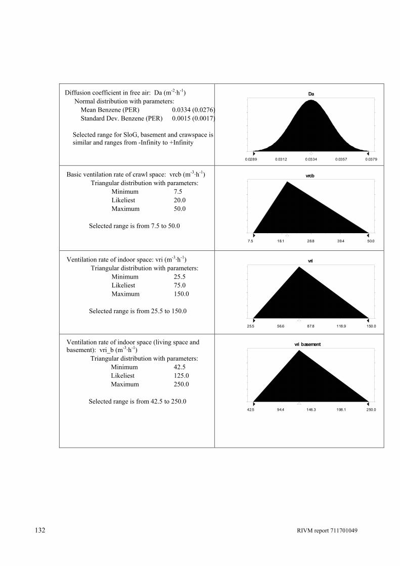
132 RIVM report 711701049
Diffusion coefficient in free air: Da (m-2·h-1) Normal distribution with parameters: Mean Benzene (PER) 0.0334 (0.0276) Standard Dev. Benzene (PER) 0.0015 (0.0017)
Selected range for SloG, basement and crawspace is similar and ranges from -Infinity to +Infinity
Basic ventilation rate of crawl space: vrcb (m-3·h-1) Triangular distribution with parameters: Minimum 7.5 Likeliest 20.0 Maximum 50.0 Selected range is from 7.5 to 50.0
Ventilation rate of indoor space: vri (m-3·h-1) Triangular distribution with parameters: Minimum 25.5 Likeliest 75.0 Maximum 150.0 Selected range is from 25.5 to 150.0
Ventilation rate of indoor space (living space and basement): vri_b (m-3·h-1) Triangular distribution with parameters: Minimum 42.5 Likeliest 125.0 Maximum 250.0 Selected range is from 42.5 to 250.0
0.0289 0.0312 0.0334 0.0357 0.0379
Da
7.5 18.1 28.8 39.4 50.0
vrcb
25.5 56.6 87.8 118.9 150.0
vri
42.5 94.4 146.3 198.1 250.0
vri basement
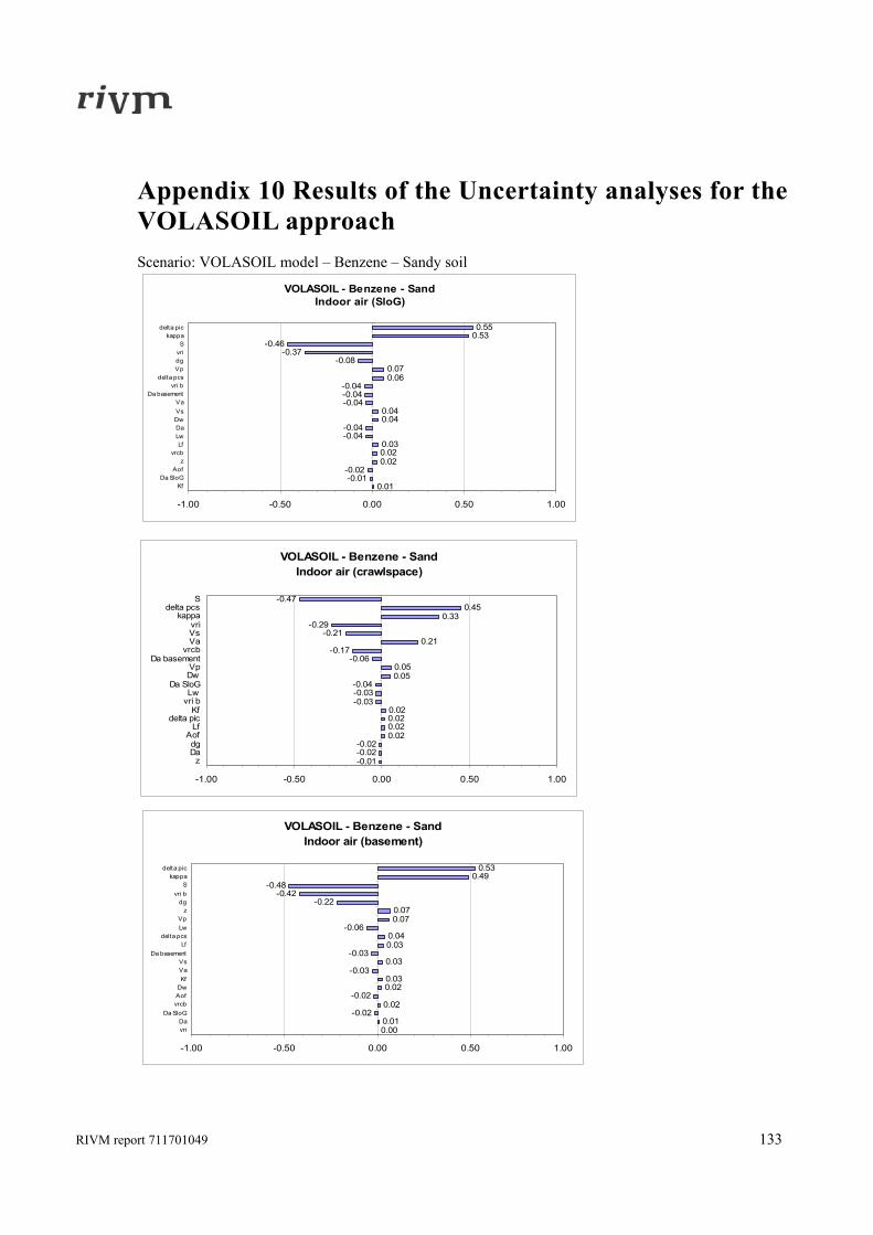
RIVM report 711701049 133
Appendix 10 Results of the Uncertainty analyses for the VOLASOIL approach Scenario: VOLASOIL model – Benzene – Sandy soil
VOLASOIL - Benzene - SandIndoor air (SloG)
0.01-0.01-0.02
0.020.020.03
-0.04-0.04
0.040.04
-0.04-0.04-0.04
0.060.07
-0.08-0.37
-0.460.530.55
-1.00 -0.50 0.00 0.50 1.00
KfDa SloG
Aofz
vrcbLf
LwDaDwVsVa
Da basementvri b
delta pcsVpdgvriS
kappadelta pic
VOLASOIL - Benzene - SandIndoor air (crawlspace)
-0.01-0.02-0.02
0.020.020.020.02
-0.03-0.03-0.04
0.050.05
-0.06-0.17
0.21-0.21
-0.290.33
0.45-0.47
-1.00 -0.50 0.00 0.50 1.00
zDadg
AofLf
delta picKf
vri bLw
Da SloGDwVp
Da basementvrcb
VaVsvri
kappadelta pcs
S
VOLASOIL - Benzene - SandIndoor air (basement)
0.000.01
-0.020.02
-0.020.020.03
-0.030.03
-0.030.030.04
-0.060.070.07
-0.22-0.42
-0.480.49
0.53
-1.00 -0.50 0.00 0.50 1.00
vriDa
Da SloGvrcbAofDwKfVaVs
Da basementLf
delta pcsLwVp
zdg
vri bS
kappadelta pic
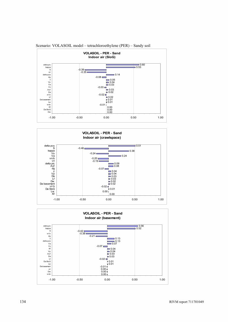
134 RIVM report 711701049
Scenario: VOLASOIL model – tetrachloroethylene (PER) – Sandy soil
VOLASOIL - PER - SandIndoor air (SloG)
0.000.000.00
-0.010.010.010.02
-0.020.020.03
-0.030.030.040.05
-0.080.14
-0.35-0.39
0.530.60
-1.00 -0.50 0.00 0.50 1.00
DwDa SloG
Kfvrcb
LwDa basement
Lfvri b
DaAofVsVaVp
zdg
delta pcsvriS
kappadelta pic
VOLASOIL - PER - SandIndoor air (crawlspace)
0.000.00
0.01-0.02
0.020.020.030.030.040.04
-0.070.080.09
-0.19-0.20
0.24-0.24
0.38-0.46
0.51
-1.00 -0.50 0.00 0.50 1.00
KfLw
Da SloGvri b
Da basementDw
LfDaVp
zdg
Aofdelta pic
vrivrcb
VaVs
kappaS
delta pcs
VOLASOIL - PER - SandIndoor air (basement)
0.000.000.00
-0.010.010.01
-0.020.030.030.040.04
-0.070.07
0.130.13
-0.21-0.38
-0.420.52
0.56
-1.00 -0.50 0.00 0.50 1.00
vrcbDwvri
Da basementLw
Da SloGLf
DaAofVpKfVsVa
delta pcsz
dgvri b
Skappa
delta pic
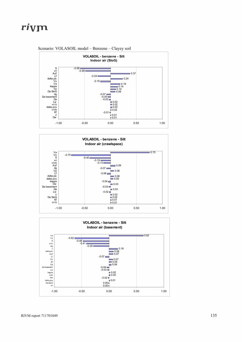
RIVM report 711701049 135
Scenario: VOLASOIL model – Benzene – Clayey soil
VOLASOIL - benzene - SiltIndoor air (SloG)
0.010.01
-0.010.020.020.020.02
-0.03-0.05
-0.070.090.10
0.140.19
-0.190.24
-0.240.37
-0.48-0.58
-1.00 -0.50 0.00 0.50 1.00
Dwz
Kfvrcb
delta pcsvri bLwDa
Da basementdg
Da SloGVp
kappaVaVs
delta picLf
AofvriS
VOLASOIL - benzene - SiltIndoor air (crawlspace)
0.010.010.020.02
-0.020.03
-0.030.03
-0.040.050.06
-0.060.06
-0.070.09
-0.13-0.19
-0.40-0.75
0.75
-1.00 -0.50 0.00 0.50 1.00
vri bKf
Da SloGz
LwDa
Da basementDw
kappadelta pcsdelta pic
LfVpdg
Aofvrcb
vriS
VsVa
VOLASOIL - benzene - SiltIndoor air (basement)
0.000.00
0.01-0.02
0.020.02
-0.03-0.04
0.040.050.07
-0.070.070.08
0.16-0.28
-0.41-0.48
-0.620.62
-1.00 -0.50 0.00 0.50 1.00
vriDa SloG
delta pcsDw
vrcbkappa
LwDa basement
DaKf
VpLf
Aofdelta pic
zdg
vri bS
VsVa
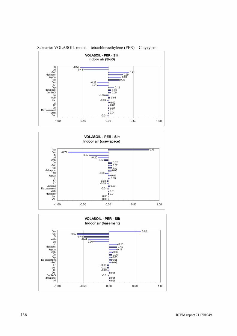
136 RIVM report 711701049
Scenario: VOLASOIL model – tetrachloroethylene (PER) – Clayey soil
VOLASOIL - PER - SiltIndoor air (SloG)
-0.010.010.010.020.020.02
-0.030.04
-0.050.050.06
0.12-0.21-0.22
0.220.26
0.290.41
-0.48-0.56
-1.00 -0.50 0.00 0.50 1.00
Dwvri b
Da basementDaKfz
Lwvrcb
dgDa SloG
delta pcsVpLf
VsVa
kappadelta pic
AofvriS
VOLASOIL - PER - SiltIndoor air (crawlspace)
0.000.00
0.010.01
-0.010.03
-0.03-0.03
0.030.04
-0.060.060.070.070.07
-0.07-0.20
-0.37-0.79
0.79
-1.00 -0.50 0.00 0.50 1.00
DwLw
delta picvri b
Da basementDa SloG
LfKfz
kappadg
delta pcsVp
AofDa
vrcbvriS
VsVa
VOLASOIL - PER - SiltIndoor air (basement)
0.010.01
-0.010.01
-0.02-0.03-0.03
0.050.050.050.060.07
0.140.150.16
-0.30-0.41
-0.49-0.62
0.62
-1.00 -0.50 0.00 0.50 1.00
vridelta pcsDa SloG
DwKf
LwLf
AofDa basement
VpDa
vrcbkappa
delta picz
dgvri b
SVsVa
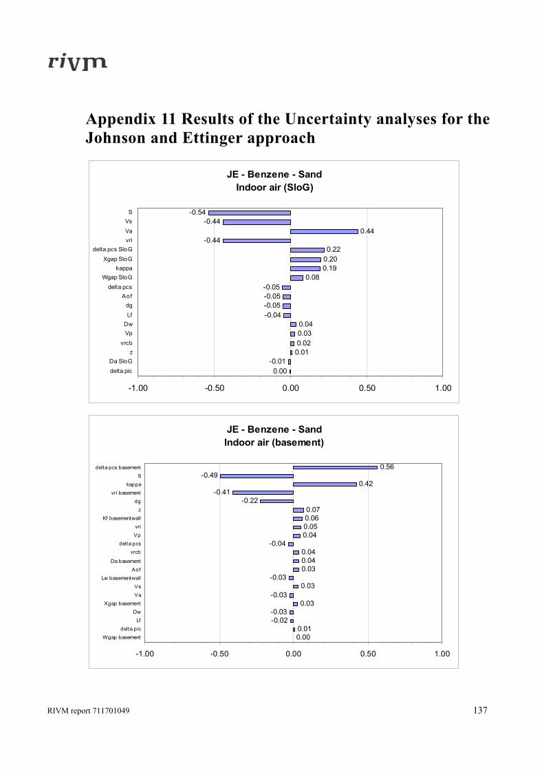
RIVM report 711701049 137
Appendix 11 Results of the Uncertainty analyses for the Johnson and Ettinger approach
JE - Benzene - SandIndoor air (SloG)
0.00-0.01
0.010.020.030.04
-0.04-0.05-0.05-0.05
0.080.190.200.22
-0.440.44
-0.44-0.54
-1.00 -0.50 0.00 0.50 1.00
delta picDa SloG
zvrcb
VpDwLfdg
Aofdelta pcs
Wgap SloGkappa
Xgap SloGdelta pcs SloG
vriVa
VsS
JE - Benzene - SandIndoor air (basement)
0.000.01
-0.02-0.03
0.03-0.03
0.03-0.03
0.030.040.04
-0.040.040.050.060.07
-0.22-0.41
0.42-0.49
0.56
-1.00 -0.50 0.00 0.50 1.00
Wgap basementdelta pic
LfDw
Xgap basementVaVs
Lw basementwallAof
Da basement
vrcbdelta pcs
Vpvri
Kf basementwallz
dgvri basement
kappaS
delta pcs basement
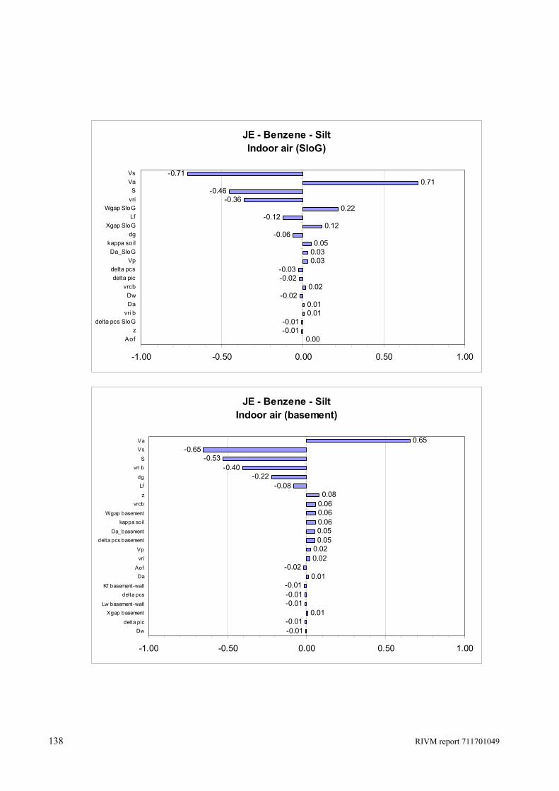
138 RIVM report 711701049
JE - Benzene - SiltIndoor air (SloG)
0.00-0.01-0.01
0.010.01
-0.020.02
-0.02-0.03
0.030.030.05
-0.060.12
-0.120.22
-0.36-0.46
0.71-0.71
-1.00 -0.50 0.00 0.50 1.00
Aofz
delta pcs SloGvri b
DaDw
vrcbdelta pic
delta pcsVp
Da_SloGkappa so il
dgXgap SloG
LfWgap SloG
vriS
VaVs
JE - Benzene - SiltIndoor air (basement)
-0.01-0.01
0.01-0.01-0.01-0.01
0.01-0.02
0.020.020.050.050.060.060.060.08
-0.08-0.22
-0.40-0.53
-0.650.65
-1.00 -0.50 0.00 0.50 1.00
Dwdelta pic
Xgap basementLw basement-wall
delta pcsKf basement-wall
DaAof
vriVp
delta pcs basementDa_basement
kappa soilWgap basement
vrcbz
Lfdg
vri bS
VsVa
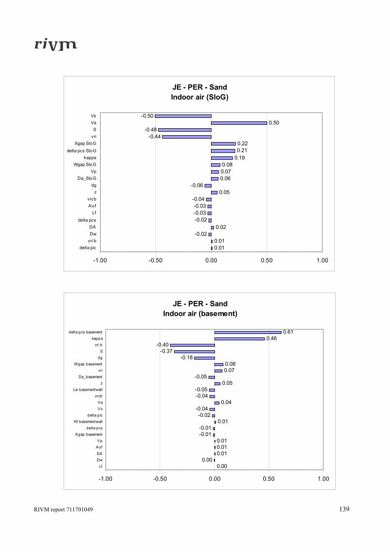
RIVM report 711701049 139
JE - PER - SandIndoor air (SloG)
0.010.01
-0.020.02
-0.02-0.03-0.03-0.04
0.05-0.06
0.060.070.08
0.190.210.22
-0.44-0.48
0.50-0.50
-1.00 -0.50 0.00 0.50 1.00
delta picvri bDwDA
delta pcs
LfAofvrcb
zdg
Da_SloGVp
Wgap SloGkappa
delta pcs SloGXgap SloG
vriS
VaVs
JE - PER - SandIndoor air (basement)
0.000.00
0.010.010.01
-0.01-0.01
0.01-0.02
-0.040.04
-0.04-0.05
0.05-0.05
0.070.08
-0.18-0.37
-0.400.46
0.61
-1.00 -0.50 0.00 0.50 1.00
LfDwDAAofVp
Xgap basementdelta pcs
Kf basementwalldelta pic
VsVa
vrcbLw basementwall
zDa_basement
vriWgap basement
dgS
vri bkappa
delta pcs basement
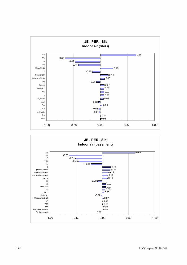
140 RIVM report 711701049
JE - PER - SiltIndoor air (SloG)
0.000.01
-0.03-0.03
0.03-0.03
0.060.060.070.070.07
-0.080.08
0.14-0.15
0.23-0.41
-0.47-0.66
0.66
-1.00 -0.50 0.00 0.50 1.00
vrcb
Da
delta pic
vri b
DwAof
Da_SloG
z
Vp
delta pcs
kappa
dgdelta pcs SloG
Xgap SloG
Lf
Wgap SloG
vri
S
Vs
Va
JE - PER - SiltIndoor air (basement)
0.000.000.000.010.010.02
-0.020.030.050.070.07
-0.090.100.110.12
0.150.16
-0.21-0.45
-0.51-0.63
0.63
-1.00 -0.50 0.00 0.50 1.00
Da_basementLw basementwall
DwAof
vriKf basementwall
delta picvrcb
Dadelta pcs
VpLf
kappadelta pcs basement
Wgap basementXgap basement
zdg
vri bS
VsVa

RIVM
National Institute
for Public Health
and the Environment
P.O. Box 1
3720 BA Bilthoven
The Netherlands
www.rivm.com