Risk Modeling

Defining Risk as Standard Deviation• That’s what Harry Markowitz used.• It has several important and useful properties:

– Symmetric

– Well-understood statistical properties.

– Machinery exists for aggregation from asset to portfolio.

– Predictable

2 TP P P h V h

IssuesMagellan Fund

J anuary 1973 - September 1994

0.00%

5.00%

10.00%

15.00%

20.00%

25.00%

30.00%

35.00%

40.00%

-25% -20% -15% -10% -5% 0% 5% 10% 15% 20%

Return

• Non-normal distributions– Fat tails

(kurtosis)

– Skewness

• Other choices:– Semivariance

– Shortfall probability

– Value at Risk

Why Risk Models?

• Let’s look at how we aggregate portfolio risk:

• For N assets, we require N(N+1)/2 parameters. If N=1,000, we need to estimate 500,500 parameters.

• That is the challenge.

2

2 2 2 2 2 21 1 2 2

1 2 12 1 3 13 1 1,2 2 2

TP P

N N

N N N N

h h h

h h h h h h

h V h

Historical Risk

• This is the most straight forward approach. Why doesn’t it work?

• Observe N asset returns over T periods. We estimate:

• What are the problems with doing this?

1

1ˆ

1

T

ij i i j jt

r t r r t rT

Problems with historical risk• Let’s think about the number of parameters.• We need to estimate N(N+1)/2 parameters, and we have

NT observations. We require at a minimum, 2 observations per parameter estimate. (How can we estimate a variance from 1 number?)

• Hence, NTN(N+1), or T>N. This causes problems when we are looking at monthly returns for 1,000 assets.– Technical version: unless T>N, we will estimate a singular

covariance matrix. What does that mean, mathematically? Intuitively?

• And even if we had 1,000 months of data (or more), we know that assets and markets change over time. We also regularly observe new assets. We don’t have 1,000 months of data on Google.

Single Factor Model

• Simplified version of Sharpe’s Market Model

• Decompose returns into market and active components.

• Postulate that active components are uncorrelated.

2

21

22

2

0 0

0

0

mkt

Tmkt

N

r

r e δ

V e e Δ

Δ

Single Factor Model

• Solves the number of parameters problem:– For N assets, it requires N+1 parameters.– N active risks, 1 market volatility.

• Problem with this model: it doesn’t capture observed correlation structure in the market. Are Exxon and Chevron correlated only through their market exposure?

• Advantage: simplicity makes this useful for back-of-the-envelope calculations.

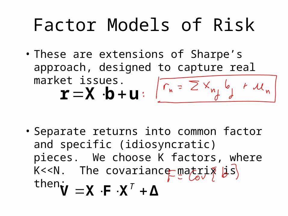
Factor Models of Risk

• These are extensions of Sharpe’s approach, designed to capture real market issues.

• Separate returns into common factor and specific (idiosyncratic) pieces. We choose K factors, where K<<N. The covariance matrix is then:

r X b u

T V X F X Δ

Choosing the Factors

• Art not science.• Three general approaches:

– Fundamental factors (BARRA, Northfield)• Industries and investment themes.

– Macroeconomic factors (Salomon RAM, BIRR model)• Industrial productivity, inflation, interest rates, oil prices…

– Statistical factors (Quantal, Northfield)• Use statistical factor modeling, principal components

analysis…

• These three approaches involve different estimation issues, and exhibit different levels of effectiveness.

Fundamental Models

• Typically about 60 factors for a major equity market.

• Calculate factor exposures, X, from fundamental data.– Industry membership.

– Risk index exposures (e.g. value based on B/P)

• Run monthly cross-sectional GLS regressions to estimate factor returns.

• Use N observations to estimate K factor returns.

11 1 T Tb X Δ X X Δ r

Aside: Factor Portfolios

• Our extensive use of fundamental models makes it worth understanding factor portfolios in more detail.

• We estimate factor returns as:

• This equation has the form:

• Each estimated factor return, bj, is a weighted sum of asset returns. We can interpret those weights as the asset weights in a factor portfolio, or factor-mimicking portfolio.

11 1 T Tb X Δ X X Δ r

T b H r

Factor Portfolios• The columns of H contain the portfolio weights, with one

column for each factor.• The GLS estimation approach guarantees that factor

portfolio-j has:– Unit exposure to factor-j– Zero exposure to all other factors.– Minimum risk.

• Industry factor portfolios are typically fully invested, with long and short positions.

• Risk index factor portfolios are typically net zero investments, with positions in every stock.

• We will find factor portfolios quite useful later in this course.

Macroeconomic Models

• Typically about 9 factors for a major equity market.

• Calculate the change (or shock) in each macrovariable each month.

• Estimate exposure to such shocks, stock by stock, using time-series data.

• This approach requires NK parameter estimates.

1

K

n k nk nk

r t b t X t

Statistical Models

• Start with only returns data.• Use statistical analysis to determine number and

identity of most important factors.– While this approach sounds completely objective, it

involves many subjective decisions, e.g. choosing portfolios to build an initial historical covariance matrix.

• This approach implicitly assumes that factor exposures are constant over estimation period.

• Factors change from month to month.

Performance and Uses*• Fundamental models

– In general, best risk forecasting out-of-sample, but dependent on choosing the right factors.

– Intuitive factors also useful for performance attribution and alpha forecasting.

• Macroeconomic models:– Poor at risk forecasting.– Direct macroeconomic connections can be useful for alpha forecasting.

• Statistical models:– Best in-sample forecasts. Will outperform fundamental models with

poorly chosen factors.– Misses factors whose exposures change over time (especially

momentum).– Not useful for performance attribution. Difficult to use for alpha

forecasting.

*See Gregory Connor, “The Three Types of Factor Models: A Comparison of their Explanatory Power.” Financial Analysts Journal, May-June 1995, pp. 42-46.

Covariance Matrix Estimation

• For fundamental and macroeconomic models (and even to some extent for statistical models), we still need to estimate the covariance matrix, given the factor return history.

• We also need to estimate the specific (idiosyncratic) risk matrix.

An Example

• Want best forecast of portfolio risk over the next several months. (Horizon will depend on use.)

• Given that risk varies over time, we would like to overweight more recent observations.

• At the same time, we have the parameter estimation challenge: we want T>>K. Lowering the weight on historical observations effectively lowers T.

• Here is one approach.

US Equity Covariance Matrix

• Historical monthly data back to 1973. Between 65 and 70 factors.

• Step 1: Use exponential smoothing to estimate factor covariance matrix:

1

1

1ˆ 1

1

T

i i j jt

ij T

t

r t r r t r Exp T tT

T Exp T t

Step 2: Specific Risk Model

• Our monthly factor return estimations also estimate specific returns:

• We could calculate historical specific risk. Instead we estimate the following model:

• We build models for S and v.– What are the estimation issues around this?

r X b u

2

2

1

1

1

n n

N

nn

u t S t v t

S t u tN

A Very Useful Property

• We have occasion to invert the covariance matrix, i.e.

• This is typically an operation of order N3.

• If the covariance matrix has the factor form, then:

• Why is this useful?

1 1, V α V e

11 1 1 1 1 1T T V Δ Δ X X Δ X F X Δ

Testing Risk Forecasts

• Given r(t) and (t), how can we test whether (t) is a good risk forecast?

• Bias test:– Convert returns to standardized outcomes:

– The bias statistic is the sample standard deviation of these outcomes:

– If the bias>1, we have under-predicted risk, and vice versa.

r tx t

t

| 1,bias StDev x t t T

Testing Risk Forecasts

• Statistical significance: Remember that for normally distributed random numbers:

• The bias test estimates whether we are accurate on average. We can apply it to total, residual, common factor, and specific risk.

• We can use further tests to see if our forecasts are above average when realized risk is above average, etc.

2

SET

Total and Active Risk

• Given the covariance matrix, we can estimate total and active risk:

• We can also estimate the correlation of returns from two portfolios:

2

2

T T TP P P P P P P

T T TP PA PA PA PA PA PA

h V h x F x h Δ h

h V h x F x h Δ h

,TA B

A BA B

Corr r r

h V h

Beta

• The CAPM has given beta an exalted role, and implied that beta is uniquely defined:

– I will assume you know the CAPM already.

• As active managers, we will view the CAPM as a source of consensus expected returns:

– This is what investors on average are expecting, not what we expect.

P P B Pr r

consP P Bf f

Beta

• We often think of estimating betas using time-series regressions.

,

P B

P B

B

r t r t t

Cov r r

Var r

Beta

• In that regression view, we estimate the covariance and variance using the observed time-series.

• But given our covariance matrix, which is a forward-looking forecast, we can (hopefully) develop a better beta forecast:

• These were Barr’s better betas.

2 2,

TTP B BP

B B

h V h V h

h β β

Barr Rosenberg

Marginal Contributions

• It is often useful to know at the margin the significant contributors to risk:

• Why is this useful? Remember first order portfolio construction conditions:

P PTP P

P PATPA P

V hMCTR

h

V hMCAR

h

2 PA α V h

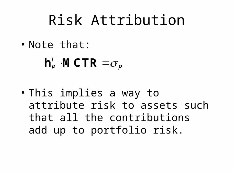
Risk Attribution

• Note that:

• This implies a way to attribute risk to assets such that all the contributions add up to portfolio risk.

TP P h MCTR