Risk Management for Catastrophe Loss

Jin-Ping Lee and Min-Teh Yu∗

October 30, 2007

Abstract

This study investigates the valuation models for three types of catastrophe-linkedinstruments: catastrophe bonds, catastrophe equity puts, and catastrophe futures andoptions. First, it looks into the pricing of catastrophe bonds under stochastic interestrates and examines how reinsurers can apply catastrophe bonds to reduce the defaultrisk. Second, it models and values the catastrophe equity puts that give the (re)insurerthe right to sell its stocks at a predetermined price if catastrophe losses surpass atrigger level. Third, this study models and prices catastrophe futures and catastropheoptions contracts that are based on a catastrophe index.

KeyWords: Catastrophe Risk, Catastrophe Bond, Catastrophe Equity Put, Catastro-phe Futures Options, Contingent Claim Analysis.

JEL classification: G20, G28, G21

∗Lee: Associate Professor, Department of Finance, Feng Chia University, Taichung, Taiwan. Fax: 886-4-24513796, Email: jplee@fcu.edu.tw. Yu: Professor, Department of Finance, Providence University, Taichung43301, Taiwan. Tel.: 886-4-26310631, Fax: 886-4-26311170, Email: mtyu@pu.edu.tw.

1

1 Introduction

Catastrophic events having low frequency of occurrence but generally high loss severity

can easily erode the underwriting capacity of property and casualty insurance and reinsur-

ance companies (P&Cs, hereafter). P&Cs traditionally hedge catastrophe risks by buying

catastrophe reinsurance contracts. Because of capacity shortage and constraints in the rein-

surance markets, the capital markets develop alternative risk transfer instruments to provide

(re)insurance companies with vehicles for hedging their catastrophe risk. These instruments

can be broadly classified into three categories: insurance-linked debt contracts (e.g. catastro-

phe bonds), contingent capital financing instruments (e.g. catastrophe equity puts), and

catastrophe derivatives (e.g. catastrophe futures and catastrophe options).

The Chicago Board of Trade (CBOT) launched catastrophe (CAT) futures in 1992 and

CAT futures call spreads in 1993 with contract values linked to the loss index compiled by

the Insurance Services Office. The CBOT switched to CAT options in 1995 to try to spur

growth in the CAT derivatives market, but was unable to generate meaningful activity and

ultimately abandoned it in 2000. The CAT bonds, however, have been quite successful

with 89 transactions completed, representing $15.53 billion in issuance since the first issue

in 1997.1 Since 1996, several CAT equity put deals were negotiated usually with obligations

to purchase stock of $100 million each.

This study looks into the valuation models for these CAT-linked instruments and exam-

ines how their values are related to catastrophe risk, terms of the contract, and other key

elements of these instruments. The rest of this study is organized into four sections. Sec-

tion II provides a model to value catastrophe bonds under stochastic interest rates. Section

III models and values the catastrophe equity puts with credit risk, and section IV models

and prices catastrophe futures and catastrophe options contracts that are based on specified

1See MMC Security (2007).

2

catastrophe indices. Section V investigates how reinsurers can apply catastrophe bonds to

reduce their default risk. This study’s valuation approach employs the contingent claim

analysis, and when a closed-form solution cannot be derived numerical estimates will be

computed using the Monte Carlo simulation method.

2 Catastrophe bonds

The CAT bond, which is also named as an ”Act of God bond”, is a liability-hedging instru-

ment for insurance companies. There are debt-forgiveness triggers in CAT bond provisions,

whereby the generic design allows for the payment of interest and/or the return of principal

forgiveness, and the extent of forgiveness can be total, partial, or scaled to the size of the

loss. Moreover, the debt forgiveness can be triggered by the (re)insurer’s actual losses or on

a composite index of insurers’ losses during a specific period. The advantage of a CAT bond

hedge for (re)insurers is that the issuer can avoid the credit risk. The CAT bondholders

provide the hedge to the (re)insurer by forgiving existing debt. Thus, the value of this hedge

is independent of the bondholders’ assets and the issuer has no risk of non-delivery on the

hedge. However, from the bondholder’s perspective, the default risk, the potential moral

hazard behavior, and the basis risk of the issuing firm are critical in determining the value

of CAT bonds.

2.1 CAT bond valuation models

Litzenberger et al. (1996) considered a one-year bond with an embedded binary CAT option.

The repayment of principal is indexed to the (re)insurer’s catastrophe loss (denoted as CT ).

This security may be decomposed into two components: (1) long a bond with a face value

of F and (2) short a binary call on the catastrophe loss and with a strike price K. Under

the assumption that the natural logarithm of the catastrophe loss is normally distributed,

the one-year CAT bond can be priced as follows:

3

PCAT = e−rT × (F − Φ [−zK ]× POT ) , (1)

zK =log(K)− u

σ.

Here, r is the risk free interest rate; µ and σ are respectively the mean and standard deviation

of ln(CT ); Φ(·) denotes the cumulative distribution function for a standard normal random

variable; POT refers to the option’s payout at maturity date, T . For a CAT call option

spread, when the (re)insurer’s catastrophe loss (CT ) is less than K1, the bondholder receives

a repayment of the entire principal; when the loss is between K1 and K2 (where K2 > K1),

the fraction of principal lost is (C−K1)(K2−K1)

; and for the loss greater than K2, the entire principal

payment is lost.

This security may be divided into two components: (1) long a bond with an above-market

coupon (c) and (2) a CAT call option spread consisting of a short position on the CAT call

with a strike price of K1 and a long position on the CAT call with a strike price of K2. Under

the assumption that the (re)insurer’s catastrophe loss is lognormally distributed with mean

µ and standard deviation σ, the CAT bond can be priced as follows:

PCAT = e−rT × F ×

⎛⎜⎜⎝ 1− Φ [−zK1]×∙eµ+

12σ2 × Φ[−zK1

+σ]Φ[−zK1]

−K1

¸+Φ [−zK2 ]×

∙eµ+

12σ2 × Φ[−zK2

+σ]Φ[−zK2 ]

−K2

¸⎞⎟⎟⎠ (2)

zKi =log(Ki)− u

σ. i = 1, 2.

Litzenberger et al.(1996) provided a bootstrap approach to price these hypothetical CAT

bonds and compared them with the prices calculated under the assumption of the lognormal-

ity of catastrophe loss distribution. Zajdenweber (1998) followed Litzenberger et al. (1996),

but changed the CAT loss distribution to the stable-Levy distribution. Contrary to Litzen-

berger et al. (1996) and Zajdenweber (1998), there were a series of attempts to relax the

interest rate assumption to be stochastic. For instance, Loubergé et al. (1999) numerically

4

estimated the CAT bond price by assuming the interest rate follows a binomial random

process and the catastrophe loss a compound Poisson process.

Lee and Yu (2002) extended the literature and priced CAT bonds with a formal term

structure model of Cox et al. (1985). Under the setting that the aggregate loss is a compound

Poisson process, a sum of jumps, the aggregate catastrophe loss facing the (re)insurer i can

be described as follows:

Ci,t =

N(t)Xj=1

Xi,j, (3)

where the process {N(t)}t≥0 is the loss number process, which is assumed to be driven

by a Poisson process with intensity λ. Terms Xi,j denote the amount of losses caused

by the jth catastrophe during the specific period for the issuing (re)insurance company.

Here, Xi,j , for j = 1, 2, ..., N(T ), are assumed to be mutually independent, identical, and

lognormally-distributed variables, which are also independent of the loss number process,

and their logarithmic means and variances are µi and σ2i , respectively.

A discount bond whose payoffs (POT ) at maturity (i.e. time T) can be specified as

follows:

POT =

½F if CT ≤ Krp× F if CT > K,

(4)

where K is the trigger level set in the CAT bond provisions, Ci,T is the aggregate loss at

maturity, rp is the portion of principal needed to be paid to bondholders when the forgiveness

trigger has been pulled, and F is the face value of the CAT bond. Under the assumption

that the term structure of interest rates is independent of the catastrophe risk, the CAT

bond can be priced as follows:

PCAT = PCIR(0, T )× [∞Xj=0

e−λT(λT )j

j!F j(K) + rp(1−

∞Xj=0

e−λT(λT )j

j!F j(K)], (5)

where

F j(K) = Pr(Xi,1 +Xi,2 + ...+Xi,j ≤ K)

5

denotes the jth convolution of F , and

PCIR(0, T ) = A(0, T )e−B(0,T )r(0),

where

ACIR(0, T ) = [2γe(κ+γ)

T2

(κ+ γ)(eγT − 1) + 2γ ]2κmv2

B(0, T )CIR =2(eγT − 1)

(γ + κ)(eγT − 1) + 2γ

γ =√κ2 + 2v2.

Here, κ is the mean-reverting force measurement, and v is the volatility parameter for the

interest rate.

2.1.1 Approximating An Analytical Solution

Under the assumption that the catastrophe loss amount is independent and identically

lognormally-distributed, the exact distribution of the aggregate loss at maturity, denoted

as f(Ci,T ), cannot be known. Lee and Yu (2002) approximated the exact distribution by

a lognormal distribution, denoted as g(Ci,T ), with specified moments.2 Following the ap-

proach, the first two moments of g(Ci,T ) are set to be equal to those of f(Ci,T ), which can

be written as:

µg = E[Ci,T ] = λTeµX+12σ2X (6)

σ2g = V ar[Ci,T ] = λTe2µX+2σ2X , (7)

where µg and σ2g denote the mean and variance of the approximating distribution g(Ci,T ),

respectively. The price of the approximating analytical CAT bond can be shown to be the

following:

PCIR(0, T )

∙Z K

0

1√2πσgCi,T

e−12(lnCi,T−µg)

2

dCi,T + rp

Z ∞

K

1√2πσgCi,T

e−12(lnCi,T−µg)

2

dCi,T

¸.

(8)

2Jarrow and Rudd (1982), Turnbull and Wakeman (1991), and Nielson and Sandmann (1996) used thesame assumption in approximating the values of Asian options and basket options.

6

We report the results of Lee and Yu (2002) in Table 1 to illustrate the difference between

the analytical estimates and numerical estimates. Table 1 shows that the values of the

approximating solution and the values from the numerical method are very close and within

the range of 10 basis points for most cases. In addition, the approximate CAT bond prices

are higher than those estimated by the Monte Carlo simulations for a high value of σi. This is

because the approximate lognormal distribution underestimates the tail probability of losses

and this underestimation is more significant when σi is high. We also note that the CAT

bond price increases with trigger levels and this increment rises with occurrence intensity

and loss variance.

2.1.2 Default-Risky CAT Bonds

In order to look into the practical considerations of default risk, basis risk, and moral hazard

relating to CAT bonds, Lee and Yu (2002) developed a structural model in which the insurer’s

total asset value consists of two risk components - interest rate and credit risk. The term

credit risk refers to all risks that are orthogonal to the interest rate risk. Specifically, the

value of an insurer’s assets is governed by the following process:

dVtVt= µV dt+ φdrt + σV dWV,t, (9)

where Vt is the value of the insurer’s total assets at time t; rt is the instantaneous interest

rate at time t;WV,t is the Wiener process that denotes the credit risk; µA is the instantaneous

drift due to the credit risk; σV is the volatility of the credit risk; and φ is the instantaneous

interest rate elasticity of the insurer’s assets.

In the case where the CAT bondholders have priority for salvage over the other debthold-

ers, the default-risky payoffs of CAT bonds can be written as follows:

POi,T =

⎧⎨⎩ a ∗ L if Ci,T ≤ K and Ci,T ≤ Vi,T − a ∗ Lrp ∗ a ∗ L if K < Ci,T ≤ Vi,T − rp ∗ a ∗ LMax {Vi,T − Ci,T , 0} otherwise,

(10)

7

where POi,T are the payoffs at maturity for the CAT bond forgiven on the issuing firm’s

own actual losses; Vi,T is the issuing firm’s asset value at maturity; Ci,T is the issuing firm’s

aggregate loss at maturity; a is the ratio of the CAT bond’s face amount to total outstanding

debts (L). According to the payoff structures in POi,T and the specified asset and interest

rate dynamics, the CAT bonds can be valued as follows:

Pi =1

a ∗ LE∗0 [e

−r̄TPOi,T ], (11)

where Pi is the default-risky CAT bond price with no basis risk. Term E∗0 denotes expecta-

tions taken on the issuing date under risk-neutral pricing measure; r̄ is the average risk-free

interest rate between issuing date and maturity date; and 1a∗L is used to normalize the CAT

bond prices for a $1 face amount.

2.1.3 Moral hazard and basis risk

Moral hazard results from less loss-control efforts by the insurer issuing CAT bonds, since

these efforts may increase the amount of debt that must be repaid at the expense of the

bondholders’ coupon (or principal) reduction. Bantwal and Kunreuther (2000) noted the

tendency for insurers to write additional policies in the catastrophe-prone area, spending

less time and money in their auditing of losses after a disaster.

Another important element that needs to be considered in pricing a CAT bond is the

basis risk. The CAT bond’s basis risk refers to the gap between the insurer’s actual loss and

the composite index of losses that makes the insurer not receive complete risk hedging. The

basis risk may cause insurers to default on their debt in the case of high individual loss, but

a low index of loss. There is a trade-off between basis risk and moral hazard. If one uses an

insurer’s actual loss to define the CAT bond payments, then the insurer’s moral hazard is

reduced or eliminated, but basis risk is created.

In order to incorporate the basis risk into the CAT bond valuation, aggregate catastrophe

losses for a composite index of catastrophe losses (denoted as Cindex,t) can be specified as

8

follows:

Cindex,t =

N(t)Xj=1

Xindex,j, (12)

where the process {N(t)}t≥0 is the loss number process, which is assumed to be driven by

a Poisson process with intensity λ. Terms Xindex,j denote the amount of losses caused by

the jth catastrophe during the specific period for the issuing insurance company and the

composite index of losses, respectively. Terms Xindex,j, for j = 1, 2, ..., N(T ), are assumed

to be mutually independent, identical, and lognormally-distributed variables, which are also

independent of the loss number process, and their logarithmic means and variances are µindex

and σ2index, respectively. In addition, the correlation coefficients of the logarithms of Xi,j and

Xindex,j, for j = 1, 2, ..., N(T ) are equal to ρX .

In the case of the CAT bond being forgiven on the composite index of losses, the default-

risky payoffs can be written as:

POindex,T =

⎧⎨⎩ a ∗ L if Cindex,T ≤ K and Ci,T ≤ Vi,T − a ∗ Lrp ∗ a ∗ L if Cindex,T > K and Ci,T ≤ Vi,T − rp ∗ a ∗ LMax {Vi,T − Ci,T , 0} otherwise,

(13)

where Cindex,T is the value of the composite index at maturity, and a, L, rp, Vi,T , Ci,T , and

K are the same as defined in equation (10). In the case where the basis risk is taken into

account the CAT bonds can be valued as follows:

Pindex =1

a ∗ LE∗0 [e

−r̄TPOindex,T ], (14)

where Pindex is the default-risky CAT bond price with basis risk at issuing time. Terms E∗0 ,

r̄ , and 1a∗L are the same as defined in equation (11).

The issuing firm might relax its settlement policy once the accumulated losses fall into

the range close to the trigger. This would then cause an increase in expected losses for the

next catastrophe. This change in the loss process can be described as follows:

µ0i =

½(1 + α)µi if (1− β)K ≤ Ci,j ≤ K,µi otherwise,

(15)

9

where µ0i is the logarithmic mean of the losses incurred by the (j+1)th catastrophe when the

accumulated loss Ci,j falls in the specified range, (1− β)K ≤ Ci,j ≤ K. Term α is a positive

constant, reflecting the percentage increase in the mean, and β is a positive constant, which

specifies the range of moral hazard behavior.

We expect that both moral hazard and basis risk will drive down the prices of CAT

bonds. The results of the effects of moral hazard and basis risk on CAT bonds can be found

in Lee and Yu (2002). The significant price differences indicate that the moral hazard is an

important factor and should be taken into account when pricing the CAT bonds.3 A low

loss correlation between the firm’s loss and the industry loss index subjects the firm to a

substantial discount in its CAT bond prices.

3 Catastrophe equity puts

If a insurer suffers a loss of capital due to a catastrophe, then its stock price is likely to

fall, lowering the amount it would receive for newly issued stock. Catastrophe equity puts

(CatEPut) give insurers the right to sell a certain amount of its stock to investors at a

predetermined price if catastrophe losses surpass a specified trigger.4 Thus, catastrophe

equity puts can provide insurers with additional equity capital when they need funds to

cover catastrophe losses. A major advantage of catastrophe equity puts is that they make

equity funds available at a predetermined price when the insurer needs them the most.

However, the insurer that uses catastrophe equity puts faces a credit risk - the risk that the

seller of the catastrophe equity puts will not have enough cash available to purchase the

insurer’s stock at the predetermined price. For the investors of catastrophe equity puts they

also face the risk of owning shares of a insurer that is no longer viable.

3Bantwal and Kunreuther (2000) also pointed out that moral hazard may explain the CAT bond premiumpuzzle .

4Catastrophe equity puts, or CatEPuts, are underwritten by Centre Re and developed by Aon with CentreRe.

10

3.1 Catastrophe equity put valuation models

The CatEPut gives the owner the right to issue shares at a fixed price, but that right

is only exercisable if the accumulated catastrophe losses exceed a trigger level during the

lifetime of the option. Such a contract is a special "double trigger" put option. Cox et al.

(2004) valued a CatEPut by assuming that the price of the insurer’s equity is driven by a

geometric Brownian motion with additional downward jumps of a specified size in the event

of a catastrophe.

The price of the insurer’s equity can be described as:

St = S0 exp

µ−ANt + σWt +

∙µS −

1

2σ2S

¸t

¶, (16)

where St denotes the equity price at time t; {W}t≥0 is a standard Brownianmotion; {N(t)}t≥0

is the loss number process, which is assumed to be driven by a Poisson process with intensity

λS; A ≥ 0 is the factor to measure the impact of catastrophe on the market price of the

insurer’s equity; and µS and σS are respectively the mean and standard deviation of return

on the insurer’s equity given that no catastrophe occurs during an interval. The option is

exercisable only if the number of catastrophes occurring during the lifetime of the contract

is larger than a specified number (denoted as n). The payoffs of the CatEPut at maturity

can be written as:

POCFP =

½K − ST if ST < K and NT ≥ n0 otherwise

, (17)

where K is the exercise price. This CAT put option can be priced as follows:

PCFP =∞Xj=n

e−λST(λST )

j

j!

³Ke−rTΦ (dj)− S0e

−Aj+kTΦ³dj − σS

√T´´

, (18)

where

k = λS¡1− e−A

¢dj =

log³KS0

´− rT +Aj − kT +

σ2ST

2

σS√T

.

11

Improving upon the assumption of Cox et al. (2004) that the size of the catastrophe is

irrelevant, Jaimungal and Wang (2006) assumed that the drop in the insurer’s share price

depends on the level of the catastrophe losses and valued the CatEPut under a stochastic

interest rate. Jaimungal and Wang (2006) modeled the process of the insurer’s share price

as follows:

St = S0 exp (−α (L (t)− ϕt) +X (t)) , (19)

whereby

L (t) =

N(t)Xj=1

lj,

dX(t) =

µµS −

1

2σ2S

¶dt+ σSdW

S (t) ,

dr(t) = κ (θ − r (t)) + σrdWr (t) ,

d£WS,W r

¤(t) = ρS,rdt,

where WS (t) andW r (t) are correlated Wiener processes driving the returns of the insurer’s

equity and the short rate, respectively; L (t) denotes the accumulated catastrophe losses

facing the insurer at time t; lj, for j = 1, 2, ..., are assumed to be mutually independent,

identical, and distributed variables representing the size of the jth loss with p.d.f fL (y) and

mean l; {N(t)}t≥0 is a homogeneous Poisson process with intensity λ. The term ϕt is used

to compensate for the presence of downward jumps in the insurer’s share price and is chosen

as:

ϕ =λ

α

Z ∞

0

¡1− e−αy

¢fL (y) dy.

The parameter α represents the percentage drop in the share price per unit of a catastrophe

loss and is calibrated such that:

αE (lj) = δ =⇒ α =δ

l.

12

Since the right is exercisable only if the accumulated catastrophe losses exceed a critical

coverage limit during the lifetime of the option, the payoffs of the CatEPut at maturity can

be specified as:

POJW =

(K − ST if ST < K and L(T ) >

ˆ

L0 otherwise

, (20)

where the parameterˆ

L represents the trigger level of catastrophe losses above which the

issuer is obligated to purchase unit shares. Under these settings, the price of the CatEPut

at the initial date can be described as follows:

P JW = e−λT∞Xj=1

(λT )j

j!

Z ∞

ˆL

f(n)L (y)

©KP (0, T )Φ (−d− (y))− S0e

−α(y−ϕT )Φ (−d+ (y))ªdy,

(21)

where f (n)L (y) represents the n-fold convolution of the catastrophe loss density function f (L);

d± (y) =ln¡StKPV asicek (0, T )

¢− α (y − ϕT )± 1

2

˜

σ2r˜σr (0, T )

,

˜

σ2r (0, T ) = σ2ST +2κρS,rσSσr + σ2r

κ2(T −BV asicek (0, T ))−

σ2r2κ

B2V asicek (0, T ) .

Here, P (0, T ) is a T -maturity zero coupon bond in the Vasicek model:

PV asicek (0, T ) = exp {AV asicek (0, T )−BV asicek (0, T ) r (0)} ,

where

A (0, T )V asicek =

µθ − σ2r

2κ2

¶(BV asicek (0, T )− T )− σ2r

4κB2V asicek (0, T ) ,

BV asicek (0, T ) =1

κ

¡1− e−κT

¢.

3.1.1 Credit risk and CatEPuts

Both Cox et al. (2004) and Jaimungal and Wang (2006) did not consider the effect of credit

risk, the vulnerability of the issuer, on the catastrophe equity puts. Here, we follow Cox et al.

(2004) to assume that the option is exercisable only if the number of catastrophes occurring

13

during the lifetime of the contract is larger than a specified number, and we develop a model

to incorporate the effects of credit risk on the valuation of CatEPuts. Consider an insurer

with m1 shares outstanding that wants to be protected in the event of catastrophe losses

by purchasing m2 units of CatEPuts from a reinsurer. Each CAT put option allows the

insurer the right to sell one share of its stock to the reinsurer at a price of K if the insurer’s

accumulated catastrophe losses during the life of the option exceed a trigger level L. The

payoffs while incorporating the effect of the reinsurer’s vulnerability, POLY , can be written

as:⎧⎨⎩K − ST if ST< K and PL,T≥ n and VRe,T−DRe,T> m2(K − ST )

(K − ST )× (K−ST )m2

(K−ST )m2+DRe,Tif ST< K and PL,T≥ n and VRe,T−DRe,T≤ m2(K − ST )

0 otherwise

,

(22)

where PL,t is the loss number process, which is assumed to be driven by a Poisson process

with intensity λP ; St denotes the insurer’s share price and can be shown as:

Si,t =Vi,t − Li,t

m1, (23)

where Vi,t and Li,t represent the values of the insurer’s assets and liabilities at time t, respec-

tively.

The value dynamics for the insurer’s asset and liability are specified as follows:

dVi,t = (r + µVi)Vi,tdt+ σViVi,tdWVi,t, (24)

dLi,t =³r + µLi − λPe

µyi+12σ2yi

´Li,t−dt+ σLiLi,t−dWLi,t + YPLi ,tLi,t−dPL,t, (25)

where r is the risk-free interest rate; µVi is the risk premium associated with the insurer’s asset

risk; µLi denotes the risk premium for small shocks in the insurer’s liabilities;WVi,t is aWeiner

process denoting the asset risk; WLi,t is a Weiner process summarizing all continuous shocks

that are not related to the asset risk of the insurer; and YPLi ,t is a sequence of independent

and identically-distributed positive random variables describing the percentage change in

14

liabilities in the event of a jump. We assume that ln(YPLi ,t) has a normal distribution with

mean µyi and standard deviation σyi. The term λPeµyi+

12σ2yi offsets the drift arising from the

compound Poisson component YPLi ,tLi,t−dPL,t.

The value dynamics for the reinsurer’s assets (VRe,T ) and liabilities (LRe,T ) are specifically

governed by the following processes:

dVRe,t = (r + µVRe)VRe,tdt+ σVRe

VRe,tdWVRe,t, (26)

dLRe,t =³r + µLRe

− λPeµyRe

+ 12σ2yRe

´LRe,t−dt+σLRe

LRe,t−dWLRe,t+YPLRe,t

LRe,t−dPL,t, (27)

where VRe,t and LRe,t represent the values of the reinsurer’s assets and liabilities at time t,

respectively; r is the risk-free interest rate; µVReis the risk premium associated with the

reinsurer’s asset risk; µLRedenotes the risk premium for continuous shocks in the insurer’s

liabilities; WVRe,t is a Weiner process denoting the asset risk; WLRe,t is a Weiner process

summarizing all continuous shocks that are not related to the asset risk of the reinsurer; and

YPLRe,tis a sequence of independent and identically-distributed positive random variables

describing the percentage change in the reinsurer’s liabilities in the event of a jump. We

assume that ln(YPLRe,t) has a normal distribution with mean µyRe

and standard deviation

σyRe. In addition, assume that the correlation coefficient of ln(YPi,t) and ln(YPLRe,t

) is equal to

ρY . The term λPeµy Re+

12σ2yRe offsets the drift arising from the compound Poisson component

YPLRe,tLRe,t−dPL,t.

According to the payoff structures, the catastrophe loss number process, and the dynamics

for the (re)insurer’s assets and liabilities specified above, the CatEPut can be valued as

follows:

PLY = E∗£e−rT × POLY

¤. (28)

Here, E∗ [•] denotes expectations taken on the issuing date under a risk-neutral pricing

measure.

15

The CAT put prices are estimated by the Monte Carlo simulation. Table 2 presents the

numerical results. It shows that the possibility of a reinsurer’s vulnerability (credit risk)

drives the put price down dramatically. We also observe that the higher the correlation

coefficient of ln(YPi,t) and ln(YPLRe,t) (i.e. ρY ) is, the lower the value of the CatEPut will be.

This implies that the reinsurer with efficient diversification in providing reinsurance coverage

can increase the value of the CatEPut.

4 Catastrophe derivatives

Catastrophe risk for (re)insurers can be hedged by buying exchange-traded catastrophe

derivatives such as catastrophe futures, catastrophe futures options, and catastrophe op-

tions. Exchange-traded catastrophe derivatives are standardized contracts based on specified

catastrophe loss indices. The loss indices reflect the entire P&C insurance industry. The

contracts entitle (re)insurers (the buyers of catastrophe derivatives) a cash payment from the

seller if the catastrophes cause the index to rise above the trigger specified in the contract.

4.1 Catastrophe derivatives valuation models

A general formula for the catastrophe futures price can be developed as in Cox and Schwebach

(1992) as follows:

Ft =1

Q(ALt +E [Yt|Jt]) , (29)

where Q is the aggregate premium paid for in the catastrophe insurance portfolio. Here, Yt

denotes the losses of the catastrophe insurance portfolio which are reported after the current

time t, but included in the settlement value, ALt is the current amount of catastrophe losses

announced by the exchange, and Jt denotes the information available at time t. Cox and

Schwebach further derived the catastrophe futures price by assuming Yt follows a compound

Poisson distribution with a intensity parameter λY . The aggregate losses of a catastrophe

insurance portfolio would be the sum of a random variable of individual catastrophe losses

16

which are independent and identically distributed. In other words, Yt = X1+X2+ ...+XN ,

where X1, X2, ..., XN are mutually independent individual catastrophe losses. According to

these assumptions, the futures price can be described as follows:

Ft =1

QALt + (T − t)λY p1, (30)

where p1 represents the first moment of the individual catastrophe loss distribution, i.e.

p1 = E (Xi). Assuming that the loss of a catastrophe insurance portfolio at maturity (i.e.

YT ) is lognormally distributed, that is, the logarithm of ALTALt

is normally distributed with

mean µ (T − t) and variance σ2 (T − t), the futures price can be described as:

Ft =ALt

Qe

µ(T−t)+σ2(T−t)2 . (31)

In the case where ALT is set to be lognormally distributed, Cox and Schwebach (1992)

presented the value of a catastrophe futures call option with exercise price x, denoted as

CCS, as follows:

CCS =e−r(T−t)

Q

µALte

µ+σ2

2(T−t)

Φ (y1)− xQΦ (y2)

¶, (32)

y1 =log³ALtxQ

´+ µ (T − t) + σ2(T−t)

2

σ√T − t

and y2 = y1 − σ√T − t.

Cummins and Geman (1995) used two different processes to describe the instantaneous

claim processes during the event quarter and the run-off quarter. They argued that the

reporting claims by policyholders are continuous and take only a positive value, hence speci-

fying the instantaneous claim to be a geometric Brownian motion during the run-off quarter.

Moreover, they added a jump process to the process during the event quarter. Consequently,

the two instantaneous claim processes during the event quarter¡t ∈

£0, T

2

¤¢and run-off quar-

ter¡t ∈

£T2, T¤¢can be respectively specified as follows:

dct = ct− (µcdt+ σcdWc,t) + JcdNc,t for t ∈∙0,T

2

¸,

dct = ct³µ0cdt+ σ

0cdWc,t

´for t ∈

∙T

2, T

¸,

17

where ct denotes the instantaneous claim which means that the amount of claims reported

during a small length of time dt is equal to ctdt. Terms µc and µ0c represent the mean of the

continuous part of the instantaneous claims during the event quarter and run-off quarter,

respectively, while σc and σ0c represent the standard deviation of the continuous part of the

instantaneous claims during the event quarter and run-off quarter, respectively. Term Jc

is a positive constant representing the severity of loss jump due to a catastrophe, Nc,t is a

Poisson process with intensity λc, and Wc,t is a standard Brownian motion.

Cummins and Geman (1995) derived a formula to value the futures price at time t as

follows:

Ft =

Z t

0

csds+ ct

Ãexpα(

T2−t)−1α

+ k

!+ Jcλc

Ãexpα(

T2−t)−α

¡T2− t¢− 1

α2

!

+c0 expα0(T2 −t)

Ãexpα

0 T2 −1

α0

!+ Jcλc

Ãexpα(

T2−t)−1α

!Ãexpα

0 T2 −1

α0

!, (33)

where α = µc − ρσc and α0= µ

0c − ρσ

0c. Here, ρ represents the equilibrium market price

of claim level risk and is assumed to be constant over period [0, T ]. Cummins and Geman

(1995) also considered catastrophe call spreads written on the catastrophe loss ratio. The

payoffs of European call spreads at maturity T , denoted as Cspread (S, k1, k2), can be written

as follows:

Cspread (c, k1, k2) =Min

(Max

"100

R T0csds

Qc− k1, 0

#, k2 − k1

), (34)

where k1 and k2 are the exercise prices of the catastrophe call spread and k2 > k1, while Qc is

the premiums earned for the event quarter. Since no close-form solution can be obtained, the

catastrophe call spreads under alternative combinations of exercise prices can be estimated by

Monte Carlo simulation. We report the values of 20/40 call spreads estimated by Cummins

and Geman (1995) in Table 3 to present the effects of parameter values on the value of

catastrophe call spreads.

18

Chang, Chang and Yu (1996) used the randomized operational time approach to trans-

fer a compound Poisson process to a more tractable pure diffusion process and led to the

parsimonious pricing formula of catastrophe call options as a risk-neutral Poisson sum of

Black’s call prices in information time. Chang et al. (1996) assumed catastrophe futures

price changes follow jump subordinated processes in calendar-time. The parent process is

assumed to be a lognormal diffusion directed by a homogenous Poisson process as follows:

dXt

Xt= µXt

dt+ σXtdWXt, (35)

where µXtand σXt are the stochastic calendar-time instantaneous mean and variance, re-

spectively, and:

µXtdt = µXdn (t) (36)

σ2Xtdt = σ2Xdn (t) , (37)

where

dn (t) = 1 if the jump occurs once in dt with probability jXdt, otherwisedn (t) = 0 with probability 1− jXdt.

Since the instantaneous mean and variance of calendar-time futures return, µXtdt and

σ2Xtdt, are linear to random information arrival, the information-time proportional factors,

µX and σ2X , are constant. Substituting equations (36) and (37) into equation (35), the parent

process in information time can be transferred into a lognormal diffusion process:

dXn

Xn= µXdt+ σXdWXn . (38)

According to the model, the value of the information-type European catastrophe call

option with strike price k, denoted as c (X,n, k), can be written as follows:

c (X,n, k) =∞X

m=0

Γ (m, jX)B (XΦ (d1)− kΦ (d2)) , (39)

19

d1 =ln¡Xk

¢+ 1

2σ2Xm

σX√m

, d2 = d1 − σX√m,

where Γ (m, j) = e−jX (T−t)[jX(T−t)]mm!

is the Poisson probability mass function with intensity

jx. Moreover, T − t is the option’s calendar-time maturity, r is the riskless interest rate,

B = e−r(T−t) is the price of a riskless matching bond with maturity T − t, and m denotes

the information time maturity index.

Chang et al. (1996) followed Barone-Adsei and Whaley (1987) for an analytical approx-

imation of the American extension of the Black formula to get the value of the information-

time American catastrophe futures call option with strike price k, denoted as C (X,n, k), as

follows:

C (X,n, k) =∞X

m=0

Γ (m, jX)CB (X,n, k) , (40)

where

CB (X,n, k) =

½e−rm [XΦ (d1)− kΦ (d2)] +A

¡XX∗

¢q, where X ≤ X∗

X − k, where X > X∗ , (41)

A =

µX∗

q

¶(1−BΦ (d1 (X

∗))) ,

d1 (X∗) =

ln¡X∗

X

¢+ 1

2σ2Xm

σX√m

,

q =1 +√1 + 4h

2, and h =

2r

σ2X (1−B).

Here, CB (X,n, k) represents the American extension of the Black formula based on MacMil-

lan’s (1986) quadratic approximation of the American stock options. Moreover, X∗ is the

critical futures price above where the American futures option should be exercised immedi-

ately and is determined by solving:

X∗ − k = e−rm [XΦ (d1)− kΦ (d2)] +A

µX

X∗

¶q

+

µX∗

q

¶(1−BΦ (d1 (X

∗))) .

20

Since a diffusion is a limiting case of a jump subordinated process when the jump arrival

intensity approaches infinity and the jump size simultaneously approaches zero, the pricing

model of Black (1976) is a special case of equations (39) and (40).

Table 4 reports the values of information-time American catastrophe call spreads esti-

mated by Chang et al. (1996). It shows that the Black formula underprices the spread

for the 40/60 case. However, for the 20/40 case, the Black formula overprices when the

maturity is short. Chang et al. (1996) noted that the Black formula is a limiting case of

information-time formula, so that the largest mispricing occurs when the jump intensity j is

set at a low value.

5 Reinsurance with CAT-linked securities

P&Cs traditionally diversify and transfer catastrophe risk through reinsurance arrangements.

The objective of catastrophe reinsurance is to provide protection for catastrophe losses that

exceed a specified trigger level. Dassios and Jang (2003) priced stop-loss catastrophe reinsur-

ance contracts while using the Cox process to model the claim arrival process for catastrophes.

However, in the case of catastrophic events, reinsurers might not have sufficient capital to

cover the losses. Recent studies of the catastrophe reinsurance market have found that these

catastrophe events see limited availability of catastrophic reinsurance coverage in the market.

(Froot, 1999 and 2001; Harrington and Niehaus, 2003). P&C reinsurers can strengthen their

ability in providing catastrophe coverages by issuing CAT-linked instruments. For example,

Lee and Yu (2007) developed a model to value the catastrophe reinsurance while considering

the issuance of CAT bonds.

The amount that can be forgiven by CAT bondholders when the trigger level has been

pulled, δ, can be specified as follows:

δ(C∗) = FCAT − PCAT,T , (42)

21

where PCAT,T is the payoffs of the CAT bond at maturity and is specified as follows:

PCAT,T =

½FCAT if C∗ ≤ KCATbond

rp× FCAT if C∗ > KCATbond. (43)

Here, FCAT is the face value of CAT bonds, and C∗ can be the actual catastrophe loss facing

the reinsurer (denoted as Ci,T , specified by equation (3)) or a composite catastrophe index

(denoted as Cindex,T , specified by equation (12)) which depends on the provision set by the

CAT bond. When the contingent debt forgiven by the CAT bond depends on the actual

losses, there is no basis risk. When the basis risk exists, the payoffs of the reinsurance contract

remain the same except that the contingent savings from the CAT bond, δ(C∗), depending

on the catastrophic-loss index, become δ(Cindex,T ). Since the debt forgiven by the CAT bond

does not depend on the actual loss, the realized losses and savings may not match and may

therefore affect the insolvency of the reinsurer and the value of the reinsurance contract in

a way that differs from that without basis risk. Here, KCATbond denotes the trigger level set

in the CAT bond provision.

In the case where the reinsurer i issues a CAT bond to hedge the catastrophe risk, at

maturity the payoffs of the reinsurance contract written by the reinsurer, denoted by Pb,T ,

can be described as follows:

Pb,T =

⎧⎪⎪⎪⎪⎪⎨⎪⎪⎪⎪⎪⎩

M −A if CRe,T ≥M and ARe,T + δ ≥ DRe,T +M −ACRe,T −A if A ≤ CRe,T < M and ARe,T + δ ≥ DRe,T + CRe,T −A(M−A)(ARe,T+δ)

LT+M−A if CRe,T ≥M and ARe,T + δ < DRe,T +M −A(CRe,T−A)(ARe,T+δ)

LT+CReT−A if M > CRe,T ≥ A and ARe,T + δ < DRe,T + CRe,T −A

0 otherwise,(44)

where ARe,T denotes the reinsurer’s asset value at time t, which is assumed to be governed

by the following process:

dARe,tARe,t

= µARedt+ φARe

drt + σARedWVRe,t, (45)

where µAReand σARe

denote respectively the mean and standard deviation of the reinsure’s

asset return; φAReis the instantaneous interest rate elasticity of the reinsurer’s assets; CRe,T

22

is the catastrophe loss covered by the reinsurance contract; andM and A are respectively the

cap and attachment level arranged in the reinsurance contract. In addition to the liability

of providing catastrophe reinsurance coverage, the reinsurer also faces a liability that comes

from providing reinsurance coverages for other lines. Since the liability represents the present

value of future claims related to the non-catastrophic policies, the value of a reinsurer’s

liability, denoted as DRe,t, can be modeled as follows:

dDRe,t = (rt + µDRe)DRe,tdt+ φDRe

DRe,tdrt + σDReDRe,tdWDRe,t, (46)

where φDReis the instantaneous interest rate elasticity of the reinsurer’s liabilities.

The continuous diffusion process reflects the effects of interest rate changes and other

day-to-day small shocks. Term µDRedenotes the risk premium for the small shock, and

WDRe,t denotes the day-to-day small shocks that pertain to idiosyncratic shocks to the capital

market. In order to incorporate the effect of the interest rate risk on the reinsurer’s assets,

the asset value of the reinsurance company is assumed to be governed by the same process

as defined in equation (10).

Under the term structure assumption of Cox et al. (1985) the rate on line (ROL) or the

fairly-priced premium rate can be calculated as follows:

ROL =1

M −A×E∗0

he−

T0 rsds × Pb,T

i, (47)

where ROL is the premium rate per dollar covered by the catastrophe reinsurance; and

E∗0 denotes the expectations taken on the issuing date under risk-neutral pricing measure.

Table 5 reports ROLs with and without basis risk calculated by Lee and Yu (2007). When

the coefficient of correlation between the individual reinsurer’s catastrophe loss and the

composite loss index, ρX , equals 1, no basis risk exists. The lower the ρc is , the higher the

basis risk the reinsurer has. The difference of ROLs for a contract with ρX = 1 and other

alternative values is the basis risk premium. We note that the basis risk drives down the

23

value of the reinsurance contract and the impact magnitude increases with the basis risk,

catastrophe intensity, and loss volatility. We also note that the basis risk premium decreases

with the trigger level and the reinsurer’s capital position, but increases with catastrophe

occurrence intensity and loss volatility.

6 Conclusion

This study investigates the valuation models for three types of CAT-linked securities: CAT

bonds, CAT equity puts, and exchange-traded CAT futures and options. These three new

types of securities are capital market innovations which securitize the reinsurance premiums

into tradable securities and share the (re)insurers’ catastrophe risk with investors.

The study demonstrates how prices of CAT-linked securities can by valued by using a

contingent-claim framework and numerical methods via risk-neutral pricing techniques. It

begins with introducing a structural model of the CAT bond that incorporates stochastic

interest rates and allows for endogenous default risk and shows how its price can be estimated.

The model can also evaluate the effect of moral hazard and basis risk related to the CAT

bonds. This study then extends the literature by setting up a model for valuing CAT

equity puts in which the issuer of the puts is vulnerable. The results show how the values

of CAT equity puts change with the issuer’s vulnerability and the correlation between the

(re)insurer’s individual catastrophe risk and the catastrophe index. Both results indicate

that the credit risk and the basis risk are important factors in determining CAT bonds and

CAT equity puts. This study also compares several models in valuing CAT futures and

options. Though differences exist in alternative models, model prices are within reasonable

ranges and similar patterns are observed on price relations with the underlying elements.

The hedging effect for a reinsurer issuing CAT bonds is also examined.

As long as the threat that natural disasters pose to the financial viability of the P&C

24

industry continues to exist, there is a need for further innovations on better management

of catastrophe risk. The analytical framework in this study in fact provides a platform for

future research on CAT losses with more sophisticated products, contacts, and terms.

References

[1] Bantwal, V. J., and H. C. Kunreuther, 2000, A CAT Bond Premium Puzzle?, Journal

of Psychology and Financial Markets 1(1), 76-91.

[2] Barone-Adesi, G. and R. E. Whaley, 1987, Efficient Analytic Approximation of Ameri-

can Option Values, Journal of Finance 42(2), 301-320.

[3] Black, F., 1976, The Pricing of Commodity Contracts, Journal of Financial Economics

3, 167-179.

[4] Chang, Carolyn., Jack S. Chang and M.-T. Yu, 1996, Pricing Catastrophe Insurance

Futures Call Spreads: A Randomized Operational Time Approach, Journal of Risk and

Insurance 63, 599-617.

[5] Cox, J., J. Ingersoll and S. Ross, 1985, The Term Structure of Interest Rates, Econo-

metrica 53, 385-407.

[6] Cox, S. H., J. R. Fairchild and H. W. Pederson, 2004, Valuation of Structured Risk

Management Products, Insurance: Mathematics and Economics 34, 259-272.

[7] Cox, S. H. and R. G. Schwebach, 1992, Insurance Futures and Hedging Insurance Price

Risk, Journal of Risk and Insurance 59, 628-644.

[8] Cummins, J. D. and H. Geman, 1995, Pricing Catastrophe Futures and Call Spreads:

An Arbitrage Approach, Journal of Fixed Income, March, 46-57.

25

[9] Dassios, Angelos and Ji-Wook Jang, 2003, Pricing of Catastrophe Reinsurance and

Derivatives Using the Cox Process with Shot Noise Intensity, Finance and Stochastics

7(1), 73-95.

[10] Froot, K. A. (Ed.), 1999, The Financing of Catastrophe Risk, University of Chicago

Press, Chicago.

[11] Froot, K. A., 2001, The Market for Catastrophe Risk: A Clinical Examination, Journal

of Financial Economics 60(2) , 529-571.

[12] Harrington, S. E. andG. Niehaus, 2003, Capital, Corporate Income Taxes, and Catastro-

phe Insurance, Journal of Financial Intermediation 12(4), 365-389.

[13] Jaimungal, S. and T. Wang, 2006, Catastrophe Options with Stochastic Interest Rates

and Compound Poisson Losses, Insurance: Mathematics and Economics 38, 469-483.

[14] Jarrow, R. and A. Rudd, 1982, Approximate Option Valuation for Arbitrary Stochastic

Processes, Journal of Financial Economics 10, 347-369.

[15] Lee, J.-P. and M.-T. Yu, 2002, Pricing Default-Risky CAT Bonds With Moral Hazard

and Basis Risk, Journal of Risk and Insurance 69(1), 25-44.

[16] Lee, J.-P. and M.-T. Yu, 2007, Valuation of Catastrophe Reinsurance with CAT Bonds,

Insurance: Mathematics and Economics 41, 264-278.

[17] Litzenberger, R. H., D. R. Beaglehole and C. E. Reynolds, 1996, Assessing Catastrophe

Reinsurance-Linked Securities as a New Asset Class, Journal of Portfolio Management,

Special Issue, 76-86.

[18] Loubergé, H., E. Kellezi and M. Gilli, 1999, Using Catastrophe-Linked Securities to

Diversify Insurance Risk: A Financial Analysis of CAT Bonds, Journal of Insurance

Issues 22, 125-146.

26

[19] MacMillan, L. W., 1986, Analytic Approximation for the American Put Options, Ad-

vances in Futures and Options Research 1.

[20] MMC Security, 2007, Market Update: The Catastrophe Bond Market at Year-End 2006,

Guy Carpenter & Company, Inc.

[21] Nielsen, J. and K. Sandmann, 1996, The Pricing of Asian options under Stochastic

Interest Rate, Applied Mathematical Finance 3, 209-236.

[22] Turnbull, S. and L. Wakeman, 1991, A Quick Algorithm for Pricing European Average

Options, Journal of Financial and Quantitative Analysis 26, 377-389.

[23] Zajdenweber, D., 1998, The Valuation of Catastrophe-Reinsurance-Linked Securities,

American Risk and Insurance Association Meeting, Conference Paper.

27

Table 1: Default-free CAT Bond Prices:Approximating Solution vs. Numerical Estimates

No Moral Hazard and Basis RiskApproximating NumericalSolutions Estimates

Triggers (K)

(λ, σXI) 100 110 120 100 110 120

(0.5,0.5) 0.95112 0.95117 0.95120 0.95119 0.95119 0.95119(0.5,1) 0.94981 0.95009 0.95031 0.94977 0.95029 0.95062(0,5,2) 0.92933 0.93128 0.93293 0.92675 0.92903 0.93103(1,0.5) 0.95095 0.95106 0.95113 0.95119 0.95119 0.95119(1,1) 0.94750 0.94829 0.94887 0.94825 0.97877 0.94977(1,2) 0.90559 0.90933 0.91254 0.90273 0.90682 0.91058(2,0.5) 0.95038 0.95071 0.95091 0.95110 0.95115 0.95119(2,1) 0.94015 0.94259 0.94441 0.93916 0.94263 0.94492(2,2) 0.85939 0.86603 0.87183 0.85065 0.85717 0.86378

Notes: All values are calculated assuming bond term T = 1, themarket price of interest rate λr = −0.01, the initial spot interestrate r = 5%, the long-run interest rate m = 5%, the force ofmean-reverting κ = 0.2, the volatility of the interest rate υ = 10%,and the volatility of the asset return that is caused by the credit riskσV = 5%. All estimates are computed using 20,000 simulation runs.

28

Table 2: Catastrophe Put Option PricesWith vs. Without Credit Risk

Panel A: VRe

Vi= 1

Without With Credit RiskCredit Risk ρy

λP 0.3 0.5 0.8 12 0.12787 0.02241 0.02200 0.02140 0.020711 0.09077 0.01940 0.01913 0.01864 0.018430.5 0.05064 0.00872 0.00873 0.00861 0.008580.33 0.02878 0.00451 0.00448 0.00437 0.004330.1 0.00391 0.00048 0.00048 0.00043 0.00044

Panel B: VRe

Vi= 5

2 0.12787 0.03008 0.02918 0.02833 0.027781 0.09077 0.02637 0.02616 0.02576 0.025150.5 0.05064 0.01333 0.01319 0.01300 0.012800.33 0.02878 0.00693 0.00683 0.00664 0.006700.1 0.00391 0.00081 0.00081 0.00084 0.00085

Panel C: VRe

Vi= 10

2 0.12787 0.03126 0.03029 0.02935 0.028601 0.09077 0.02730 0.02698 0.02654 0.026110.5 0.05064 0.01403 0.01389 0.01357 0.013470.33 0.02878 0.00733 0.00722 0.00707 0.007040.1 0.00391 0.00087 0.00086 0.00088 0.00091Note: All values are calculated assuming option term T = 2, the number ofcatastrophe trigger n = 2, risk-free interest rate r = 5%, the mean of logarithmicjump magnitude µyi = −2.3075651 (µyRe

= −2.3075651), the standard deviationof logarithmic jump magnitude σyi = 0.5 ( σyRe

= 0.5), the (re)insurer’s initialcapital position Vi

Li= 1.2 (Vi

Li= 1.2), the volatility of (re)insurer’s assets

µVi = 10% (µVRe= 10%), and the volatility of (re)insurer’s pure liabilities

σLi = 10% (σLRe= 10%). The catratrophe intensity λP is set at 2, 1, 0.5, 0.33,

and 0.1. All estimates are computed using 20,000 simulation runs.

29

Table 3: 20/40 European Catastophe Call Spreads Pricesσs

Time to maturity 0.2 0.4 0.60 3.234 3.842 4.4210.05 3.192 3.798 4.3760.10 3.155 3.760 4.3360.15 3.122 3.727 4.3010.20 3.095 3.698 4.2700.25 3.071 3.674 4.2440.30 3.052 3.653 4.2210.35 3.035 3.635 4.2020.40 3.022 3.620 4.1850.45 3.010 3.608 4.1710.50 3.002 3.598 4.160Note: All values are calculated assuming the contract withan expected loss ratio of 20%, the risk-free rate r = 5%,λc = 0.5, Jc = 0.8, and the parameters α, α

0and µ to be set at

0.1, 0.1, and 0.15, respectively. Strike prices are also in points.Values are quoted in terms of loss ratio percentage points.

30

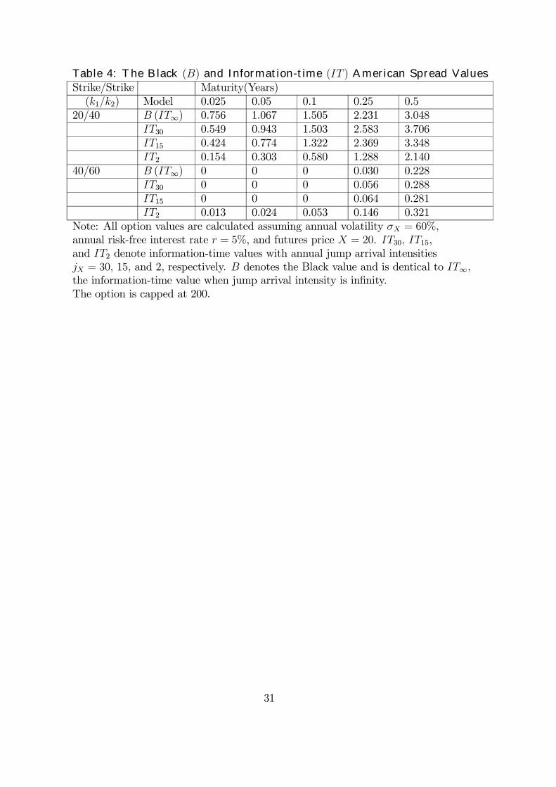
Table 4: The Black (B) and Information-time (IT ) American Spread ValuesStrike/Strike Maturity(Years)(k1/k2) Model 0.025 0.05 0.1 0.25 0.5

20/40 B (IT∞) 0.756 1.067 1.505 2.231 3.048IT30 0.549 0.943 1.503 2.583 3.706IT15 0.424 0.774 1.322 2.369 3.348IT2 0.154 0.303 0.580 1.288 2.140

40/60 B (IT∞) 0 0 0 0.030 0.228IT30 0 0 0 0.056 0.288IT15 0 0 0 0.064 0.281IT2 0.013 0.024 0.053 0.146 0.321

Note: All option values are calculated assuming annual volatility σX = 60%,annual risk-free interest rate r = 5%, and futures price X = 20. IT30, IT15,and IT2 denote information-time values with annual jump arrival intensitiesjX = 30, 15, and 2, respectively. B denotes the Black value and is dentical to IT∞,the information-time value when jump arrival intensity is infinity.The option is capped at 200.

31

Table 5: Values of Reinsurance Contracts (ROL)with CAT Bonds and Basis Risk

KCATbond 80 100 120ρc 0.3 0.5 1 0.3 0.5 1 0.3 0.5 1

(λ, σc, σcindex) ARe/DRe=1.1(0.5,0.5,0.5) 0.00283 0.00283 0.00283 0.00283 0.00283 0.00283 0.00283 0.00283 0.00283(0.5,1,1) 0.01696 0.01698 0.01709 0.01694 0.01695 0.01701 0.01694 0.01695 0.01701(0.5,2,2) 0.05335 0.05354 0.05424 0.05327 0.05343 0.05403 0.05326 0.05340 0.05392(1,0.5,0.5) 0.01067 0.01067 0.01607 0.01066 0.01066 0.01066 0.01066 0.01066 0.01066(1,1,1) 0.03989 0.03995 0.04018 0.03987 0.03990 0.04002 0.03978 0.03978 0.03986(1,2,2) 0.10632 0.10663 0.10798 0.10615 0.10640 0.10749 0.10594 0.10620 0.10712(2,0.5,0.5) 0.04331 0.04331 0.04337 0.04331 0.04331 0.04333 0.04331 0.04331 0.04331(2,1,1) 0.09952 0.09964 0.10011 0.09931 0.09938 0.09967 0.09925 0.09930 0.09943(2,2,2) 0.21774 0.21825 0.22703 0.21719 0.21767 0.21981 0.21687 0.21732 0.21910

ARe/DRe=1.3(0.5,0.5,0.5) 0.00296 0.00296 0.00296 0.00295 0.00295 0.00295 0.00295 0.00295 0.00295(0.5,1,1) 0.01904 0.01905 0.01918 0.01902 0.01902 0.01908 0.01902 0.01902 0.01906(0.5,2,2) 0.06184 0.06203 0.06280 0.06177 0.06193 0.06259 0.06175 0.06189 0.06246(1,0.5,0.5) 0.01123 0.01123 0.01123 0.01123 0.01123 0.01123 0.01123 0.01123 0.01123(1,1,1) 0.04479 0.04484 0.04510 0.04492 0.04494 0.04508 0.04473 0.04473 0.04482(1,2,2) 0.12335 0.12365 0.12512 0.12342 0.12367 0.12488 0.12300 0.12326 0.12428

(2,0.5,0.5) 0.04669 0.04669 0.04670 0.04666 0.04666 0.04667 0.04663 0.04663 0.04663(2,1,1) 0.11265 0.11277 0.11337 0.11249 0.11257 0.11292 0.11237 0.11242 0.11258(2,2,2) 0.24566 0.24603 0.24791 0.24531 0.24567 0.24732 0.24506 0.24540 0.24677

ARe/DRe=1.5(0.5,0.5,0.5) 0.00296 0.00296 0.00296 0.00296 0.00296 0.00295 0.00296 0.00296 0.00296(0.5,1,1) 0.02016 0.02018 0.02030 0.02017 0.02017 0.01906 0.02020 0.02020 0.02023(0.5,2,2) 0.06887 0.06905 0.06988 0.06882 0.06897 0.06246 0.06887 0.06899 0.06962(1,0.5,0.5) 0.01130 0.01130 0.01130 0.01130 0.01130 0.01123 0.01130 0.01130 0.01130(1,1,1) 0.04767 0.04771 0.04800 0.04764 0.04766 0.04482 0.04763 0.04763 0.04773(1,2,2) 0.13795 0.13824 0.13983 0.13796 0.13820 0.12428 0.13768 0.13793 0.13907(2,0.5,0.5) 0.04735 0.04735 0.04735 0.04733 0.04733 0.04663 0.04734 0.04734 0.04734(2,1,1) 0.12066 0.12076 0.12147 0.12051 0.12057 0.11258 0.12055 0.12058 0.12080(2,2,2) 0.27106 0.27153 0.27417 0.27066 0.27110 0.24677 0.27038 0.27081 0.27268Note: This table presents ROLs with CAT bond issuance and the payoffs to CATbonds are linked to a catastrophe loss index. ROLs are calculated and reportalternative sets of trigger values (KCATbond), catastrophe intensities (λ), catastrophe lossunder volatilities (σc, σcindex) and the coefficient of correlation between the reinsurer’scatastrophe loss and the composite loss index (ρX). ARe/D represents the initialasset-liability structure or capital position of the reinsurers.All estimates are computed using 20,000 simulation runs.

32