tax-deductible pre-event catastrophe loss … pre-event catastrophe loss reserves: the case of...

Milidonis and Grace (2008): Catastrophe Reserves

Tax-Deductible Pre-Event Catastrophe Loss Reserves: The Case of Florida1,2

By

Andreas Milidonis3, Ph.D. Martin F. Grace Ph.D., JD

James S. Kemper Professor of Risk Management Department of Risk Management & Insurance, Robinson College of Business, Georgia State University, Atlanta, GA, 30303, USA. Tel: +1 404 413-7469; Email: [email protected]

Accounting and Finance Division, Manchester Business School, University of Manchester, Crawford House, Booth Street East, Manchester, M13 9PL, U.K. Tel: +44(0)161-275-3936 Email: [email protected]

August 21, 2007

Abstract After Hurricane Andrew the U.S. Congress entertained proposals to allow insurers to

employ tax-deferred loss reserves. Interest was strong at first, but as the events receded interest waned. However, after the most recent severe hurricane seasons the proposals are again being discussed. In this paper we examine the institution of catastrophic loss reserves in a stylized model of insurance provisions. First, we find that the benefits of the tax-deferred loss reserves depend on the actuarial assumptions regarding the expected loss distribution. Second, we make the first attempt at estimating the change in consumer behavior and the social welfare implications for permitting tax deferred loss reserves. In sum, we find under specific circumstances there are large welfare gains for allowing the tax deferral of reserves.

Keywords Tax-Deferred Loss Reserve; Catastrophe Financing and Pricing; Extreme Value Theory; Mixture model; Insurance; Reinsurance; 1 This paper will appear ASTIN Bulletin volume 38.1. 2 We would like to thank Sam Cox for suggestions on actuarial methodology. We would also like to thank Richard Derrig, Richard Phillips and Tyler Leverty for comments and assistance on an earlier version of the paper and further acknowledge the prompt and valuable help of Mr. Edward N. Trevelyan of the U.S. Census Bureau. Finally, we would like to thank an anonymous referee for his/her insightful comments. All errors or omissions, however, are the authors’ responsibility. 3 Contact Author.

mailto:[email protected]

mailto:[email protected]


1. INTRODUCTION The dramatic increase in catastrophic losses in the 1990s forced property-liability insurers to recognize the potential to incur losses of a magnitude not previously experienced. Several developments have taken place in the market since then including the development of catastrophe bonds, the continued refinement and implementation of catastrophe simulation models using detailed trends in climatological data as predictors for catastrophes, and the introduction of public sector schemes designed to provide protection to private insurers for the most extreme losses. An example of one such program which did not materialize was a proposal by the Clinton Administration which would have provided high layer excess-of-loss reinsurance to the private insurance industry underwritten by the U.S. Treasury (Lewis and Murdock, 1996).

Another example is the proposed establishment of tax-deferred pre-event catastrophe reserves. This proposal would allow private insurers and reinsurers to set up reserves which could only be assessed in the case of a catastrophe (Davidson, 1996). Such reserves have long been employed by insurance companies in Europe, Japan and Puerto Rico. This essentially puts US insurance and reinsurance companies at a disadvantage internationally since their competitors are not called to pay taxes on investment income from these reserves.

According to the financial pricing literature the price of insurance depends on expected future losses, the cost of equity capital and the insolvency put reflecting each company’s financial position and obligation to meet future claims (Phillips, Cummins and Allen, 1998). In this paper we estimate the part of premiums charged by stock insurers that is attributable to the tax-cost of equity capital. A publicly traded insurance company, like any other financial institution, can be financed either through debt or equity. However, a possible debt renegotiation or bankruptcy of an insurer could permanently tarnish the demand for coverage and alter the insolvency probability of the insurer. For simplicity we consider only one source of capital for the stock insurer: equity capital. More specifically, the stock insurer collects premium from policyholders and equity capital from the market at the beginning of the year. At the end of the year, any claims by policyholders are paid out and any residual amounts are distributed to equity holders.

The cost of equity capital becomes a major part of the price of insurance especially when contracts cover losses occurring from extreme events such as Hurricane Andrew in Florida in 1992 and Hurricane Katrina in 2005, which were the largest ever recorded catastrophes in terms of direct insured losses. Therefore, companies need equity capital to build reserves to enable them to reduce the probability of insolvency from future catastrophic losses. In a competitive environment such as the market for property-casualty insurance, companies cannot absorb the cost arising from equity capital. Therefore they have to pass it onto consumers in order to remain solvent. Consequently homeowners are called to pay more than the actuarial fair value of an insurance contract since they have to absorb part of the total cost of equity capital.

The cost of capital can be anywhere from 11% to more than 1,000% (for larger layers of insurance) of the present value of expected claim costs (actuarial fair value of the underlying risk), thus making insurance potentially unaffordable (Harrington and Niehaus (HN) (2003). Our paper is based upon the potential unwillingness on the part of insurance companies to offer insurance at the actuarial fair value of underlying risks, as well as unwillingness on part of the consumers to pay prices which would be mostly a function of the cost of capital of the insurer. This leads to a shortage of insurance coverage.

- 1 -


Furthermore, the occurrence of new catastrophes results in a decrease in the amount of insurance reserves which, in turn, could increase the number of uninsured homeowners as prices rise. As a result the government is called to release disaster relief funds to cover the alleged social welfare gap that arises from losses suffered by under-insured or uninsured homeowners.

Tax-deferred pre-event catastrophe reserves may provide a partial long term solution to this problem. This is because companies will be able to put reserves aside for which they will not have to pay taxes unless a certain number of years go by without a triggering event.4 Assuming that insurers pass any savings from tax-deferrals on such reserves to consumers, as homeowners’ markets are reasonably competitive, prices are expected to decrease since the cost of equity capital for insurers will decrease.

2. CONTRIBUTIONS

We make four contributions in this paper. First, we estimate the aggregate loss

distribution for insured catastrophic losses for the state of Florida, using a dataset of historical catastrophe losses since 1949 from PCS.5 In order to account for the recent increasing trend in the frequency and severity of hurricanes we estimate the distribution by using the most recent recorded losses (1990-2004). In addition we refine estimates of loss events in the tails of both distributions by using Extreme Value Theory.

Our second contribution is the estimation of the portion of premiums of homeowners’ catastrophic insurance attributable to federal income taxes insurers pay on investment income and eventually pass on to consumers. We do so by evaluating HN’s model over different layers of homeowners insurance against catastrophic damages, using the estimated aggregate loss distribution.

Our third contribution is the calculation of the expected percentage increase in the quantity of homeowners’ catastrophic insurance demanded in Florida. We do this by using estimates of price elasticity of homeowners’ demand estimated by Grace, Klein, and Kleindorfer (GKK) (2004).

Our last contribution is the estimation of the social welfare effects of this proposal. Assuming a horizontal supply curve, where all savings from the proposal will eventually be passed onto the consumer, we estimate the loss in federal tax revenue and the social welfare gain to the consumers in Florida by allowing the establishment of pre-event tax-deferred catastrophe reserves. Finally we calculate the federal assistance funds released to uninsured homeowners’ losses in Florida resulting from catastrophes and compare them with projected social welfare gains from the tax-deferred proposal.

In section 3 we explain the rationale for using the last fifteen years of data to estimate the aggregate loss catastrophic distribution to evaluate our model, in section 4 we describe the data and in section 5 we discuss the model and its implications. Section 6 describes the actuarial methodology used to estimate the aggregate loss distributions. In Section 7 we state our economic assumptions and discuss the economic implications of

4 The recent proposed legislation suggests a twenty-year time frame under which companies can accumulate funds tax-free, at the end of which period they have to release parts of those funds as taxable revenue, unless of course a catastrophe takes place that depletes these reserves. Funds from such reserves will be used only if losses exceed a pre-determined loss based proportionally on the risk that each company undertakes. 5 PCS stands for Property Claims Services, a unit of ISO, based in New Jersey.

- 2 -


enacting the proposal while in section 8 we estimate the social welfare effects. We conclude in section 9.

3. CHANGES IN HURRICANE FREQUENCY AND SEVERITY DISTRIBUTIONS

Over the past decade we witnessed more intense hurricanes in the North Atlantic

basin. The 2005 hurricane season has broken many of the previous records set in terms of both human and financial cost. Hurricane Katrina which struck Louisiana, Mississippi and Alabama was responsible for about 1,300 hundred deaths and had insured damages of about $35 billion dollars. It is now ranked third on the list of deadliest and first on the list of costliest hurricanes to hit the US (Blake, Rappaport, Jarrell and Landsea, 2005). Wilma, another hurricane in 2005, which struck south Florida, has also captured the first place among the most intense hurricanes with a record pressure of 822 millibars.

A growing literature is developing among oceanologists and weather researchers which documents and attempts to explain the variation in trends in hurricane activity. Webster et.al. (2005) find evidence of an increasing trend in hurricane frequency and intensity in the North Atlantic basin over the last decade. On another note, Emanuel (2005) uses an index of potential destructiveness of hurricanes and finds that hurricanes have become potentially more destructive today compared to the 1970s. In an earlier article, Gray (1990) finds a strong association between West African rainfall and US landfall of intense hurricanes. More specifically the author examines drought periods in West Africa and hurricane intensity in the North Atlantic basin. In his paper he forecasts that a higher number of intense hurricanes should be expected to make landfall in the US and Caribbean basin from 1990 through the early years of the 21st century. More recent research (Goldenberg, Landsea, Mestas-Nunez & Gray, 2001) support Gray’s predictions and further note that if the era of increased hurricane activity that started in 1995 continues, we should expect to see more intense hurricanes making landfall in the Caribbean and US in the next few decades.

As was expected, several public policy proposals were suggested to improve on how the government can help insurers prepare for future expected losses from catastrophes. One of these suggestions envisions permitting insurers to establish pre-event tax deductible catastrophe loss reserves, so that insurers can supply homeowners’ insurance at lower prices. These lower prices come from the estimated savings insurers will have from not paying federal taxes on investment income. The proposal suggests that federal taxes on investment income will have to be paid by insurers only in the case that a major catastrophe does not hit the US for an extended period of time. Alternatives to the tax-deferred proposal include establishing a National Disaster Insurance corporation, a government reinsurance program and state insurance funds (see e.g., Grace and Klein, 2002).

Our paper extends prior discussions on the pricing of tax-deferred catastrophe reserves (Harrington and Niehaus 2001, 2003) by providing a range of expected changes in the price and quantity demanded of catastrophic insurance as well as the social welfare implications from establishing these reserves. In order to provide realistic estimates of this forward looking proposal, we test our results using two distributions for the expected aggregate losses from catastrophes. Our first simulated distribution is derived using a dataset of insured catastrophe losses from 1949-2004 while the second simulated distribution is using the same dataset but only for losses after 1990. We decided to use these two distributions in order to capture the changing increasing trend in hurricane frequency and severity that we have been experiencing since the early 1990s. For brevity reasons we only

- 3 -


report the results obtained by evaluating the most recent distribution, while both sets of results can be found in an earlier version of this paper (Milidonis and Grace, 2007).

4. DATA

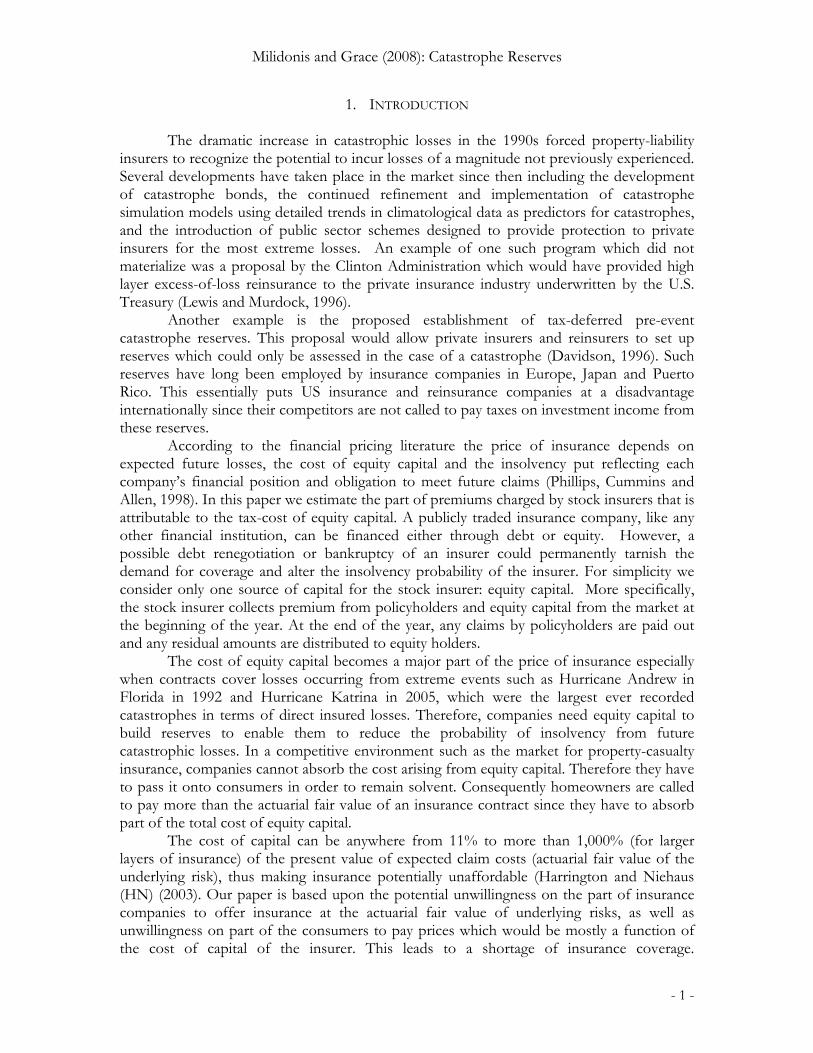
The first data set used for this paper was obtained from Property Claim Services (PCS) and contains historical insured catastrophic losses that have taken place in Florida since 1949. PCS collects data from a network of agents and other sources throughout the US about losses resulting from disasters in the US since 1949. A disaster is categorized as a catastrophe if it exceeded $1 million before 1983, $5 million from 1983 to 2004 and $25 million after 2004.6 During the 56-year span (1949-2004), 125 disaster-related insured losses were recorded by PCS. Furthermore, there were significant changes in the value of the underlying property insured under homeowners’ insurance contracts. In order to account for changes in the insured property value and economic inflation, we constructed a Housing Value Index (HVI) for the state of Florida in order to make all loss amounts since 1949 equivalent to 2004 dollar values. For the HVI we have gathered the value of specified7 owner-occupied housing as reported by the U.S. Census Bureau (reported in ten year intervals back to 19508) and normalized housing values against the 2004 housing values to get annual accumulation factors for all years since 1949.9

Catastrophe Count Mean Standard Deviation Median Kurtosis Skewness Minimum MaximumBrush fires 2 39,279,511 41,862,809 39,279,511 - - 9,678,035 68,880,988 Hurricanes 28 1,755,301,407 4,568,428,604 203,167,540 19 4 601,407 23,160,673,653 Tornadoes 9 42,629,985 41,883,154 26,670,679 1 1 5,691,685 130,908,748 Wind 84 44,366,875 138,777,044 13,845,632 35 6 1,086,950 920,962,197 Other 2 94,861,714 121,006,492 94,861,714 - - 9,297,202 180,426,225 TOTAL 125 428,217,673 2,251,675,582 20,203,199 86 9 601,407 23,160,673,653

Table 1(i): Descriptive Statistics: Florida Property Catastrophes (1949-2004)

NOTE: Losses were adjusted to 2004 exposure and price levels using the Housing Value Index.SOURCE: Property Claims Services

Catastrophe Count Mean Standard Deviation Median Kurtosis Skewness Minimum MaximumBrush fires - - - - - - - - Hurricanes 10 4,579,136,901 6,982,381,467 2,490,809,849 7 2 60,491,284 23,160,673,653 Tornadoes 8 41,135,009 44,517,528 24,068,510 1 2 5,691,685 130,908,748 Wind 41 75,505,579 194,284,196 19,343,693 16 4 1,676,360 920,962,197 Other - - - - - - - - TOTAL 59 834,172,505 3,240,859,911 26,670,679 40 6 1,676,360 23,160,673,653

NOTE: Losses were adjusted to 2004 exposure and price levels using the Housing Value Index.

Table 1(ii): Descriptive Statistics: Florida Property Catastrophes (1990-2004)

SOURCE: Property Claims Services

6 The thresholds used in the data pertain to the total losses incurred from one event. In our case we focus our analysis only on the state of Florida (due to limitations in price elasticity estimates of homeowners insurance in Florida only). Therefore, in isolating costs from catastrophes that only involve Florida, there are data points that are below the thresholds specified by PCS. 7 Represents single family units on less than 10 acres without a business or medical office on the property 8 Specified owner occupied housing value was the only value reported consistently back to 1950 in contrast to the Owner-occupied housing value (includes specified owner-occupied value) which was not reported for 1970. 9 The HVI was used to multiply losses that took place in 1949 by a factor of 19.44, in 1950 by 18.28, etc. These factors were determined by dividing the value of specified-owner occupied housing for each year by the value estimated for year 2004. Linear interpolation was used to get housing values for the years between the 10-year periods lapsing between census reports.

- 4 -


Descriptive statistics of all 125 losses are reported in Table 1(i) by type of reported catastrophe. In Table 1(ii) we summarize all recorded losses since 1990. As mentioned above, the most recent data (1990-2004) includes more frequent and severe catastrophes, which are mainly a result of wind damage from increased hurricane activity. Both data sets are very much skewed to the right with the mean of the entire dataset ($428 million, Table 1i) being about 21 times the median ($20 million, Table 1i). In a similar fashion the more recent catastrophes show a similar pattern with the mean ($834 million, Table 1ii) being about 31 times the median ($27 million, Table 1ii).

The difference between the mean and the median of loss amount is attributed to the 28 hurricanes that have taken place over the years with an average loss amount of $1.755 billion (10 hurricanes since 1990 with a mean value of $4.579 billion), while wind losses make up most of the remaining observations. In Figure 1 we have plotted the loss amounts of the 125 catastrophes which took place in Florida in chronological order.

Figure 1: Individual Florida Catastrophic Loss Events(1949-2004)

0

5,000

10,000

15,000

20,000

25,000

20/0

8/19

4920

/08/

1951

20/0

8/19

5320

/08/

1955

20/0

8/19

5720

/08/

1959

20/0

8/19

6120

/08/

1963

20/0

8/19

6520

/08/

1967

20/0

8/19

6920

/08/

1971

20/0

8/19

7320

/08/

1975

20/0

8/19

7720

/08/

1979

20/0

8/19

8120

/08/

1983

20/0

8/19

8520

/08/

1987

20/0

8/19

8920

/08/

1991

20/0

8/19

9320

/08/

1995

20/0

8/19

9720

/08/

1999

20/0

8/20

0120

/08/

2003

LO

SS (

$MIL

LIO

N)

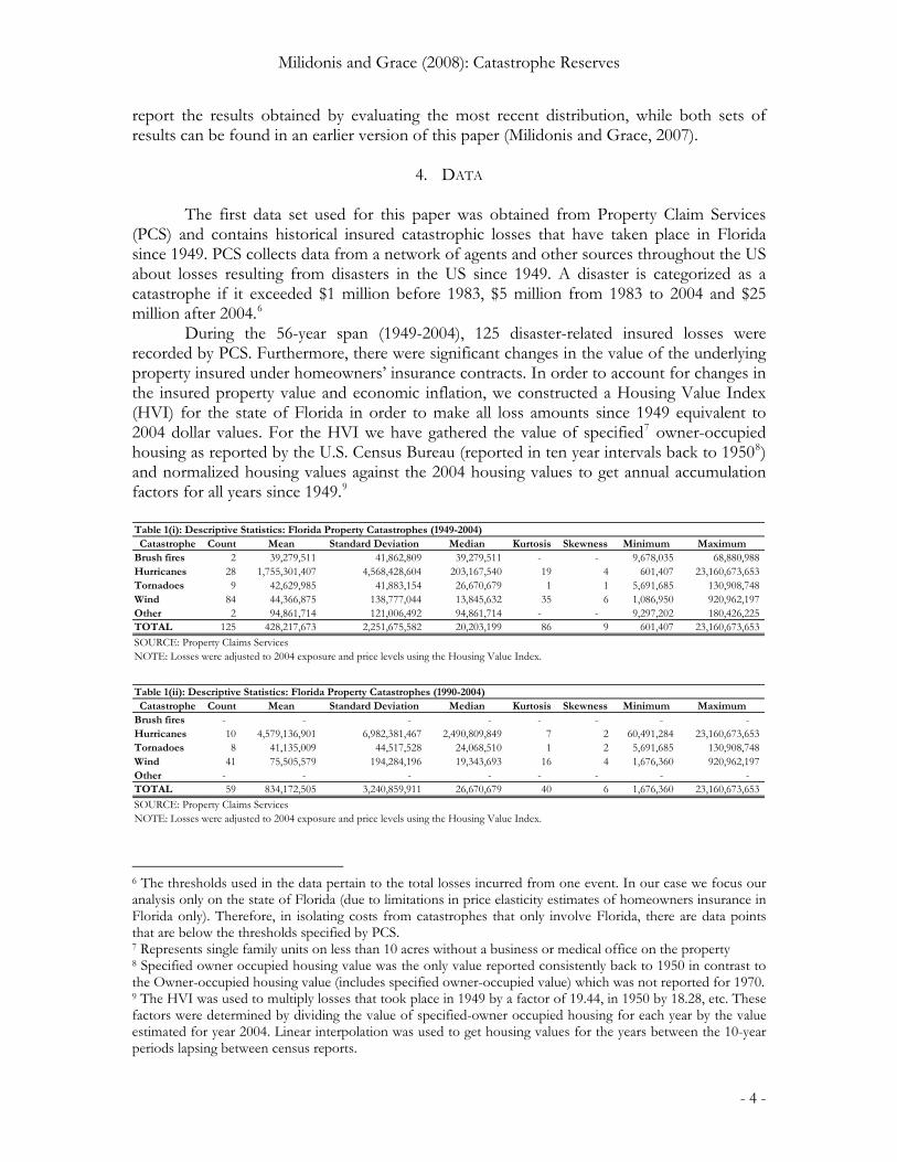
It is obvious from the chart that Hurricane Andrew surpasses all other losses since the second ranked event was Hurricane Charley in 2004 which was about three times smaller in insured damages than Andrew ($7.4 billion vs. $22.3 billion). Another important observation is that in 2004 we had 4 hurricanes landing in Florida with estimated total insured losses of $19 billion. As far as the frequency of catastrophes in Florida is concerned, Figure 2 shows their trend since 1949. From the graph we can see that besides 1949 and 1950, catastrophes were almost non-existent until 1963. At that point and until 1977, up to three events per year were recorded while after 1978 there was a variable trend ranging from zero to eight until the early nineties. Finally, we observe that at least two catastrophes per year were recorded over the

- 5 -


last fifteen years, which we used as the basis of our estimated distribution that captures this increasing trend.10 In the last part of our paper we use a dataset of Federal Disaster Assistance funds released from 1983-2001 to compare the projected social welfare benefits of the tax-deferred proposal with the money spent by the Federal government to remedy the losses of uninsured homeowners. This dataset includes grant outlays and obligations to the state of Florida, local governments and other individual recipients. The data had to be carefully parsed in order to isolate the part of disaster assistance dollars that were given to uninsured homeowners. This was because there were frequent changes in program codes over the years and also due to the fact that much money was spent in other tasks like cleaning debris and fixing public

Figure 2: Annual Frequency of Florida Catastrophic Events(1949-2004)

0

2

4

6

8

10

1949

1951

1953

1955

1957

1959

1961

1963

1965

1967

1969

1971

1973

1975

1977

1979

1981

1983

1985

1987

1989

1991

1993

1995

1997

1999

2001

2003

Num

ber o

f Eve

nts

transportation and utilities. However we believe that our approach to take into account only the money that would not have to be spent in a future catastrophe if people could have afforded catastrophic home insurance, gives us an accurate estimate of the amount of Federal assistance dollars used for our analysis.11 All details on the programs that we used in our analysis as well as the money given out for each program for the period 1983-2001 are summarized in section 8 and Table 14.

5. MODEL 5.1 Harrington & Niehaus (2003)

10 Details of estimating the frequency and severity distributions are given in section 6(a) and 6(b). 11 As in the case of catastrophes, all amounts were multiplied by the HVI factors in order to bring everything to 2004 US dollars. We only include funds released up to 2001 since there is usually a time-lag between when a disaster hits and when the entire disaster funds pertaining to a catastrophe are released. The data set was obtained from the Census Bureau website.

- 6 -


The tax-deferred proposal suggests a way that insurance companies will be able to set up reserves in such a way that can reduce prices to consumers. According to the financial economics literature, the price of insurance consists of the present value of expected losses, a part attributable to the cost of equity capital and a premium that companies in good financial standing charge because they can provide more security to the consumer that their claims will be paid out (Cummins, 1990; Phillips, Cummins and Allen, 1998; Myers and Cohn 1987). This proposal aims at decreasing the “cost of equity capital” part of the price by deferring taxes on investment income payable to the federal government In order to derive a first estimate of the cost of capital as a percentage of the price of insurance we use the Harrington and Niehaus (HN) one period model. In their model HN solve two simultaneous equations to estimate the premium (P) and capital (K) that insurance companies would need in order to stay in business in the case of a catastrophe. The first equation (equation 1: capital market constraint) equates the accumulated value of equity capital based on the market’s required rate of return (left hand side) with the expected payoff function of the insurer as that is determined by the distribution of aggregate catastrophic losses, the corporate tax structure and the company’s payoff function. The second equation (equation 2: insolvency constraint) assigns an exogenous insolvency probability which has to be less than or equal to the ratio of expected unpaid claims divided by total expected insured losses.

( ) ( ) ( )( )

( )( )

( )( )( )11

1

13

1

20

1 dLLfdLLfdLLfrKrKP

KrrP

KrrP

∫∫∫+++

+++

+++

Π+Π+Π=+α

α

α

α

α

( )( )[ ] ( )( )( )

( ) ( ) ( )

( )( )[ ] ( )

( ) ( ) ( )( )2

111

dLLfdLLfL

dLLfrPK

dLLfdLLfL

dLLfrPKLrPK

∫∫

∫

∫∫

∫∞

+

+

∞

+∞

+

+

+

+++

+−

++−+

+−

−++−

=

λα

λα

α

λα

λα

λα

α

λα

α

λα

λ

λα

αγ

The values of the two unknowns, premium (P) and capital (K), are obtained by solving the capital market and insolvency equations simultaneously. Values for P and K are obtained for several exogenously given parameters.

The basic scenario calculates the premium (P) that an insurer has to charge and the amount of capital (K) it has to collect from equity holders in order to offer a contract for a layer of insurance ( λ ) over an attachment point (α ) against catastrophic losses (L). The distribution represents the probability density function of aggregate catastrophic losses in the state of Florida. This is estimated by fitting a mixture aggregate loss model (section 6c) on simulated data from frequency and severity distributions that will be estimated from the PCS dataset on historical catastrophic losses. Since we are aggregating losses to the industry level, the model assumes that there exists only one insurance (reinsurance) company in Florida that offers insurance (reinsurance) contracts at competitive prices (P) as those are determined by the solution to the two simultaneous equations above. The theoretical justification for our assumption is that it is Pareto optimal for each insurer to hold a proportion of the “market portfolio” of insurance contracts whereby each insurer pays a portion of total industry losses (Borch, 1962). Therefore the industry behaves as a single firm which pays 100% of the losses up to the point that net premiums and equity capital run out.

( )Lf

- 7 -


The capital market constraint (equation 1) integrates the insurer’s payoff12 function (right hand side) over the three integral limits and sets it equal to the capital at the end of the period which is accumulated by the market risk-free interest rate (r). denotes the insurer’s payoff for each of the three integrals which varies according to losses, L, that are expected to occur. The following example explains how the model works.

iΠ

Assuming that we have one insurance company offering homeowners catastrophic insurance coverage at competitive prices over one time period, then this company needs to calculate what premium (P) to charge to homeowners and the amount of equity capital (K) it will need. At the end of the period, K with the market required return, K*(r), and any residual profits (∑ ) will have to be returned to equity holders. To determine profits we

deduct expected claims (a function of L), from revenues (Premiums and Investment return on Premium and Capital). Expected claims are calculated by evaluating the distribution of annual aggregate loss claims, , over the entire range of losses the insurer will cover.

Πi

i

( )LfThe important implication of the HN model is that the insurance company has to

pay corporate taxes on its underwriting revenue, ( )rP +1 , and investment income, ( )rK , when taxable earnings are positive. The part of the insurance price attributable to the cost of equity capital pertains to the taxes the company has to pay on K when taxable earnings are positive. However in the case that taxable earnings are depleted, the company receives a tax-reimbursement equal to τ*b provided it remains solvent where b is the value of tax shields that takes a value between zero and one and τ the corporate tax rate. If the insurer becomes insolvent, while it still has indemnity obligations to policyholders then the company has no tax shields. This non-linear corporate tax schedule makes the payoff structure also non-linear. As a result the company has different payoffs over different ranges of losses (equation 1), which we explain below.

12 Harrington and Niehaus (2003) provide detailed explanations and diagrams regarding the corporate tax structure and company payoff functions used in equations 1 and 2. In short, since the corporate tax structure is non-linear (due to tax shields given to companies when they make a loss), the payoff function of the company is also non-linear. In addition the payoff function depends on which funds are used first to pay off claims. According to the model investment income from premiums and capital is used first while actual reserves from capital are used second.

- 8 -


Figure 3 shows the structure of the proposed contract which forms the basis for the model. The insurer offers coverage for a layer of insurance, λ , over an attachment point α . Since losses (claims) are stochastic, they can fall anywhere along the x-axis of Figure 3. In the first case, if losses fall to the left of α the company does not have to pay any losses to policyholders and at the end of the year it pays out profits to shareholders equal to the sum of all premiums collected, the investment return on premiums minus corporate taxes on premiums and investment income. All equity capital (in addition to the investment income on capital, minus corporate taxes) is also returned to the market. We calculate by subtracting taxes from taxable revenues for the insurance company

1Π

( )( ) ( )( )1 1 1 ; 0K P r P r Kr Lτ αΠ = + + − + + ≤ <⎡ ⎤⎣ ⎦ .

In order to calculate we examine the case that losses fall to the right of alpha, to the left of

2Πλ and below the maximum taxable revenues, ( ) KrrP ++1 . In this case only

losses in excess of α are paid out. Taxes are only paid on the taxable revenues. Therefore would be the amount of taxable revenues remaining after losses and taxes are paid out 2Π

( )( ) ( ) ( ) ( )[ ] ( )( )KrrPLLKrrPLrPK +++<≤−−++−−−++=Π 1;112 ααατα . The next possible range of losses, 3Π , would be again between α and λα + but in

excess of maximum taxable revenue and below the maximum losses that the insurer can13 pay, ( ) ( rKP +++ 1* )α . In this case the insurer will pay losses in excess of α (as before), but since it will have to draw on capital to make loss payments, the insurance experiences a loss and no corporate taxes will be paid. Instead tax shields will be provided by the government. We follow HN2003 notation and use b 14 to denote the value of tax shields. Tax shields will be paid only on the amount of capital that the insurer will have to use to cover losses. Therefore, there will be no amount left to be given to equity holders at the end of the period ( )( ) ( ) ([ ) ( ) ]( ;113 rKrPLbrPK −+−LΠ = + + − − +τ −αα

( ) +<≤+++ αα LKrrP 1 ( )( ))rKP ++ 1 . Finally, if the firm is insolvent 4Π will be zero since losses will be in excess of

λα + , in which case the insurer will become insolvent as premiums, capital and investment income will fall short of the total promised claims ( λ ).

The second equation (equation 2) addresses the solvency issue of the insurance company, a necessary condition for the insurance company to meet the capital market constraint. The left hand side of the insolvency constraint states the probability of insolvency (γ ) while the right hand side represents the ratio of expected unpaid claims divided by the total expected promised claims. Expected unpaid claims (numerator of left hand side) are a function of the aggregate loss density function, the order to claim payment, the required market return and the level and attachment point of insurance, while the total expected claims represent the loss exposure of the insurance company as those are stated by the contract terms. The insolvency probability is given as an exogenous variable.

13 The sum of premiums, capital and investment income of the insurer is equal to ( ) λγ *1− , which is equal to the probability of staying solvent times total promised claims. 14 “b ” takes values between 0 and 1 to account for the time taken to collect tax shields. For example a value of 1 means that the company will receive all tax shields at the end of the year, while values less than 1 means that it will take a few years for tax shields to be received and they are therefore discounted.

- 9 -


Given that we have to simultaneously solve equations 1 and 2 to get values of P and K, we now turn to the methodology that we use to estimate the aggregate loss distribution for insured catastrophic losses in Florida, ( )Lf .

5.2 The Aggregate Loss Model

Klugman, Panjer and Willmot15 (1994) have a collection of aggregate loss models which can be used to estimate the annual aggregate catastrophic loss distribution. From equation 3 below the aggregate loss random variable, , is determined for year t as the sum of independent and identically distributed losses, , where both the number of losses,

, and the value of each individual loss amount, , are independently generated from the estimated frequency and severity distributions.

SN jX

N jX

,.....21 ntttjt XXXS +++= Nj ...,2,1= ; 000,25...,2,1=t (3) Using maximum likelihood estimation and several goodness-of-fit tests, the best frequency and severity distributions are chosen from a number of different distributions that are fit on the historical data set. Using the selected frequency and severity distributions, we then simulate the number of annual losses for 25,000 years and then the severity of each loss using the estimated severity distribution. Then individual losses within one year (sum of within a year t ) are summed together to get an annual aggregate loss amount, . We repeat this procedure 25,000 times in order to obtain a vector of (

jtX

jtS

tS 000,25...,2,1=t ). Maximum likelihood estimation is then used to estimate the best probability density function, . ( )Lf

6. METHODOLOGY 6.1 The Frequency distribution

The first step in deriving the aggregate loss distribution is to estimate the frequency at which catastrophes take place in the state of Florida every year. From 1990 to 2004, 59 catastrophes were recorded by PCS for the state of Florida. From a total of 15 annual observations we observe that at least two events took place every year, while interestingly enough, one year had seven events (Figure 4).

KPW explain that in choosing a frequency model, the sample mean and variance provide an indication of which distribution to use out of the three main candidates: Poisson, Negative Binomial and Binomial distributions. More specifically they state that if the sample variance is larger than the sample mean then this is an indication that the Negative Binomial distribution may be a good fit. In the case that the sample mean exceeds sample variance then the Binomial distribution will probably fit the data best while in the case the sample mean and variance are the same then the Poisson distribution will probably provide the best fit16. Comparing only the mean and variance (3.93 vs. 2.64; Table 3) of the empirical distribution may be deceiving since the Binomial would be the best candidate.

15 Henceforth KPW. 16 This is because the mean and variance of the three distributions display a different pattern: The Binomial has a larger mean than variance, for the Poisson they are the same and for the Negative Binomial the mean is less than the variance.

- 10 -


Figure 4: Fitting of Frequency Distributions on Annual Catastrophic Losses in Florida (1990-2004)

0

1

2

3

4

5

6

0 1 2 3 4 5 6 7 8+Number of Events per year

Number of Years Poisson Fit Binomial Fit

Events Observedper year Poisson Binomial Poisson Fit Binomial Fit Number of Years

0 0.02 0.01 0.29 0.10 01 0.08 0.04 1.16 0.66 02 0.15 0.13 2.27 1.92 53 0.20 0.22 2.98 3.31 04 0.20 0.25 2.93 3.76 45 0.15 0.19 2.30 2.92 46 0.10 0.11 1.51 1.58 17 0.06 0.04 0.85 0.59 1

8+ 0.05 0.01 0.71 0.16 0Check 1.00 1.00 15.00 15.00 15

Table 2: Frequency Distribution Fits (1990-2004)Probability Expected number

Details Mean Variance LLEmpirical 3.9333 2.6381 Poisson 3.9333 3.9333 (28.63) Binomial 3.9333 2.3862 (27.86)

Null " Poisson is appropriate "Alternative " Binomial is appropriate "Test statistic 1.55Critical (1df, 5%) 3.84P-value 0.21 (CANNOT REJECT)

Table 3: Likelihood Ratio Test for Frequency Distributions (1990-2004)

Using maximum likelihood estimation we fit the candidate models and plot them next to the empirical frequency distribution (Table 2; Figure 4). The frequency plot does not

- 11 -


give us any clear indication whether to pick the Poisson over the Binomial distribution, therefore we employee the Chi-square and Likelihood ratio tests to test their goodness of fit.

The likelihood ratio test (Table 3) does not show a significant difference in log-likelihood values by removing one degree of freedom (using Binomial over Poisson) and therefore does not allow us to reject the Null (Poisson is appropriate). The Chi-square test (Table 4) supports the Likelihood ratio conclusion, that is, the Binomial is rejected as a good fit to the data while the Poisson is not. Therefore, the Poisson distribution ( λ =3.933) is chosen as the frequency model for our data.

Events Observedper Year Poisson Binomial Values Poisson Binomial

- 0.29 0.10 - 0.29 0.10 1.00 1.16 0.66 - 1.16 0.66 2.00 2.27 1.92 5.00 3.28 4.96 3.00 2.98 3.31 - 2.98 3.31 4.00 2.93 3.76 4.00 0.39 0.02 5.00 5.37 5.25 6.00 0.07 0.11

Sum 15.00 15.00 15.00 8.17 9.16

Table 4: Chi-Square Goodness of Fit Test (1990-2004)Expected Values Chi Square Values

Poisson BinomialDegrees of Freedom 4.000 3.000 Confidence Interval 5% 5%Chi - Critical 9.488 7.815 Chi-Square 8.169 9.156 P-Value 8.56% 2.73%RESULT (CANNOT REJECT) (REJECT)

Chi-Square Test Results

6.2 The Severity distribution

The second necessary step before estimating the aggregate loss distribution is to estimate the severity of individual losses taking place at any point in time. As shown earlier, 59 losses have taken place over a period of 15 years therefore adjustments had to be made using the HVI to bring all loss amounts to 2004 US dollars.

After all adjustments we can observe that an event like Hurricane Andrew (which was the most expensive catastrophe in direct insured losses in Florida until 2004), cannot be considered an outlier to the data. Even though other forward looking factors should be incorporated into such models (documented increased trends in frequency and intensity of hurricanes), events in the tail of the distribution should not be ignored.

In choosing the best model for the two datasets we started with five distributions: the Lognormal, Pareto (two-parameter), Exponential, Weibull and Burr12. In figures 5 and 6 the reader can get a first impression of how the candidate models fit the dataset over the entire distribution and the tail, respectively. In order to choose the best distribution for each dataset we use the Kolmogorov-Smirnov (KS) goodness of fit test and then the likelihood ratio test, if applicable, to finalize our choice.

A first indication from the severity plot (Figure 5) is that the two main competitors will be the two-parameter Pareto and the three-parameter Burr12 distribution. The Kolmogorov-Smirnov test confirms that, at all significance levels (Table 5). Finally, the likelihood ratio test rejects the Pareto over the Burr12 distribution since the log-likelihood

- 12 -


value improves significantly by using the distribution with the extra parameter (Table 6). As a result we will use a Burr12 distribution with parameter values: α =2.472709093;

=0.196058179; =6.28060231. In the section below we explain how the aggregate loss distribution is simulated and estimated. q b

Figure 5: Fitting Individual Loss Severity Distributions on the 1990-2004 Dataset

0.00

0.20

0.40

0.60

0.80

1.00

1 10 100 1,000 10,000 100,000LOSS ($MILLION; Log scale)

Empirical BURR 12 PARETO LOGNORMAL WEIBULL EXPONENTIAL

Figure 6: Fitting Individual Loss Severity Distributions on the 1990-2004 Dataset (Tail)

0.80

0.85

0.90

0.95

1.00

100 1,000 10,000 100,000

LOSS ($MILLION; Log scale)

Empirical PARETO LOGNORMAL WEIBULL EXPONENTIAL BURR 12

- 13 -


Confidence Level 90% 95% 99% α β θ μ σ τ qEXPONENTIAL 0.6514 Rejected Rejected Rejected - - 806.22 - - - - PARETO 0.1042 NOT Rejected NOT Rejected NOT Rejected 0.62 - 15.86 - - - - LOGNORMAL 0.1706 Rejected NOT Rejected NOT Rejected - - - 3.79 2.09 - - WEIBULL 0.1945 Rejected Rejected NOT Rejected - - 138.60 - - 0.40 - BURR12 0.0516 NOT Rejected NOT Rejected NOT Rejected 2.47 6.28 - - - - 0.20

Table 5: Fitting of Severity Distributions on Annual Catastrophic Losses in Florida (1990-2004)

*Note: Null Hypothesis is "Distribution Fits the Data well"

Kolmogorov Smirnov* - Critical Values Parameter Estimatesy

DistributionModel

Distribution NLLPareto 346.51Burr12 341.64Null Pareto is appropriateAlternative Burr12 is appropriateTest statistic 9.75Critical (1df, 5%) 3.841P-value 0.76%

(REJECT NULL)

Table 6: Likelihood Ratio Test for Severity Distributions (1990-2004)

6.3 The Aggregate Loss Distribution

The final step before evaluating the two simultaneous equations is to estimate ( )LF . To do that we have to simulate catastrophic events from the frequency and severity distributions estimated above and then estimate the aggregate loss model, , using maximum likelihood one more time. At first we generate 25,000 random annual frequencies from the Poisson (

( )LF

=λ 3.933). For each annual frequency we later generate individual loss events from the Burr12 ( =α 2.427, =q 0.196 and =b 6.281). For each year, individual losses are added together and we finally end up with a vector of 25,000 observations with the total annual cost of simulated catastrophes for each scenario17.

Descriptive Statistics Estimated Distribution based on 1990-2004 data

Probability of loss = $ 0.00 billion 1.90%Probability of loss > $ 0.25 billion 55.95%Probability of loss > $ 0.5 billion 42.73%Probability of loss > $ 1 billion 31.81%Probability of loss > $ 2 billion 23.39%Probability of loss > $ 5 billion 15.47%Probability of loss > $ 10 billion 11.29%Probability of loss > $ 20 billion 8.23%Probability of loss > $ 50 billion 5.42%Probability of loss > $100 billion 3.99%Probability of loss > $200 billion 2.91%

Table 7:Characteristics of the Estimated Florida Annual Aggregate Loss Distribution

Table 7 shows a probabilistic perspective on the simulated dataset by showing the probabilities of a loss exceeding a specified threshold. Interestingly enough, an event of the magnitude of the 1992 losses (includes Hurricane Andrew) or the 2004 losses (includes Hurricanes Charlie, Frances, Ivan and Jeanne etc) which cost about $23 billion and $19 17 In the case that frequency is zero then the annual aggregate losses for that year are zero.

- 14 -


billion respectively, would be expected once in about 12 years. The same event under an estimate of the loss distribution that would be based on the entire 56 years of data rather than the most recent data would be expected to occur once in 333 years (Milidonis and Grace, 2007). This shows the dramatic difference between the most recent years and the full set of data.

In estimating we had to construct a model flexible enough to capture the point mass at zero as well as closely follow the extreme events in the tail. To do that we set up a mixture model (a combination of two or more distributions which do not necessarily form a continuous aggregate model) as follows:

( )SF

( ) ( ) ( )( ) ( )( )[ ] ( )⎪

⎪⎩

⎪⎪⎨

⎧

≥−−+−<≤−+

=<

=

ususHuBppussBpp

sps

sF

σξ ,*1101

0,0,0

(4)

In this model, is the cumulative density function of the mixture model for the simulated data, is the annual aggregate loss random variable,

( )SFS p is the probability mass at

zero, is the continuous distribution that will be used over ( )sB us ≤<0 , and u is a threshold chosen above which we attach the Extreme Value Theory (Generalized Pareto Distribution), , with shape parameter ( usH −σξ , ) ξ and scale parameter σ . It is important to note that our distribution has a point mass at zero, ( ) 00 =B and the Generalized Pareto distribution is used to model losses in excess of threshold u .

In order to calculate , the parameters of the continuous distribution , and the shape and scale parameters for the Generalized Pareto Distribution (GPD), we use maximum likelihood estimation. We complete the process in two steps: first we estimate

p ( )sb

p and for each dataset where ( )sb ( )sb is fit on the entire range of values greater than zero. To do that we use the following negative log-likelihood function:

( ) ( )[ ] ( ){∑=

−+−−=25000

1ln11lnln

ttt pIsbpIL } (5)

where =1 if S is positive and zero otherwise. In order to make sure that the value of p stays between 0 and 1 when employing maximum likelihood estimation, we use the logistic distribution to estimate p, where

tI

λ takes values between ∞− and ∞+ (Yoo, 2003): ( )

)exp(1exp

λλ

+=p (6)

Confidence Level 90% 95% 99% α β θ μ σ τ qEXPONENTIAL n/a Rejected Rejected Rejected - - n/a - - - - PARETO 0.0114 Rejected Rejected Rejected 0.50 - 133.22 - - - - LOGNORMAL n/a Rejected Rejected Rejected - - - 3.79 2.09 - - WEIBULL n/a Rejected Rejected Rejected - - n/a - - n/a - BURR12 0.0030 NOT Rejected NOT Rejected NOT Rejected 1.28 87.76 - - - - 0.36

Table 8: Fitting of Aggregate Loss Distributions on Simulated Catastrophic Losses in Florida (1990-2004)

*Note: Null Hypothesis is "Distribution Fits the Data well"

Kolmogorov Smirnov* - Critical Values Parameter Estimatesy

DistributionModel

As far as is concerned we fit the Exponential, Weibull, Lognormal, Pareto and

Burr12 distributions. Following the same methodology as in the previous section (6b), we ( )sB

- 15 -


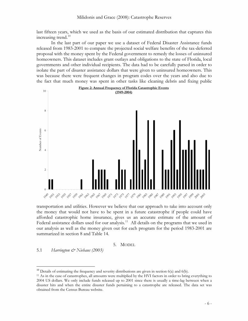
choose Burr12 as the most appropriate distribution for ( )sB ( us <<0 ). As it is expected took the value of the point mass at zero: 0.01896. Furthermore the Burr12 distribution is

chosen as the best model to use for S>0 over the Lognormal and Pareto distributions. Table 8 reports the Kolmogorov - Smirnov test results and parameter estimates of the candidate models which clearly indicates the Burr12 as the best model.

p

6.4 Extreme Value Theory

Even with the Burr12 chosen as the most appropriate model, the tail does not seem to fit the data closely (Figure 7). One alternative to use on the tail of each distribution would be the Extreme Value Theory. It is important to pay attention to the tail of the distribution as the insolvency constraint (equation 2) depends on it. Therefore after picking the Burr12 distribution to estimate losses greater than zero, we then pick a threshold above which we apply the Extreme Value Theory (EVT) to estimate the tail.

Figure 7: Fitting Aggregate Loss Severity Distributions on 1990-2004 Dataset (Tail)

0.9900

0.9920

0.9940

0.9960

0.9980

1.0000

1,000,000 10,000,000 100,000,000 1,000,000,000 10,000,000,000 100,000,000,000 1,000,000,000,000

LOSS ($MILLION; Log scale)

Empirical BURR 12 PARETO

Following McNeil’s (1997) approach we examine high thresholds at the tail of the

distributions, where the EVT would be used, as that is given by the last part of equation 4 ( )( usH −σξ , with support . The distribution we use to apply the theorems of the

EVT is the Generalized Pareto with density function: )us ≥

( ) ( )( )⎪⎩

⎪⎨⎧

=−

≠+−=

−

−

010/*11

/

/1

,ξ

ξσξσ

ξ

σξ ses

sH (7)

where ξ and σ are the shape and scale parameters respectively. Theory suggests that we should estimate the EVT on the excess losses above this threshold. This means that EVT will characterize the part of the mixture model (equation 4) that has observations in excess

- 16 -


of the chosen threshold. In our case the EVT will come into play when we simultaneously solve equations 1 and 2 to get values of P and K that the insurance company will need to have in order to minimize the risk of insolvency18.

The choice of the attachment threshold for EVT is a point of major discussion in the literature. This is because the standard error of the parameter estimates as well as the sensitivity of the Generalized Pareto to the last few data points have to be taken into account in fitting this model. It is important to understand that if the threshold is chosen too low, then the mathematical derivation of the model may no longer be valid, while if the threshold is chosen to be too high, then we might introduce model and parameter uncertainty. (Embrechts, Klüppelberg and Mikosh 1997; McNeil 1997).

Figure 8: Plot of the Generalized Pareto Distribution’s Shape Parameter (ξ) vs. Threshold at Different Levels (1990-2004)

1.50

1.70

1.90

2.10

2.30

2.50

2.70

2.90

0 500 1,000 1,500 2,000 2,500 3,000 3,500 4,000 4,500 5,000

Number of Exceedances at Different Thresholds

Shap

e P

aram

eter

, ξ

In choosing the threshold for ( )sF , we use a combination of methods. Our first

approach is to plot the sample mean excess loss function. This function measures the sample mean above a given threshold and it is characterized by the following equation:

[ uSuSEue >−= |)( ]

(8) In other words, given that some points are above a specified threshold, u , then the mean excess loss function measures the expected value of the difference between the points and the threshold. A plot of this function with respect to different threshold would provide a first indication of whether we have a heavy tail distribution. A straight line plot of )(ue

18 We decided to use the Extreme Value Theory for modeling the tail of ( )sF since the insurance market model we use is evaluated over the entire range of losses. The exogenous insolvency constraint used for equation 2 becomes very much affected by the tail of the distribution. Extreme Value Theory (EVT) is based on the Fischer-Tippet theorem in the same way that the Normal distribution is based on the Central Limit Theorem. This means that EVT is used to model the limiting behavior of the excess of observations above a given threshold, , in the same way that the Normal distribution is used to model the limiting behavior of sums and averages.

u

- 17 -


would indicate the exponential as a likely model19, a downward sloping line would suggest a short-tail, while an upward-sloping line would indicate a heavy-tail distribution. In the case of the GPD the mean excess loss function is linear; therefore we look for points on the plot above which the function behaves linearly with respect to the threshold chosen20.

U (Percentile) U ($Million) Exceedances ξ s80.00% 2,976 4905 2.108 6,525 82.00% 3,768 4415 2.117 8,046 84.00% 4,854 3924 2.126 10,218 86.00% 6,404 3434 2.121 13,664 88.00% 9,029 2943 2.150 18,266 90.00% 13,260 2453 2.177 26,100 91.00% 16,053 2208 2.138 34,486 92.00% 20,779 1962 2.143 44,084 93.00% 28,103 1717 2.182 55,825 94.00% 38,019 1472 2.153 80,904 95.00% 54,609 1227 2.100 127,950 96.00% 90,272 981 2.109 203,258 97.00% 174,453 736 2.164 347,461 98.00% 403,749 491 2.293 719,612 99.00% 1,568,648 246 2.120 4,203,173 99.50% 7,317,572 123 1.973 22,540,579 99.75% 50,134,705 62 2.222 57,414,663 99.90% 188,935,614 25 1.975 589,496,280 99.95% 873,662,722 13 2.262 1,577,254,325 99.98% 4,647,319,460 0 - -

Table 9: Shape parameter values for the Extreme Value Distribution at Different Threshold levels (1990-2004)

The second method we use to pick the thresholds is to plot the value of the shape parameter, ξ , with respect to the threshold chosen (Figure 8). ξ and σ are estimated with maximum likelihood estimation at different values of u (Table 9). The threshold at which ξ showed some stability was consistent with the threshold on the mean excess loss function above which we observed a linear structure. Therefore we picked threshold u equal to 54.609 US$ billion (95th percentile; 1277 exceedances). All parameter estimates are provided in Table 10.

Parameter Distribution based on 1990-2004

p k 1.90%α κ 1.275 q k 0.358 b k 87.761 ξ κ 2.100 σ κ 127,950

uk ($Billion) 54.609uk (Percentile) 95%Exceedances 1277

Table 10: Parameter Estimates of the estimated Mixture model

19 Exponential e(u) = 1/ λ 20 Plots of the mean excess loss function are available by the authors.

- 18 -


- 19 -

Therefore applying the GPD on the tail of ( )sF completes the modeling of the annual aggregate loss distribution which is used in the next section to evaluate the two-equation model. We later project expected decreases in the price of insurance by removing federal taxes on investment income from the model and then estimate increases in the amount of catastrophic homeowners insurance expected from the price decrease. We conclude with a look at the government’s point of view in terms of any savings on federal disaster assistance and any welfare gains.

7 RESULTS 7.1 Base Case and The Effect of Tax-deferral on Price

Using the mixture distribution estimated from section 6, we evaluate the model for many different scenarios in an attempt to capture possible market conditions. The results could equally apply to two cases: either the Florida market can be captured by only one insurance company that provides insurance to homeowners, or there is only one reinsurance company that provides coverage to all insurance companies in Florida. In table 11 we set the background for our analysis. Following the notation in equations 1 and 2, we pick an attachment point α (column 1) and a layer of insurance λ (column 2). Continuing on the first row of Table 11, we then exogenously assign values for the probability of insolvency γ (column 3; 4%), the corporate tax rate τ (column 4; 25%), the value of tax shields21, (column 5; 1.0) and the required rate of return b r (column 6; 6%). For Table 11 we keep γ , τ , b and r constant and we vary α and λ . We start from a contract that covers the first $500 million of industry insured losses and then we successively repeat calculation for the next $500 million layer. In order to examine the effect that extreme losses would have on contracts with large exposures we have designed four contracts (last four rows) in a way that the insurance company covers a larger layer of exposure with no deductible. By solving equations 1 and 2 simultaneously we then calculate the amount of premium P the insurance company has to collect from policyholders (column 8) and the amount of capital K it needs to collect from equity holders (column 9). In column 7 we calculate the present value of expected claim costs (PVECC) which is equal to the total promised claims22 times the probability of staying solvent ( )γ−1

. Since tax costs are the only loading on the PVECC (no administrative expenses included in the model) then the difference between P and PVECC is the tax cost of equity capital. This mark-up from PVECC to P is shown in column 10 and represents the price of insurance; the minimum price above the PVECC that insurance companies charge in order to take on the risk.

The tax-deferred proposal aims at effectively removing this tax “burden” from the pricing formula. Current US tax law does not allow insurers to set up reserves ex-ante that will be used to pay for future losses from catastrophes. Statistically speaking, when insurers collect premiums and equity capital to cover a layer of insurance over a certain period, they should be able to pay all claims within that layer of insurance if their probability of insolvency is zero. However, taxing insurers in years with positive earnings decreases the

21 The tax shields represent the reduction in the value of tax returns the company would receive by carrying forward to future years operating losses (if this was a multi-year model). If the company becomes insolvent however there is no value to tax shields (b=0). 22 The denominator of equation 2.


(1)Attachment

Point

(2)Alpha +

layer

(3)Insolvency constraint

(4)Tax Rate

(5)Value of unused

tax

(6)Interest

Rate

(7)Present Value of Expected

Claim Costs

(8)Premium

(9)Capital

(10)Mark-up


Claim Costs

(12)Premium

(13)Capital

(14)Mark-up

(α) (α+λ) (γ) (τ) (b) (r) (PVECC) (P) (K) (PVECC) (P) (K) Δ Price- 500 4.00% 25% 1.00 6.00% 273.886 297.075 148.226 8.47% 273.886 273.886 171.415 - -8.47%500 1,000 4.00% 25% 1.00 6.00% 164.958 195.497 254.700 18.51% 164.958 164.958 285.239 - -18.51%

1,000 1,500 4.00% 25% 1.00 6.00% 131.129 161.035 290.188 22.81% 131.129 131.129 320.094 - -22.81%1,500 2,000 4.00% 25% 1.00 6.00% 112.697 141.478 310.195 25.54% 112.697 112.697 338.976 - -25.54%2,000 10,000 4.00% 25% 1.00 6.00% 1,094.680 1,410.560 5,736.410 28.86% 1,094.680 1,094.680 6,052.290 - -28.86%

- 10,000 4.00% 25% 1.00 6.00% 1,777.350 2,144.560 6,633.210 20.66% 1,777.350 1,777.350 7,001.640 - -20.66%- 50,000 4.00% 25% 1.00 6.00% 4,408.420 5,791.630 37,987.700 31.38% 4,408.420 4,408.420 39,370.870 - -31.38%- 100,000 4.00% 25% 1.00 6.00% 6,486.300 9,182.750 79,608.800 41.57% 6,486.300 6,486.300 82,305.170 - -41.57%

Calculations Without Taxes

(15)Change in Price

Table 11: Estimated Decrease in the Price of Homeowners' Catastrophic Insurance for Florida.Results are evaluated using an aggregate loss distribution derived from historical data on insured losses from Florida catastrophes covering period 1990-2004

Exogenous Parameters Calculations With Taxes (column 4)


- 21 -

(1)Attachment

Point

(2)Alpha +

layer

(3)Insolvency constraint

(4)Tax Rate

(5)Value of unused

tax

(6)Interest

Rate


Claim Costs

(8)Premium

(9)Capital

(10)Mark-up


Claim Costs

(12)Premium

(13)Capital

(14)Mark-up

(α) (α+λ) (γ) (τ) (b) (r) (PVECC) (P) (K) (PVECC) (P) (K) Δ Price1,000 2,000 4.00% 25% 1.00 6.00% 243.827 299.784 600.407 22.95% 243.827 243.827 656.365 - -22.95%1,000 2,000 1.00% 25% 1.00 6.00% 251.446 309.184 623.369 22.96% 251.446 251.446 681.107 - -22.96%1,000 2,000 0.20% 25% 1.00 6.00% 253.478 311.691 629.535 22.97% 253.478 253.478 687.747 - -22.97%1,000 2,000 0.02% 25% 1.00 6.00% 253.935 312.255 630.924 22.97% 253.935 253.935 689.244 - -22.97%1,000 2,000 4.00% 15% 1.00 6.00% 243.827 274.689 625.502 12.66% 243.827 243.827 656.365 - -12.66%1,000 2,000 4.00% 25% 1.00 6.00% 243.827 299.784 600.407 22.95% 243.827 243.827 656.365 - -22.95%1,000 2,000 4.00% 35% 1.00 6.00% 243.827 329.713 570.478 35.22% 243.827 243.827 656.365 - -35.22%1,000 2,000 4.00% 25% - 6.00% 243.827 303.058 597.133 24.29% 243.827 243.827 656.365 - -24.29%1,000 2,000 4.00% 25% 0.50 6.00% 243.827 301.431 598.760 23.62% 243.827 243.827 656.365 - -23.62%1,000 2,000 4.00% 25% 1.00 6.00% 243.827 299.784 600.407 22.95% 243.827 243.827 656.365 - -22.95%1,000 2,000 4.00% 25% 1.00 6.00% 243.827 299.784 600.407 22.95% 243.827 243.827 656.365 - -22.95%1,000 2,000 4.00% 25% 1.00 8.00% 239.311 296.620 586.901 23.95% 239.311 239.311 644.210 - -23.95%1,000 2,000 4.00% 25% 1.00 10.00% 234.960 293.467 573.990 24.90% 234.960 234.960 632.497 - -24.90%1,000 2,000 4.00% 25% 1.00 12.00% 230.764 290.333 561.634 25.81% 230.764 230.764 621.202 - -25.81%1,000 2,000 4.00% 25% 1.00 15.00% 224.744 285.675 544.066 27.11% 224.744 224.744 604.997 - -27.11%

Table 12: Sensitivity Analysis of Estimated Decrease in the Price of Catastrophic Homeowners Insurance for Florida.

Exogenous Parameters Calculations With Taxes (column 4) Calculations Without Taxes

(15)Change in Price

Results are evaluated using an aggregate loss distribution derived from historical data on insured losses from Florida catastrophes covering period 1990-2004


pool of money that would otherwise be used to cover losses that could take place in following years. In other words, these reserves would allow insurers to diversify risk over time without being taxed on pre-mature single year profits. Therefore any positive earnings would flow into these reserves tax free each year (hence the zero tax rate assumption in our one-period model estimation). The current taxation system is essentially a risk transfer from the private sector to the federal government. This flow of money between consumers, insurers and the federal government resembles a vicious cycle where: consumers pay the mark-up on insurance prices which is later paid to the federal government through corporate taxes on investment income. Finally federal tax dollars are paid as disaster assistance to uninsured or partly insured homeowners when a catastrophe takes place. The establishment of catastrophe reserves will do two things: (a) they will force insurers to built reserves for a period of 20 years that can only be used in the case of a catastrophe, and (b) allow the private industry to invest the current tax cost of equity capital through these reserves. In the case that catastrophe reserves are not accessed over the 20 year period, then the insurer will be able to use the money after paying the tax-deferral equivalent to the federal government. Given the recent and forecasted increase in the frequency and severity of hurricanes, the probability of not having a catastrophe over the maturity of the reserve is negligible. Therefore this is equivalent to having a zero tax rate on catastrophe reserves as they will be accessed sooner or later to pay for a catastrophe. Savings to the insurers are expected to decrease insurance prices, decrease the amount of insurability in the market and consequently decrease the amount of federal disaster assistance.

In order to capture the effect of taxes on the price (mark-up) of insurance, we re-estimate the model by assuming that the federal tax rate (and consequently the tax shield) is zero. The results of removing federal taxes on investment income from the model are reported in columns 11 through 14. The difference in price (mark-up) from removing taxes from the model increases as the attachment point and layer of insurance increase (column 15). In order to estimate expected changes in the quantity of insurance demanded and the associated social welfare effect, we choose the contract that covers the largest industry exposure ($100 billion) which corresponds to the 96th percentile of the aggregate loss distribution. We find that in the presence of taxes the insurer has to charge a markup of 41.57% to break even. We conclude this section with table 12 where we vary the parameters of the exogenous parameters to check the robustness of our results.

8 THE EFFECTS OF TAX-DEFERRAL ON QUANTITY DEMANDED AND SOCIAL WELFARE

In this section we estimate and explain changes in the quantity of homeowners’

insurance demanded from a possible decrease in the price of homeowners’ insurance. Given these changes and assuming perfectly competitive and frictionless markets, we then estimate the social welfare effects from the proposal. Finally we summarize the amount of federal disaster assistance given out in the state of Florida over the past twenty years and attempt to link any costs or benefits to the current proposal.

A recent paper by Grace, Klein and Kleindorfer (GKK 2004), estimates the price elasticity of homeowners’ insurance demand in the state of Florida. The authors further provide actual dollar estimates of the underlying quantity of insurance demanded23 and the 23 The quantity demanded is given in terms of indicated loss costs, an equivalent measure of the PVECC we use.


price (mark-up) charged. We use the price elasticity, indicated loss costs (ILC) and price estimates provided to estimate the expected increase in quantity of insurance demanded and the social welfare gain/loss that would result from passing the tax-deferred proposal.

Some important assumptions we make in our calculations are that the Florida homeowners’ insurance market is competitive with frictionless transactions and zero economic profits to the insurers. Therefore any savings to the insurer from the proposal are passed onto consumers through lower prices. Furthermore we exclude any dynamic pricing effects and “force” the insurer to set premiums and collect equity capital at the beginning of the year.

Given the price elasticity of demand for Florida homeowners at different risk zones, we then estimate expected increases in the quantity of insurance demanded. More specifically, in areas where the risk is low (25th percentile of catastrophic related modeled Indicated Loss Costs24; ILC-CAT) the price elasticity of demand is about -0.95 (Table 13). Similarly for moderate (50th percentile of ILC-CAT) and high (75% percentile of ILC-CAT) risk zones the respective price elasticity estimates are -0.71 and -1.668. We would expect low-risk consumers to have a less elastic demand for insurance than higher risk consumers. However, since the Florida market is heavily regulated we suspect that cross-subsidization from low to high risk groups contributes to the non-linear relationship between price elasticity estimates.

Percentile (riskiness level) Low : 25th Moderate : 50th High : 75th TOTALPrice elasticity -0.95 -0.71 -1.668ILC $ 84.85 229.38 623.98Price (Mark-up) 1.38 1.6 1.79House allocation per Risk Percentile 69% 28% 3% 100%PTAX ($) 201.94 596.39 1,740.90 PNO-TAX ($) 142.65 421.27 1,229.71 Expected ΔQ 39.49% 29.51% 69.34%Housing units in Florida 2,877,376 1,167,019 130,445 4,174,840 QTAX = Houses Insured with PTAX 2,062,215 836,403 93,490 2,992,108 QNO-TAX = Houses Insured with PNO-TAX 2,876,615 1,083,264 130,445 4,090,324 Area B = Possible Tax Revenue ($) 122,284,558 146,471,463 47,791,263 316,547,284$ Area C = Possible Social Welfare Gain ($) 24,146,003 21,615,306 9,445,559 55,206,869$ Total Uninsured Housing Value (with taxes) 69,166,379 75,836,809 23,059,224 168,062,411 Total Uninsured Housing Value (without taxes) 64,557 19,211,673 - 19,276,230 Total Insured Housing Value (with taxes) 174,978,975 191,854,009 58,335,847 425,168,832 Total Insured Housing Value (without taxes) 244,080,797 248,479,145 81,395,071 573,955,013

Table 13: Social Welfare Effects from the Tax Deferred Loss Reserve Proposal using 1990-2004 Distribution

Numbers in italics have been obtained from Grace, Klein and Kleindorfer (2004)

1. Market is competitive and Company is breaking even.2. Dynamic pricing effects are excluded.

6. The percentage of insured houses before passing the tax-deferred loss reserve proposal is assumed to be 71.67%, which is equal to the percentage of houses covered by mortgage.

3. We force the insurer to take the capital it will need for the contract at the beginning of the year.

Assumptions made:

4. Tax revenue assumes there are no catastrophe losses.5. Estimated decrease in price of insurance from passing the tax-deferred loss reserve proposal is 41.57%

24 GKK (2004) had data from the ISO, who provided indicated (or “expected”) loss costs for catastrophic and non-catastrophic costs. The non-catastrophic component was based on actuarial data while the catastrophic component used here, was based upon the results of a catastrophic model.

- 23 -


According to their empirical market estimates, GKK report that the catastrophic ILC

for low, moderate and high risk zones are $84.85, $229.38 and $623.98 respectively. These amounts represent the portion of homeowners’ insurance attributable to catastrophic coverage and can be interpreted in a similar way to the PVECC we use in the model above. This means that homeowners in a low risk zone would have expected homeowner’s insurance claims related to catastrophes equal to $84.85 based on their home value. Similarly the price (mark-up) they would pay would be 1.38, 1.6 and 1.79 for low, moderate and high risk zones respectively25.

Given our results above, the underlying distribution used in the model pays a major role in the expected decrease in insurance prices. Since our distribution reflects the increasing trend in the frequency and severity of losses, our results reflect a price decrease larger of what would be obtained if the distribution over the past fifty years was used26. Our calculations project an expected decrease in price of about 41.57% 27.

With the range of expected price decreases in hand, prices charged and quantities of

insurance demanded at different risk zones, we now calculate social welfare effects from passing the proposal (Figure 9 and Table 13). Assuming a competitive market, the flat supply curve intersects the downward sloping demand curve as shown in figure 9. Considering the current environment, where taxes are included in the price of insurance, the consumer pays PTAX = ILC*(1+markup) to buy the ILC for her house depending in which risk zone it is

25 We are grateful to GKK2004 for giving us these mark-up estimates. The numbers were obtained by querying the 25th, 50th and 75th percentiles of the distribution of markup they estimated. 26 Results from both distributions have been estimated and are available in an earlier version of this paper (Milidonis and Grace, 2007). 27 The last row in table 11 shows that the premium drops from (1.4157)*PVECC to (1)*PVECC. In other words the mark-up due to the tax cost of equity capital disappears.

- 24 -


- 25 -

located. The quantity of insurance bought is denoted by QTAX and represents the number of insured houses in each risk zone. From U.S. census data we found that about 28.33% of all housing units in Florida eligible to be covered by the specific homeowners’ insurance policy examined are not mortgaged and, thus are potentially uninsured. We make the assumption that all houses with no outstanding mortgage are uninsured due to the price of insurance. If the proposed legislation is enacted then any projected increase in the quantity of insurance demanded would be coming from this pool of uninsured housing units. From figure 9 we observe that the price of insurance after taxes are removed drops to PNO-TAX (PNO-TAX= ILC*(1+markup)/1.4157) and the corresponding quantity demanded rises to QNO-TAX. The difference between PTAX and PNO-TAX is potentially tax-deferrable revenue. We use area “A” to denote consumer surplus, area “B” for federal tax revenue and “C” for deadweight cost when no catastrophe reserves exist. If catastrophe reserves are allowed then consumer surplus will amount to areas “A+B+C”, thus resulting into a social welfare gain for the state of Florida. Producer surplus is zero under both scenarios since we assume a flat supply curve. Finally, the amount by which prices decrease and quantities increase depends on each risk zone’s price elasticity of demand and the distribution used to evaluate each model.

In order to estimate the change in quantity demanded we assume that all homeowners who can afford catastrophe insurance, insure the total expected catastrophic damage (ILC) to their house for one year. Therefore any increase in quantity demanded will be reflected through an increase in the number of housing units covered. From the U.S. census data we found that there are 4,174,840 houses in Florida eligible to be covered under the policies analyzed by GKK. About 69% of these houses are classified as low risk based on their ILC, 28% as moderate and about 3% as high risk. As previously stated we assume that the percentage of insured housing units in Florida is equal to the percentage of those units that have a mortgage (71.67%; U.S. Census, 2000). For example in low risk zone, QTAX equals the number of housing units in the low zone multiplied by the percentage of houses with a mortgage (71.67%). The expected percentage increase in quantity demanded (Expected ΔQ) equals the price elasticity of demand (-0.95) multiplied by the percentage decrease in the premium charged (-41.57%)28. Our results indicate that the projected increase in quantity demanded is 39%, 30% and 69% for the low, moderate and high risk zone respectively.

Finally in order to estimate the number of additional homeowners who may be able to afford insurance, we apply the expected increase in quantity demanded on the number of houses that own a mortgage (insured). In both low and high risk areas we find that all homeowners in Florida will be able to afford catastrophe coverage29.

According to our model the amount of money previously collected by the federal government as tax revenue when no catastrophes would take place (area B in Figure 9), now becomes consumer surplus. Additionally, the deadweight cost due to taxation (area C in Figure 9) also becomes consumer surplus. Therefore the net annual social welfare gain to consumers in Florida from passing the proposal would be an amount equal to $55 million, while the respective annual consumer surplus to Florida homeowners would be $317 million.

28 This is consistent with the estimation of price elasticity of demand of GKK. 29 This could mean that the complete elimination of taxes from the system might cause deadweight costs from federal tax revenues not transforming into either consumer surplus or social welfare gain. Given our results we could work backwards to find the optimal tax rate decrease to insurers that would generate such a price decrease to consumers that the all remaining uninsured houses in Florida could now be insured. However, our results provide ballpark estimates of the social welfare effects of this proposal with numerous other assumptions.


Disaster Assistance (DA) DA CAT Cost Cumulative Ratio of Cumulative Ratio of59.002* 59.008* 83.516* 83.543* 83.548* (Actual $) (2004 $US) (2004 $US) DA/CAT** DA(t+1)/CAT**

1983 0 22,400 101,789 0 0 124,189 277,771 115,188,822 0.24% 32.17%1984 3,744,200 13,723,700 0 0 0 17,467,900 37,055,752 4,242,725 31.26% 61.18%1985 5,087,000 11,905,200 859,779 0 0 17,851,979 36,013,805 449,525,517 12.89% 26.48%1986 3,419,900 24,433,450 12,484,662 0 0 40,338,012 77,572,900 0 26.53% 26.98%1987 437,900 491,700 623,767 0 0 1,553,367 2,853,857 0 27.03% 27.29%1988 0 391,100 622,017 0 0 1,013,117 1,781,751 79,140,698 24.00% 25.45%1989 824,400 5,054,400 -132,221 0 0 5,746,579 9,692,150 33,731,893 24.24% 25.86%1990 2,776,700 2,575,005 1,660,000 0 0 7,011,705 11,360,253 9,721,105 25.54% 25.72%1991 701,500 556,900 -263,644 0 0 994,756 1,545,470 88,556,152 22.84% 82.78%1992 4,922,400 108,060,200 200,549,586 0 0 313,532,186 467,885,159 23,485,871,488 2.66% 9.28%1993 82,993,000 556,740,800 479,234,082 0 0 1,118,967,882 1,606,441,618 904,456,898 8.95% 9.82%1994 12,181,900 29,117,480 117,440,528 0 0 158,739,908 219,558,424 163,209,708 9.76% 10.43%1995 15,490,600 42,613,300 70,250,699 0 0 128,354,599 171,266,931 2,395,115,906 9.53% 10.79%1996 11,866,301 91,933,500 166,148,087 0 0 269,947,888 347,921,469 96,663,509 10.75% 11.01%1997 1,944,200 20,444,500 35,321,490 0 0 57,710,190 71,927,976 149,563,832 10.95% 12.17%1998 0 67,795,561 214,717,755 0 13,475 282,526,791 340,895,367 609,330,393 11.91% 13.17%1999 0 100,078,500 207,505,708 20,000 0 307,604,208 359,676,680 259,581,049 13.05% 14.20%2000 0 53,296,100 240,520,580 0 0 293,816,680 333,250,241 178,638,302 14.12% 16.22%2001 0 73,322,300 482,653,067 0 0 555,975,367 611,679,028 132,022,905 16.15%

Some amounts show a negative sign as they are decreased from prior year projections* CDFA program Codes are given as those explained in Appendix A** For example the percentage for year 1995 is calculated by dividing the sum of Disaster Assistance from 1983 to 1995 and divided by the respective amount of CAT cost.

Table 14: Federal Dollars spent in Disaster Assistance and the Respective Insured Losses from Catastrophes (1983-2001)Year CFDA Amounts $

Sources: US Census Bureau; Property Casualty Services (PCS)


It is important to emphasize that these gains in consumer surplus and the resulting social welfare gain assume that the company begins operation at the beginning of one year. At that point the company collects premium, raises capital and offers catastrophe insurance. The insurer does not have to pay taxes and at the end of the year it pays claims and releases any residual assets to equity holders. In reality, if the catastrophe reserves are eventually put in place then the insurer will only release the required rate of return to equity holders and keep any residual assets in these reserves.

The next natural step would be to estimate the cost or benefit to the federal government from this proposal. We therefore gather data on disaster assistance dollars given out by the Federal government for damages suffered by uninsured homeowners to the state of Florida. Since taxes on insurance reserves are revenue to the Federal government then allowing tax-deferred pre-event catastrophe reserves to be established will either defer or decrease federal revenues. On the other hand, since a decrease in the price of homeowners’ insurance is expected from this legislation, then the Federal government should have to pay out less in disaster assistance since private insurers will lower premiums and more consumers will have coverage.

In table 14 we summarize all the programs30 that were used to estimate the annual amounts of federal disaster assistance from 1983-2001. All amounts are then updated to 2001 US dollars using the same housing value index that was previously used to update catastrophe values. Since there is a time delay factor in releasing federal disaster assistance funds and also since we are using a one-period model to estimate the cost of catastrophes and the position of insurance companies, we aggregated all federal disaster assistance dollars and the cost of catastrophes over the period we examine. The last columns of Table 14 calculate ratios of the cumulative federal disaster assistance amount released in any year since 1983 to the respective estimated cost from the catastrophes that took place up to that point in time31. More specifically, if we look at year 1995, the value of this ratio would be equal to the amount of federal disaster assistance funds released from 1983-1995, divided by the estimated cost of catastrophes from 1983-1995. We find that over the eighteen year period the ratio of disaster assistance to uninsured damages to the total insured catastrophe damages is about 16% (95% confidence interval: 12.75% - 20.8%). A comparable measure to the cumulative ratio above would be the ratio of the total ILC of uninsured homes divided by total ILC of insured homes. Therefore we use the last four rows in Table 13 to show the expected damages on uninsured housing units today versus what they will be after the proposal is put in place (with and without taxes respectively). Our results indicate that the ratio for today (with taxes) is 39.5%32 while if the proposal is passed this ratio falls to 3.8%. We can use these ratios to conclude that passing the proposal will lower the ratio of uninsured to insured damages by about 40%. Comparing the decrease in this ratio to the respective ratio of disaster assistance paid towards uninsured homeowners to the total insured catastrophe losses, we can deduce that passing the proposal could be a large relief to the federal disaster assistance budget attributable to uninsured homeowners in Florida.

9 DISCUSSION - CONCLUSION

30 Program descriptions and name changes are tracked in Appendix A. 31 The last column estimates the ratio including the federal disaster assistance of one year after the last catastrophe. 32 39.5% = $168,062,411 / $425,168,832


We conclude first by stating some data restrictions and availability and finally

highlighting the paper’s contributions to the literature. The first restriction of this model is that data is generated based on simulated distributions which regardless of the accuracy that may characterize them with respect to the goodness-of-fit to the model, are not really taking account of the maximum loss that could actually occur based on the total property value in Florida. In other words, even if a hurricane hits Florida twenty times as powerful as Hurricane Andrew and which destroys all property standing above sea level in Florida, this does not mean these losses will be proportional to the projected hurricane strength or a simulated loss, but will be bounded by the total property value that exists in Florida.

The second discussion point refers to the economic interpretation of the results. The economic assumptions that accompany the results are that the market is competitive33 in the sense that the company in the market prices at zero economic profit, and any projected savings from tax deferrals are passed entirely to the consumers. The results should be interpreted with caution since they are derived from a one-period model that only allows collection of premium and equity capital for a large catastrophe over one period. Therefore any estimates of potential decrease in the price of insurance are based on the assumption that the company is in business for only one period, after which any profits are distributed to shareholders. A more realistic but definitely more complicated model would account for a multi-year accumulation of reserves, during which years loss events could trigger release of reserve funds or in the case of no triggering event, the company would have to be taxed on any investment and capital income. Finally the probability of insolvency of the company would probably not be stable over a multi-year period, but would fluctuate depending on loss occurrence.

In conclusion, this paper has used actuarial methodology to estimate the annual aggregate loss distribution for catastrophe losses in the state of Florida. The extreme value theory was also employed to refine estimation of extreme losses in the tail of the catastrophe loss distribution. In order to account for the increasing trend in the frequency and intensity of hurricanes over the last ten years that is expected to continue over the next few decades we estimate the underlying aggregate catastrophic loss distribution based on the most recent fifteen years of recorded insured losses. The distribution is then used to evaluate Harrington and Niehaus’ (2003) one-period model to obtain competitive prices for the market based on a two-equation simultaneous model of a capital market and an insolvency constraint. Calculations based on this model and a series of underlying economic assumptions allow decomposition of the price of catastrophic insurance into a part equal to the present value of expected claim costs and the equity capital charge which is mostly a function of the non-linear corporate tax structure. By making the strong assumption that all savings that insurance companies will realize from the establishment of tax-deferred catastrophe loss reserves will be passed to consumers, then using estimates of the price elasticity of demand for catastrophic insurance from Grace, Klein and Kleindorfer (2004), we estimate the projected increase in quantity demanded. We find the increase to be significant (a magnitude of about 30-69%).

Using estimated increases in the quantity of catastrophe insurance demanded, we then provide dollar estimates of the changes in consumer surplus and social welfare gains resulting from passing the tax-deferred proposal. We find the annual social welfare gain to 33 If there is only one (re)insurance company then it prices competitively. We are only focusing on one company to keep things simple

- 28 -


be in the range of $55 million and the consumer surplus to be about $317 million. The last contribution of the paper is to compare the government’s stake in allowing the establishment of tax-deferred pre-event catastrophe loss reserves by looking at federal disaster assistance funds released to uninsured homeowners and the projected savings in disaster assistance from this proposal. Given our assumptions we find that the government may save significantly on disaster assistance funds, while at the same time not necessarily lose much money in terms of tax revenues since taxes may not be paid by insurers over the next decades if the increasing catastrophic trend of hurricanes continues to decrease their taxable income.

REFERENCES

Blake, Erin S., Edward N. Rappaport, Jerry D. Jarrell, and Christopher W. Landsea. The Deadliest, Costliest, and Most Intense Tropical Cyclones from 1851 to 2004. 2005 [cited. Available from http://www.aoml.noaa.gov/hrd/Landsea/dcmifinal2.pdf.

Borch, Karl. 1962. Equilibrium in a Reinsurance Market. Econometrica 30 (3):424-444. Cummins, David J. 1990. Multi-Period Discounted Cash Flow Ratemaking Models. Journal of

Risk and Insurance 46 (1):79-110. Davidson, Ross J. Jr. 1996. Tax-deductible pre-event catastrophe reserves. Journal of Insurance

Regulation 15 (2):175-190. Emanuel, Kerry. 2005. Increasing Destructiveness of Tropical Cyclones Over the Past 30

Years. Nature 436 (4):686-688. Embrechts, Paul, Claudia Klüppelberg, and Thomas Mikosh. 1997. Modelling Extremal Events

for Insurance and Finance (Stochastic Modelling and Applied Probability) New York: Springer. Goldenberg, Stanley B., Christopher W. Landsea, Alberto M. Mestas-Nunez, and William M.

Gray. 2001. The Recent Increase in Atlantic Hurricane Activity: Causes and Implications. Science 293 (5529):474-479.

Grace, Martin F., and Robert W. Klein. Natural Disasters and the Supply of Home Insurance, February 4, 2002 [cited. Available from http://ssrn.com/abstract=816924.

Grace, Martin F., and Robert W. Klein. 2004. Homeowners Insurance with Bundled Catastrophe Coverage. Journal of Risk and Insurance 71 (3):351-79.

Gray, William M. 1990. Strong Association between West African Rainfall and U.S. Landfall of Intense Hurricanes. Science 249 (4974):1251-1256.

Harrington, Scott E., and Greg Niehaus. 2001. Government Insurance, Tax Policy, and the Affordability and Availability of Catastrophe Insurance. Journal of Insurance Regulation 19 (4):591-612.

Harrington, Scott E., and Greg Niehaus. 2003. Capital, Corporate Income Taxes, and Catastrophe Insurance. Journal of Financial Intermediation 12 (4):365-389.

Klugman, Stuart A., Harry H. Panjer, and Gordon E. Willmot. 1998. Loss Models: From Data to Decisions. New York: John Wiley and Sons, Inc.

Lewis, Christopher M., and Kevin C. Murdock. 1996. The Role of Government Contracts in Discretionary Reinsurance Markets for Natural Disasters. Journal of Risk and Insurance 63 (4):567-597.

McNeil, Alexander J. 1997. Estimating the Tails of Loss Severity Distributions Using Extreme Value Theory. Astin Bulletin 27 (1):117-137.

Milidonis, Andreas, and Martin F. Grace. Tax-Deductible Pre-Event Catastrophe Loss Reserves: The Case of Florida., August 21, 2007 [cited. Available from http://ssrn.com/abstract=893154

- 29 -

http://www.aoml.noaa.gov/hrd/Landsea/dcmifinal2.pdf

http://ssrn.com/abstract=816924

http://ssrn.com/abstract=893154


Myers, Stewart C., and Richard Cohn. 1987. Insurance Rate Regulation and the Capital Asset Pricing Model. In Fair Rate of Return in Property-Liability Insurance, edited by D. J. Cummins. Norwell, MA: Kluwer Academic Publishers.

Phillips, Richard D., David J. Cummins, and Franklin Allen. 1998. Financial Pricing of Insurance in the Multiple-Line Insurance Company. Journal of Risk and Insurance 65 (4):597-636.

Webster, PJ, GJ Holland, JA Curry, and HR Chang. 2005. Changes in Tropical Cyclone Number, Duration, and Intensity in a Warming Environment. Science 309 (5742):1844-1846.

Yoo, Seung-Hoon. 2003. Application of a Mixture Model to Approximate Bottled Water Consumption Distribution. Applied Economic Letters 10 (3):181-184.

APPENDIX A Federal Disaster Assistance Amount spent from 1983-2001: CFDA Program Codes included

The most recent (2004) Catalog of Federal Domestic Assistance (CFDA) was used to track program codes back to the date programs were established and the changes in codes that have taken place ever since. Two main programs were aggregated together to estimate the amount of Federal money spent on disaster assistance in the state of Florida. The first program, (14.701) started in 1973, changed in 1980 (83.300), 1982 (83.516) and in 1997. The second program (59.002) started in 1970 and was consolidated in 1989 (59.008). All changes are tracked below: 83.300 Disaster Assistance (1980B) Transferred from 14.701 (1980B)

Number changed to 83.516 (1982B) 83.537 Community Disaster Loans

Incorporated from 83.516 (1997U) Transferred to 97.030 (2003B) 83.538 Cora Brown Fund Incorporated from 83.516 (1997U) Transferred to 97.031 (2003B) 83.539 Crisis Counseling Incorporated from 83.516 (1997U) Transferred to 97.032 (2003B) 83.540 Disaster Legal Services Incorporated from 83.516 (1997U) Transferred to 97.033 (2003B) 83.541 Disaster Unemployment Assistance Incorporated from 83.516 (1997U) Transferred to 97.034 (2003B) 83.542 Fire Suppression Assistance Incorporated from 83.516 (1997U) Transferred to 83.55 (2002B) 83.543 Individual and Family Grants

Incorporated from 83.516 (1997U)

Transferred to 97.035 (2003B) 83.544 Public Assistance Grants Incorporated from 83.516

(1997U) Transferred to 97.036 (2003B) 83.545 Disaster Housing Program


Transferred to 97.037 (2003B) 83.548 Hazard Mitigation Grant


Transferred to 97.039 (2003B) 59.002 Economic Injury Disaster Loans

(1970B) Reinstated (1984B)

Consolidated into 59.008 (1989B)

Reinstated (1989U) 59.008 Disaster Loans (1967B) Physical Disaster Loans (1970B)

Consolidated from 59.002 (1989B)

- 30 -

tax-deductible pre-event catastrophe loss … pre-event catastrophe loss reserves: the case of...

Documents