Thesis no: MECS-2015-02

Result Prediction by Mining Replaysin Dota 2

Filip Johansson, Jesper Wikström

Faculty of ComputingBlekinge Institute of TechnologySE–371 79 Karlskrona, Sweden

This thesis is submitted to the Faculty of Computing at Blekinge Institute of Technologyin partial fulfillment of the requirements for the degree of Master of Science in Game andSoftware Engineering. The thesis is equivalent to 20 weeks of full-time studies.

Contact Information:Authors:Filip JohanssonE-mail: fijo08@student.bth.se

Jesper WikströmE-mail: jewb08@student.bth.se

University advisor:Dr. Niklas LavessonDept. Computer Science & Engineering

Faculty of Computing Internet : www.bth.seBlekinge Institute of Technology Phone : +46 455 38 50 00SE–371 79 Karlskrona, Sweden Fax : +46 455 38 50 57

Abstract

Context. Real-time games like Dota 2 lack the extensive mathematical modelingof turn-based games that can be used to make objective statements about howto best play them. Understanding a real-time computer game through the samekind of modeling as a turn-based game is practically impossible.Objectives. In this thesis an attempt was made to create a model using machinelearning that can predict the winning team of a Dota 2 game given partial datacollected as the game progressed. A couple of different classifiers were tested, outof these Random Forest was chosen to be studied more in depth.Methods. A method was devised for retrieving Dota 2 replays and parsing theminto a format that can be used to train classifier models. An experiment wasconducted comparing the accuracy of several machine learning algorithms withthe Random Forest algorithm on predicting the outcome of Dota 2 games. Afurther experiment comparing the average accuracy of 25 Random Forest modelsusing different settings for the number of trees and attributes was conducted.Results. Random Forest had the highest accuracy of the different algorithmswith the best parameter setting having an average of 88.83% accuracy, with a82.23% accuracy at the five minute point.Conclusions. Given the results, it was concluded that partial game-state datacan be used to accurately predict the results of an ongoing game of Dota 2 inreal-time with the application of machine learning techniques.

Keywords: Dota 2, Machine Learning, Ran-dom Forest, Result Prediction

i

Acknowledgements

We would like to thank our advisor Niklas Lavesson and our families.

ii

Contents

Abstract i

Acknowledgement ii

1 Introduction 1

2 Related Work 1

3 Background 23.1 Dota 2 . . . . . . . . . . . . . . . . . . . . . . . . . . . . . . . . . 23.2 Machine Learning . . . . . . . . . . . . . . . . . . . . . . . . . . . 43.3 Statistical Hypothesis Testing . . . . . . . . . . . . . . . . . . . . 5

4 Objectives 64.1 Research Questions . . . . . . . . . . . . . . . . . . . . . . . . . . 6

5 Method 65.1 Data Acquisition . . . . . . . . . . . . . . . . . . . . . . . . . . . 65.2 Data Parsing . . . . . . . . . . . . . . . . . . . . . . . . . . . . . 75.3 Preliminary Experiment . . . . . . . . . . . . . . . . . . . . . . . 7

5.3.1 Algorithms . . . . . . . . . . . . . . . . . . . . . . . . . . 85.3.2 Results and Conclusion . . . . . . . . . . . . . . . . . . . . 9

5.4 Training and Validation Subsets . . . . . . . . . . . . . . . . . . . 95.5 Experiments . . . . . . . . . . . . . . . . . . . . . . . . . . . . . . 11

5.5.1 Parameter Exploration . . . . . . . . . . . . . . . . . . . . 115.5.2 Random Forest Comparisons . . . . . . . . . . . . . . . . . 11

5.6 Evaluation . . . . . . . . . . . . . . . . . . . . . . . . . . . . . . . 12

6 Results 12

7 Analysis 13

8 Conclusions 17

9 Future Work 18

References 19

iii

1. IntroductionReal-time games like Dota 2 lack the extensive mathematical modeling of turn-based games that can be used to make objective statements about how to bestplay them. Discussing, designing, and predicting outcomes of real-time gamesare therefore mostly done on the basis of experience, expertise, and intuition.Understanding a real-time computer game through the same kind of modeling asa turn-based game is practically impossible, because if specified in extensive formthe resulting game tree will be too large to traverse. To put the size of such a treeinto perspective consider that the extensive form of chess is too large to be useful[1]. The extensive form of a game is a tree where each node is a game-state andeach edge an action leading from one state to another [2]. Chess has an averageof 30 possible actions every turn and the longest games are a few hundred turnslong. For an extensive form of a real-time game every frame tick on the serverwould be considered a turn. Considering the longest games being several hourslong having hundreds of possible actions for each turn the game tree would beorders of magnitude larger than the one for chess.

In this thesis an attempt was made to create a model that can predict the win-ning team of a Dota 21 game given partial data collected as the game progressed.These predictions could be useful for spectators to understand the current sit-uation of the game or for betting sites to adjust odds in real-time. With thisknowledge game developers can determine when a specific game-state indicates acertain end result, and detect imbalances to provide a more interesting and com-petitive game. An example of knowing the result of a game from a game-state ishow modern chess artificial intelligence (AI) uses end-game table bases [3], whichdictate optimal play from any game-state with six remaining pieces to all possibleend-states.

The attempted method for predicting game outcomes will be to use machinelearning, for which a large set of data is required. Replays of publicly availablegames will serve as the data source. This data will be used to train differentmachine learning algorithms, resulting in models that can predict the outcomegiven a partial game state.

2. Related WorkPrediction of game results has been conducted earlier in sports like football andbaseball [4]. These predictions were conducted based purely on previous gameresults and circumstances leading up to the match, such as the weather and thenumber of injuries. Most machine learning research on real time computer games

1http://dota2.com Accessed: 6-1-2015

1

has been focused on improving AI by modeling player behavior [5]. Recent workon Dota 2 has been done based on the hero lineups picked in a game to eitherpredict a winner [6], or to give advice on further hero selection1. Work has alsobeen conducted on predicting the outcome of single battles instead of the entiregame [7].

3. BackgroundIn this chapter different underlying techniques used in this thesis and the me-chanics of Dota 2 are explained. From Dota 2 data is gathered and used as thebase to train Machine Learning models. Statistical hypothesis tests are used toverify the results acquired from the machine learning models.

3.1 Dota 2Dota 2 is a stand-alone sequel to the Warcraft 32 custom map: Defense of theAncients (DotA), and is developed by Valve3.

Figure 1: The map of Dota 2, patch 6.74

A game of Dota 2 is played by two opposing teams called Dire and Radiant.It is played on a map divided by a river into two sides (fig. 1), each side belongingto a team. The two teams consist of five players and a number of computercontrolled units. Each player controls a unique hero that grows more powerfulby purchasing items with gold, and leveling up by gaining experience. If a hero

1http://dota2cp.com Accessed: 20-9-20132http://us.blizzard.com/en-us/games/war3/ Accessed: 6-1-20153http://www.valvesoftware.com Accessed: 6-1-2015

2

Chapter 3. Background 3

dies, that player will lose an amount of gold and then respawn after a period oftime. The amount of gold lost and the time to respawn are both dependent onthe hero’s current level. Heroes gain experience and gold by killing enemy units.Experience is awarded to all heroes within range whenever an opposing unit iskilled. Bounty (gold reward for killing) is only given to the hero that dealt thekilling instance of damage (last hit). If a player gets the last hit on their alliedunits, the bounty will be denied to the opposition and only awarding them areduced amount of experience.

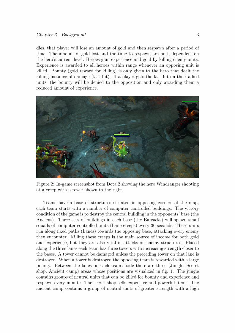
Figure 2: In-game screenshot from Dota 2 showing the hero Windranger shootingat a creep with a tower shown to the right

Teams have a base of structures situated in opposing corners of the map,each team starts with a number of computer controlled buildings. The victorycondition of the game is to destroy the central building in the opponents’ base (theAncient). Three sets of buildings in each base (the Barracks) will spawn smallsquads of computer controlled units (Lane creeps) every 30 seconds. These unitsrun along fixed paths (Lanes) towards the opposing base, attacking every enemythey encounter. Killing these creeps is the main source of income for both goldand experience, but they are also vital in attacks on enemy structures. Placedalong the three lanes each team has three towers with increasing strength closer tothe bases. A tower cannot be damaged unless the preceding tower on that lane isdestroyed. When a tower is destroyed the opposing team is rewarded with a largebounty. Between the lanes on each team’s side there are three (Jungle, Secretshop, Ancient camp) areas whose positions are visualized in fig. 1. The junglecontains groups of neutral units that can be killed for bounty and experience andrespawn every minute. The secret shop sells expensive and powerful items. Theancient camp contains a group of neutral units of greater strength with a high

Chapter 3. Background 4

experience and bounty reward upon death. Situated on the Dire side of the riveris the Roshan pit, where a very powerful neutral unit called Roshan is located.When Roshan is killed a large bounty is given to the team that got the last hiton him. At the same time an item, the Aegis of the Immortal, is dropped thatrevives the carrier upon death and is thereby consumed.

Dota 2 has many possible indicators for which team is ahead, either by showingthe relative strength of the teams like gold and experience or by showing how closethe team is to winning like tower kills. There is however no objective indicatorlike the score in soccer, since the game ends when either team completes theirobjective of destroying the Ancient. To find the relationship between the possibleindicators and the eventual winner of a Dota 2 game this thesis will employ asystematic approach using machine learning.

3.2 Machine LearningMachine learning [8] is a field of computer science that governs systems thatcan learn from data in order to improve performance at a specific task. Withinmachine learning there is a subsection of problems called supervised learning[8], where example inputs are used to create a model which produces a desiredoutput. The inputs are sets of instances where each instance has a vector ofattributes, one of them being the desired output (target attribute). The modelsare constructed attempting to match the relationship from the attributes to thetarget attribute found in the data. If the target attribute is a nominal value, itis called the class and the model a classifier. There is a wide variety of machinelearning algorithms that due to differences in how they operate construct modelsthat function differently internally, even if they produce similar outputs giventhe same input. Using several models constructed from the same or differentalgorithms and then using the mean or mode of those predictions as the finalresult is a technique to get better predictions called ensemble learning. One suchalgorithm is Random Forest (RF) [9] that constructs several trees on randomlysampled subsets of instances and attributes.

Validating that the models built are accurately representing the dataset isan important part of machine learning. K-fold cross validation [10] is a modelvalidation technique, which involves splitting the data into k validation datasets.For every subset a model is built on the data not in that subset. The model isthen used to predict results from the instances in the validation dataset. Thepredicted result from the model is compared to the actual result in the data.Different statistical tests can be performed on those results in order to test themodels accuracy. Accuracy is the percentage of correct guesses, but it is alsoimportant to consider the rates of correct to incorrect guesses for every possibleoutcome of the model. Evaluating these rates gives a deeper insight of how themodel actually performs compared to just looking at the accuracy [11]. The

results will also vary due to random sampling done during the construction of themodel, it is therefore important to test the results using statistical tests.

3.3 Statistical Hypothesis TestingStatistical hypothesis tests are a way of inferring how probable certain hypothesesare from data i.e. how likely is it that a given set of data would arise just fromrandom chance and not because of the proposed relationships in the data. Forexample, given a set of measurements of two different variables a researcher thinksthere’s a relationship between the two. To test this hypothesis the researchercalculates the chance that these measurements could occur assuming the nullhypothesis is true. The null hypothesis is that there is no relationship betweenthe variables and given the value of one variable the other will be random. Thechance of the null hypothesis being true given your data is called the p-value[12]. If the p-value is lower than the significance level, usually 5%, the nullhypothesis is rejected as being unlikely to be true which gives further evidencefor the hypothetical relationship between the variables.

There are many types of statistical tests designed for different types of hy-potheses, analysis of variance (ANOVA) [13] is one such test. ANOVA is per-formed on a grouping of normally distributed data where the null hypothesis isthat the means of all groups are equal. It is used to determine whether there aredifferences between the groups and if they can be distinguished from each otherin the data. For example, given a distribution of cars over their max velocities, agrouping based on chassis color would not create groups with different mean maxvelocities because there is no relation between the two attributes. This wouldresult in a high p-value in an ANOVA test. Grouping the same distributionbased on the cars models would result in differences between the groups and alow p-value from an ANOVA test. ANOVA is designed to work on data that isnormally distributed without large differences in the variance of the groups, bothof these properties should be tested before using ANOVA to prevent errors inthe conclusion. Since ANOVA only tests whether there is any difference betweenthe groups, but not which group or groups are diverging, a common follow up isTukey’s Test [14].

Tukey’s Test performs a comparison of means for all possible pairwise combi-nations of the groups. For each combination it tests if the difference between thetwo means is less than the standard error. The standard error [15] is the expecteddifference between the mean of a sampled distribution and the actual mean ofthe distribution it is sampled from. The Tukey’s Test therefore gives the prob-ability of two groups being similar samples of a bigger distribution. To give anexample using the same scenario as before with cars, when grouping the cars bymodel the comparison between two brands of sports cars will give a high p-valuein the Tukey’s Test since they have similar distributions of max velocities, but

5

comparing one brand of sports cars with a brand of vans will give a low p-value.

4. ObjectivesIn this thesis an attempt was made to determine the effectiveness of machinelearning techniques with a focus on Random Forest, when applied to classifyingthe result of Dota 2 games. This was done using partial game-state data that isindicative of success without relying on the specific hero lineups of the teams. Totry and prevent the results from becoming irrelevant with future patches, herolineups were omitted. Patches tend to change hero lineups more than they doitem purchases or the importance of objectives on the map. Instead the focuswas set on indicators of which team is currently winning for example Hero Kills,Roshan Kills, Items, and more as detailed in Appendix A.

4.1 Research QuestionsRQ1 What is the highest average accuracy achievable using different parameters

of the Random Forest algorithm?

RQ2 How does the average accuracy of the model vary at different gametimes?

RQ3 What is the relationship between the parameters of the algorithm and thetraining and validation time?

5. Method5.1 Data AcquisitionDuring the initial research no way was found to adequately acquire the quantity ofreplays needed for the experiments. Dota 2 has an average of 450 000 concurrentplayers1 and every match played has a replay temporarily saved on Valve’s servers.To get these replays, a way of retrieving a list of recently played games was needed.This was done through Valve’s WebAPI2 described in Appendix C.

In order to download a replay, a so-called replay salt is needed which is notprovided through the WebAPI, but can be retrieved through the Dota 2 client. Aprogram based on SteamRE3 was made in order to retrieve the necessary infor-mation. Combining both the WebAPI data and replay salt made the downloadspossible.

1http://steamgraph.net/index.php?action=graph&appid=570 Accessed: 10-4-20132http://dev.dota2.com/showthread.php?t=58317 Accessed: 6-1-20153https://github.com/SteamRE/SteamKit Accessed: 6-1-2015

6

Chapter 5. Method 7

Replays of 15146 games were gathered, consisting only of games with the AP(all pick) game mode in the very high skill bracket, played during the periodfrom 2013-02-28 to 2013-04-15 at all times of the day. It was decided to limit thesampling and only include the very high skill bracket to ensure the best qualityof play available in public games. It is important to note that no major balancepatch1 was deployed during the replay acquisition period, as such an event mighthave had an impact on the dataset.

5.2 Data ParsingDota 2 game replays are saved in the DEM Format2, compressed using bzip2and named after their MatchID, for example "137725678.dem.bz2". Valve doesnot provide a parser that extracts all the information contained in the replay,which lead the community to produce a number of parsers. Among them is anopen source replay parser in Python called Tarrasque3, that was used to print thenetwork packets stored in the replay file into plain text. This parser was modifiedto extract the current game-state at each minute. Contributions to Tarrasquewere made in order to extract the specific data needed4.

The output from Tarrasque was converted to the "Raw" format as seen inAppendix A. This was done as parsing replays using Tarrasque was by far themost time consuming part of the entire data processing procedure (there are nownewer and faster parsers, one example is Clarity5, a Java based parser). A simplePython parser was made to convert the raw game-state data into the format, asseen in Team Advantage, Appendix B.

5.3 Preliminary ExperimentThe initial hypothesis was that RF would be a good candidate for the datasetbecause it has shown to be among the best algorithms in other studies [16] [17][18]. This hypothesis was tested by comparing RF with algorithms from differentfamilies. All the classifiers were tested with default settings in R6 and multiplek-fold cross validation tests were performed with varying seeds. The classifierswere compared based on their accuracy, True Radiant Rate (TRR), and True DireRate (TDR). TRR is the rate of correctly classified instances from games whereRadiant won and TDR is equivalent for the instances were Dire won. TRR and

1http://dota2.gamepedia.com/Patches Accessed: 6-1-20152https://developer.valvesoftware.com/wiki/DEM_Format Accessed: 6-1-20153https://github.com/skadistats/Tarrasque Accessed: 6-1-20154https://github.com/skadistats/Tarrasque/commits?author=Truth- Accessed: 6-1-20155https://github.com/skadistats/clarity Accessed: 6-1-20156http://www.r-project.org/ Accessed: 6-1-2015

Chapter 5. Method 8

TDR is the sensitivity and specificity [32] of the classification, but are renamedbecause there is no positive or negative result of a Dota 2 game.

5.3.1 Algorithms

RF operates by constructing multiple decision trees. For each tree a new datasetof equal size to the training set is constructed by random sampling with replace-ment (bootstrapping [19]) from the original training set. Sampling with replace-ment means that an instance already added to the subset can be added again, theset will therefore contain some duplicates. During the construction of every tree,each node in the tree only considers a random selection of attributes, choosingthe attribute that best splits the set of classes. When making predictions themajority vote from all trees in the model is used. This method of sampling andvoting is called bootstrap aggregating or bagging [20].

LibSVM [21] is a library that implements an algorithm from the SupportVector Machine (SVM) [22] family, and was chosen as it had promising resultsin previous research [23]. SVM works by treating instances of the training set asspatial vectors. It then finds a single or set of hyperplanes that divides up thespace between instances of different classes and has the greatest distance to theirclosest instances. Kernel functions can be used to transform all the instancesinto a higher dimensional space to find planes between classes, which originallycould not be separated in their original space. Classifying new instances is doneby putting the instance in that space and assigning it to the same class as theinstances on the same side of the hyperplane or hyperplanes. The resulting modelis quite complex and hard to decipher due to the nature of the algorithm makingSVMs often regarded as black-box solutions.

The Naive Bayes (NB) [24] classifier is often used in problems with text cat-egorization and has proven to be good in earlier empirical studies [25]. NaiveBayes is trained by calculating for each class the mean and variance of the at-tributes of every instance that belong to that class. An instances predicted classis then the class that has the most probable match given the means and variancescalculated in training. The Naive Bayes algorithm thereby creates a simple modelthat considers all attributes independently when assigning a class, ignoring anyco-variance.

The ensemble family encompasses classifiers built on different techniques, bag-ging and boosting [26]. LogitBoost was chosen has proven to be good in severalstudies [28], and is a variant of AdaBoost [29] which is a Meta Algorithm thatuses multiple simple machine learning algorithms, so called weak learners. Logit-Boost [27] is also built around boosting in contrast to RFs bagging. Boosting is amethod where all instances of data will have an associated weight. These weightsare used by the weak learners when constructing the model (a higher weight ismore important to guess correctly). The weights are changed after every iter-ation, correctly guessed instances gets decreased and incorrectly gets increased.

Chapter 5. Method 9

After a defined amount of iterations the resulting models are combined to makea final complex model.

The last chosen algorithm for this experiment was NNge [30] which comesfrom the k-Nearest Neighbour (k-NN) algorithm family. NNge is k-NN withgeneralization and has been used successfully in previous studies [31]. NNgetreats instances of the training set as spatial vectors, and generalizes groups ofinstances with the same class that are close to each other into non-overlappinghyperrectangles. Predicting the class of a new instance is done by finding theclass of the nearest instance or hyperrectangle.

5.3.2 Results and Conclusion

During the early stages of evaluation it was discovered that several of the classifi-cation algorithms were not suited for the dataset. NNge and LibSVM had trainingtimes of over 12 hours on just a subset the dataset and were thus dismissed fromfuture tests. The three remaining classifiers were all tested with two data sourcesdescribed in Appendix A and Appendix B, with and without correlation-basedattribute selection.

Algorithm Parameters Accuracy TRR TDR

NaiveBayesNone Team Advg. 85.4% 0.883 0.814

Raw Data 77.3% 0.963 0.652

Attri. Selct. Team Advg. 79.2% 0.837 0.733Raw Data 75.8% 0.713 0.950

Random ForestNone Team Advg. 88.7% 0.886 0.888

Raw Data 89.4% 0.888 0.903

Attri. Selct. Team Advg. 82.4% 0.825 0.823Raw Data 78.1% 0.738 0.927

LogitBoostNone Team Advg. 83.1% 0.838 0.820

Raw Data 79.2% 0.837 0.733

Attri. Selct. Team Advg. 84.1% 0.808 0.915Raw Data 78.1% 0.738 0.927

TRR = True Radiant Rate, TDR = True Dire Rate

Table 1: Preliminary Experiment Results

The results in table 1 shows that RF, no selection, with raw data formatoutperformed the others in average accuracy. Because of this it was decidedthat future experiments would solely revolve around RF and determining howparameter tuning would change its accuracy.

5.4 Training and Validation SubsetsFor each execution of the main experiments, training and validation subsets wereconstructed by grouping all instances into games by MatchId and randomly sam-pling 20% of all games into the validation set, with the remaining forming the

Chapter 5. Method 10

training set. This was done in order to ensure that there was no interdependencebetween instances of the training and validation set. An experiment was per-formed to make sure that the mean average game-time of the validation sets didnot vary too much from the average game-time of the total set of games, as thiswould be an indication of an error in the sampling method.

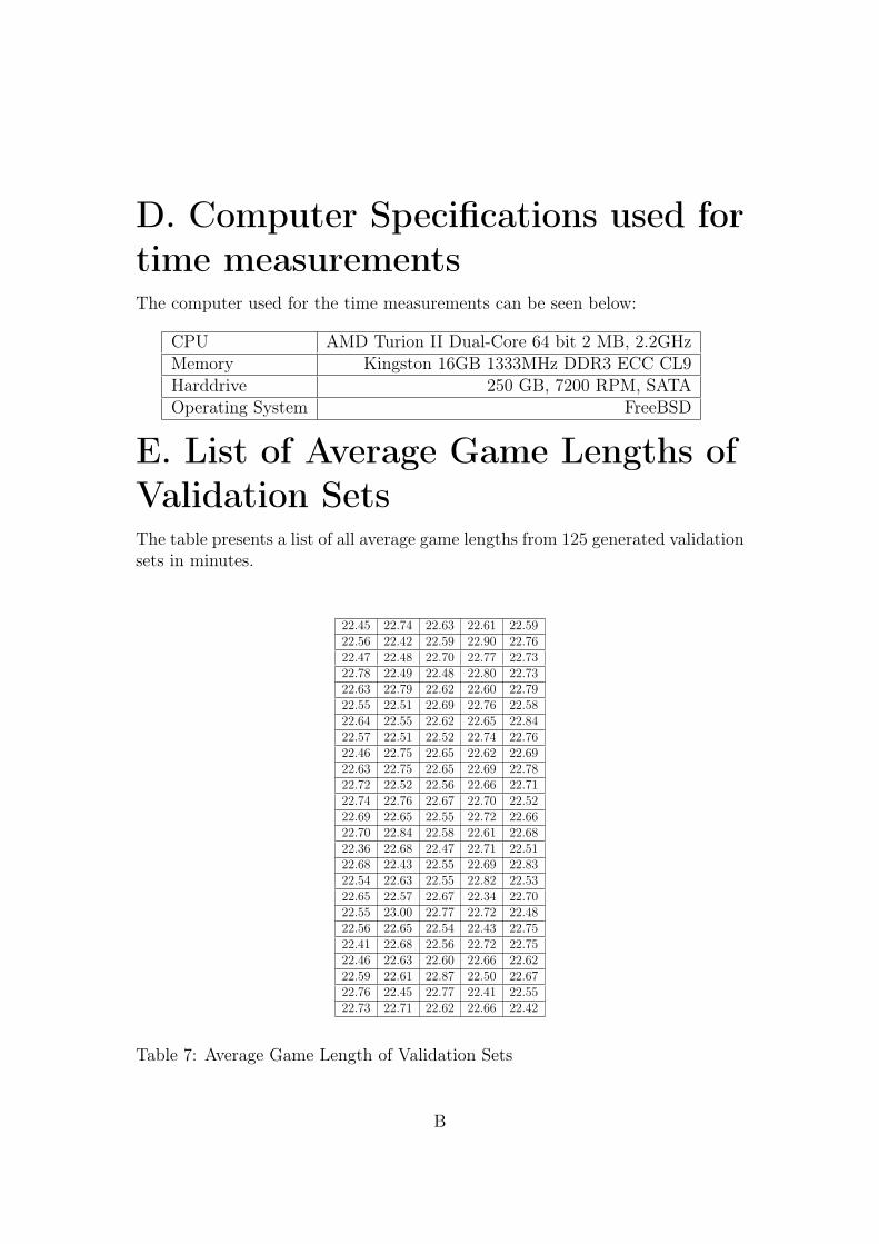
The sampling used to create the validation sets was evaluated by comparingthe distribution of average game-lengths from generated validation sets to theaverage game-length of all games. Specifically if the average game-length of allgames lay within the confidence interval of the distributions mean average game-length at a confidence level of 0.975.

Label ValueStandard Deviation 0.125Confidence Coefficient 0.975Confidence Interval Min 22.617Confidence Interval Max 22.649Average GameLength of all Games 22.632

Table 2: ValidationSet GameTime Data

From 125 generated validationsets the average game-lengths wererecorded, these are listed in Ap-pendix E. The standard deviation ofthose averages and the confidence in-terval of the mean average game-lengthfor a confidence coefficient of 0.975 islisted in table 2. The average game-length of all games lies within this in-terval. The specifications of the computer used to run the experiments can beseen in Appendix D.

The distribution of average game-lengths of the validation sets from Ap-pendix E was plotted using a density plot (fig. 3). All the average times fellwithin twenty seconds of the average game-length of the entire set of games. Be-cause the true mean average game-length of the validation sets lies in the intervalgiven in table 2 with a 97.5% confidence level, there is no indication of an errorduring the sampling process.

Chapter 5. Method 11

Avg

. Gam

e Le

ngth

of A

ll G

ames

Avg

. Gam

e Le

ngth

of A

ll G

ames

Avg

. Gam

e Le

ngth

of A

ll G

ames

Avg

. Gam

e Le

ngth

of A

ll G

ames

Avg

. Gam

e Le

ngth

of A

ll G

ames

Avg

. Gam

e Le

ngth

of A

ll G

ames

Avg

. Gam

e Le

ngth

of A

ll G

ames

Avg

. Gam

e Le

ngth

of A

ll G

ames

Avg

. Gam

e Le

ngth

of A

ll G

ames

Avg

. Gam

e Le

ngth

of A

ll G

ames

Avg

. Gam

e Le

ngth

of A

ll G

ames

Avg

. Gam

e Le

ngth

of A

ll G

ames

Avg

. Gam

e Le

ngth

of A

ll G

ames

Avg

. Gam

e Le

ngth

of A

ll G

ames

Avg

. Gam

e Le

ngth

of A

ll G

ames

Avg

. Gam

e Le

ngth

of A

ll G

ames

Avg

. Gam

e Le

ngth

of A

ll G

ames

Avg

. Gam

e Le

ngth

of A

ll G

ames

Avg

. Gam

e Le

ngth

of A

ll G

ames

Avg

. Gam

e Le

ngth

of A

ll G

ames

Avg

. Gam

e Le

ngth

of A

ll G

ames

Avg

. Gam

e Le

ngth

of A

ll G

ames

Avg

. Gam

e Le

ngth

of A

ll G

ames

Avg

. Gam

e Le

ngth

of A

ll G

ames

Avg

. Gam

e Le

ngth

of A

ll G

ames

Avg

. Gam

e Le

ngth

of A

ll G

ames

Avg

. Gam

e Le

ngth

of A

ll G

ames

Avg

. Gam

e Le

ngth

of A

ll G

ames

Avg

. Gam

e Le

ngth

of A

ll G

ames

Avg

. Gam

e Le

ngth

of A

ll G

ames

Avg

. Gam

e Le

ngth

of A

ll G

ames

Avg

. Gam

e Le

ngth

of A

ll G

ames

Avg

. Gam

e Le

ngth

of A

ll G

ames

Avg

. Gam

e Le

ngth

of A

ll G

ames

Avg

. Gam

e Le

ngth

of A

ll G

ames

Avg

. Gam

e Le

ngth

of A

ll G

ames

Avg

. Gam

e Le

ngth

of A

ll G

ames

Avg

. Gam

e Le

ngth

of A

ll G

ames

Avg

. Gam

e Le

ngth

of A

ll G

ames

Avg

. Gam

e Le

ngth

of A

ll G

ames

Avg

. Gam

e Le

ngth

of A

ll G

ames

Avg

. Gam

e Le

ngth

of A

ll G

ames

Avg

. Gam

e Le

ngth

of A

ll G

ames

Avg

. Gam

e Le

ngth

of A

ll G

ames

Avg

. Gam

e Le

ngth

of A

ll G

ames

Avg

. Gam

e Le

ngth

of A

ll G

ames

Avg

. Gam

e Le

ngth

of A

ll G

ames

Avg

. Gam

e Le

ngth

of A

ll G

ames

Avg

. Gam

e Le

ngth

of A

ll G

ames

Avg

. Gam

e Le

ngth

of A

ll G

ames

Avg

. Gam

e Le

ngth

of A

ll G

ames

Avg

. Gam

e Le

ngth

of A

ll G

ames

Avg

. Gam

e Le

ngth

of A

ll G

ames

Avg

. Gam

e Le

ngth

of A

ll G

ames

Avg

. Gam

e Le

ngth

of A

ll G

ames

Avg

. Gam

e Le

ngth

of A

ll G

ames

Avg

. Gam

e Le

ngth

of A

ll G

ames

Avg

. Gam

e Le

ngth

of A

ll G

ames

Avg

. Gam

e Le

ngth

of A

ll G

ames

Avg

. Gam

e Le

ngth

of A

ll G

ames

Avg

. Gam

e Le

ngth

of A

ll G

ames

Avg

. Gam

e Le

ngth

of A

ll G

ames

Avg

. Gam

e Le

ngth

of A

ll G

ames

Avg

. Gam

e Le

ngth

of A

ll G

ames

Avg

. Gam

e Le

ngth

of A

ll G

ames

Avg

. Gam

e Le

ngth

of A

ll G

ames

Avg

. Gam

e Le

ngth

of A

ll G

ames

Avg

. Gam

e Le

ngth

of A

ll G

ames

Avg

. Gam

e Le

ngth

of A

ll G

ames

Avg

. Gam

e Le

ngth

of A

ll G

ames

Avg

. Gam

e Le

ngth

of A

ll G

ames

Avg

. Gam

e Le

ngth

of A

ll G

ames

Avg

. Gam

e Le

ngth

of A

ll G

ames

Avg

. Gam

e Le

ngth

of A

ll G

ames

Avg

. Gam

e Le

ngth

of A

ll G

ames

Avg

. Gam

e Le

ngth

of A

ll G

ames

Avg

. Gam

e Le

ngth

of A

ll G

ames

Avg

. Gam

e Le

ngth

of A

ll G

ames

Avg

. Gam

e Le

ngth

of A

ll G

ames

Avg

. Gam

e Le

ngth

of A

ll G

ames

Avg

. Gam

e Le

ngth

of A

ll G

ames

Avg

. Gam

e Le

ngth

of A

ll G

ames

Avg

. Gam

e Le

ngth

of A

ll G

ames

Avg

. Gam

e Le

ngth

of A

ll G

ames

Avg

. Gam

e Le

ngth

of A

ll G

ames

Avg

. Gam

e Le

ngth

of A

ll G

ames

Avg

. Gam

e Le

ngth

of A

ll G

ames

Avg

. Gam

e Le

ngth

of A

ll G

ames

Avg

. Gam

e Le

ngth

of A

ll G

ames

Avg

. Gam

e Le

ngth

of A

ll G

ames

Avg

. Gam

e Le

ngth

of A

ll G

ames

Avg

. Gam

e Le

ngth

of A

ll G

ames

Avg

. Gam

e Le

ngth

of A

ll G

ames

Avg

. Gam

e Le

ngth

of A

ll G

ames

Avg

. Gam

e Le

ngth

of A

ll G

ames

Avg

. Gam

e Le

ngth

of A

ll G

ames

Avg

. Gam

e Le

ngth

of A

ll G

ames

Avg

. Gam

e Le

ngth

of A

ll G

ames

Avg

. Gam

e Le

ngth

of A

ll G

ames

Avg

. Gam

e Le

ngth

of A

ll G

ames

Avg

. Gam

e Le

ngth

of A

ll G

ames

Avg

. Gam

e Le

ngth

of A

ll G

ames

Avg

. Gam

e Le

ngth

of A

ll G

ames

Avg

. Gam

e Le

ngth

of A

ll G

ames

Avg

. Gam

e Le

ngth

of A

ll G

ames

Avg

. Gam

e Le

ngth

of A

ll G

ames

Avg

. Gam

e Le

ngth

of A

ll G

ames

Avg

. Gam

e Le

ngth

of A

ll G

ames

Avg

. Gam

e Le

ngth

of A

ll G

ames

Avg

. Gam

e Le

ngth

of A

ll G

ames

Avg

. Gam

e Le

ngth

of A

ll G

ames

Avg

. Gam

e Le

ngth

of A

ll G

ames

Avg

. Gam

e Le

ngth

of A

ll G

ames

Avg

. Gam

e Le

ngth

of A

ll G

ames

Avg

. Gam

e Le

ngth

of A

ll G

ames

Avg

. Gam

e Le

ngth

of A

ll G

ames

Avg

. Gam

e Le

ngth

of A

ll G

ames

Avg

. Gam

e Le

ngth

of A

ll G

ames

Avg

. Gam

e Le

ngth

of A

ll G

ames

Avg

. Gam

e Le

ngth

of A

ll G

ames

Avg

. Gam

e Le

ngth

of A

ll G

ames

Avg

. Gam

e Le

ngth

of A

ll G

ames

Avg

. Gam

e Le

ngth

of A

ll G

ames

Avg

. Gam

e Le

ngth

of A

ll G

ames

Avg

. Gam

e Le

ngth

of A

ll G

ames

Avg

. Gam

e Le

ngth

of A

ll G

ames

Avg

. Gam

e Le

ngth

of A

ll G

ames

Avg

. Gam

e Le

ngth

of A

ll G

ames

Avg

. Gam

e Le

ngth

of A

ll G

ames

Avg

. Gam

e Le

ngth

of A

ll G

ames

Avg

. Gam

e Le

ngth

of A

ll G

ames

Avg

. Gam

e Le

ngth

of A

ll G

ames

Avg

. Gam

e Le

ngth

of A

ll G

ames

Avg

. Gam

e Le

ngth

of A

ll G

ames

Avg

. Gam

e Le

ngth

of A

ll G

ames

Avg

. Gam

e Le

ngth

of A

ll G

ames

Avg

. Gam

e Le

ngth

of A

ll G

ames

Avg

. Gam

e Le

ngth

of A

ll G

ames

Avg

. Gam

e Le

ngth

of A

ll G

ames

Avg

. Gam

e Le

ngth

of A

ll G

ames

Avg

. Gam

e Le

ngth

of A

ll G

ames

Avg

. Gam

e Le

ngth

of A

ll G

ames

Avg

. Gam

e Le

ngth

of A

ll G

ames

Avg

. Gam

e Le

ngth

of A

ll G

ames

Avg

. Gam

e Le

ngth

of A

ll G

ames

Avg

. Gam

e Le

ngth

of A

ll G

ames

Avg

. Gam

e Le

ngth

of A

ll G

ames

Avg

. Gam

e Le

ngth

of A

ll G

ames

Avg

. Gam

e Le

ngth

of A

ll G

ames

Avg

. Gam

e Le

ngth

of A

ll G

ames

Avg

. Gam

e Le

ngth

of A

ll G

ames

Avg

. Gam

e Le

ngth

of A

ll G

ames

Avg

. Gam

e Le

ngth

of A

ll G

ames

Avg

. Gam

e Le

ngth

of A

ll G

ames

Avg

. Gam

e Le

ngth

of A

ll G

ames

Avg

. Gam

e Le

ngth

of A

ll G

ames

Avg

. Gam

e Le

ngth

of A

ll G

ames

Avg

. Gam

e Le

ngth

of A

ll G

ames

Avg

. Gam

e Le

ngth

of A

ll G

ames

Avg

. Gam

e Le

ngth

of A

ll G

ames

Avg

. Gam

e Le

ngth

of A

ll G

ames

Avg

. Gam

e Le

ngth

of A

ll G

ames

Avg

. Gam

e Le

ngth

of A

ll G

ames

Avg

. Gam

e Le

ngth

of A

ll G

ames

Avg

. Gam

e Le

ngth

of A

ll G

ames

Avg

. Gam

e Le

ngth

of A

ll G

ames

Avg

. Gam

e Le

ngth

of A

ll G

ames

Avg

. Gam

e Le

ngth

of A

ll G

ames

Avg

. Gam

e Le

ngth

of A

ll G

ames

Avg

. Gam

e Le

ngth

of A

ll G

ames

Avg

. Gam

e Le

ngth

of A

ll G

ames

Avg

. Gam

e Le

ngth

of A

ll G

ames

Avg

. Gam

e Le

ngth

of A

ll G

ames

Avg

. Gam

e Le

ngth

of A

ll G

ames

Avg

. Gam

e Le

ngth

of A

ll G

ames

Avg

. Gam

e Le

ngth

of A

ll G

ames

Avg

. Gam

e Le

ngth

of A

ll G

ames

Avg

. Gam

e Le

ngth

of A

ll G

ames

Avg

. Gam

e Le

ngth

of A

ll G

ames

Avg

. Gam

e Le

ngth

of A

ll G

ames

Avg

. Gam

e Le

ngth

of A

ll G

ames

Avg

. Gam

e Le

ngth

of A

ll G

ames

Avg

. Gam

e Le

ngth

of A

ll G

ames

Avg

. Gam

e Le

ngth

of A

ll G

ames

Avg

. Gam

e Le

ngth

of A

ll G

ames

Avg

. Gam

e Le

ngth

of A

ll G

ames

Avg

. Gam

e Le

ngth

of A

ll G

ames

Avg

. Gam

e Le

ngth

of A

ll G

ames

Avg

. Gam

e Le

ngth

of A

ll G

ames

Avg

. Gam

e Le

ngth

of A

ll G

ames

Avg

. Gam

e Le

ngth

of A

ll G

ames

Avg

. Gam

e Le

ngth

of A

ll G

ames

Avg

. Gam

e Le

ngth

of A

ll G

ames

Avg

. Gam

e Le

ngth

of A

ll G

ames

Avg

. Gam

e Le

ngth

of A

ll G

ames

Avg

. Gam

e Le

ngth

of A

ll G

ames

Avg

. Gam

e Le

ngth

of A

ll G

ames

Avg

. Gam

e Le

ngth

of A

ll G

ames

Avg

. Gam

e Le

ngth

of A

ll G

ames

Avg

. Gam

e Le

ngth

of A

ll G

ames

Avg

. Gam

e Le

ngth

of A

ll G

ames

Avg

. Gam

e Le

ngth

of A

ll G

ames

Avg

. Gam

e Le

ngth

of A

ll G

ames

Avg

. Gam

e Le

ngth

of A

ll G

ames

Avg

. Gam

e Le

ngth

of A

ll G

ames

Avg

. Gam

e Le

ngth

of A

ll G

ames

Avg

. Gam

e Le

ngth

of A

ll G

ames

Avg

. Gam

e Le

ngth

of A

ll G

ames

Avg

. Gam

e Le

ngth

of A

ll G

ames

Avg

. Gam

e Le

ngth

of A

ll G

ames

Avg

. Gam

e Le

ngth

of A

ll G

ames

Avg

. Gam

e Le

ngth

of A

ll G

ames

Avg

. Gam

e Le

ngth

of A

ll G

ames

Avg

. Gam

e Le

ngth

of A

ll G

ames

Avg

. Gam

e Le

ngth

of A

ll G

ames

Avg

. Gam

e Le

ngth

of A

ll G

ames

Avg

. Gam

e Le

ngth

of A

ll G

ames

Avg

. Gam

e Le

ngth

of A

ll G

ames

Avg

. Gam

e Le

ngth

of A

ll G

ames

Avg

. Gam

e Le

ngth

of A

ll G

ames

Avg

. Gam

e Le

ngth

of A

ll G

ames

Avg

. Gam

e Le

ngth

of A

ll G

ames

Avg

. Gam

e Le

ngth

of A

ll G

ames

Avg

. Gam

e Le

ngth

of A

ll G

ames

Avg

. Gam

e Le

ngth

of A

ll G

ames

Avg

. Gam

e Le

ngth

of A

ll G

ames

Avg

. Gam

e Le

ngth

of A

ll G

ames

Avg

. Gam

e Le

ngth

of A

ll G

ames

Avg

. Gam

e Le

ngth

of A

ll G

ames

Avg

. Gam

e Le

ngth

of A

ll G

ames

Avg

. Gam

e Le

ngth

of A

ll G

ames

Avg

. Gam

e Le

ngth

of A

ll G

ames

Avg

. Gam

e Le

ngth

of A

ll G

ames

Avg

. Gam

e Le

ngth

of A

ll G

ames

Avg

. Gam

e Le

ngth

of A

ll G

ames

Avg

. Gam

e Le

ngth

of A

ll G

ames

Avg

. Gam

e Le

ngth

of A

ll G

ames

Avg

. Gam

e Le

ngth

of A

ll G

ames

Avg

. Gam

e Le

ngth

of A

ll G

ames

Avg

. Gam

e Le

ngth

of A

ll G

ames

Avg

. Gam

e Le

ngth

of A

ll G

ames

Avg

. Gam

e Le

ngth

of A

ll G

ames

Avg

. Gam

e Le

ngth

of A

ll G

ames

0.00

0.25

0.50

0.75

1.00

22.4 22.6 22.8Game Length

Den

sity

Figure 3: Distribution of Average Game Lengths from Validation Sets

5.5 ExperimentsWith the focus on RF, Parameter Exploration was performed in order to find theanswer to RQ1 and RQ3. The answer to RQ2 was studied in RF Comparisons.

5.5.1 Parameter Exploration

To try and find the optimal parameters for RF, all possible combinations of{1,3,5,7,9} attributes and {10, 60, 110, 160, 210} trees, were trained and vali-dated five times each with new validation and training sets every time. For eachparameter combination a measurement of the average accuracy, the time it tookto train the model, and the time it took to validate the model was recorded. Theparameters were chosen to cover a wide, evenly spaced range.

5.5.2 Random Forest Comparisons

From the results of the Parameter Exploration experiment it was decided tomake a more in depth comparison between a parameterized RF with 210 trees 9attributes, RF with default settings, and a majority class classifier. The defaultsetting for RF in WEKA given dataset the used in this thesis was 100 trees and 8

attributes. The average accuracy of all three models was measured and recordedon a per minute of game-time basis.

5.6 EvaluationTo determine which parameters had the largest impact on accuracy, an ANOVATest was performed on the resulting distribution of prediction accuracies of alldifferent parameter combinations with the results divided into two groupings bynumber of trees or number of attributes. Since ANOVA has requirements on thedata a Shapiro-Wilk [33] normality test and Levene’s Test [34] for homogeneity ofvariance was performed. Shapiro-Wilk test result was a p-value of 0.9072 and thusthe null hypothesis of normality was accepted. Levene’s Test resulted in a p-valueof 0.9503 and thus the null hypothesis of homogeneity of variance was accepted.Any variance between the means detected would then be further explored with aTukey’s Test to find out which parameters diverged the most from the means ofthe other groups.

6. ResultsThe results from the parameter exploration experiment are listed in table 3. TheTrue Radiant Rate (TRR) doesn’t improve with different parameters, only TrueDire Rate (TDR) performs better. The Validation Time (VT) increases with thenumber of trees but decreases with the number of attributes. Training Time (TT)scales with both parameters.

12

Trees Attributes Accuracy TRR TDR TT VT10 1 86.49% 0.926 0.777 1.96 0.110 3 86.91% 0.924 0.790 2.4 0.0810 5 87.23% 0.923 0.800 2.85 0.0810 7 87.55% 0.926 0.803 3.39 0.0810 9 87.50% 0.924 0.804 3.83 0.0860 1 88.16% 0.925 0.819 11.41 0.3660 3 88.26% 0.925 0.824 13.78 0.2860 5 88.44% 0.924 0.828 16.9 0.2460 7 88.58% 0.923 0.833 20.08 0.2260 9 88.57% 0.921 0.835 22.98 0.21110 1 88.41% 0.926 0.825 20.61 0.86110 3 88.48% 0.925 0.830 25.27 0.6110 5 88.63% 0.924 0.833 30.92 0.48110 7 88.61% 0.922 0.836 36.54 0.43110 9 88.74% 0.922 0.839 42.41 0.4160 1 88.48% 0.926 0.827 30.47 1.48160 3 88.58% 0.922 0.833 37.08 1.02160 5 88.66% 0.922 0.836 44.55 0.82160 7 88.63% 0.922 0.836 53.45 0.71160 9 88.78% 0.925 0.836 61.25 0.64210 1 88.35% 0.924 0.824 38.5 2.07210 3 88.51% 0.923 0.831 49.06 1.47210 5 88.66% 0.923 0.835 59.4 1.19210 7 88.78% 0.922 0.839 70.16 1.02210 9 88.83% 0.922 0.840 80.03 0.91TRR = True Radiant Rate, TDR = True Dire Rate,TT = Training Time, V T = Validation Time

Table 3: Average of Raw Data with Different Parameters, the Training and Vali-dation Time displays average in number of minutes it took to execute

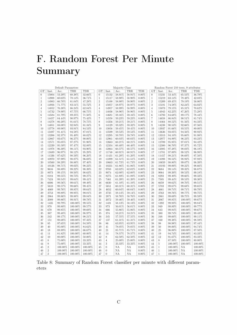
The table 4 contains a summary of the results from the RF comparisonsbetween default parameters, 210 trees 9 attributes, and a majority class classifier.A more detailed summary for each minute of game-time is listed in Appendix F.

Classifier Instances Accuracy TRR TDRMajority Class 357984 59.97% 0.600 0.000Default 355539 87.41% 0.926 0.802210 Trees - 9 Attributes 359486 88.83% 0.922 0.840TRR = True Radiant Rate, TDR = True Dire Rate

Table 4: Random Forest Summary

13

Chapter 7. Analysis 14

7. AnalysisAs seen in fig. 4 the number of trees has the largest positive impact on accuracy.This increase however diminishes with a high number of trees, while an increasein attributes is still contributing to an increase in accuracy. This is corroboratedby the ANOVA Test in table 5 and the Tukey’s Test in table 6. The p-valueis lower for the Trees group than the Attributes group in the ANOVA test butlooking at the Tukey’s Test 110-210 trees has a higher value than 5-9 attributes,the greatest difference for trees is when increasing from 10 to 60.

O

O

OO

O

86.5%

87.0%

87.5%

88.0%

88.5%

0 50 100 150 200Number Trees

Per

cent

Number Attributes

O 1

3

5

7

9

Figure 4: Random Forest Accuracy with different number Trees/Attributes

Variable n M SD t pTrees 4 0.004018 0.0010044 149.35 < 2e-16Attributes 4 0.000435 0.0001086 16.16 1.59e-10M = mean, SD = standard deviation

Table 5: ANOVA Test on Parameter Experiment grouped by Trees and Attributes

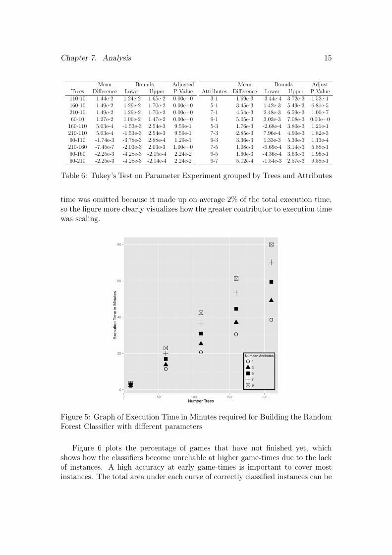
The time required for building the classifiers scales linearly with either factorand exponentially if you increase both, as can be seen in fig. 5. The validation

Chapter 7. Analysis 15

Mean Bounds AdjustedTrees Difference Lower Upper P-Value110-10 1.44e-2 1.24e-2 1.65e-2 0.00e+0160-10 1.49e-2 1.29e-2 1.70e-2 0.00e+0210-10 1.49e-2 1.29e-2 1.70e-2 0.00e+060-10 1.27e-2 1.06e-2 1.47e-2 0.00e+0160-110 5.03e-4 -1.53e-3 2.54e-3 9.59e-1210-110 5.03e-4 -1.53e-3 2.54e-3 9.59e-160-110 -1.74e-3 -3.78e-3 2.88e-4 1.29e-1210-160 -7.45e-7 -2.03e-3 2.03e-3 1.00e+060-160 -2.25e-3 -4.28e-3 -2.15e-4 2.24e-260-210 -2.25e-3 -4.28e-3 -2.14e-4 2.24e-2

Mean Bounds AdjustAttributes Difference Lower Upper P-Value

3-1 1.69e-3 -3.44e-4 3.72e-3 1.52e-15-1 3.45e-3 1.42e-3 5.49e-3 6.81e-57-1 4.54e-3 2.48e-3 6.59e-3 1.00e-79-1 5.05e-3 3.02e-3 7.08e-3 0.00e+05-3 1.76e-3 -2.68e-4 3.80e-3 1.21e-17-3 2.85e-3 7.96e-4 4.90e-3 1.82e-39-3 3.36e-3 1.33e-3 5.39e-3 1.13e-47-5 1.08e-3 -9.69e-4 3.14e-3 5.88e-19-5 1.60e-3 -4.36e-4 3.63e-3 1.96e-19-7 5.12e-4 -1.54e-3 2.57e-3 9.58e-1

Table 6: Tukey’s Test on Parameter Experiment grouped by Trees and Attributes

time was omitted because it made up on average 2% of the total execution time,so the figure more clearly visualizes how the greater contributor to execution timewas scaling.

O

O

O

O

O

0

20

40

60

80

0 50 100 150 200Number Trees

Exe

cutio

n T

ime

in M

inut

es

Number Attributes

O 1

3

5

7

9

Figure 5: Graph of Execution Time in Minutes required for Building the RandomForest Classifier with different parameters

Figure 6 plots the percentage of games that have not finished yet, whichshows how the classifiers become unreliable at higher game-times due to the lackof instances. A high accuracy at early game-times is important to cover mostinstances. The total area under each curve of correctly classified instances can be

Chapter 7. Analysis 16

deceiving because the number of instances at every minute drops quickly after 20.By plotting the product of accuracy and "unfinished games", the area under thatplot becomes equal to the number of correctly classified instances (as shown infig. 7), which better shows how many instances are correctly classified per minute.

0M

25M

50M

75M

100M

0 5 10 15 20 25 30 35 40 45GameTime

Per

cent

ofG

ames

Correctly, Classified, w/, RF, 210, trees, 9, attributes

Correctly, Classified, w/, RF, Default Parameters

Majority Class Classifier

Unfinished,Games

Figure 6: Comparison of Random Forest with two different Parameters, MajorityClass and a line representing the number of unfinished games

0A

25A

50A

75A

100A

0 5 10 15 20 25 30 35 40 45GameTime

Per

cent

ofG

ames

Correctly Classified *FUnfinishedFGames

Random Forest with Raw Data, 210 Trees and 9 Attributes

UnfinishedFGames

Figure 7: Random Forest accuracy scaled with the amount of unfinished yet

As seen in table 3 the TRR doesn’t vary much between different parametersin the RF classifiers and most increase in accuracy is due to the TDR. In fig. 8

this gap between the TDRs of the parameterized and default version of RF can beclearly seen, and it also seems to suggest that the unreliability at high game-timesis also due to TDR. There is not much that differentiates Dire from Radiant, sothis result is unexpected and no explanation for it was found.

0%

25%

50%

75%

100%

0 5 10 15 20 25 30 35 40 45GameTime

Per

cent

210 trees, 9 attributes TDR

210 trees, 9 attributes TRR

Default TDR

Default TRR

Figure 8: True Radiant Rate and True Dire Rate graphed from Random Forestwith default and 210 trees with 9 attributes

8. ConclusionsIn this thesis many differently parameterized versions of the RF classificationalgorithm were used to predict Dota 2 results using partial gamestate data withouthero lineups. The results achieved were better than expected but there is a lotmore that could have been done.

As seen in table 3 the best model had an average accuracy of 88.83%, whichis higher than expected because it was thought that there would be less of adifference between the teams during the first 5 minutes to be used as a basis forclassification. However, as seen in fig. 6, the model is already correctly predict-ing 82.23% of instances at that point. Due to a shortage of long games in thereplay set, it is hard to make any conclusive statements regarding the model’seffectiveness on games longer than 35 minutes.

Given the results, it was concluded that partial game-state data can be usedto accurately predict the results of an ongoing game of Dota 2 in real-time withthe application of machine learning techniques. The execution time scaling whentraining the model leaves room for a lot of possible improvements on the param-

17

Chapter 9. Future Work 18

eters of the model or the format of the data used.

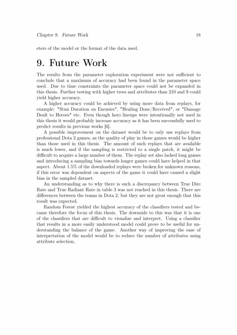
9. Future WorkThe results from the parameter exploration experiment were not sufficient toconclude that a maximum of accuracy had been found in the parameter spaceused. Due to time constraints the parameter space could not be expanded inthis thesis. Further testing with higher trees and attributes than 210 and 9 couldyield higher accuracy.

A higher accuracy could be achieved by using more data from replays, forexample: "Stun Duration on Enemies", "Healing Done/Received", or "DamageDealt to Heroes" etc. Even though hero lineups were intentionally not used inthis thesis it would probably increase accuracy as it has been successfully used topredict results in previous works [6].

A possible improvement on the dataset would be to only use replays fromprofessional Dota 2 games, as the quality of play in those games would be higherthan those used in this thesis. The amount of such replays that are availableis much lower, and if the sampling is restricted to a single patch, it might bedifficult to acquire a large number of them. The replay set also lacked long gamesand introducing a sampling bias towards longer games could have helped in thataspect. About 1.5% of the downloaded replays were broken for unknown reasons,if this error was dependent on aspects of the game it could have caused a slightbias in the sampled dataset.

An understanding as to why there is such a discrepancy between True DireRate and True Radiant Rate in table 3 was not reached in this thesis. There aredifferences between the teams in Dota 2, but they are not great enough that thisresult was expected.

Random Forest yielded the highest accuracy of the classifiers tested and be-came therefore the focus of this thesis. The downside to this was that it is oneof the classifiers that are difficult to visualize and interpret. Using a classifierthat results in a more easily understood model could prove to be useful for un-derstanding the balance of the game. Another way of improving the ease ofinterpretation of the model would be to reduce the number of attributes usingattribute selection.

References

[1] A. Perea, Rationality in Extensive Form Games, 6th ed. Springer, 2001.

[2] R. Aumann and S. Hart, Handbook of Game Theory with Economic Appli-cations, 1st ed. Elsevier, 1992, vol. 1.

[3] R. Bellman, “On the application of dynamic programing to the determinationof optimal play in chess and checkers,” Proceedings of the National Academyof Sciences of the United States of America, vol. 53, no. 2, p. 244, 1965.

[4] A. Joseph, N. E. Fenton, and M. Neil, “Predicting football results usingbayesian nets and other machine learning techniques,” Knowledge-Based Sys-tems, vol. 19, no. 7, pp. 544–553, 2006.

[5] G. Synnaeve and P. Bessière., “A bayesian model for plan recognition in rtsgames applied to starcraft,” in Artificial Intelligence and Interactive DigitalEntertainment, 2011.

[6] K. Conley and D. Perry, “How does he saw me? a recommendation enginefor picking heroes in dota 2,” 2013.

[7] P. Yang, B. Harrison, and D. L. Roberts, “Identifying patterns in combatthat are predictive of success in moba games,” in Proceedings of the 9thInternational Conference on the Foundations of Digital Games, 2014.

[8] M. Mohri, A. Rostamizadeh, and A. Talwalkar, Foundations of MachineLearning. MIT press, 2012.

[9] L. Breiman, “Random forests,” Machine learning, vol. 45, no. 1, pp. 5–32,2001.

[10] R. Kohavi, “A study of cross-validation and bootstrap for accuracy estima-tion and model selection,” in International Joint Conference on ArtificialIntelligence, vol. 14, no. 2, 1995, pp. 1137–1145.

[11] D. M. Powers, “Evaluation: from precision, recall and f-measure to ROC,informedness, markedness and correlation,” Journal of Machine LearningTechnologies, vol. 2, no. 1, pp. 37–63, 2011.

19

References 20

[12] K. Pearson, “X. on the criterion that a given system of deviations from theprobable in the case of a correlated system of variables is such that it canbe reasonably supposed to have arisen from random sampling,” The Lon-don, Edinburgh, and Dublin Philosophical Magazine and Journal of Science,vol. 50, no. 302, pp. 157–175, 1900.

[13] R. A. Fisher, “On the "probable error" of a coefficient of correlation deducedfrom a small sample,” Metron, vol. 1, pp. 3–32, 1921.

[14] D. C. Montgomery, Design and analysis of experiments, 8th ed. John Wiley& Sons, 2012.

[15] B. S. Everitt, The Cambridge dictionary of statistics. Cambridge UniversityPress, 2002.

[16] S. Abu-Nimeh, D. Nappa, X. Wang, and S. Nair, “A comparison of ma-chine learning techniques for phishing detection,” in Proceedings of the anti-phishing working groups 2nd annual eCrime researchers summit, 2007, pp.60–69.

[17] R. Caruana and A. Niculescu-Mizil, “An empirical comparison of supervisedlearning algorithms,” in Proceedings of the 23rd international conference onMachine learning, 2006, pp. 161–168.

[18] R. Caruana, N. Karampatziakis, and A. Yessenalina, “An empirical evalua-tion of supervised learning in high dimensions,” in Proceedings of the 25thinternational conference on Machine learning, 2008, pp. 96–103.

[19] B. Efron, “Bootstrap methods: another look at the jackknife,” The annals ofStatistics, pp. 1–26, 1979.

[20] L. Breiman, “Bagging predictors,” Machine learning, vol. 24, no. 2, pp. 123–140, 1996.

[21] C.-C. Chang and C.-J. Lin, “Libsvm: a library for support vector machines,”ACM Transactions on Intelligent Systems and Technology (TIST), vol. 2,no. 3, p. 27, 2011.

[22] C. Cortes and V. Vapnik, “Support-vector networks,” Machine learning,vol. 20, no. 3, pp. 273–297, 1995.

[23] D. Meyer, F. Leisch, and K. Hornik, “The support vector machine undertest,” Neurocomputing, vol. 55, no. 1, pp. 169–186, 2003.

[24] G. H. John and P. Langley, “Estimating continuous distributions in bayesianclassifiers,” in Proceedings of the Eleventh conference on Uncertainty in ar-tificial intelligence, 1995, pp. 338–345.

References 21

[25] I. Rish, “An empirical study of the naive bayes classifier,” in InternationalJoint Conference on Artificial Intelligence workshop on empirical methods inartificial intelligence, vol. 3, no. 22, 2001, pp. 41–46.

[26] R. E. Schapire, “The strength of weak learnability,” Machine learning, vol. 5,no. 2, pp. 197–227, 1990.

[27] J. Friedman, T. Hastie, and R. Tibshirani, “Additive logistic regression: astatistical view of boosting (with discussion and a rejoinder by the authors),”The annals of statistics, vol. 28, no. 2, pp. 337–407, 2000.

[28] R. A. McDonald, D. J. Hand, and I. A. Eckley, “An empirical comparisonof three boosting algorithms on real data sets with artificial class noise,” inMultiple Classifier Systems, 2003, pp. 35–44.

[29] Y. Freund and R. E. Schapire, “A desicion-theoretic generalization of on-line learning and an application to boosting,” in Proceedings of the SecondEuropean Conference on Computational Learning Theory, 1995, pp. 23–37.

[30] B. Martin, “Instance-based learning: nearest neighbour with generalisation,”Master’s thesis, University of Waikato, 1995.

[31] B. G. Weber and M. Mateas, “A data mining approach to strategy predic-tion,” in IEEE Conference on Computational Intelligence and Games, 2009,pp. 140–147.

[32] T. Fawcett, “An introduction to ROC analysis,” Pattern Recognition Letters,vol. 27, no. 8, pp. 861–874, 2006.

[33] S. S. Shapiro and M. B. Wilk, “An analysis of variance test for normality(complete samples),” Biometrika, vol. 52, no. 3/4, pp. 591–611, 1965.

[34] I. Olkin, Contributions to probability and statistics: essays in honor of HaroldHotelling. Stanford University Press, 1960.

A. Raw Data FormatThe format of the file is WEKAs ARFF format1, and the data consists of 177attributes. Every attribute is team based so data that is player specific is summedfor all players on that team. With the exception of MatchID, GameTime, andWinner all attributes are paired, one for each team. For example, player killsare recorded in two variables, Kills_radiant and Kills_dire. The entirety of theformat consists of the following attribute sets for each team: kills, deaths, assists,last hits, denies, runes used, net worth, tower kills, barracks destroyed, ancient hp,roshan kills, and 76 attributes of items constructed from recipes. The majorityof items that are purchased without being built from recipes are usually acquiredonly to eventually finish a recipe or sell later, and are therefore not as indicativeof item progression and omitted from the format. MatchID is only used whenconstructing subsets of the instances, and removed before used in training orvalidation of models.

B. TeamAdvantage FormatTeamAdvatange is a reparsing of the raw data file where every pair of attributesrelated to the teams gets converted to a single attribute with the possible valuesof Radiant, Dire, Initial, or Tie. It will either be Radiant or Dire if one of thoseteams is in the lead, otherwise it will be initial if the attributes are unchanged ortie if both teams are equal.

Example raw data: @attribute Kills_radiant integer, @attribute Kills_direinteger. Gets converted into: @attribute KillsLeader Radiant, Dire, Initial, Tie.

C. Valve API usageThe url used was:https://api.steampowered.com/IDOTA2Match_570/GetMatchHistory/V001/?key=<key>&skill=3&min_players=10&game_mode=1In this URL the <key> is personal value which is acquired after accepting Valve’sTOS2, "skill=3" is used to filter to very high skill games, "min_players=10" isused to filter out games where the teams are not completely full and "game_mode=1"is used to filter so the games retrieve are of the game mode "All Pick".

1http://weka.wikispaces.com/ARFF Accessed: 6-1-20152http://steamcommunity.com/dev/apiterms Accessed: 6-1-2015

A

D. Computer Specifications used fortime measurementsThe computer used for the time measurements can be seen below:

CPU AMD Turion II Dual-Core 64 bit 2 MB, 2.2GHzMemory Kingston 16GB 1333MHz DDR3 ECC CL9Harddrive 250 GB, 7200 RPM, SATAOperating System FreeBSD

E. List of Average Game Lengths ofValidation SetsThe table presents a list of all average game lengths from 125 generated validationsets in minutes.

22.45 22.74 22.63 22.61 22.5922.56 22.42 22.59 22.90 22.7622.47 22.48 22.70 22.77 22.7322.78 22.49 22.48 22.80 22.7322.63 22.79 22.62 22.60 22.7922.55 22.51 22.69 22.76 22.5822.64 22.55 22.62 22.65 22.8422.57 22.51 22.52 22.74 22.7622.46 22.75 22.65 22.62 22.6922.63 22.75 22.65 22.69 22.7822.72 22.52 22.56 22.66 22.7122.74 22.76 22.67 22.70 22.5222.69 22.65 22.55 22.72 22.6622.70 22.84 22.58 22.61 22.6822.36 22.68 22.47 22.71 22.5122.68 22.43 22.55 22.69 22.8322.54 22.63 22.55 22.82 22.5322.65 22.57 22.67 22.34 22.7022.55 23.00 22.77 22.72 22.4822.56 22.65 22.54 22.43 22.7522.41 22.68 22.56 22.72 22.7522.46 22.63 22.60 22.66 22.6222.59 22.61 22.87 22.50 22.6722.76 22.45 22.77 22.41 22.5522.73 22.71 22.62 22.66 22.42

Table 7: Average Game Length of Validation Sets

B

F. Random Forest Per MinuteSummary

Default Parameters Majority Class Random Forest 210 trees, 9 attributesGT Inst. Acc. TRR TDR0 15004 53.29% 68.38% 32.66%1 14988 60.63% 78.14% 36.71%2 14983 66.78% 81.04% 47.28%3 14956 71.77% 83.51% 55.72%4 14852 76.38% 86.24% 62.84%5 14732 78.90% 87.75% 66.75%6 14584 81.79% 89.25% 71.50%7 14457 84.44% 90.97% 75.43%8 14278 86.20% 91.61% 78.75%9 14051 88.08% 92.94% 81.34%10 13778 89.98% 93.91% 84.53%11 13497 91.41% 94.58% 87.01%12 13206 92.37% 95.49% 88.02%13 12867 93.67% 96.27% 90.00%14 12571 95.05% 97.27% 91.90%15 12239 95.59% 97.47% 92.89%16 11978 96.39% 98.11% 93.90%17 11689 96.97% 98.12% 95.29%18 11336 97.62% 98.59% 96.20%19 10970 97.99% 98.87% 96.69%20 10560 98.29% 98.88% 97.40%21 10126 98.71% 99.03% 98.23%22 9616 98.89% 99.22% 98.39%23 8973 99.15% 99.50% 98.63%24 8184 99.55% 99.73% 99.27%25 7424 99.54% 99.64% 99.41%26 6606 99.56% 99.61% 99.49%27 5610 99.57% 99.66% 99.45%28 4669 99.76% 99.85% 99.64%29 3753 99.89% 99.95% 99.81%30 2864 99.86% 99.88% 99.84%31 2089 99.86% 99.91% 99.78%32 1435 99.79% 100.00% 99.55%33 978 99.80% 100.00% 99.57%34 670 99.85% 100.00% 99.69%35 387 99.48% 100.00% 98.97%36 242 99.17% 100.00% 98.21%37 151 98.68% 100.00% 97.33%38 85 97.65% 100.00% 94.59%39 40 95.00% 100.00% 84.62%40 18 88.89% 100.00% 66.67%41 11 81.82% 100.00% 60.00%42 10 80.00% 100.00% 50.00%43 8 75.00% 100.00% 33.33%44 8 75.00% 100.00% 33.33%45 2 100.00% 100.00% 100.00%46 2 100.00% 100.00% 100.00%47 2 100.00% 100.00% 100.00%

GT Inst. Acc. TRR TDR0 15132 58.91% 58.91% 0.00%1 15117 58.90% 58.90% 0.00%2 15100 58.90% 58.90% 0.00%3 15057 58.97% 58.97% 0.00%4 14957 58.99% 58.99% 0.00%5 14836 58.96% 58.96% 0.00%6 14681 59.16% 59.16% 0.00%7 14558 59.23% 59.23% 0.00%8 14356 59.21% 59.21% 0.00%9 14129 59.32% 59.32% 0.00%10 13856 59.45% 59.45% 0.00%11 13599 59.53% 59.53% 0.00%12 13295 59.78% 59.78% 0.00%13 12961 60.03% 60.03% 0.00%14 12663 60.21% 60.21% 0.00%15 12334 60.40% 60.40% 0.00%16 12064 60.57% 60.57% 0.00%17 11748 60.91% 60.91% 0.00%18 11431 61.20% 61.20% 0.00%19 11099 61.51% 61.51% 0.00%20 10663 61.73% 61.73% 0.00%21 10231 61.86% 61.86% 0.00%22 9703 62.02% 62.02% 0.00%23 9074 62.00% 62.00% 0.00%24 8275 61.89% 61.89% 0.00%25 7461 61.39% 61.39% 0.00%26 6630 61.10% 61.10% 0.00%27 5651 60.31% 60.31% 0.00%28 4652 60.04% 60.04% 0.00%29 3735 59.14% 59.14% 0.00%30 2871 58.76% 58.76% 0.00%31 2072 59.46% 59.46% 0.00%32 1421 58.13% 58.13% 0.00%33 973 56.01% 56.01% 0.00%34 666 55.86% 55.86% 0.00%35 374 53.21% 53.21% 0.00%36 245 57.55% 57.55% 0.00%37 137 61.31% 61.31% 0.00%38 86 63.95% 63.95% 0.00%39 41 78.05% 78.05% 0.00%40 21 85.71% 85.71% 0.00%41 14 78.57% 78.57% 0.00%42 8 62.50% 62.50% 0.00%43 4 25.00% 25.00% 0.00%44 3 33.33% 33.33% 0.00%45 0 NA NA 0.00%46 0 NA NA 0.00%47 0 NA NA 0.00%

GT Inst. Acc. TRR TDR0 15231 53.44% 65.53% 36.79%1 15219 63.14% 78.48% 42.03%2 15209 69.45% 79.19% 56.06%3 15181 74.58% 82.24% 64.02%4 15073 79.15% 85.31% 70.62%5 14943 82.23% 87.26% 75.28%6 14793 84.68% 89.17% 78.44%7 14658 86.84% 90.51% 81.74%8 14464 88.52% 91.56% 84.33%9 14238 90.53% 92.66% 87.56%10 13937 91.66% 93.55% 89.00%11 13636 93.05% 94.56% 90.92%12 13313 94.10% 95.60% 91.98%13 12977 94.99% 96.23% 93.23%14 12709 95.95% 97.01% 94.42%15 12380 96.70% 97.37% 95.72%16 12085 97.28% 98.03% 96.18%17 11781 97.89% 98.52% 96.98%18 11457 98.21% 98.69% 97.50%19 11098 98.52% 98.92% 97.92%20 10659 98.80% 99.07% 98.39%21 10193 99.00% 99.22% 98.66%22 9684 99.14% 99.32% 98.87%23 9064 99.39% 99.53% 99.18%24 8293 99.49% 99.60% 99.33%25 7505 99.44% 99.53% 99.30%26 6659 99.62% 99.70% 99.51%27 5703 99.67% 99.68% 99.65%28 4661 99.74% 99.71% 99.79%29 3763 99.76% 99.77% 99.75%30 2861 99.69% 99.75% 99.59%31 2067 99.85% 100.00% 99.67%32 1392 99.93% 100.00% 99.84%33 949 99.89% 100.00% 99.77%34 643 99.84% 100.00% 99.67%35 380 99.74% 100.00% 99.43%36 248 99.60% 100.00% 99.11%37 160 99.38% 100.00% 98.59%38 98 98.98% 100.00% 97.44%39 50 98.00% 100.00% 94.74%40 25 96.00% 100.00% 87.50%41 19 94.74% 100.00% 83.33%42 12 91.67% 100.00% 83.33%43 8 87.50% 100.00% 80.00%44 5 100.00% 100.00% 100.00%45 1 100.00% NA 100.00%46 1 100.00% NA 100.00%47 1 100.00% NA 100.00%

Table 8: Summary of Random Forest classifier per minute with different param-eters

C