This is a preprint of a paper intended for publication in a journal or proceedings. Since changes may be made before publication, this preprint should not be cited or reproduced without permission of the author. This document was prepared as an account of work sponsored by an agency of the United States Government. Neither the United States Government nor any agency thereof, or any of their employees, makes any warranty, expressed or implied, or assumes any legal liability or responsibility for any third party’s use, or the results of such use, of any information, apparatus, product or process disclosed in this report, or represents that its use by such third party would not infringe privately owned rights. The views expressed in this paper are not necessarily those of the United States Government or the sponsoring agency.

INL/CON-14-31971PREPRINT

Resilient Control Systems Practical Metrics Basis for Defining Mission Impact

Resilience Week

Craig G. Rieger

August 2014

1

Resilient Control Systems Practical Metrics Basis for Defining Mission Impact

Craig G. Rieger Senior Member, IEEE

Idaho National Laboratory Idaho Falls, Idaho, USA

Abstract—“Resilience” describes how systems operate at an acceptable level of normalcy despite disturbances or threats. In this paper we first consider the cognitive, cyber-physical interdependencies inherent in critical infrastructure systems and how resilience differs from reliability to mitigate these risks. Terminology and metrics basis are provided to integrate the cognitive, cyber-physical aspects that should be considered when defining solutions for resilience. A practical approach is taken to roll this metrics basis up to system integrity and business case metrics that establish “proper operation” and “impact.” A notional chemical processing plant is the use case for demonstrating how the system integrity metrics can be applied to establish performance, and as well, the effects on the process that roll into the business case.

Keywords—Metrics, cogntive, cyber-physical, adaptive capacity, adaptive insufficience, resilience, robustness, performance, threats.

I. INTRODUCTION

A. Critical Infrastructure Systems Hurricane Sandy bluntly reminded us how we take for granted the complex systems that provide energy, transportation, water, medical care, emergency response, and security at levels considered luxurious just a generation ago. Presidential Policy Directive 21 (PPD-21), “Critical Infrastructure Security and Resilience” recognized the need to advance research and development (R&D) for resilient critical infrastructure. At the core of critical infrastructure operation are control systems. However, unlike the highly autonomous characterizations of control systems believed by many to be at the heart of efficient, effective and resilient critical infrastructure systems, modern control systems are effectively digital versions of the analog systems they replaced. While these networked platforms have provided a means to establish central monitoring and ease integration of feedback controls, the algorithms used are primarily the same as those invented prior to 1950. Unfortunately, the ability to network distributed components has established a framework for additional cyber, cognitive and human complex interdependencies and a resulting system rigidity or brittleness, establishing the potential for cascading failures. Current control systems lack the ability to analyze failures of the critical infrastructure system controlled, or even sensors and field devices, and require the operator/dispatcher to be the analyst and root cause expert mining the large volume of data received. Ultimately, modern control systems lack the framework needed to achieve global production efficiencies, let alone the ability to recognize and optimize a response to a natural or manmade malicious or benign, unintended event, and therefore is a fundamental gap to establishing resilient critical infrastructure

systems. Without a significant investment by the federal government to address this national gap in technology, policies and regulations, modern control systems will remain the soft underbelly for cyber-attacks, a major impediment to implementing national Smart Grid, and the limiting technology to optimizing response to the next national emergency like the Hurricane Sandy.

B. Resilient Control Systems The following is adapted from [1], which provides the definition:

A resilient control system is one that maintains state awareness and an accepted level of operational normalcy in response to disturbances, including threats of an unexpected and malicious nature

The “resilient control system” (RCS) is arguably a new control design paradigm that encompasses cybersecurity, physical security, economic efficiency, dynamic stability, and process compliancy in large-scale, complex systems. From a conventional control engineering perspective one might say that an RCS is merely dependable computing coupled with fault tolerant control, however, we argue [2] that this perspective is too narrow. For example, while the fault tolerant control community has developed ideas of fault detection and identification and to some extent the ideas of reconfiguration, these are not readily linked to control response; nor does the control community have a way yet to systematically consider faults resulting from the cyber-environment associated with the system. RCS attempts to synergistically capture both the cyber and the physical aspects of system design and operation, thereby overcoming the limitations of the reliable computing and fault tolerant control perspective.

Research and development (R&D) and associated international symposia have developed the technological perspectives and definition of RCS [3]. It is now timely to establish a means to evaluate technology investment into R&D that will mature technologies into industrial and military applications. In addition, as a ground truth for impacts from manmade and natural events, a method to correlate operational awareness is required. In line with these needs, metrics are necessary to establish the following:

• System Integrity, Which Establishes Ongoing System Run-Time Performance

• Business Case for Resilience, Which Establishes the Value Proposition Based Upon Desired Performance

Both of these is important in its own right, and will be the subject of this paper.

C. Paper Outline In the foregoing, we discussed the need for a new control engineering paradigm that we term “resilient control systems” as a means of moving beyond conventional control engineering. To establish metrics for the ongoing R&D and standards community activities, this paper will provide a metrics framework and use cases that integrate the diverse aspects of resilience. To provide a perspective on how resilience differs from reliability, Section II provides an overview of accepted considerations [2]. Section III then establishes alternative frameworks for the two metrics types. Section IV applies these frameworks to note use cases. Section V provides system integrity and business case metrics based upon the metrics basis. Section VI provides a step-by-step metrics process, with a quantitative example in Section VII for a notional chemical processing plant.. Finally, Section VII provides a concept for presentation of system integrity metrics.

II. RESILIENCE VERSUS RELIABILITY The next generation of control systems should have a threat-based approach to develop control systems that are resilient by nature. As such, the ability to not only detect, but correlate the impact on the ability to achieve minimum normalcy is a necessary attribute. Unlike fault tolerance approaches, what follows are ill-defined interdependencies that distinguish resilience from reliability [2].

• Unexpected condition adaptation o Achievable hierarchy with semi-autonomous echelons:

The ability to have large scale, integrated supervisory control methodologies that implement graceful degradation.

o Complex interdependencies and latency: Widely distributed, dynamic control system elements organized to prevent destabilization of controlled system.

• Human interaction challenges o Human performance prediction: Humans possess great

capability based upon knowledge and skill, but are not always operating at the same performance level.

o Cyber awareness and intelligent adversary: The ability to mitigate cyber-attacks is necessary to ensure the integrity of the control system.

• Goal conflicts o Multiple performance goals: Besides stability,

security, efficiency and other factors influence the overall criteria for performance of the control system.

o Lack of state awareness: Raw data must be translated to information on the condition of the process and the control system components.

Establishing metrics for resilience requires reflection on these characteristics. Three common, potentially destabilizing dynamical aspects will in particular be used to establish use

cases in resilience. These include control system operation, cyber system security and human system interaction. First to lay the groundwork, the base metrics will be discussed in the next section and lay out the overall design that can be implemented in the use cases.

III. METRICS BASIS Establishing a metric that can capture the resilience attributes can be complex, at least if considered based upon differences between the interactions or interdependencies. Evaluating the control, cyber and cognitive disturbances, especially if considered from a disciplinary standpoint, leads to measures that already been established. However, if the metric were instead based upon a normalizing dynamic attribute, such a performance characteristic that can be impacted by degradation, an alternative is suggested. Specifically, applications of base metrics to resilience characteristics are given as follows for type of disturbance:

• Physical Disturbances: o Time Latency Affecting Stability o Data Integrity Affecting Stability

• Cyber Disturbances: o Time Latency o Data Confidentiality, Integrity and Availability

• Cognitive Disturbances: o Time Latency in Response o Data Digression from Desired Response

Such performance characteristics exist with both time and data integrity. Time, both in terms of delay of mission and communications latency, and data, in terms of corruption or modification, are normalizing factors. In general, the idea is to base the metric on “what is expected” and not necessarily the actual initiator to the degradation. Considering time as a metrics basis, resilient and un-resilient systems can be observed in Fig. 1 [4].

Dependent upon the abscissa metrics chosen, Fig. 1 reflects a generalization of the resiliency of a system. Several common terms are represented on this graphic, including robustness, agility, adaptive capacity, adaptive insufficiency, resiliency and brittleness. To overview the definitions of these terms, the following explanations of each is provided below:

• Agility: The derivative of the disturbance curve. This average defines the ability of the system to resist degradation on the downward slope, but also to recover on the upward. Primarily considered a time based term that indicates impact to mission.

• Adaptive Capacity: The ability of the system to adapt or transform from impact and maintain minimum normalcy. Considered a value between 0 and 1, where 1 is fully operational and 0 is the resilience threshold.

• Adaptive Insufficiency: The inability of the system to adapt or transform from impact, indicating an unacceptable performance loss due to the disturbance. Considered a value between 0 and -1, where 0 is the resilience threshold and -1 is total loss of operation.

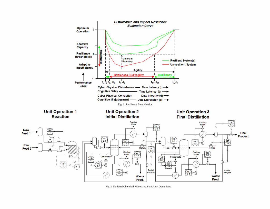
Fig. 1. Resilience Base Metrics

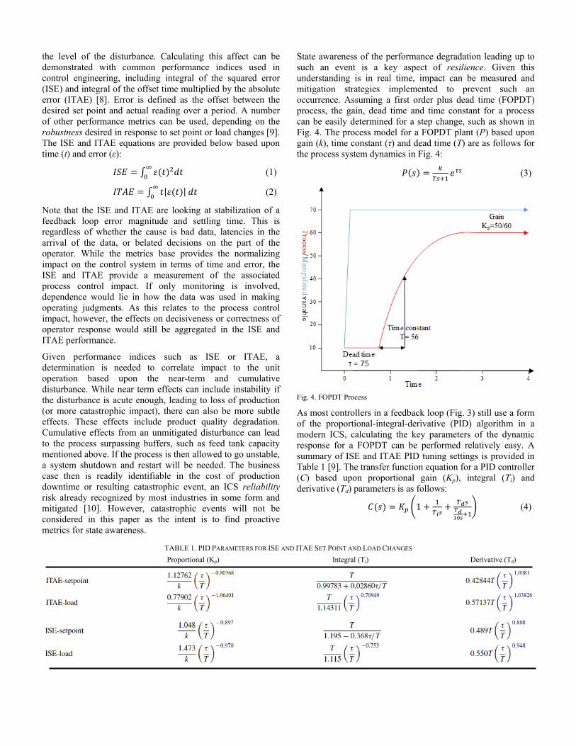
Fig. 2. Notional Chemical Processing Plant Unit Operations

• Brittleness: The area under the disturbance curve as intersected by the resilience threshold. This indicates the impact from the loss of operational normalcy.

• Resiliency: The converse of brittleness, which for a resilience system is “zero” loss of minimum normalcy.

• Robustness: A positive or negative number associated with the area between the disturbance curve and the resilience threshold, indicating either the capacity or insufficiency, respectively.

On the abscissa of Fig. 1, it can be recognized that cyber and cognitive influences can affect both the data and the time, which underscores the relative importance of recognizing these forms of degradation in resilient control designs. For cyber security, a single cyber-attack can degrade a control system in multiple ways. Additionally, control impacts can be characterized as indicated. While these terms are fundamental and seem of little value for those correlating impact in terms like cost, the development of use cases provide a means by which this relevance can be codified. For the purposes of this paper, we shall prescribe a uses case that covers the earlier mentioned metrics of business case and system integrity.

IV. METRICS USE CASE To establish a use case for metrics, a critical infrastructure of a chemical processing plant is chosen and that plant is decomposed into the functional dynamic elements or agents [5]. That is, operational elements are associated with unit operations or some optimally stabilizable entity. The unit operation, in this case, defines an area of local optimization. Within the operation, many physical variables may exist. In a plant made up of many unit operations, such as in Fig. 2, the process of determining the optimally stabilizable entities normally results in a minimization of the interactions between individual unit operations. That is, normally only a few physical variables will make up the interactions between unit operations. For example, the flow and thermodynamic characteristics of steam to the reboiler or cooling water to the condenser must remain within a specified range to maintain distillation column equilibrium. This is also important to the stability of the downstream operation as it is expecting flow to remain within a designed range, too high leading to overflows and too low leading to inadequate feed.

The control theory applied to achieving stability within a unit operation comes in the form of feedback loops, such as that indicated in Fig. 3. The types of dynamics that can make up any feedback loop in this chemical process can include several networked modules and microprocessor calculations and conversions. As a result, measurements, control algorithms and actions may be hosted on distributed devices that are interconnected with communications networks, creating what is considered a networked control system [6].

However, Fig. 2 only represents the dynamics of control. In order to correctly interpret resilience dynamics in the form of Fig. 1, the control, cyber and cognitive dynamics must be broken down into a more appropriate agent design. Take for example the Resilient Control System Execution Agent

(ReCoSEA), which is a cyber-physical agent that senses its environment and acts upon it [7]. Disturbances consider both the cyber and physical aspects as impacts to the control system performance, and the human is a necessary attribute in the feedback response that can also impact performance. Disturbances to the control system exhibit impacts in the form of time and data as characterized in Fig. 1.

Fig. 3. Process Feedback Loop

Reflecting the strategy of ReCoSEA and considering the base metrics of Fig. 1, the effects of disturbances can be associated with cyber, physical and human causes. Time impacts that are reflected through destabilizing latencies may be the result of cyber-attacks or cognitive interactions. Toward the former, latencies are created in ICS communications, either through a security compromise effect (e.g., denial of service), or physical degradation of control system components. Cognitive latencies involve the decision process of a human and delayed response to disturbances in interfacing to the ICS and the plant it controls. Data impacts may be reflected through integrity compromises resulting from cyber-attacks. An undesirable decision from the human for the particular circumstances can lead to a digression of the plant to suboptimal or destabilizing outcomes.

With these base metrics, the following section develop a methodology to a business case and system integrity metrics design.

V. SYSTEM INTEGRITY AND BUSINESS CASE METRICS Scaling up the base metrics to an overall mission impact requires a process operation to establish relevance, which for this paper is a chemical processing plant. Application of the base metrics first requires the correlation of disturbances to the several unit operations that make up a chemical processing plant. However, while the individual impact to the business by each unit operation can vary, calculation of the effects within the ICS is not dependent upon this characteristic. Therefore, if the base metrics can correlated for the disturbance, how this impacts the unit operation is simply the application of how the disturbance impacts efficiency and stability.

As a notional example to shape a metrics design, let’s assume a distillation column in a chemical processing plant has three controllers associated with the feed tank, reboiler and condenser in Unit Operation 2 of Fig. 2. Dependent upon the effects of a disturbance on any or all of these controllers, the stability of this unit operation and the upstream/downstream unit operations may be affected. Head tanks at the feed to Unit Operation 2 and also downstream provide some buffering to variations in flow. The affect to normalcy will depend upon

the level of the disturbance. Calculating this affect can be demonstrated with common performance indices used in control engineering, including integral of the squared error (ISE) and integral of the offset time multiplied by the absolute error (ITAE) [8]. Error is defined as the offset between the desired set point and actual reading over a period. A number of other performance metrics can be used, depending on the robustness desired in response to set point or load changes [9]. The ISE and ITAE equations are provided below based upon time (t) and error (ε):

𝐼𝑆𝐸 = ∫ 𝜀(𝑡)2𝑑𝑡∞0 (1)

𝐼𝑇𝐴𝐸 = ∫ 𝑡|𝜀(𝑡)| 𝑑𝑡∞0 (2)

Note that the ISE and ITAE are looking at stabilization of a feedback loop error magnitude and settling time. This is regardless of whether the cause is bad data, latencies in the arrival of the data, or belated decisions on the part of the operator. While the metrics base provides the normalizing impact on the control system in terms of time and error, the ISE and ITAE provide a measurement of the associated process control impact. If only monitoring is involved, dependence would lie in how the data was used in making operating judgments. As this relates to the process control impact, however, the effects on decisiveness or correctness of operator response would still be aggregated in the ISE and ITAE performance.

Given performance indices such as ISE or ITAE, a determination is needed to correlate impact to the unit operation based upon the near-term and cumulative disturbance. While near term effects can include instability if the disturbance is acute enough, leading to loss of production (or more catastrophic impact), there can also be more subtle effects. These effects include product quality degradation. Cumulative effects from an unmitigated disturbance can lead to the process surpassing buffers, such as feed tank capacity mentioned above. If the process is then allowed to go unstable, a system shutdown and restart will be needed. The business case then is readily identifiable in the cost of production downtime or resulting catastrophic event, an ICS reliability risk already recognized by most industries in some form and mitigated [10]. However, catastrophic events will not be considered in this paper as the intent is to find proactive metrics for state awareness.

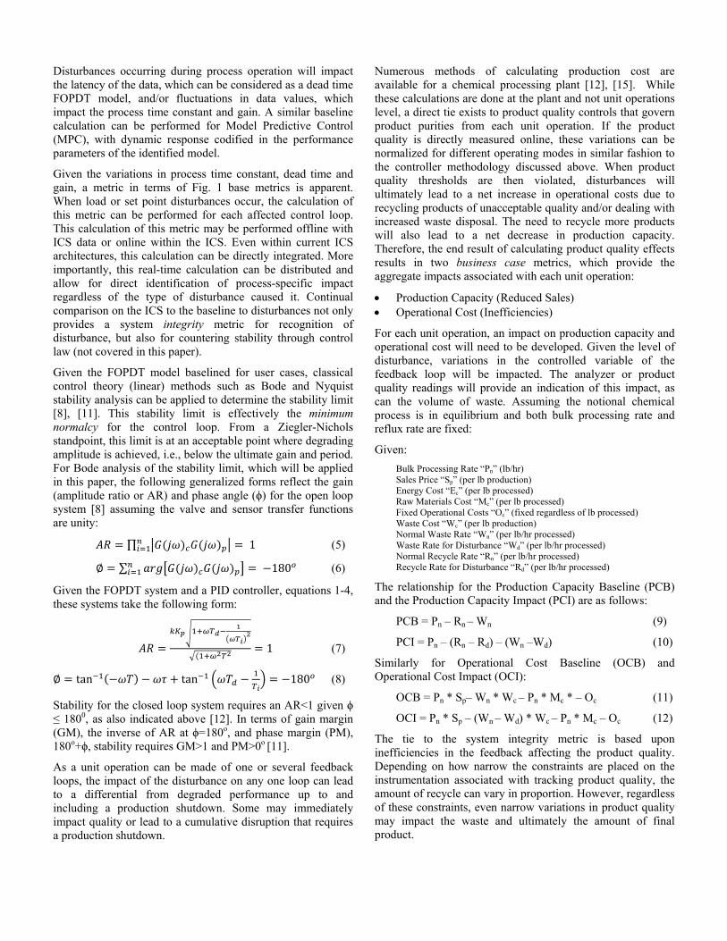
State awareness of the performance degradation leading up to such an event is a key aspect of resilience. Given this understanding is in real time, impact can be measured and mitigation strategies implemented to prevent such an occurrence. Assuming a first order plus dead time (FOPDT) process, the gain, dead time and time constant for a process can be easily determined for a step change, such as shown in Fig. 4. The process model for a FOPDT plant (P) based upon gain (k), time constant (τ) and dead time (T) are as follows for the process system dynamics in Fig. 4:

𝑃(𝑠) = 𝑘𝑇𝑠+1

𝑒𝜏𝑠 (3)

Fig. 4. FOPDT Process

As most controllers in a feedback loop (Fig. 3) still use a form of the proportional-integral-derivative (PID) algorithm in a modern ICS, calculating the key parameters of the dynamic response for a FOPDT can be performed relatively easy. A summary of ISE and ITAE PID tuning settings is provided in Table 1 [9]. The transfer function equation for a PID controller (C) based upon proportional gain (Kp), integral (Ti) and derivative (Td) parameters is as follows:

𝐶(𝑠) = 𝐾𝑝 �1 + 1𝑇𝑖𝑠

+ 𝑇𝑑𝑠𝑇𝑑10𝑠+1

� (4)

TABLE 1. PID PARAMETERS FOR ISE AND ITAE SET POINT AND LOAD CHANGES Proportional (Kp) Integral (Ti) Derivative (Td)

Disturbances occurring during process operation will impact the latency of the data, which can be considered as a dead time FOPDT model, and/or fluctuations in data values, which impact the process time constant and gain. A similar baseline calculation can be performed for Model Predictive Control (MPC), with dynamic response codified in the performance parameters of the identified model.

Given the variations in process time constant, dead time and gain, a metric in terms of Fig. 1 base metrics is apparent. When load or set point disturbances occur, the calculation of this metric can be performed for each affected control loop. This calculation of this metric may be performed offline with ICS data or online within the ICS. Even within current ICS architectures, this calculation can be directly integrated. More importantly, this real-time calculation can be distributed and allow for direct identification of process-specific impact regardless of the type of disturbance caused it. Continual comparison on the ICS to the baseline to disturbances not only provides a system integrity metric for recognition of disturbance, but also for countering stability through control law (not covered in this paper).

Given the FOPDT model baselined for user cases, classical control theory (linear) methods such as Bode and Nyquist stability analysis can be applied to determine the stability limit [8], [11]. This stability limit is effectively the minimum normalcy for the control loop. From a Ziegler-Nichols standpoint, this limit is at an acceptable point where degrading amplitude is achieved, i.e., below the ultimate gain and period. For Bode analysis of the stability limit, which will be applied in this paper, the following generalized forms reflect the gain (amplitude ratio or AR) and phase angle (ϕ) for the open loop system [8] assuming the valve and sensor transfer functions are unity:

𝐴𝑅 = ∏ �𝐺(𝑗𝜔)𝑐𝐺(𝑗𝜔)𝑝�𝑛𝑖=1 = 1 (5)

∅ = ∑ 𝑎𝑟𝑔�𝐺(𝑗𝜔)𝑐𝐺(𝑗𝜔)𝑝� = −180𝑜𝑛𝑖=1 (6)

Given the FOPDT system and a PID controller, equations 1-4, these systems take the following form:

𝐴𝑅 =𝑘𝐾𝑝�1+𝜔𝑇𝑑−

1

�𝜔𝑇𝑖�2

�(1+𝜔2𝑇2= 1 (7)

∅ = tan−1(−𝜔𝑇) −𝜔𝜏 + tan−1 �𝜔𝑇𝑑 −1𝑇𝑖� = −180𝑜 (8)

Stability for the closed loop system requires an AR<1 given ϕ ≤ 1800, as also indicated above [12]. In terms of gain margin (GM), the inverse of AR at ϕ=180o, and phase margin (PM), 180o+ϕ, stability requires GM>1 and PM>0o [11].

As a unit operation can be made of one or several feedback loops, the impact of the disturbance on any one loop can lead to a differential from degraded performance up to and including a production shutdown. Some may immediately impact quality or lead to a cumulative disruption that requires a production shutdown.

Numerous methods of calculating production cost are available for a chemical processing plant [12], [15]. While these calculations are done at the plant and not unit operations level, a direct tie exists to product quality controls that govern product purities from each unit operation. If the product quality is directly measured online, these variations can be normalized for different operating modes in similar fashion to the controller methodology discussed above. When product quality thresholds are then violated, disturbances will ultimately lead to a net increase in operational costs due to recycling products of unacceptable quality and/or dealing with increased waste disposal. The need to recycle more products will also lead to a net decrease in production capacity. Therefore, the end result of calculating product quality effects results in two business case metrics, which provide the aggregate impacts associated with each unit operation:

• Production Capacity (Reduced Sales) • Operational Cost (Inefficiencies)

For each unit operation, an impact on production capacity and operational cost will need to be developed. Given the level of disturbance, variations in the controlled variable of the feedback loop will be impacted. The analyzer or product quality readings will provide an indication of this impact, as can the volume of waste. Assuming the notional chemical process is in equilibrium and both bulk processing rate and reflux rate are fixed:

Given: Bulk Processing Rate “Pn” (lb/hr) Sales Price “Sp” (per lb production) Energy Cost “Ec” (per lb processed) Raw Materials Cost “Mc” (per lb processed) Fixed Operational Costs “Oc” (fixed regardless of lb processed) Waste Cost “Wc” (per lb production) Normal Waste Rate “Wn” (per lb/hr processed) Waste Rate for Disturbance “Wd” (per lb/hr processed) Normal Recycle Rate “Rn” (per lb/hr processed) Recycle Rate for Disturbance “Rd” (per lb/hr processed)

The relationship for the Production Capacity Baseline (PCB) and the Production Capacity Impact (PCI) are as follows:

PCB = Pn – Rn – Wn (9)

PCI = Pn – (Rn – Rd) – (Wn –Wd) (10)

Similarly for Operational Cost Baseline (OCB) and Operational Cost Impact (OCI):

OCB = Pn * Sp– Wn * Wc – Pn * Mc * – Oc (11)

OCI = Pn * Sp – (Wn – Wd) * Wc – Pn * Mc – Oc (12)

The tie to the system integrity metric is based upon inefficiencies in the feedback affecting the product quality. Depending on how narrow the constraints are placed on the instrumentation associated with tracking product quality, the amount of recycle can vary in proportion. However, regardless of these constraints, even narrow variations in product quality may impact the waste and ultimately the amount of final product.

Multiple standard fault detection and diagnosis techniques could also be applied to the analyzer data, such as principle product analysis and partial least squares [16]. However, these techniques require an offline design analysis before application to define a statistically significant variable from multivariable data sets. For the chemical processing plant, the benefit would be to recognize those variables that are most impactful to product quality. In this paper the focus is to baseline performance relative to real-time disturbances that can affect any of the active feedback controllers, and as such, are inherently more impactful on process stability. As the source of the disturbance can include cognitive and cyber failure in addition to physical, metrics associated with the feedback controller performance becomes a likely candidate for recognition of these sources.

VI. METRICS DEFINITION SUMMARY The following list summarizes the required steps for developing the system integrity and business case metrics. Note that other performance indices and methods can be used to develop the overall metric within these steps, if the developer has a different indicator of control performance they would prefer to use than ISE and ITAE.

• Step 1: Establish test cases to characterize the boundaries of baseline system response for an individual feedback loop. These test cases include set point and load changes that establish desired response to disturbances.

• Step 2: Follow a normal PID tuning procedure for an individual feedback loop to establish initial PID settings [17]-[19]. Refine tuning settings to desired optimum performance settings by evaluating effects on ISE and ITAE for accepted test cases.

• Step 3: Quantify desired optimum performance thresholds and PID parameters for this baseline system response based upon ISE and ITAE formulae [9]. The minimum normalcy thresholds can then be established in the form of the process gain, time constant and dead time, using equations in Table 1. Any number of available commercial tools can also be used for tuning and fitting the FOPDT [20], [21]. This step quantifies the system integrity metric.

• Step 4: Given the optimum performance thresholds and FOPDT model, quantify the ISE and ITAE limits of stability for the feedback loop. This can be done with the process, while monitoring the ISE and ITAE, or through many well know methods such as those discussed [8], [11]. This threshold is the minimum normalcy.

• Step 5: Quantify production cost and capacity due to effect of disturbance impacts on product quality measurements and waste effluent, up to and including production ceasing [12], [15]. Evaluate the business case by normalizing the operational costs and production capacity to negate variations due only to different acceptable operation modes.

VII. QUANTITATIVE EXAMPLE The following examples will illustrate the use of the metrics development, originating with the development of test cases that establish the baseline for real-time comparison. The notable enhancement from a traditional process control use case will be that the initiator of the disturbance will be described. The first example will be the notional chemical processing plant, a use case that formed the backdrop of the discussion up to this point.

Chemical and control engineers have often heard of benchmark processes such as the Tennessee Eastman. Several recognized disturbances (faults) are reflected in this benchmark [22]. With the notional chemical processing plant of Fig. 2, a similar combination of unit operations is considered, as well as the resulting disturbances.

• Step 1: Individual test cases will be defined below that demonstrate the resilience of the chemical processing plant to cyber-physical and cognitive disturbances types discussed early in the paper. These use cases defined for PI control of Unit Operation #2 are as follows, providing one representative case per disturbance type:

o Physical Disturbance: Time Latency Affecting Stability: An IT

technician changes the settings for a switch on the control system network, leading to a slowdown of network traffic and inability to receive timely updates between the human machine interfaces and the controller for this process. As a result, a change in the fractionators level set point that was too drastic was not able to be corrected until the product quality was affected.

Data Integrity Affecting Stability: A gradual degradation in a level transmitter is leading to the associated feedback controller gradually decreasing the level of the fractionator without alarm recognition and impacting quality.

o Cyber Disturbance: Time Latency: A Denial-of-Service attack is

directed toward an ICS device. All of the controllers are affected, causing widespread affects and potential instability.

Data Confidentiality, Integrity and Availability: A man-in-the-middle attack is created that spoofs data to an operator interface unit, implying that that the feed rate is too low, causing the operator to increase feed. Impact to desired product quality is immediate.

o Cognitive Disturbance: Time Latency in Response: Due to multiple

alarms, operator fails to respond in time to a low feed rate. Impact to desired product quality is immediate.

Data Digression from Desired Response: Due to misinterpretation, an operator incorrectly adjusts

the feed during the startup phases of operation. As this column has few trays, the effect on the product is immediately noted.

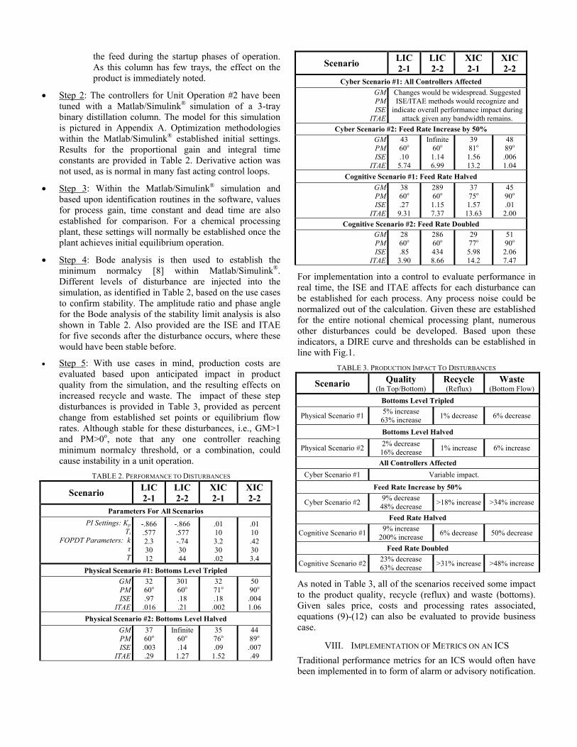
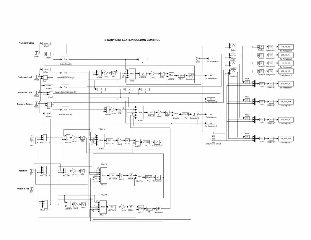
• Step 2: The controllers for Unit Operation #2 have been tuned with a Matlab/Simulink® simulation of a 3-tray binary distillation column. The model for this simulation is pictured in Appendix A. Optimization methodologies within the Matlab/Simulink® established initial settings. Results for the proportional gain and integral time constants are provided in Table 2. Derivative action was not used, as is normal in many fast acting control loops.

• Step 3: Within the Matlab/Simulink® simulation and based upon identification routines in the software, values for process gain, time constant and dead time are also established for comparison. For a chemical processing plant, these settings will normally be established once the plant achieves initial equilibrium operation.

• Step 4: Bode analysis is then used to establish the minimum normalcy [8] within Matlab/Simulink®. Different levels of disturbance are injected into the simulation, as identified in Table 2, based on the use cases to confirm stability. The amplitude ratio and phase angle for the Bode analysis of the stability limit analysis is also shown in Table 2. Also provided are the ISE and ITAE for five seconds after the disturbance occurs, where these would have been stable before.

• Step 5: With use cases in mind, production costs are evaluated based upon anticipated impact in product quality from the simulation, and the resulting effects on increased recycle and waste. The impact of these step disturbances is provided in Table 3, provided as percent change from established set points or equilibrium flow rates. Although stable for these disturbances, i.e., GM>1 and PM>0o, note that any one controller reaching minimum normalcy threshold, or a combination, could cause instability in a unit operation.

TABLE 2. PERFORMANCE TO DISTURBANCES

Scenario LIC 2-1

LIC 2-2

XIC 2-1

XIC 2-2

Parameters For All Scenarios PI Settings: Kp

Ti FOPDT Parameters: k

τ T

-.866 .577 2.3 30 12

-.866 .577 -.74 30 44

.01 10 3.2 30 .02

.01 10 .42 30 3.4

Physical Scenario #1: Bottoms Level Tripled GM PM ISE

ITAE

32 60o .97 .016

301 60o .18 .21

32 71o .18 .002

50 90o .004 1.06

Physical Scenario #2: Bottoms Level Halved GM PM ISE

ITAE

37 60o .003 .29

Infinite 60o .14 1.27

35 76o .09 1.52

44 89o .007 .49

Scenario LIC 2-1

LIC 2-2

XIC 2-1

XIC 2-2

Cyber Scenario #1: All Controllers Affected GM PM ISE

ITAE

Changes would be widespread. Suggested ISE/ITAE methods would recognize and

indicate overall performance impact during attack given any bandwidth remains.

Cyber Scenario #2: Feed Rate Increase by 50% GM PM ISE

ITAE

43 60o .10 5.74

Infinite 60o 1.14 6.99

39 81o 1.56 13.2

48 89o .006 1.04

Cognitive Scenario #1: Feed Rate Halved GM PM ISE

ITAE

38 60o .27 9.31

289 60o 1.15 7.37

37 75o 1.57

13.63

45 90o .01 2.00

Cognitive Scenario #2: Feed Rate Doubled GM PM ISE

ITAE

28 60o

.85 3.90

286 60o 434 8.66

29 77o

5.98 14.2

51 90o

2.06 7.47

For implementation into a control to evaluate performance in real time, the ISE and ITAE affects for each disturbance can be established for each process. Any process noise could be normalized out of the calculation. Given these are established for the entire notional chemical processing plant, numerous other disturbances could be developed. Based upon these indicators, a DIRE curve and thresholds can be established in line with Fig.1.

TABLE 3. PRODUCTION IMPACT TO DISTURBANCES

Scenario Quality (In Top/Bottom)

Recycle (Reflux)

Waste (Bottom Flow)

Bottoms Level Tripled

Physical Scenario #1 5% increase 63% increase 1% decrease 6% decrease

Bottoms Level Halved

Physical Scenario #2 2% decrease 16% decrease 1% increase 6% increase

All Controllers Affected Cyber Scenario #1 Variable impact.

Feed Rate Increase by 50%

Cyber Scenario #2 9% decrease 48% decrease >18% increase >34% increase

Feed Rate Halved

Cognitive Scenario #1 9% increase 200% increase 6% decrease 50% decrease

Feed Rate Doubled

Cognitive Scenario #2 23% decrease 63% decrease >31% increase >48% increase

As noted in Table 3, all of the scenarios received some impact to the product quality, recycle (reflux) and waste (bottoms). Given sales price, costs and processing rates associated, equations (9)-(12) can also be evaluated to provide business case.

VIII. IMPLEMENTATION OF METRICS ON AN ICS Traditional performance metrics for an ICS would often have been implemented in to form of alarm or advisory notification.

Unlike these traditional methods, a separate “fusion” implementation is recommended. In this method, the individual indicators would be grouped and weighted dependent upon characteristics specific to physical, cognitive or cyber disturbance. For cyber for instance, impacts may be reflected a whole group of feedback loops being compromised because ICS devices often contain more than one loop. Fig. 5 depicts on methodology for presenting such information in a more usable, less intrusive manner to an ICS operator. In this case, whether for a group of signals or individual feedback loop, each resilience aspect is considered separately and the greater the overlap (darkest shade of blue) indicates the most adaptive capacity.

Figure 5. Human Interface to System Integrity Metrics

IX. CONCLUSIONS Within this paper a metrics basis has been established that integrates the aspects of cognitive, cyber-physical systems in the context of ICS. Differentiating resilience from reliability and establishing terminology for resilient control systems have been noted to define the context, especially in light of pre-existing terms such as robustness. A process to utilize the metrics basis and arrive at system integrity and business case has been provided. A notional chemical plant, and in particular a binary distillation, have provided the basis for demonstrating how the traditional ISE and ITAE may be utilized as an indicator of various performance impacts to a feedback control system, in this case using the commonly used PI controller. As shown in a simulation of the binary distillation, obvious impacts to production quality, throughput and waste are the end result of cognitive, cyber-physical disturbances. Finally, given such metrics are established on an ICS, a visualization methodology was proposed to provide the operator an indication of issue that can be monitored to show the cumulative ICS impacts from the disturbances.

X. ACKNOWLEDGEMENT Work supported by the U.S. Department of Energy under DOE Idaho Operations Office Contract DE-AC07-05ID14517, performed as part of the Instrumentation, Control, and Intelligent Systems (ICIS) Distinctive Signature of Idaho National Laboratory. Thanks to Tim McJunkin of INL for his review and perspectives during the development of this paper.

REFERENCES [1] C. G. Rieger, D. I. Gertman, and M. A. McQueen, “Resilient Control

Systems: Next Generation Design Research,” 2nd Conference on Human System Interactions, Catania, Italy, pp. 632 – 636, May 2009.

[2] C. G. Rieger, “Notional Examples and Benchmark Aspects of a Resilient Control System, 3rdInternational Symposium on Resilient Control Systems, August 2010.

[3] Resilience Week, http://www.resilienceweek.com. [4] “HTGR Resilient Control System Strategy,” Idaho National Laboratory

Report to DOE-NE, September 2010. [5] C. G. Rieger, K L. Moore, and T. L. Baldwin, “Resilient Control

Systems: A Multi-Agent Dynamic Systems Perspective,“ 2013 International Conference on Electro/Information Technology, May 2013.

[6] F. Wang and D. Liu, Networked Control Systems: Theory and Applications, Springer-Verlag, London, 2008.

[7] C.G. Rieger and K. Villez, “Resilient Control System Execution Agent,” 5th International Symposium on Resilient Control Systems, pp. 143-148, August 2012.

[8] T. E. Marlin, “Process Control: Designing Processes and Control Systems for Dynamic Performance,” 2nd edition, McGraw-Hill, New York, 2000.

[9] W. Tai, J. Liu, T. Chen and H. J. Marquez,“Comparison of some well-known PID tuning formulats,” Computers and Chemical Engineering, Vol. 30, No. 9, pp. 1416-1423, May 2006.

[10] P. Baybutt, “Risk tolerance criteria and the IEC 61511/ISA 84 standard on safety instrumented systems,” Process Safety Progress, Vol. 32, No. 3, pp. 307-310, September 2013.

[11] D. E. Seborg, D. A. Mellichamp, T. F. Edgar, F. J. Doyle, "Process Dynamics and Control," 3rd Ed. John Wiley & Sons, Hoboken, NJ, 2010.

[12] J. Hahn, T. Edison, and T.F. Edgar. A Note on Stability Analysis using Bode Plots. Chemical Engineering Education 35, No. 3, pp. 208-211 (2001).

[13] J. Anderson, “Determining Manufacturing Costs,” Chemical Engineering Progress, pp. 27-31, January 2009.

[14] G. H. Vogel, “Production Cost Estimation,” Ullman’s Encyclopedia of Industrial Chemistry, Wiley-VCH Verlag GmbH & Co. Weinheim, Germany, January 2011.

[15] M. Peters, K. Timmerhaus and R. West, “Plant Design and Economics for Chemical Engineers,” 5rh ed., McGraw-Hill, New York, 2002.

[16] C. K. Yooa, J. Leeb, P. A. Vanrolleghema and I. Lee, "On-line monitoring of batch processes using multiway independent component analysis," Chemometrics and Intelligent Laboratory Systems, Vol. 71, No. 2, pp. 151-163, May 2004.

[17] K.J. Astrom, T. Hagglund, “Revisiting the Ziegler–Nichols step response method for PID control,” Journal of Process Control, Vol. 14, No. 6, pp. 635-650, September 2004.

[18] C. V. Raj, "A stepwise method for tuning PI controllers using ITAE criteria," Embedded, July 2012.

[19] C. V. Hollot, V. Misra, D. Towsley, and W. B. Gong, "On designing improved controllers for AQM routers supporting TCP flows," IEEE INFOCOM, pp. 1726-1734, June 2011

[20] PlantESP by Control Station, www.controlstation.com. [21] ExperTune by Metso, www.expertune.com.. [22] Shen Yin, Steven X. Ding, Adel Haghani, Haiyang Hao, Ping Zhang, A

comparison study of basic data-driven fault diagnosis and process monitoring methods on the benchmark Tennessee Eastman process, Journal of Process Control, Vol. 22, No. 9, pp 1567-1581, October 2012.

[23] P.B. Deshpande, Distillation Dynamics and Control, ISA, Research Triangle Park, NC, 1985.

APPENDIX

A. Matlab® Simulation of Notional Chemical Processing Plant

A Simulink® model was developed based upon standard linear relationships for a distillation column [23]. This model is depicted below.

RV

XDD

X3__

BV_

L1_

R_

V__

X3___XD__

X2

L3_

L1L2_

V____

X1___X2___

XB__

XBX1

L3

TRAY 3

TRAY 2

L2

F0_X1__

X2__X3V___

XF_

TRAY1

BINARY DISTILLATION COLUMN CONTROLProduct in Distillate

Product in Bottoms

Fractionator Level

Accumulator Level

Feed Flow

Product in Feed

f(u)

dMT3X/dtdMT3/dt

f(u)

dMT2X/dt

dMT2/dt

f(u)

dMT1X/dtdMT1/dt

f(u)

dMDX/dtdMD/dt

f(u)

dMBX/dtdMB/dt

XF

xdset

XDset1

XDset

u[1]/u[2]

XD_1

XBset3

xbset

XBset1u[1]/u[2]

XB_

u[1]/u[2]

X3_

u[1]/u[2]

X2_

u[1]/u[2]

X1_

v

V

pid_ise_xb

To Workspace9

pid_ise_md

To Workspace8

pid_itae_xd

To Workspace7

pid_ise_xd

To Workspace6

t

To Workspace4

mb

To Workspace3

md

To Workspace2

pid_itae_mb

To Workspace13

pid_itae_xb

To Workspace12

pid_itae_md

To Workspace11

pid_ise_mb

To Workspace10xd

To Workspace1

xb

To Workspace

Switch3

Switch2

Switch1

Switch

Saturation4

Saturation3

Saturation2

Saturation1

Saturation

PI(s)

Reflux Flow (R)

RECT Ln T3

RECT Ln T2

RECT LN T1

.1

R0

r

R

Product3

Product2

Product1

Product

Mux

MuxT31

Mux

MuxT3

Mux

MuxT21

Mux

MuxT2

Mux

MuxT11

Mux

MuxT1

Mux

MuxD1

Mux

MuxD

Mux

MuxB1

Mux

MuxB

1/s

MT3X

1/s

MT3

1/s

MT2X

1/s

MT2

1/s

MT1X

1/s

MT1

mdset

MDset1

MDset

1/s

MDX

1/s

MD

mbset

MBset1

MBset

1/s

MBX

1/s

MB

.1

M0

1/s

Integrator8

1/s

Integrator7

1/s

Integrator6

1/s

Integrator5

1/s

Integrator4

1/s

Integrator3

1/s

Integrator2

1/s

Integrator1

0

Hold

1

Gain9

1

Gain8

1

Gain7

1

Gain6

1

Gain5

1

Gain4

1

Gain3

1

Gain2

1

Gain1

1

Gain

PI(s)

Fractionator Boilup (V)

f(u)

Fcn8

f(u)

Fcn6

f(u)

Fcn5

f(u)

Fcn2

F0

Error4

Error3

Error2

Error1

200

Disturbance Entry3

d

D

Clock

PI(s)

Bottom Flow (B)

b

B

PI(s)

Accumulator Discharge (D)

|u|

Abs4

|u|

Abs3

|u|

Abs2

|u|

Abs1