WORKING PAPER The Zell-Lurie Real Estate Center

The Wharton School University of Pennsylvania

Residential Land Use Regulation in the Philadelphia MSA

Joseph Gyourko and Anita A. Summers

December 1, 2006

This paper was funded by a grant from The William Penn Foundation for the period January 1, 2005 – June 30, 2006

RESIDENTIAL LAND USE REGULATION IN THE PHILADELPHIA MSA Joseph Gyourko and Anita A. Summers

EXECUTIVE SUMMARY

Land use regulation of residential housing is ubiquitous across the Philadelphia metropolitan area, as it is across the nation. How ubiquitous? What characteristics of the municipality are systematically associated with the degree of regulatory control? And, what are the implications of the findings?

In order to obtain the detailed regulation data needed to address these questions, the Zell/Lurie Real Estate Center at the Wharton School of the University of Pennsylvania embarked on a national and regional survey of residential land use regulations. (The research work on the Philadelphia region was supported by the William Penn Foundation.) Using these data we created the Wharton Residential Land Use Regulation Index (WRLURI), an aggregate index designed to measure the degree of residential land use control in each jurisdiction. What did we learn about regulation in the Philadelphia region? Prevalence of Regulations. There are several particularly interesting results: (1)Formal approval of projects, even when proper zoning is in place, is required in virtually all communities; over 60% require two or more approvals. (2) Annual limits on permits were used by only 13 communities. (3) 91% control density with some type of minimum lot size restraint. (4) A third had affordable housing requirements (mostly on the New Jersey side); two-thirds had open space and infrastructure cost requirements. (5) Over 57% experienced lot development cost increases over the past decade in excess of general inflation, with 11% having a doubling or more. (6) Review times in the region are almost double those of the average for the rest of the nation. Systematic Geographic Variability of Regulatory Control. On average, the communities in this metropolitan area have a much more regulated land use control climate than does the typical American community. Using the Wharton Index, with a scale of standard deviation from the U.S. average of zero, ranging from +3.0 and above (very strong control) to -3.0 and below (very weak control), the Philadelphia area measure if +1.07. Only the Boston and Providence metropolitan areas have significantly more regulation on average. The suburbs are much more regulated than the City of Philadelphia; Delaware Co. in Pennsylvania and Camden Co. in New Jersey have the least regulation, and Chester Co. the most. The average level of local regulation in the Pennsylvania and New Jersey parts are similar, but housing affordability requirements were reported in only 14% of the former, and 75% of the latter. Systematic Relationship to Lot Cost Increases. Where there is more extensive regulatory control, there are larger increases in single family lot cost increases – ultimately reflected in housing prices. A striking finding is that the densest places have experienced the smallest lot cost increases over the past decade – a finding contradictory with the hypothesis that land scarcity is the cause of higher prices.

Systematic Relationship to Socioeconomic Characteristics. There is more regulatory control in communities with higher income, higher housing values, higher education, and a higher proportion of white residents. The implication of the finding on race is not clear – it could be that it reflects the wealth of the residents, but it could reflect a racial motivation to exclude. Physically larger placed tend to be more regulated, but those with larger population are not. Clearly, then, population density is negatively correlated with the degree of regulatory control. An important finding of this study is that it cannot be that the least dense places are regulating more because they are in danger of "running out of land." Pressure Group Influences. Politically oriented conservation pressures have a payoff in terms of more local restrictions. Similarly, real estate and construction industry pressures result in fewer local land use controls. State Legislative and Judicial Actions. In our companion analysis of land use regulation across the 50 states, we show that the activity of the executive and legislative branches of state government and the judicial environment in the state (upholding or restraining local land use regulation) are relevant to understanding the wide variation of control across the country – as they are in understanding the differences between the New Jersey and Pennsylvania sections of the Philadelphia metropolitan area. POLICY IMPLICATIONS. These findings provide some useful insights into an overall cost-benefit analysis of local land use regulation: (1) The association between the degree of regulation in a community and the recent increases in lot development costs strongly suggests that regulation is raising costs and, therefore, housing prices. This benefits sellers, but, by influencing housing affordability, affects where people live. (2) The lower density and more open space that flows from more regulation are valuable environmental goods (a social gain), but also protect capital gains of current owners (a private gain). Neither private interests nor individual communities should be expected to fully take account of what is in the interests of the broader region when making decisions about local land use regulation. It is a higher level of government, the state in this case, that needs to take on the role of ensuring that social costs and benefits, not just private ones, are taken into account.

1

INTRODUCTION

Land-use regulation of residential housing is ubiquitous across the Philadelphia MSA, as

it is across the nation. Virtually every local community has some form of regulation, but the

degree of regulatory control varies widely. The average amount of control in the Philadelphia

MSA is significantly higher than the average for the nation. According to our measure of control

which is described more fully below, the degree of regulation of this area’s local land use

environment is a full standard deviation greater than the national average. On a scale of standard

deviations from the U.S. average ranging from over three standard deviations above (+3.0 and

above reflecting relatively very strong control) to over three standard deviations below (-3.0 and

below reflecting very weak control), the Philadelphia MSA measure is +1.07. There is, however,

substantial variation in the extent of regulation across communities within the metropolitan area.

The least regulated community, Marcus Hook, PA, is much less regulated than the average

community in the nation (buy nearly one standard deviation), while Pittsgrove Township, NJ, is

much more highly regulated than average (by more than three standard deviations).

Why are we interested in the variation of land-use regulation controls?

(1) They may affect the cost of housing via effect on land costs. We know that the gap

between house prices and the cost of the building itself – the value of the land – has been

growing substantially over the last quarter of a century. This suggests that it is not demand alone

that is accounting for the higher house values. The supply has become more inelastic. One

possibility is that we have run out of land, but another is that increased land-use regulation limits

building activity, thereby raising housing costs and reducing the amount of affordable housing.

2

(2) There are a large number of local pressure groups across the area arguing for more

open space, more impact fees, and more restraints on increasing density. Are these pressures, in

fact, effective in increasing the controls over residential land use? If so, they may also be

increasing housing costs and reducing the amount of affordable housing. Similarly, there are

pressures from developers and the construction industry to reduce regulations. Are they

effective?

(3) What role do state governments and state courts play in the degree of control local

communities exercise over land-use controls? What is their appropriate role, given that these

controls have an impact on the broader region, not just on the local community.

Zell/Lurie Real Estate Center Project

Unfortunately, there is a paucity of rigorously-based knowledge of the origins and effects

of local land use regulation, primarily because land use regulations are largely under local

control and so are the data describing them. To help address this deficit, the Zell/Lurie Real

Estate Center at the Wharton School of the University of Pennsylvania embarked on a national

and regional survey of residential land-use regulations. We amassed a data base on 227

communities throughout the Philadelphia metropolitan area, representing about 90% of the

population surveyed. (A parallel effort of the Center involved the development of a nationwide

data base of 2,647 communities, representing about 60% of the population surveyed.)

The primary contributions of this research are to document and analyze differences in the

local land use regulatory environment across communities. To do so, we introduce a new

measure of the local land use regulation environment, the Wharton Residential Land Use

Regulation Index, that allows us to rank individual communities by their degree of regulation.

3

We then contrast conditions across communities within the Philadelphia metropolitan area and

compare our region with the rest of the country. In addition we engage in a preliminary

examination of the relationships between these differences, single-family lot cost increases, and

local socioeconomic indicators.

The plan of this paper is as follows: Section I describes the details of the unique data we

developed for this project. Section II describes the pattern of residential land use regulatory

behavior in the Philadelphia MSA. Section III analyzes the relationship between regulatory

controls and housing by examining the relationship between single family lot cost increases,

socioeconomic characteristics, and regulatory controls. Section IV considers the policy

implications of the findings for the Philadelphia MSA.

Major Findings

Our major findings are these: First, the comparison with the rest of the country shows

that, on average, the typical community in this metropolitan area has a much more highly

regulated land use control climates than does the typical American community. By our metric,

our region is a full standard deviation above the national mean in terms of regulation. Only the

Boston and Providence metropolitan areas have significantly greater average regulation. The

Philadelphia metropolitan wide regulation is similar in degree to that found in the San Francisco

and Seattle metropolitan areas.

Second, within our metropolitan area, there is substantial variation in regulatory

environments across communities. On average, the suburban part of the metropolitan area is

much more heavily regulated than the city of Philadelphia. This is consistent with the pattern

found in our metropolitan areas in a separate national study we have performed (Gyourko, Saiz

and Summers [2006]). Outside the City of Philadelphia, Delaware County in Pennsylvania and

4

Camden County in New Jersey have the least regulation on average. All the other counties have

highly regulated markets by our measure, with Chester County in Pennsylvania being the most

regulated county in the region.

Third, our analysis leads us to conclude that the votes for more land-use regulations are

consistent with the desire to protect housing assets. The more affluent the population, the greater

the increase in land development costs, the greater the increase in house values, and the greater

the level of land-use controls. Measures reflecting land scarcity such as population size and

density are not associated with the magnitude of regulation. Though other factors, such as

consumer preference for living less densely or environmental concerns, both of which appear to

be correlated with affluence, may account for the association with the use of land-use

regulations, the desire to protect investment in a major asset appears to be a strong factor.

Fourth, some types of political pressure groups in the Philadelphia MSA influence the

degree of land-use regulation control. The more contributions made by members of the

construction and real estate industries in each locality to state legislators, the more laissez-faire

the regulatory environment. But, the more open space funds proposed, the more open-space

initiatives, and the more funds approved, the more regulatory controls there are in place.

Pressure groups on both sides of the issue are active and effective.

Fifth, state executive and legislative involvement in land-use regulation translates into

more regulations at the local level, as does a state judiciary that is relatively more deferential to

local control.

Policy Implications

There are two major policy implications of these findings: (1) there are significant

choices for voters to make as they trade off the public interests of protecting the environment and

5

their private interests in supporting their property values (via more regulatory control that

restricts supply and raises housing costs) versus the public interest of greater housing

affordability (with fewer regulations and lower housing costs); (2) the magnitude of the public

interest component of land use regulation decisions combined with the strong incentives of

individual households and communities to pursue their own interests, sometimes at the expense

of broader public goals, suggest that the state government has a useful and appropriate role in

helping to balance competing interests.

6

Section I: THE DATA

A. The Wharton Residential Land-Use Regulation Survey

In 2005, the Zell/Lurie Real Estate Center of the Wharton School of the University of

Pennsylvania mailed out a survey to 351 local jurisdictions in the nine counties in the

Philadelphia Metropolitan Statistical Area.1 Responses were obtained from 227 localities,

representing over 64% of the municipalities and 89% of the total population, although nine

communities did not provide enough information to for us to compute an overall regulation index

for them. Hence, there are 218 communities for which we report a Wharton Residential Land

Use Index Value (WRLURI). Appendix A-1 reports response rates broken down by size of

community. Response rates were very high from places with at least 7,500 residents. Over 80%

of the nonresponders were from communities with a population of 7,500 or under.

Fifteen specific, multi-faceted, questions were asked on the survey, focusing on

identifying the general characteristics of the land regulatory process, the important residential

land use regulations prevailing in the metropolitan area, and on identifying key outcomes of the

regulatory environment. Tables 1-15 detail the distribution of responses to each question. A

summary and analysis of those responses follows.

A.1. General characteristics of the land regulatory process.

The first four questions asked about the intensity of involvement in the regulatory process

by different entities. Question #1 (Table 1) asked the respondent to rate the involvement of

different types of entities in residential building activity and/or the growth management process.

Three features stand out in the answers to this question: (1) local actors are perceived to be

1Previously, as part of a national survey, we had mailed out 6,896 surveys to local jurisdictions, and 3,033 to counties across the United States. See Appendix A-2 for a copy of the survey and the letter accompanying it.

7

substantially more heavily involved than any state actors, the local courts, or county legislatures;

(2) community pressure groups are perceived to be important players – two to three times as

important as the others, but less than 40% of the importance of the local entities; (3) 75% of the

respondents regarded the local and state courts to have relatively low influence.

Question #2 (Table 2) asked about the number of groups required to approve zoning

changes. Clearly, some type of board or council is required to approve zoning changes in

virtually all communities – less than 1% do not have such a requirement, and over 60% require

two or more approvals.

The third question (Table 3) asked about the number of groups required to approve a new

project that does not require rezoning. Even when approval does not require rezoning, multiple

approvals are required – only 4% of the communities do not require approval by at least one

entity, and over 60% require two or more approvals. The dominance of multiple approval points

for zoning changes and for new projects that do not require zoning changes is consistent with a

process calculated to control development and growth.

The fourth question (Table 4) in this section on the general characteristics of the land

regulatory process asked the survey respondent to evaluate the importance of a wide-ranging set

of factors in regulating the rate of residential development in the community. Several

conclusions emerge from our public sector respondents: (1) The supply of land is

overwhelmingly regarded as the most important factor driving the actual rate of residential

development—81% of the respondents listed this factor for single family residential

development, 77% for multifamily; (2) density restrictions were regarded as having high impact

by over 60% of the respondents; (3) the process of carrying out the regulatory process—review

times –was seen as very important by less than a quarter of the respondents; (4) but the costs of

8

the new infrastructure associated with development were regarded as very important by 43% of

the respondents.

A.2. The rules of residential land-use regulation.

Question #5 (Table 5) on our survey asked if communities placed annual limits on

permits – for single and multifamily building permits, residential units authorized for

construction, and the number of units in multifamily dwellings. The answer is a resounding NO.

Only 13 claimed to have any such limits, with less than 4 percent indicating there were limits on

single-family permits. To the extent a community wants to limit residential building to below

the number that market forces would generate, it is not being done through annual limits.

The sixth question (Table 6) asked about the use of other restrictions and requirements.

The responses indicate that minimum lot size requirements are ubiquitous. Ninety-one percent

control density with some type of minimum lot size constraint. Among this group, 71% report

that they have some minimum lot size requirements below one-half acre, but 47% have some lot

size minimums of more than half an acre. Of this latter set, 55% report some lot size minimums

of more than one acre, with 48% indicating that they have some part of their community with a

minimum with two acres or more. Clearly, there are many jurisdictions in the Philadelphia

metropolitan area that maintain very low densities in at least some parts of their communities via

minimum lot size restrictions.

Our sixth survey question then asked whether builders were subject to affordable housing

requirements or had to pay fees in lieu of dedication, and whether they had to pay allocable

shares of costs associated with the infrastructure improvements. A third of the communities

reported that they had affordable housing requirements. This average masks a wide disparity

between Pennsylvania and New Jersey localities that will be discussed more fully below. Open

9

space and infrastructure cost requirements are more prevalent within the metropolitan area, with

two-thirds of the sample reporting that developers were subject to such regulation in their

communities.

A.3. Characteristics and outcomes of the land regulatory process.

A series of questions were asked about the characteristics and perceived outcomes of the

residential land-use regulatory controls.

Question #7 (Table 7) asked about the supply-demand balance of the acreage of land

zoned for single family, multifamily, commercial and industrial use. For each of these types of

land use, more than half of the communities described the conditions as one of either an excess

supply of land or a supply-demand balance. For single-family and multifamily land use,

however, somewhat close to 50% described a land shortage – 44% and 47%, respectively. For

commercial and industrial land-use, a third of the places reported a land shortage. Clearly, there

is substantial heterogeneity in the perception by respondents about the nature of land shortage in

their communities.

The eighth question (Table 8) asked about how much the cost of lot development

(including subdivisions) had increased over the last 10 years. Almost 30% of the communities

had experienced real declines over the ten years preceding the survey, since the Consumer Price

Index grew by over 27% over that period. About 25% experienced lot development cost

increases in line with general inflation, leaving 57% with lot development cost increases in real

terms. Over 11% of the sample reported at least a doubling of real costs over the past decade.

Question #9 (Table 9) asked about the cost increases for just a single family lot. The cost

escalation for this type of land was higher. Over 70% of the communities reported lot cost

10

increases well above the inflation rate for the decades. And, for over 22% of the sample, costs

doubled (or more).

Question #10 (Table 10) was the first of a series of questions about how long it took to

review projects and obtain permits. This one specifically queried about the length of time to

complete the review of residential projects. For single family residences, the average review

time was almost 6 months; for multifamily homes, over 7 months. About two-thirds of the

communities experienced single family review times that were within plus or minus 5 months of

the average for single-family homes and plus or minus 6½ months of the average for multi-

family homes.

Question #11 (Table 11) then followed-up by asking how the length of time to complete

the review and approval of residential projects in the community had changed over the previous

decade. Over 60% of the respondents indicated that there was no change, between 25% and 30%

indicated it was somewhat longer, and less than 10% indicated it was appreciably longer.

More specific information about delays in the approval process was asked for in

Questions #12 and #13. Question #12 (Table 12) asked about the typical amount of time

between application for rezoning and issuance of a building permit for the development of single

family units below and above 50 units, and of multifamily units. Even for small developments

involving less than 50 single-family units, only about 1/6th of the applications are processed in

less than 90 days, and over 60% take more than half a year; almost one third take more than a

year. For larger developments of single-family units, the comparable numbers are 1/10th, over

70% and somewhat less than 50%. For multifamily developments, over 65% take more than a

year and over 6% take more than two years.

11

Analogous data for subdivision approvals and permitting (assuming proper zoning is

already in place) was asked for in Question #13 (Table 13). The responses are fairly similar to

those for Question 12, but approval speeds are somewhat higher on average. Even though proper

zoning is already in place, lags of over a year exist for 18% of the communities for the smaller

single family developments, 34% of the larger developments, and for 32% of the multifamily

applications.

The last two questions in the survey related to zoning changes. Question #14 (Table 14)

asked for the number of applications in the last 12 months. The Philadelphia metropolitan area

average is six, but the variation is very large across the region. The last question, Question #15

(Table 15) asked for the number approved in the last 12 months. On average 4.5 applications are

approved, yielding an average approval ratio of 75%. What gets submitted tends to get

approved, consistent with the hypothesis that developers tend to submit only what is going to be

approved – the appropriate practice of a profit-maximizing builder!

B. Census Data

A large number of socioeconomic characteristics from the Census were used. The data

were obtained from the GeoLytics CDs of the census data, and were then matched to survey

responses by state, county and municipal civil division (MCD). Some census data was accessed

online at www.factfinder.census.gov from the U.S. Census Bureau, using information from

Census Summary File 3. Data on land area, racial composition, education, population, income,

housing value, and poverty were obtained from these files.

12

C. The Wharton Residential Land Use Regulation Index (WRLURI)

As part of a broader project on land-use regulation across the United States, we

constructed an aggregate index of the degree of residential land-use regulation in each

jurisdiction using data from our survey and selected other information on state-level land use

activities. We use that index, along with two others in our analysis of the regulatory climate in

the Philadelphia MSA. Each is described more fully in the following section.

C.1. Wharton Residential Land Use Regulation Index (WRLURI).

The Wharton Residential Land Use Regulation Index (WRLURI, hereafter) was created

using factor analysis on a set of eleven subindexes, each of which were derived from responses

to our survey, and from information on state-level activities regarding land use control. This is

an overall or aggregate measure of the local land use regulation environment in each community.

The interested reader should see Gyourko, Saiz, and Summers (2006) for more detail on the

statistical strategy behind the index creation, as well as more information on the underlying data

used. The bulk of the data are from our survey, supplemented by several other special data

compilations. We capture measurements of local political pressures, state executive and

legislative activity, state and local court rulings, zoning requirements, zoning change

requirements, importance of the length of the regulatory process, density restrictions, restrictions

on new construction, requirements for minimum lot size, affordable housing, open space, and

pro-rated improvement costs, and actual delay times in the regulatory process.

The objective of this index is to capture, in a single measure, the nature of the local

regulatory environment. The index is constructed so that the community with the average

regulatory climate in the nation has a value of zero. Thus, communities with WRLURI values

below zero are less regulated than the national average; those with WRLURI values above zero

13

are more regulated than the average. Furthermore, this variable is standardized, so that it has a

mean of zero and a standard deviation of one. This implies that a community with a WRLURI =

+1 is one standard deviation above the national (not the metropolitan area) mean. Not only does

this index allow us to rank order each community in terms of its degree of local land use

regulation, but it can be compared to the national average (and other metropolitan areas that are

part of our separate national sample). While this measure is relative, in the sense that it tells us

how much above or below the national average any community is, it also enables us to describe

the regulatory environment that is ‘average’, and compare that to what exists in communities that

are more or less highly regulated than the mean.

C.2. Survey-Based Regulation Index.

For some parts of our analyses, it was useful to examine the effects of the direct survey

answers alone. This is a subset of the full WRLURI. It excludes the data on political campaign

contributions, voting, and state-level executive, legislative, and court activity that were obtained

from external sources.

C.3.Local Political Pressure Index.

A third index used in the analysis below focuses on local political pressures. Several

questions in the survey pertain to the perceived degree of intervention by different actors in the

development process. The less important the intervention by the local political constituencies,

institutions, and dynamics, the more “laissez-faire” the regulatory climate was deemed to be.

The data from the survey were combined with data that capture the preferences of the local

residents for land conservation versus development, as revealed by the funding they vote for that

purpose.

14

D. Community and Housing Industry Political Pressure Data

There are a variety of community organizations and industry groups that have strong

views on the level of regulatory control that should prevail. Developers and builders are likely to

prefer lower levels of control over land-use; environmentalists are likely to prefer more stringent

controls. In order to assess the impact of the efforts of such groups on the level of regulatory

controls in the different localities, we developed two sets of data:

D.1. Contributions from the Construction and Real Estate Industries to State Officials

We obtained a record of the number and dollar amount of political contributions made to

state legislative candidates from the real estate and construction services industry from each state

legislative district for each election year from 1989 to 2005. These data were obtained from

Follow the Money’s website www.followthemoney.org. In order to match the legislative district

data with the individual jurisdictions, Wharton’s Geo-Spatial Initiative created a graphical

overlay of the two. The campaign contribution data were then divided by the partial populations

in the overlapping boundaries.

D.2. Open Space Initiatives.

Data also were obtained on the monetary value of every open space-related initiative on

every local ballot in the Philadelphia MSA – and, on the percentage of votes in favor. These data

are one measure of the intensity and level of environmental pressures in a community. They

were obtained from the Trust for Public Land’s Landvote website, http://www.tpl.org/tier2.

E. State Executive/Legislative Activity and State Level Judicial Posture.

The results of our survey indicate that local governments are overwhelmingly perceived

to be the primary locus of control over residential land-use regulations – in this metropolitan

15

area, and across the country. Yet, we know that state governments and courts are wrestling with

these issues. As part of our national study, we developed state profiles of these two types of

activities. The Pennsylvania and New Jersey profiles, as with the other states, have two parts.

The first is based on an evaluation of the degree to which each state’s executive and

legislative branches facilitated the adoption of greater statewide land-use restrictions. States

were given a ranking of 1, 2, or 3 depending upon how active they had been on this issue over

the past decade. A score of 1 indicates that there had been little recent activity towards fostering

such restrictions; a 3 indicates that state government has exhibited a high level of activity, not

only studying the issue via commissions and the like, but acting on it with laws or executive

orders. A score of 2 was achieved if a state was in between dormancy and intense activity on

land use issues.2

The second involved an assessment of the state judicial environment. This was done by

an analysis of the tendency of appellate courts to uphold or restrain four types of municipal land-

use regulations – impact fees and exactions, fair share development requirements, building

moratoria, and spot or exclusionary zoning. The state score reflects the degree of deference to

municipal control, with a score of 1 implying that the courts have been highly restrictive

regarding its localities’ use of these particular municipal land-use tools. A typical example of a

state receiving a score of one involves the majority of appellate decisions having invalidated spot

zoning and the imposition of impact fees, or having placed a relatively high standard for local

governments to meet in implementing these land-use regulations. Analogously, a score of 3 is

given if the courts have been strongly supportive of municipal regulation. A score of 2 is given

2 See Foster & Summers (2005) for the details. Those authors used information from a variety of sources including reviews of executive orders on state websites, analyses by the American Planning Association, case law, journal articles, publications by environmental pressure groups, state commission reports, and telephone conversations with state officials.

16

if the courts have been neither highly restrictive nor highly supportive of municipal regulation.

A typical example here would be for a state in which the majority of appellate decisions have

struck down impact fees, but upheld spot zoning cases.

17

Section II: PATTERNS OF RESIDENTIAL LAND-USE REGULATORY BEHAVIOR IN THE PHILADELPHIA MSA

There are a number of ways of summarizing the pattern of residential land-use controls in

the Philadelphia metropolitan area. In the following parts of this section we look at (A) the

overall pattern across the counties, across a variety of regulatory traits, and across a number of

socioeconomic characteristics; (B) the differences across the Pennsylvania v. New Jersey

communities in the Philadelphia MSA; (C) the differences between regulatory control in the

Philadelphia MSA and other metropolitan areas; and (D) the impact of community and housing

industry political pressures on the degree of regulatory control.

A. The Overall Pattern of Local Land Use Regulation in the Region

A.1. Relative to the Nation.

Table 16 reports summary statistics on the distribution of WRLURI values across the full

sample of communities in the Philadelphia metropolitan area, as well as state and county

subsamples. Particularly striking is the fact that the average index value of +1.07 for the entire

metropolitan area is just over one standard deviation above the national mean. Thus, land use

regulation is significantly greater in the typical community in this region than it is in the typical

community in the United States. Moreover, 20% of the sample has WRLURI values that are

more than two standard deviations above the national average, so there is a large fraction of very

highly regulated communities.

A.2. Across the MSA.

A second characteristic, however, is the extensive variation in regulatory environments

across communities. Ten percent of our sample still has an average WRLURI value of -0.28 or

18

below, more than one-quarter of a standard deviation below the national average. Thus, not all

communities in the area have a relatively highly regulated residential land use environment.

Columns 2 and 3 report the analogous statistics for communities in Pennsylvania and

New Jersey, respectively. The Pennsylvania side of the area has a slightly higher mean index

value, but given the noisiness of the data, no significance should be attached to differences in

regulation that are only slightly more than 1/10th of a standard deviation. Moreover, when one

looks at the distributional detail on WRLURI values from the 10th to 90th percentiles of the

distribution, the two states look quite similar. Both parts of the metropolitan area are

significantly more regulated than the national average and both show similar amounts of

variation across communities.

Starker differences show up when we look at the county level in the remaining columns.3

First, the city of Philadelphia (the only jurisdiction in Philadelphia County, as the city and county

are coterminous with one another) is the most lightly regulated county in the metropolitan area.

This is consistent with the findings of our national study (Gyourko, Saiz and Summers [2006]),

where larger central cities were found to be less heavily regulated than suburban communities.

In recent years many central cities appear to have become more accommodating of new

residential development. The typical community in Delaware County is much less heavily

regulated in terms of land use control than the other Pennsylvania counties, even though it has a

regulation index value that is nearly one-half a standard deviation higher than the national

average. Obviously, this means that the other Pennsylvania counties are relatively heavily

regulated on average. The typical place in Montgomery County is about one standard deviation

more regulated than the national average, and about one-half a standard deviation greater than

3 Distributional detail at this level is not reported because the limited number of observations in some counties makes that data uninformative. This is most obvious in the case of Philadelphia County, which has only one jurisdiction, but is applicable in other cases.

19

Delaware County. Bucks and Chester County communities are about a full standard deviation

more regulated than Delaware County communities, on average. The four New Jersey counties

in the region show less variation. The mean WRLURI value of 0.68 for Camden County is the

lowest, with the Burlington, Gloucester, and Salem counties ranging from 0.8 to 1.2 standard

deviations above the national mean.

The results in Table 17 help us better understand what it really means for a local land use

regulatory environment to be average or to understand the differences between lightly and highly

regulated communities. Summary statistics on the answers to some of our survey questions are

provided for the entire sample, as well as for five subsets of communities defined by their degree

of local land use regulation. More specifically, the 38 communities with regulatory index values

below zero constitute one group. As noted above, these places are less regulated than the

average place in the nation according to our metric. We also create groups with WRLURI values

ranging from less than 0, 0 to 0.5, 0.5 to 1.0, 1.0 to 2.0, and greater than 2.0. The degree of

regulation increases as one moves across columns 2 to 6 in Table 17.

Figure 1 plots these communities by the five degrees of regulation. The color coding is

such that the darker the shading, the more regulated the community. In addition, Appendix A-3

lists the WRLURI value for each community in our sample, along with its rank order (in

ascending order so that the most highly regulated community (Pittsgrove Township, NJ) with a

WRLURI value of 3.59 is ranked last). Appendix A-4 lists the WRLURI value for each

community alphabetically.4

4 While local readers will be interested in how their community fares, we urge caution against making fine distinctions with communities ranked near one’s home town. The data are too noisy to provide confidence in such comparisons. We have grouped communities into bands of regulation, because we have much more confidence in comparisons of means across broader groupings.

WRLURI INDEX FOR PHILADELPHIA MSA

WRLRI INDEXcs42_d00WRLURI

0

1

2

3

4

5

<0< 0

0 - 0.5

0.5 - 1

1 - 2

> 2

WRLURI INDEX

20

21

A.3. Across Regulatory Characteristics.

The top panel of Table 17 reports data on five specific aspects of the local regulatory

environment based on answers to different survey questions. The first row lists the mean number

of entities (e.g., boards, commissions, etc.) in the community that must approve any request for a

zoning change. The metropolitan-wide mean of 1.95 is listed in the first column. The next five

columns document that there is relatively little variation in this number across our subsamples.

The mean of 1.61 for our least regulated communities is the lowest value, but the others hover

around two. Thus, it is the norm for there to be multiple bodies that must approve projects

needing some type of zoning change, but it is not the case that this number increases with the

overall degree of regulation in the community.

There is much more variation across communities in the other four traits of the local

regulatory environment. The second row of the top panel lists the fraction of communities

reporting that there is at least one part of their jurisdiction that has a one acre (or bigger) lot size

minimum. A one acre minimum is a fairly strict density control, and it exists in almost 59% of

the communities in our metropolitan area sample. However, not one of the lowest regulated

group with WRLURI<0 has a one acre minimum. Just over 15% of those with WRLURI values

between 0 and 0.5 do, and the fraction jumps to just over one-half for those with regulatory

climates one-half to one standard deviation above the national mean. This type of density

control exists in the vast majority of more heavily regulated communities and it is virtually

omnipresent in those at least two standard deviations above the national average. Thus, strict

density controls strongly increase in the degree of overall regulation.

The third row reports the analogous fractions of communities indicating they impose

open space requirements on new residential construction. Just over two-thirds of all our

22

communities have such a regulation, but once again, there is wide variation across places. The

most highly regulated group of communities is almost five times more likely to have open space

requirements than the most lightly regulated group (90.9/18.4~4.9).

Two-thirds of all communities also report imposing some type of exactions on new

development. Over 26% of the least regulated places impose exactions, but this still is only one-

third of the over three-quarters of the most highly regulated places that do. Essentially, exactions

are quite common in any community with a WRLURI value above zero.

There is also wide variation in the average delay between permit application and approval

on a typical project, as reported in the fifth and final row of the top panel of Table 17. The

metropolitan area-wide average is just over 9 months, but that mean masks a large gap in delay

time between the most and least regulated markets. Approval never is immediate, as the least

regulated places have an average delay of 4.7 months. However, the mean delay time is over 10

months for those places with WRLURI values between 1 and 2, and it is well over one year (on

average) for the 33 places rated at more than two standard deviations above the national mean.5

In sum, highly regulated places are not all that different from lightly regulated places in

terms of the number of groups that must approve any zoning application. However, they differ

systematically along many other dimensions of the local regulatory environment. Highly

regulated communities are much more likely to have stringent density restrictions in the form of

one acre lot size minimums, to have open space requirements, to impose exactions on new

development, and to have a significantly slower permit approval process.

5 In addition, the 16 month delay is an underestimate of the true mean. This variable is topcoded at 24 months, so the mean is biased down, if any applicant has a true delay period of more than two years.

23

A.4. Across Socioeconomic Characteristics.

The bottom panel of Table 17 then reports on how these communities differ according to

a variety of local demographic traits. The degree of local land use regulation increases strongly

as median family income, median house value, and the proportion of adults with college degrees

increases. The typical family income in the most highly regulated communities is 32% greater

than in the least regulated places ($75,779/$57,323~1.32); median house values are 53% greater

($181,594/$119,032~1.53); and the college graduate share is 37% greater (34.0/24.9~1.37).

More land use regulation also is associated with a larger share of the white population.

The most highly regulated places have a 14.5 percentage point greater white population share

than exists in the least regulated communities. This is a wide gap, given that the average non-

white population share in the entire metropolitan area is only 15.1% (100-84.9).6

Population does not increase consistently with the degree of regulation. The least

regulated group has the highest average population, but this statistic is affected by the city of

Philadelphia’s very large population. If Philadelphia is excluded from this group, the average

population drops to 13,314. That is near the middle of the population numbers for the three most

highly regulated groups. Thus, there is no evidence that population and the degree of local land

use regulation is correlated among all the suburban communities in the metropolitan area.

More highly regulated communities do not have consistently higher populations, but they

are physically larger. The most highly regulated communities average 20.3 square miles in size,

which is 57% larger than the next most highly regulated group with WRLURI values between 1

and 2. They have more than three times the area of the least regulated group (20.3/6.21~3.3),

6 This is not an artifact of the city of Philadelphia being in the lowest regulated group. All our figures are based on equally-weighted, not population-weighted, means. So, even if the central city is dropped, the mean white share among the least-regulated communities only increases to 78.0%.

24

even when the city of Philadelphia is included in the latter. Excluding Philadelphia and its 135

square miles of territory decreases the low regulation average square mileage to 2.72.

Given these population and land area figures, it follows mathematically that the most

regulated places are the least dense places. Excluding Philadelphia, the group of least regulated

places has 4,895 people per square mile (and 5,387 if the central city is counted). This is six

times the density in the 33 most highly regulated places in which there are only 813 people per

square mile on average.

Table 18 supplements the information on the relationship between socioeconomic

characteristics and regulatory control by reporting the simple correlation coefficient between

each of our demographic traits and the WRLURI regulatory index value. There are strongly

positive correlations of family income, house value, adult educational achievement, white

population share, and physical land area with the degree of local land use regulation. The first

three (and the fourth to some extent) are proxies for community wealth and indicate that

wealthier places tend to have more highly regulated land use environments. However, one

cannot and should not attach a causal interpretation to these results.7 More interesting in this

regard is the strongly negative, -0.58 percent correlation with population density. The strength

of this result makes it highly unlikely that the true motivation for local land use regulation is a

fundamental scarcity of land. It could be that an artificial scarcity is being created via restrictive

regulation, but it simply is not the case that the more regulated communities literally are ‘running

out of land’. These communities would have the highest, not the lowest, population densities if

they had no land. Hence, we and other researchers will need to look elsewhere for explanations

7 More than a single cross section of data is needed to reliably infer that local wealth causes more regulation. The reverse causality is equally plausible. That is, higher regulation that gets imposed for some other reason could naturally lead to sorting by wealth, with only the richest households being able to afford buying the large homes implied by minimum one acre lot size in the most restrictive towns.

25

of why some communities impose substantial regulation on residential land use, while others do

not. The strong correlation with community wealth proxies is intriguing in this regard, and

clearly warrants more research with additional data.

B. Differences Across Pennsylvania v. New Jersey Communities in the Philadelphia MSA

It was noted above, and in columns 2 and 3 of Table 16 that the average level of local

regulation, as well as it distribution, was not very different in Pennsylvania versus New Jersey.

However, that does not mean that there are no relevant differences below these aggregate

measures of regulation. Some of the more interesting and important ones are highlighted in this

subsection.

B.1. Survey responses.

First, the importance of community pressure groups in the building and growth process

was regarded as much higher in the Pennsylvania communities than in New Jersey ones.

Second, housing affordability requirements are much more widespread in New Jersey. Nearly

three-quarters of their communities report having them, in contrast with only 14% among

Pennsylvania places.8 In addition, a significantly higher proportion of New Jersey respondents

perceived a land shortage (an excess of demand over supply) in their communities for each type

of land usage. Average review times were consistently higher on average among Pennsylvania

communities, but this gap should not be overstated as it is only two months at the mean.

Some of the differences in survey responses from the participants in the two states may

come from differences in socioeconomic characteristics, some of which are striking. The Census

data show that, in 2000, the Pennsylvania communities had 40% higher median house values,

8 We should note that Pennsylvania and New Jersey communities are much more alike in terms of whether they have statutory limits on permitting or new construction (it is very rare throughout the region) and in terms of the presence and scope of minimum lot size requirements (they are widespread in each state).

26

23% higher median income, 29% lower proportion of people below the poverty line, 55% higher

proportion of college graduates, and a 274% higher increase in the density of population since

1990.

Some of the differences, however, may come from differences in land use regulatory

involvement at the state level.

B.2. Pennsylvania/New Jersey legislative and executive activities in land-use regulation.

The executive and legislative branches in both states have been aggressive in trying to

exercise land use control in recent years, although New Jersey has been more so. New Jersey

has long been a national leader in these areas. Over the past five years, the New Jersey

legislature and Governor have clearly made efforts in the direction of greater state-imposed

development restrictions. Recent legislative actions have placed greater restrictions on

development. The August 2004 Highlands Water Protection and Planning Act, for example,

requires New Jersey’s Department of Environmental Protection approval of nearly all

development in an area that encompasses almost 100 municipalities. This followed a “Smart

Growth” initiative in 2003 by Governor McGreevy to establish a statewide zoning scheme that

was designed to channel future growth toward areas that were already developed. This initiative

was defeated, however, with strong protests coming from the building and construction

industries.

In Pennsylvania, the tools available for municipalities to restrict and manage growth have

continued to increase through both executive and legislative initiatives in the last ten years. The

statutory framework for land use is defined as the Municipalities Planning Code. This code

delegates most land use decisions to municipalities, and, over the past decade, the regulatory

powers of municipalities in this area have been strengthened. In 2000 the state legislature

27

enacted a major overhaul of the code, in response to the Governor’s “Growing Smart” agenda:

(1) stronger requirements for consistency between county and municipal comprehensive

development plans were enacted; (2) intergovernmental cooperation, inter-municipal transfers of

development rights, and tax revenue sharing were authorized; (3) municipalities now have the

power to designate “growth areas”, “future growth areas”, and “rural resource areas”; (4) when

state agencies are making infrastructure permitting decisions, they may consider the relevant

comprehensive plans of the community; and (5) there are greater protections for municipalities

against developer lawsuits. In addition, Governor Rendell has been active in urging passing of

“Growing Greener” legislation. Essentially, the current state administration favors further

“Smart Growth” initiatives that are likely to grant additional power to control development to

municipalities.

B.3. Pennsylvania /New Jersey jurisprudence in land-use regulation.

In contrast to efforts by both the legislative and executive branches to strengthen the

power of municipalities to restrict development, Pennsylvania jurisprudence has been mixed with

regard to municipal attempts to control development. Pennsylvania courts have permitted the

use of impact fees by municipalities and have loosened their interpretation of fair share (of high

density, multifamily residences) development requirements. In contrast, however, these same

courts have held that building moratoria exceed the planning powers of municipalities, and have

held to a relatively narrow definition of allowable spot zoning.

In New Jersey, the courts have largely favored fewer restrictions on property rights, in

contrast to the efforts of the legislature and Governor to allow for greater land use restrictions.

Relative to jurisprudence in other states, New Jersey decisions are generally restrictive of

municipal land use regulation. They have limited the scope of allowable impact fees, required

28

communities to meet their “fair share of the present and prospective need” for low and moderate

income housing (the Mount Laurel decisions), and are highly restrictive of building moratoria.

Both Pennsylvania and New Jersey State courts have been encouraging more state power

over residential land-use regulation, but the New Jersey courts have been much more so. They

have been much less deferential to municipal control.

C. Regulatory Control in Philadelphia Versus Other Metropolitan Areas

The fact that the metropolitan area’s average WRLURI value is +1.07 means that the

local regulatory environment here is more heavily regulated than average in the nation. To

provide additional insight into how the Philadelphia metropolitan area ranks in comparison to

other large areas, Table 19 reproduces results from the national land use regulation analysis in

Gyourko, Saiz and Summers [2006]). This table list the average regulatory index values of the

47 metropolitan areas for which we had more than ten communities responding to our survey.

The index values were computed in exactly the same way in each metropolitan area.

There are only two metropolitan areas—Providence, RI, and Boston, MA—that have

meaningfully higher regulation by our measure. This is at least partly due to the prevalence of a

town meeting form of government in the smaller communities in those areas – zoning changes

are required to be put to a popular vote. It is relatively easy to block new projects in such an

environment. The Philadelphia MSA is in the second most highly-regulated group that includes

a suburban New Jersey MSA (Monmouth-Ocean), San Francisco, and Seattle. According to our

measure, the typical community in this metropolitan area is more regulated in terms of land use

controls than is the average community in all the southern California metropolitan areas (Los

Angeles-Long Beach, Riverside-San Bernardino, and San Diego), as well as in New York and

the growing Florida metropolises (Fort Lauderdale, for example).

29

D. Regulatory Control and Community and Housing Industry Political Pressure

One of the enduring debates in the housing market is between community groups focused

on preserving open space and a variety of other environmental characteristics and the

homebuilding industry focused on lessening the time and monetary requirements associated with

local land use regulation. We are able to bring some data and analysis to bear on this issue that

illuminates whether political activity by the real estate industry is effective in lightening

regulatory burdens, as well as whether political activity regarding land use conservation ballot

initiatives and the amount of local regulation add to the level of control.

Using the data on political campaign contributions described in Section I, we computed the

total number and the aggregate amount of campaign contributions made between 1989-2005 by

employees in the construction and real estate industries to state legislature candidates for office.

After creating per capita versions of these variables (to eliminate the effect of the different scales

of districts) the figures were matched to jurisdictions based on the location of the legislator’s

district. A graphical overlay of the local communities from which the contributions came with

the legislative districts was used; the contributions were then allocated according to the

population of the community in the district. If the objective of these contributions was to

encourage a more laissez-faire approach to land-use regulation–lower levels of land-use

control—then we would expect to find a negative correlation between the two political

contribution variables and the degree of local land use regulation. That is precisely what we find

in the data, as the correlation coefficient with the number of real estate and construction industry

contributions per capita is -0.34, while that for the per capita amount is -0.32.9 This evidence

suggests that the efforts by the housing industry to reduce regulations are effective.

9 Both are statistically significant at the 1% level.

30

Of course, environmentalists and various community groups, not just the housing

industry, try to influence the local regulatory climate. Data on conservation funding were

assembled to examine their effectiveness in controlling development. There was a significantly

positive correlation between the strength of public pressures for land preservation and the

strength of land-use regulations. Using information from the Trust for Public Land’s Landvote

website (see the discussion in Section I for the details), three measures of community pressure

were examined—each based on data between 1996-2005 and measured in per capita terms. The

first is based on the total number of ballot initiatives for land conservation in each jurisdiction;

the second is based on the total amount of conservation funds proposed on the ballots; the third is

derived from the total amount of conservation funds actually approved by voters. All three

measures are significantly and positively correlated with a subindex of WRLURI, the index of

the local regulations. (The correlations coefficients are +0.24, +0.24, and +0.15 respectively.

The first two are significant at the 1% level, the third at the 2% level.)

While firm causal interpretations should not be attached to simple correlations, these

results do suggest to us that both the builder and environmental constituencies are able to

influence the degree of local land use regulation. Each group appears to use the political process

effectively, although their precise avenues of influence are quite different.

31

Section III. REGULATORY CONTROLS AND HOUSING

A prime reason for interest in regulations on residential land use is their potential for

affecting the value of the land which, in turn, can limit building activity – thereby raising

housing costs and reducing the amount of affordable housing. Several aspects of these linkages

are examined in this section: (1) What are the characteristics of the communities that have

experienced the largest increases in lot development costs? (2) Are changes in lot development

costs correlated with the strength of land-use regulatory controls? (3) Do the significant

correlations that have been documented remain significant when appropriate controls are

introduced in a multiple regression framework? Do the data support the hypothesis that those

who can afford higher priced housing live in communities with more land-use regulatory

controls because they have a number of preferences that are associated with affluence –

environmental goods, lower density, and the desire to protect and enhance the value of their

housing assets?

A. Socioeconomic Community Characteristics, Regulation, and Single-family Lot Cost

Increases Table 20 presents, in tabular form, several socioeconomic characteristics of communities

in relation to increases in single–family lot cost increases over the last 10 years. The pattern that

emerges, though not uniform across all categories, is that the communities that have higher lot

cost increases have a tendency to have higher incomes, lower population density and lower

poverty rates. The size of the population is unrelated. When the data are examined for their

correlation with lot cost increases, the coefficients are +0.24 for income, -0.23 for density, and

-0.32 for poverty (all significant at the 1% level); for population, the coefficient is not

significant.

32

This is the same correlation structure we found above with respect to WRLURI. That is,

any proxy for community wealth is positively correlated with lot cost increases, community size

as measured by the population is uncorrelated with lot cost increases, and density is strongly

negatively correlated with lot cost increases. Naturally, this implies that past lot cost increases

and the degree of current regulation are positively correlated. Table 21 reports average

WRLURI values by the size of lot development cost increase over the past decade. The

regulatory index value does not increase linearly with past cost increases, but the simple

correlation of 20% is highly statistically significant.

While we obviously cannot say anything causal about this relationship because we do not

have data on the strictness of the regulatory environment in the past, the fact that cost increases

and regulation go together is an important fact for a number of reasons. First, the fact that the

densest places tend to have experienced low lot cost increases over the past decade reinforces the

point made above about fundamental land scarcity not being a crucial driving force. If it were,

we would expect dense places to have had the sharpest cost increases. Second, the positive

correlation between the degree of regulatory control and lot cost increases certainly suggests the

potential for regulation to drive costs. And thirdly, the strong correlation between wealth and

regulation raises the clear possibility that wealthy communities have a demand for strong land

use controls that increase development costs, and ultimately, house prices. Clearly, one would

expect a direct linkage between regulation and costs through the use of impact fees, exactions

and the like.

33

Section IV. SUMMARY AND POLICY IMPLICATIONS

SUMMARY OF FINDINGS

We developed a new measure of the degree of local control over land use, the Wharton

Residential Land Use Regulation Index. This enabled us to compare the Philadelphia

metropolitan area to the rest of the country, and to document differences across communities

within the region. In addition it opened up the opportunity to engage in a preliminary

examination of the relationships between these variations in the regulatory climate and lot cost

increases, socioeconomic indicators, pressure group influences, and state legislative and judicial

actions.

A. Philadelphia MSA v. Rest of Country

On average, the communities in this metropolitan area have much more regulated land

use control climates than does the typical American community – and review times for

residential projects are almost double those of the average for the rest of the country. By the

Wharton metric, this region is a full standard deviation above the U.S. mean in terms of

regulation – only the Boston and Providence metropolitan areas have significantly greater

regulation. The degree of regulation in the Philadelphia metropolitan area is similar to those of

the San Francisco and Seattle metropolitan areas.

B. Within the Philadelphia MSA

There is substantial variation in the regulatory environments across communities. At the

county level, there are striking variations: (1) the City of Philadelphia (also a county) is one of

the least regulated places in the region, consistent with the results of our companion national

study which found consistently more regulation in the suburbs than in central cities;

34

(2) Delaware Co. (PA) and Camden Co. (NJ) have the least regulation on average; (3) Chester

Co. (PA) is the most regulated county in the region – with a regulatory index more than one

standard deviation above Delaware Co.’s, and with a typical community nearly 1.6 standard

deviations above the typical community in the U.S.

At the community level, there are distinctive variations in the use of particular controls:

(1) statutory limits on permits and construction activities are rare; (2) minimum lot size

requirements are used in almost all communities; (3) affordable housing requirements are used

by only a third; (4) open space and infrastructure cost payments are used by a substantial

majority.

At the state level, the average level of local regulation is similar in the Pennsylvania and

New Jersey communities in the Philadelphia MSA. There were some differences, however: (1)

community pressure groups were much more influential on the Pennsylvania side; (2) housing

affordability requirements were much more widespread in New Jersey; (3) average review times

were a bit higher in the Pennsylvania communities. Some of these differences may come from

differences in socioeconomic characteristics, and some from differences in the involvement of

the state in local land use control.

C. Regulation and Single-Family Lot Cost Increases

There is a strong, positive correlation between the degree of regulation in a community

and recent increases in land development costs – indicating that regulation is raising costs.

Ultimately, this gets reflected in housing prices. A striking finding is that the densest places

have experienced the smallest lot cost increases over the past decade. This strongly suggests that

fundamental land scarcity is not the driving force.

35

D. Regulation and Socioeconomic Indicators

The degree of control over land use is positively correlated with a number of measures of

community wealth. These include financial wealth, as measured by average family income or

house value, and human capital, as measured by educational attainment. The proportion of the

population that is white is also positively correlated with regulatory control. Given the

documented racial differences in income and wealth, this could just be a proxy for community

wealth. But, this correlation could also reflect a direct racial motivation for stricter and use

controls. Only future research can sort out those links. The population of a community is

uncorrelated with the degree of regulation, but the physical size of the community is correlated –

larger places are more highly regulated. Hence, population density is negatively correlated with

the Wharton regulatory control index. It cannot be, therefore, that the least dense places are most

in danger of “running out of land”. There may well be an economic scarcity of land in them, but

it is driven by the local regulatory policy – not a physical lack of land.

E. Pressure Group Influences

The analysis of the simple correlations between community pressures for land

conservation and local land use regulatory control indicate that politically oriented conservation

pressures have a payoff in terms of more local restrictions. Similarly, the negative correlations

between industry pressures, in the form of contributions to state legislators to encourage a more

laissez-faire approach to land use regulation, and the regulatory control index suggests a payoff

in terms of fewer local land use controls.

36

F. State Legislative and Judicial Actions

In our companion analysis of land use regulation across the 50 states, we show that the

activity of the executive and legislative branches of state government and the judicial

environment in the state (assessed on the basis of appellate courts upholding or restraining local

land use regulations) are relevant to understanding the wide variation of control across the

country. The two states represented in the Philadelphia MSA have both been aggressive at the

legislative and executive level in exercising control over land-use, but New Jersey has been more

so. Similarly, state courts in both states have been encouraging to more state power over local

land use regulation, but the New Jersey courts have been much less deferential to municipal

control.

POLICY IMPLICATIONS

These findings cannot answer the question of whether more regulation is better. From

our perspective as economists, this is an issue of whether the social benefits are greater than the

costs. This paper has focused on accurately measuring and documenting conditions across

communities, which are the foundation of more complex cost-benefit analysis. While we are not

able to answer the question definitively here, our data and analysis have provided some useful

insights into the issue.

First, the strong positive correlation between the degree of regulation in a community and

recent increases in land development costs indicated that regulation is raising costs. Ultimately,

this gets reflected in housing prices. While higher housing prices clearly benefit sellers, they can

have serious social costs. By influencing affordability, these costs can affect both what people

buy and where they are able to live.

37

Second, there are, of course, public and private gains to land use regulation. For

example, lower density and open space are valuable environmental goods that many value, and it

is the creation and preservation of such attributes that underpins at least some of the demand for

more land use regulation. Another likely motivation for stricter regulation is the protection of

capital gains on housing by current owners. Reduced supply can raise the probability of future

price gains and reduce the probability of future price drops. However, this conveys no social

gain as the current owner’s gain is exactly offset by the next owner’s loss from paying a higher

price.

Third, the cost-benefit issue is made even more complex when one tries to think about

other costs such as those associated with commuting and pollution. If heavy regulation in one

place leads to leapfrog development, commuting and pollution-related costs could rise.

However, smart growth advocates have argued that regulation can be designed to deal with these

issues, while increasing environmental amenities that benefit the entire community.

The number of costs and benefits that have a public good dimension make it clear that the

state is highly likely to have an important role in regulating local regulation. This is so because

neither private interests nor individual communities should be expected to fully take account of

what is in the interests of the broader region when making decisions about local land use

regulation. For example, our analysis shows that both the real estate industry and environmental

groups appear to be able to affect the land use environment through political contributions and

local ballot initiative efforts. When both groups are successful, it seems reasonable to conclude

that they are acting in their own best interests, which usually means ignoring potential costs to

others – whether they be in terms of affordability problems altering home purchase decisions, or

in or in terms of degraded environmental amenities. Similarly, when a specific locality decides

38

to increase local regulation, it does so, presumably, to help its existing residents – even if the

action might impose costs on other communities or on the broader region by adding to

commuting costs and more car-generated pollution.

It is a higher level of government, the state in this case – since effective regional

governments generally do not exist – that needs to take on the role of ensuring that social costs

and benefits, not just private ones, are taken into account. In some cases, the proper role might

be for it to provide incentives to localities to allow more new construction that is seen to be in

the region’s interest. In others, it may be to do the opposite, if private interest on the

construction side is acting in a way that reduces environmental amenities that have value to those

outside the given locale.

Ultimately, politics exists to deal with issues such as this. Voters have choices to

consider. There are tradeoffs to be made between public and private interests – between

protecting the environment, increasing housing affordability, strengthening the role of the state in

determining land use and protecting individual property rights and local control over land use.

39

SELECTED REFERENCES Delaware Valley Regional Planning Commission. June, 2004. Labels requested by Bent Wagner

for Land Use Survey. Philadelphia, PA. Foster, David D. and Anita A. Summers. “Current State Legislative and Judicial Profiles on

Land-Use Regulations in the U.S.” Zell/Lurie Real Estate Center at Wharton Working Paper, 2005.

Glaeser, Edward, Jenny Schuetz, and Bryce Ward. 2006. “Regulation and the Rise of Housing

Prices in Greater Boston.” Cambridge: Rappaport Institute for Greater Boston, Harvard University and Boston: Pioneer Institute for Public Policy Research.

Gyourko, Joseph, Albert Saiz, and Anita A. Summers. 2006. “A New Measure of the Local

Regulatory Environment for Housing Markets: The Wharton Residential Land Use Regulatory Index.” Zell/Lurie Real Estate Center at Wharton Working Paper, October 2006.

Gyourko, Joseph and Anita A. Summers. 2006. The Wharton Survey on Land Use Regulation:

Documentation and Analysis of Survey Responses. Mimeo, Zell/Lurie Real Estate Center at Wharton, September 2006.

Institute on Money in State Politics. State Campaign Data. http://www.followthemoney.org/

(accessed June 23, 2005). International City/Council Management Association. May, 2004. Academic Labels. Washington,

DC. Johnson, Denny, Patricia E. Alkin, Jason Jordan, and Karen Finucan. Planning for Smart

Growth. Washington, DC: American Planning Association, 2002. Kelsey, Tim, George Fasic, and Stan Lembeck. “How Effective is Planning and Land Use

Regulation in PA?” An Inventory of Planning in Pennsylvania. Penn State University, 2001. http://cax.aers.psu.edu/scripts/broker.exe.

Lewis, Paul G., and Max Neiman. Cities under Pressure: Local Growth Controls and

Residential Development Policy. San Francisco, CA: Public Policy Institute of California, 2002.

Lewis, Paul G., and Max Neiman. Residential Development and Growth Control Policies:

Survey Results from Cities in Three California Regions. Riverside, CA: University of California Riverside and Public Policy Institute of California, 2000.

Lublin, David and D. Stephen Voss. 2001. “Federal Elections Project.” Washington, DC:

American University Center for Congressional and Presidential Studies and the University of Kentucky.

40

Malpezzi, Stephen. 1996. “Housing Prices, Externalities, and Regulation in U.S. Metropolitan

Areas.” Journal of Housing Research, 7(2): 209-41. Myers, Phyllis, and Robert Puentes. “Growth at the Ballot Box: Electing the Shape of

Communities in November 2000.” Cities and Suburbs. The Brookings Institution. http://www.brook.edu/es/urban/ballotbox/abstract.htm.

Pendall, Rolf, Robert Puentes, and Jonathan Martin. 2006. “From Traditional to Reformed: A

Review of the Land Use Regulations in the Nation’s 50 largest Metropolitan Areas.” Metropolitan Policy Program, The Brookings Institution.

Quigley, John and Larry Rosenthal. 2004. “The Effects of Land Regulation on the Price of

Housing What Do We Know? What Can We Learn?”, Cityscape, 8(1): 69-100. The Trust for Public Land. LandVote Database.

http://www.tpl.org/tier2_kad.cfm?content_item_id=0&folder_id=2607 (accessed July 26, 2005).

U.S. Census Bureau; Decennial Census Data 1970, 1980, 1990, and 2000. U.S. Census Bureau; Economic Census 1980-2005; Building Permits.

http://www.census.gov/const/www/permitsindex.html.

41

Table 1: Response Rates

Proportion of MCDs responded (including Philadelphia City) = 64.49% Proportion of Counties responded = 100.0% Percentage of MCD population responded = 89.03% Percentage of MCD population responded (excluding Philadelphia City) = 59.25%

PHILADELPHIA MCDS (EXCLUDING PHILADELPHIA CITY)

Population Range Number of Municipalities

Number Responded

Percent Responded

% Will Not Respond

< 1,000 15 4 26.67% 0.00% 1000-7500 194 92 47.42% 0.52% 7501-15000 72 61 84.72% 4.17% 15001-24000 36 36 100.00% 0.00% 24001-90000 34 33 97.06% 2.94%¹

Totals 351 226 64.39% 1.71% 1Washington Township, Gloucester County said they will not respond to any survey

Table 2 Question 1: In your community, how involved are the following organizations in affecting residential building activities and/or growth management procedure? Please rate the importance of each on a scale of 1 to 5 by circling the appropriate number (1 = not at all involved; 5 = very involved).

Philadelphia MSA: Intensity of Involvement in the Residential

Building or Growth Management Process (n = 227) Low Medium High Local council, managers, commissioners 5.7% 10.1% 84.1% Community pressure 29.1% 39.2% 31.7% County legislature 61.2% 24.7% 14.1% State legislature 61.7% 24.7% 13.7% Local courts 72.2% 18.1% 9.7% State courts 72.7% 17.2% 10.1%

Low = response of 1 or 2; Medium = response of 3; High = response of 4 or 5

42

Table 3 Question 2: Which of the following are required to approve zoning changes, and by what vote? (1) Local Planning Commission, (2) Local Zoning Board, (3) Local Council, Managers, Commissioners, (4) County Board of Commissioners, (5) County Zoning Board, (6) Environmental Review Board

Philadelphia MSA: Number of Groups Required to Approve Zoning

Changes (n = 227) Number Fraction of Communities

0 0.9% 1 38.3% 2 36.1% 3 18.5%

4+ 6.2%

Table 4 Question 3: Which of the following are required to approve a new project that does not need rezoning, and by what vote? (1) Planning Commission, (2) Local Council, Managers, Commissioners, (3) County Board, (4) Environmental Review Board, (5) Public Health Office, (6) Design Review Board

Philadelphia MSA: Number of Groups Required to Approve New

Projects (n = 227) Number Fraction of Communities

0 4.0% 1 32.2% 2 42.3% 3 13.7%

4+ 7.9%

43

Table 5

Question 4: On a scale of 1 to 5, please rate the importance of each of the following factors in regulating the rate of residential development in your community (1 = not at all important; 5 = very important). Please circle the appropriate number.

Philadelphia MSA: Qualitative Evaluation of Factors Affecting Regulation of the Rate of Residential

Development

Low Impact Medium Impact

High Impact

Single Multi Single Multi Single Multi

Supply of land (n = 226, 210) 10.6% 12.9% 8.0% 10.0% 81.4% 77.1%

Cost of new infrastructure (n = 221, 205) 31.7% 30.7% 25.3% 26.3% 43.0% 42.9%

Density restrictions (n = 226, 210) 22.6% 22.9% 14.2% 14.8% 63.3% 62.4%

Impact fees/exactions (n = 226, 210) 59.7% 61.4% 22.6% 21.9% 17.7% 16.7%

City budget constraints (n = 226, 210) 64.6% 67.6% 19.5% 17.1% 15.9% 15.2%

City council opposition (n = 226, 210) 50.0% 50.0% 25.2% 22.4% 24.8% 27.6%

Citizen opposition (n = 226, 210) 40.3% 37.6% 32.3% 29.5% 27.4% 32.9%

School crowding (n = 226, 210) 45.6% 44.8% 23.0% 23.3% 31.4% 31.9%

Zoning review time (n = 225, 210) 59.6% 60.5% 24.9% 22.9% 15.6% 16.7%

Permit review time (n = 225, 210) 70.7% 71.0% 16.9% 17.1% 12.4% 11.9%

Development plan review time (n = 225, 210) 54.2% 54.8% 24.0% 22.9% 21.8% 22.4% Low Impact = response of 1 or 2; Medium Impact = response of 3; High Impact = response of 4 or 5

44

Table 6 Question 5: Does your community place annual limits on the total allowable:

Philadelphia MSA: Statutory Limits on Permits or Construction

Activity

Product Group Yes, have limit

No limits

Single-family permits (n = 227) 0.4% 99.6% Single-family units (n = 227) 0.9% 99.1%

Multi-family permits (n = 226) 2.7% 97.3%

Multi-family units (n = 226) 2.7% 97.3% Multi-family dwellings (n = 226) 4.4% 95.6%

Multi-family dwelling units (n = 226) 5.8% 94.2%

Table 7 Question 6: To build, do developers have to meet these requirements?

Philadelphia MSA: Restrictions and Requirements

Minimum Lot Sizes, Affordable Housing, Open Space, and Infrastructure Costs

Density Restrictions: Minimum Lot Size Requirements Yes No Minimum Lot Size Requirement (n=225) 91.1% 8.9% If Minimum Lot Size Requirement Exists, % with <1/2 acre minimum 70.8% % with >1/2 acre minimum 47.4% % with >1 acre minimum 54.7% % with >2 acre minimum 47.9%

Miscellaneous Other Requirements Yes No

Affordable housing requirement (n=225) 32.0% 68.0% Open space requirement or dedication in lieu (n=225) 68.0% 32.0% Pay allocable share of infrastructure costs (n=224) 67.9% 32.1%

45

Table 8 Question 7: How does the acreage of land zoned for the following land uses compare to demand?

Philadelphia MSA: Supply and Demand Conditions by Property Sector

Excess Supply Supply-Demand Balance

Excess Demand

Single-family (n = 216) 15.7% 40.7% 43.5% Multifamily (n = 209) 14.8% 38.3% 46.9% Commercial (n = 216) 15.7% 50.9% 33.3%

Industrial (n = 214) 21.5% 47.2% 31.3% Excess Supply = "far more than demanded" or "more than demanded"; Supply-Demand Balance = "about right"; Excess Demand = "less than demanded" or "far less than demanded"

Table 9 Question 8: How much has the cost of lot development, including subdivisions, increased in the last 10 years? Please circle the appropriate category.

Philadelphia MSA: Lot Cost Growth

(n = 177) 0-20% 21-40% 41-60% 61-80% 81-100% 100%+

Fraction of Communities 29.4% 24.9% 23.2% 7.9% 3.4% 11.3%

Table 10

Question 9: How much has the cost of a single family lot increased in the last 10 years? Please circle the appropriate category.

Philadelphia MSA: Single-Family Lot Cost Growth

(n = 188) 0-20% 21-40% 41-60% 61-80% 81-100% 100%+

Fraction of Communities 10.1% 18.1% 25.5% 14.9% 9.0% 22.3%

46

Table 11 Question 10: What is the current length of time required to complete the review of residential projects in you community?

Philadelphia MSA: Summary Statistics on Review

Times for Residential Projects (months)

Single-Family (n = 216)

Multifamily (n = 198)

Mean 6.0 7.3

Standard Deviation 5.2 6.7

Table 12 Question 11: Over the last 10 years, how did the length of time required to complete the review and approval of residential projects in your community change?

Philadelphia MSA: Changes in the Length of the Approval Process Over Last 10 Years

No Change Somewhat Longer

Appreciably Longer

Single-family (n = 227) 63.4% 29.1% 7.5%

Multi-family (n = 217) 64.1% 26.7% 9.2%

Table 13 Question 12: What is the typical amount of time between application for rezoning and issuance of a building permit for development of:

Philadelphia MSA: Permit Lags for Rezoning Applications

Single Family, <50 Units (n = 177)

Single Family, >50 Units (n =

154)

Multifamily (n = 157)

<3 months 16.4% 11.0% 11.5%

3-6 months 22.0% 18.2% 21.0%

7-12 months 28.8% 24.0% 22.9%

13-24 months 28.2% 39.6% 38.2%

>24 months 4.5% 7.1% 6.4%

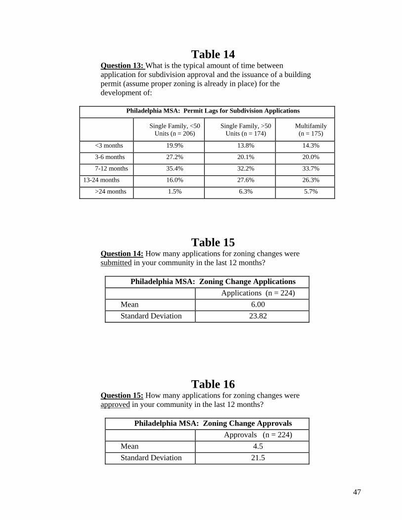
47

Table 14 Question 13: What is the typical amount of time between application for subdivision approval and the issuance of a building permit (assume proper zoning is already in place) for the development of:

Philadelphia MSA: Permit Lags for Subdivision Applications

Single Family, <50 Units (n = 206)

Single Family, >50 Units (n = 174)

Multifamily (n = 175)

<3 months 19.9% 13.8% 14.3%

3-6 months 27.2% 20.1% 20.0%

7-12 months 35.4% 32.2% 33.7%

13-24 months 16.0% 27.6% 26.3%

>24 months 1.5% 6.3% 5.7%

Table 15 Question 14: How many applications for zoning changes were submitted in your community in the last 12 months?

Philadelphia MSA: Zoning Change Applications

Applications (n = 224) Mean 6.00 Standard Deviation 23.82

Table 16 Question 15: How many applications for zoning changes were approved in your community in the last 12 months?

Philadelphia MSA: Zoning Change Approvals

Approvals (n = 224) Mean 4.5 Standard Deviation 21.5

Table 17: Summary Statistics on the WRLURI within the Philadelphia MSA PA Counties NJ Counties

Philadelphia MSA

PA Part

NJ Part Bucks Chester Delaware Mont-

gomery Phila-

delphiaBurling-

ton Camden Gloucester Salem

Mean 1.07 1.11 0.96 1.36 1.59 0.47 0.96 -0.02 1.21 0.68 1.04 0.81 Standard Deviation 0.98 0.95 1.03 1.01 0.79 0.92 0.76 --- 1.00 0.84 1.11 1.36

10th percentile -0.28 -0.23

-0.35

25th percentile 0.31 0.42 0.08 50th percentile 1.13 1.17 0.98 75th percentile 1.64 1.64 1.71 90th percentile 2.35 2.36 2.33

Number of Observations 218 154 64 40 38 31 44 1 20 19 15 9

48

Table 18: Comparing Highly vs. Lightly Regulated Places Philadelphia MSA

WRLURI Range

Regulatory Traits Full Sample

(n=218) WRLURI < 0

(n=38) 0 - 0.5 (n=26)

0.5 - 1.0 (n=31)

1.0 - 2.0 (n=40)

WRLURI > 2.0 (n=33)

Number of Entities That Must Approve Zoning Change Request 1.95 1.61 2.15 2.00 2.03 1.91

Percent With 1 Acre Minimum Lot Size Constraint 58.7 0.0 15.4 51.6 84.4 97.0

Percent With Open Space Requirement 68.3 18.4 46.1 74.2 85.6 90.9

Percent With Exactions Requirements 68.8 26.3 73.1 80.6 78.9 75.8

Average Delay Between Permit Application and Approval - Standardized Projects (# of mo's) 9.2 4.7 5.8 7.4 10.2 16.0

Demographic Traits

Median Family Income (2000) $69,169 $57,323 $61,809 $66,804 $74,688 $75,779

Median House Value (2000) $157,911 $119,032 $138,185 $150,074 $174,041 $181,594

Percent College Graduates (adult population in 2000) 31.0% 24.9% 25.3% 30.1% 34.6% 34.0%

Percent White (2000) 84.9% 77.1% 82.2% 84.4% 86.6% 91.6%

Population (2000) 20,689 52,898 9,644 12,711 15,145 14,913

Land Area (square miles, 2000) 11.9 6.21 7.01 10.9 12.9 20.3

Density (population per square mile, 2000) 2,653 5,387 3,648 2,436 1,960 813

49

50

Table 19: Simple Correlations of WRLURI With Local Traits

WRLURI WRLURI 1.00 Median Family Income 0.37 Median House Value 0.38 Percent College Graduates 0.23

Percent White 0.29 Population -0.07 Land Area 0.37 Density -0.58

Notes: 1. This table is taken from Table 11 of Gyourko, Saiz & Summers. 2. Metropolitan area definitions are based on 1999 boundaries. Consolidated Metropolitan Statistical Areas (CMSAs) are disaggregated into Primary Metropolitan Statistical Areas wherever relevant.

Table 20: Average WRLURI Values--Metropolitan Areas with >10 Observations

Metropolitan Area WRLURI Number of Observations Metropolitan Area WRLURI Number of

Observations1. Providence-Fall River-Warwick, RI-MA 1.76 16 25. Detroit, MI 0.11 46 2. Boston, MA-NH 1.50 41 26. Allentown-Bethlehem-Easton, PA 0.10 14 3. Monmouth-Ocean, NJ 1.17 15 27. Chicago, IL 0.08 95 4. Philadelphia, PA 1.07 218 28. Akron, OH 0.08 11 5. San Francisco, CA 1.01 13 29. Pittsburgh, PA 0.05 44 6. Seattle-Bellevue-Everett, WA 0.96 21 30. Nassau-Suffolk, NY 0.05 13 7. Denver, CO 0.85 13 31. Atlanta, GA 0.05 26 8. Bergen-Passaic, NJ 0.74 21 32. Scranton-Wilkes-Barre-Hazelton, PA 0.04 11 9. Phoenix-Mesa, AZ 0.73 18 33. Salt Lake City-Ogden, UT -0.09 19 10. Fort Lauderdale, FL 0.71 16 34. Grand Rapids-Muskegon-Holland, MI -0.12 16 11. New York, NY 0.68 19 35. Tampa-St. Petersburg-Clearwater, FL -0.17 12 12. Riverside-San Bernardino, CA 0.62 20 36. Cleveland-Lorain-Elyria, OH -0.18 31 13. Newark, NJ 0.58 25 37. San Antonio, TX -0.23 12 14. Harrisburg-Lebanon-Carlisle, PA 0.54 15 38. Port Worth-Arlington, TX -0.24 15 15. Los Angeles-Long Beach, CA 0.54 32 39. Houston, TX -0.26 13 16. Springfield, MA 0.54 13 40. Rochester, NY -0.30 13 17. Oakland, CA 0.52 12 41. Dallas, TX -0.33 31 18. San Diego, CA 0.50 11 42. Oklahoma City, OK -0.40 12 19. Hartford, CO 0.47 28 43. Dayton-Springfield, OH -0.50 17 20. Orange County, CA 0.41 14 44. Cincinnati, OH-KY-IN -0.56 27 21. Washington, DC-MD-VA-WV 0.38 12 45. St. Louis, MO-IL -0.71 27 22. Minneapolis-St. Paul, MN-WI 0.35 48 46. Indianapolis, IN -0.75 12 23. Portland-Vancouver, OR-WA 0.30 20 47. Kansas City, MO-KS -0.79 29 24. Milwaukee-Waukesha, WI 0.29 21

51

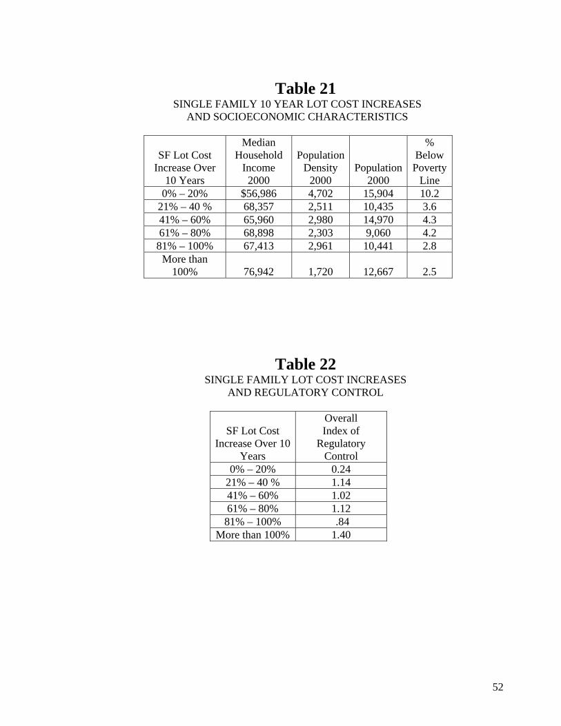
52

Table 21

SINGLE FAMILY 10 YEAR LOT COST INCREASES AND SOCIOECONOMIC CHARACTERISTICS

SF Lot Cost Increase Over

10 Years

Median Household

Income 2000

Population Density

2000 Population

2000

% Below Poverty

Line 0% – 20% $56,986 4,702 15,904 10.2

21% – 40 % 68,357 2,511 10,435 3.6 41% – 60% 65,960 2,980 14,970 4.3 61% – 80% 68,898 2,303 9,060 4.2

81% – 100% 67,413 2,961 10,441 2.8 More than

100% 76,942 1,720 12,667 2.5

Table 22 SINGLE FAMILY LOT COST INCREASES

AND REGULATORY CONTROL

SF Lot Cost Increase Over 10

Years

Overall Index of

Regulatory Control

0% – 20% 0.24 21% – 40 % 1.14 41% – 60% 1.02 61% – 80% 1.12 81% – 100% .84

More than 100% 1.40