report # matc-unl: 427 final...
TRANSCRIPT

®
The contents of this report reflect the views of the authors, who are responsible for the facts and the accuracy of the information presented herein. This document is disseminated under the sponsorship of the Department of Transportation
University Transportation Centers Program, in the interest of information exchange. The U.S. Government assumes no liability for the contents or use thereof.
Impact of Truck Loading on Design and Analysis of Asphaltic Pavement Structures-Phase III
Report # MATC-UNL: 427 Final Report
Yong-Rak Kim, Ph.D. Associate ProfessorDepartment of Civil EngineeringUniversity of Nebraska-Lincoln
2012
A Cooperative Research Project sponsored by the U.S. Department of Transportation Research and Innovative Technology Administration
Hoki Ban, Ph.D.Postdoctoral Research Associate
Soohyok Im Ph.D. Candidate
Impact of Truck Loading on Design and Analysis
of Asphaltic Pavement Structures-Phase III
Yong-Rak Kim, Ph.D.
Associate Professor
Department of Civil Engineering
University of Nebraska-Lincoln
Hoki Ban, Ph.D.
Postdoctoral Research Associate
Department of Civil Engineering
University of Nebraska-Lincoln
Soohyok Im
Ph.D. Candidate
Department of Civil Engineering
University of Nebraska-Lincoln
A Report on Research Sponsored by
Mid-America Transportation Center
University of Nebraska-Lincoln
March 2012

ii
Technical Report Documentation Page
1. Report No.
25-1121-0001-427
2. Government Accession No.
3. Recipient's Catalog No.
4. Title and Subtitle
Impact of Truck Loading on Design and Analysis of Asphaltic Pavement
Structures-Phase III
5. Report Date
March 2012
6. Performing Organization Code
7. Author(s)
Soohyok Im, Hoki Ban, and Yong-Rak Kim 8. Performing Organization Report No.
25-1121-0001-427
9. Performing Organization Name and Address
Mid-America Transportation Center
2200 Vine St.
PO Box 830851
Lincoln, NE 68583-0851
10. Work Unit No. (TRAIS)
11. Contract or Grant No.
12. Sponsoring Agency Name and Address
Research and Innovative Technology Administration
1200 New Jersey Ave., SE Washington, D.C. 20590
13. Type of Report and Period Covered
Final Report
July 2010-March 2012
14. Sponsoring Agency Code
MATC TRB RiP No. 28480
15. Supplementary Notes
16. Abstract
This study investigated the impact of the realistic constitutive material behavior of asphalt layer (both nonlinear inelastic
and fracture) for the prediction of pavement performance. To this end, this study utilized a cohesive zone model to consider
the fracture behavior of asphalt mixtures at an intermediate temperature condition. The semi-circular bend (SCB) fracture
test was conducted to characterize the fracture properties of asphalt mixtures. Fracture properties were then used to
simulate mechanical responses of pavement structures. In addition, Schapery’s nonlinear viscoelastic constitutive model
was implemented into the commercial finite element software ABAQUS via a user defined subroutine (user material, or
UMAT) to analyze asphalt pavement subjected to heavy truck loads. Extensive creep-recovery tests were conducted at
various stress levels and multiple service temperatures to obtain the stress- and temperature-dependent viscoelastic material
properties of asphalt mixtures. Utilizing the derived viscoelastic and fracture properties and the UMAT code, a typical
pavement structure was modeled that simulated the effect of material nonlinearity and damage due to repeated heavy truck
loads. Two-dimensional finite element simulations of the pavement structure demonstrated significant differences between
the cases: linear viscoelastic and nonlinear viscoelastic modeling with and without fracture in the prediction of pavement
performance. The differences between the cases were considered significant, and should be addressed during the process of
performance-based pavement design. This research demonstrates the importance of accurate and more realistic
characterizations of pavement materials.
17. Key Words
Asphalt pavement, performance modeling, nonlinear
viscoelasticity, fracture, finite element method
18. Distribution Statement
19. Security Classif. (of this report)
Unclassified
20. Security Classif. (of this page)
Unclassified
21. No. of Pages
57
22. Price

iii
Table of Contents
Acknowledgments vii
Disclaimer viii
Abstract ix
Chapter 1 Introduction 1
1.1 Research Scope and Objective 3
1.2 Organization of the Report 4
Chapter 2 Literature Review 5
2.1 Studies on Rutting 5
2.2 Studies on Cracking 7
Chapter 3 Nonlinear Viscoelasticity and Cohesive Zone Model 11
3.1 Schapery’s Nonlinear Viscoelastic Model 11
3.2 Cohesive Zone Model 18
Chapter 4 Materials and Laboratory Tests 22
4.1 Materials 22
4.2 Specimen Fabrication 22
4.3 Creep-Recovery Test 27
4.4 SCB Fracture Test 28
Chapter 5 Characterization of Material Properties 31
5.1 Viscoelastic Material Properties 37
5.2 Fracture Properties 37
Chapter 6 Finite Element Analysis of Pavement 41
6.1 Pavement Geometry and Boundary Conditions 41
6.2 Layer Properties 43
6.3 Simulation Results 44
6.3.1 Permanent Deformation (Rut Depth) 45
6.3.2 Horizontal Strain 48
6.3.3 Crack Opening 50
Chapter 7 Summary and Conclusions 52
References 54

iv
List of Figures
Figure 2.1 Test results from Masad and Somadevan (2002) 7
Figure 2.2 Fracture behavior at intermediate service temperatures 9
Figure 3.1 Example problem to verify UMAT code 15
Figure 3.2 Code verification results: Comparisons between analytical and numerical 18
Figure 3.3 Schematic illustration of FPZ of typical quasi-brittle materials 19
Figure 4.1 A specimen cored and sawn from the gyratory compacted sample 23
Figure 4.2 A device used to place the mounting studs for LVDTs 24
Figure 4.3 A specimen with LVDTs mounted in the UTM-25kN 24
Figure 4.4 SCB specimen fabrication and fracture testing configuration 24
Figure 4.5 An overview and a closer view of SCB fracture testing 26
Figure 4.6 Creep-recovery test results at various stress levels 28
Figure 4.7 SCB test results at different loading rates and at 30˚C 29
Figure 5.1 A schematic of a single creep-recovery test 32
Figure 5.2 Comparison plots between model predictions and test results 36
Figure 5.3 A finite element modeling of the SCB testing 38
Figure 5.4 SCB test results vs. cohesive zone model simulation results (force-NMOD) 39
Figure 5.5 SCB Test results vs. cohesive zone model simulation results (force-NTOD) 39
Figure 6.1 A pavement geometry and boundary conditions for finite element modeling 42
Figure 6.2 Truck loading configuration (Class 9) used in this study 43
Figure 6.3 Comparison of permanent deformation up to 50 loading cycles 46
Figure 6.4 Contour plots of vertical displacement distributions 47
Figure 6.5 Comparison of horizontal strain plots 49
Figure 6.6 Depth-tensile stress curve: LVE vs. NLVE 50
Figure 6.7 Depth-crack opening curve: LVE vs. NLVE 51

v
List of Tables
Table 4.1 Mixture information 22
Table 4.2 Applied stress levels for each mixture 27
Table 5.1 Viscoelastic properties determined through the characterization
process 33
Table 5.2 Nonlinear viscoelastic parameters determined 35
Table 5.3 Cohesive zone fracture parameters determined 40
Table 6.1 Material properties of each layer 44

vi
List of Abbreviations
Bituminous Foundation Course (BFC)
Digital Image Correlation (DIC)
Fracture Process Zone (FPZ)
Linear Elastic Fracture Mechanics (LEFM)
Linear Variable Differential Transformers (LVDT)
Mechanistic-Empirical (M-E)
Mechanistic-Empirical Pavement Design Guide (MEPDG)
Notch Mouth Opening Displacements (NMOD)
Notch Tip Opening Displacements (NTOD)
Portland cement concrete (PCC)
Semi-Circular Bend (SCB)
User Material (UMAT)

vii
Acknowledgments
The authors would like to thank the Mid-America Transportation Center (MATC) for
providing the financial support necessary to complete this study.

viii
Disclaimer
The contents of this report reflect the views of the authors, who are responsible for the
facts and the accuracy of the information presented herein. This document is disseminated under
the sponsorship of the Department of Transportation University Transportation Centers Program,
in the interest of information exchange. The U.S. Government assumes no liability for the
contents or use thereof.
ix
Abstract
This study investigated the impact of the realistic constitutive material behavior of
asphalt layer (both nonlinear inelastic and fracture) for the prediction of pavement performance.
To this end, this study utilized a cohesive zone model to consider the fracture behavior of asphalt
mixtures at an intermediate temperature condition. The semi-circular bend (SCB) fracture test
was conducted to characterize the fracture properties of asphalt mixtures. Fracture properties
were then used to simulate mechanical responses of pavement structures. In addition, Schapery’s
nonlinear viscoelastic constitutive model was implemented into the commercial finite element
software ABAQUS via a user defined subroutine (user material, or UMAT) to analyze asphalt
pavement subjected to heavy truck loads. Extensive creep-recovery tests were conducted at
various stress levels and multiple service temperatures to obtain the stress- and temperature-
dependent viscoelastic material properties of asphalt mixtures. Utilizing the derived viscoelastic
and fracture properties and the UMAT code, a typical pavement structure was modeled that
simulated the effect of material nonlinearity and damage due to repeated heavy truck loads. Two-
dimensional finite element simulations of the pavement structure demonstrated significant
differences between the cases: linear viscoelastic and nonlinear viscoelastic modeling with and
without fracture in the prediction of pavement performance. The differences between the cases
were considered significant, and should be addressed during the process of performance-based
pavement design. This research demonstrates the importance of accurate and more realistic
characterizations of pavement materials.
1
Chapter 1 Introduction
Distresses in asphalt pavements, such as rutting and fatigue cracking, are critical safety
issues affecting roadway users. Rutting, or, permanent deformation, is surface depression
resulting from the accumulation of vertical displacements in asphalt pavement layers. The
presence of this distress is even more dangerous for roadway users when the surface depression
is filled with water. Accumulation of water in surface depressions increases the risk of vehicle
hydroplaning, and, as a result of freezing and thawing cycles in cold regions, weakens pavement
layers. Large damage areas, such as potholes, result from severe fatigue cracking in the
pavement, combined with thermal stress. Pavement design methods should account for the
combination of multiple factors that cause these distresses (i.e., traffic loads, environmental
effects, and composite material constituent’s combinations and interactions), in order to improve
the reliability of the structures.
A few approaches have been adopted by the research community to examine the effects
of these distress-causing factors on pavement response. Conventional asphalt pavement design
methods assume that asphalt layers are made of materials with linear-elastic response; however,
asphaltic materials exhibit viscoelastic material behavior that is significantly affected by the rate
of loading, time, and temperature conditions. It has been observed that results from elastic
analyses do not correlate well with field measurements. To improve the accuracy of these
analyses, many studies have adopted the viscoelastic constitutive model to predict the behavior
of asphaltic materials (Al-Qadi et al. 2005; Elseifi et al. 2006; Yoo 2007; Kim et al. 2008; Kim et
al. 2009). However, nonlinear response was not taken into consideration in these models in spite
of abundant experimental observations (Masad and Somadevan 2002; Collop et al. 2003; Airey et
al. 2004) that present nonlinear response of asphalt binders and mixes at certain levels of stress

2
and strain. Therefore, it is necessary to consider stress-dependent nonlinear viscoelastic material
characteristics at various stress levels.
To this end, this study characterized the nonlinear viscoelastic behavior of asphalt
mixtures using Schapery’s nonlinear viscoelastic model. The model was implemented into the
commercial finite element software ABAQUS as a user-defined subroutine, labeled UMAT (user
material) based on the recursive-iterative numerical algorithm determined by Haji-Ali and
Muliana (2004). Extensive creep-recovery tests were conducted at various stress levels and at
two temperatures (30oC and 40
oC) in order to obtain the stress- and temperature-dependent
nonlinear viscoelastic material properties of asphalt mixtures. Material properties were then used
to simulate mechanical responses of pavement structures. Detailed investigations of the
pavement responses resulting from different constitutive relations (such as linear viscoelastic and
nonlinear viscoelastic) can provide better understanding of the effects of truck loading on
pavement damage and consequently advance the current pavement analysis-design method.
The recent mechanistic-empirical (M-E) design guide predicts fatigue cracking resistance
of asphalt pavements by considering various factors mentioned above. However, the M-E design
guide is known to be limited in its ability to accurately predict mechanical responses in asphaltic
pavements due to the use of empirically developed prediction models. Recently, the fracture
behavior of asphalt mixtures has been studied by several researchers through fracture tests and
numerical analysis by means of a cohesive zone model (Marasteanu et al. 2002; Wagoner et al.
2005, 2006; Kim et al. 2008). Most studies were conducted at low temperature conditions;
however, since fracture behavior at intermediate service temperatures is sensitive to loading
rates, this study considered the fracture behavior of asphalt mixtures at an intermediate
temperature condition (30oC) using the cohesive zone model. The SCB fracture test was

3
conducted to characterize the fracture properties of asphalt mixtures. Fracture properties were
then used to simulate mechanical responses of pavement structures subjected to heavy truck
loads.
1.1 Research Scope and Objective
The purpose of the current study was to provide a better understanding of the effects of
heavy-load trucks on pavement performance. Trucking is the most dominant component of U.S.
freight transportation, and is expected to grow significantly in the future. Better preservation of
the existing highway infrastructure against heavy-load trucks is therefore a necessity. Success in
this endeavor can be achieved through more accurate and realistic analyses of pavement
structures.
For a more accurate and realistic analysis of pavement structures against heavy-load
trucks, a series of research efforts led by the primary investigator was initiated in FY 2009 and
continued in FY 2010. These efforts investigated pavement performance predictions from both
the newly released “Mechanistic-Empirical Pavement Design Guide” (MEPDG) approach and
the purely mechanistic approach based on the “Finite Element Method.” The research
particularly focused on the impact of heavy truck loads on pavement damage. Analysis results
during FY 2009 and FY 2010 clearly demonstrated that both material inelasticity (e.g., the
viscoelastic nature of asphaltic materials and elasto-plastic behavior of soils) and realistic tire
loading configuration, which are not rigorously implemented in the current MEPDG, can mislead
predictions of pavement rutting. These misled predictions can result in significant errors in the
design of pavement structure as well as in the prediction of pavement performance when the
empirical damage evolution relations in the MEPDG are further incorporated.

4
Based on research outcomes observed during FY 2009 and FY 2010, this study, “Phase
III” extends the previous research scope to facilitate a more realistic analysis of pavement
performance. In this study, a more detailed investigation of pavement responses was pursued by
focusing on the fracture- (cracking) related damage behavior of pavement structures. Any
significant differences between the cases were considered important factors that should be
deliberately examined for a more precise implementation of pavement analysis and design in
future research.
1.2 Organization of the Report
This report is composed of seven chapters. Following the current introduction, chapter 2
summarizes literature on rutting and cracking. Chapter 3 presents the theoretical background of
Schapery’s nonlinear viscoelastic constitutive model and its numerical implementation into a
finite element code. The theoretical background of the cohesive zone model is also presented in
chapter 3. Chapter 4 describes the creep-recovery test and the fracture test conducted to identify
viscoelastic and fracture properties of asphalt mixtures. Chapter 5 describes how the viscoelastic
and fracture properties were obtained from the laboratory test results. From the material
properties identified in chapter 5, chapter 6 describes finite element simulations of a pavement
structure, taking into account the effect of material viscoelasticity (linear and nonlinear) and
fracture of pavement subjected to heavy truck loads. Simulation results and significant
observations are discussed. Finally, chapter 7 summarizes this study and its conclusions.
5
Chapter 2 Literature Review
2.1 Studies on Rutting
Rutting is one of the primary distresses in flexible pavement systems. Rutting is caused
by plastic or permanent deformation in the asphalt concrete, unbound layers, and foundation
soils. The M-E design guide predicts rutting performance of flexible pavements by considering
the constitutive relationship between predicted rutting in the asphalt mixture and field-calibrated
statistical analyses of repeated load permanent deformation tests conducted in the laboratory.
The laboratory-derived relationship is then adjusted to match the rut depth measured from the
roadway (AASHTO 2008).
Although the M-E design guide employs various design parameters (climate, traffic,
materials, etc.) to predict the performance of flexible pavements, it is known to be limited in its
ability to accurately predict mechanical responses in asphaltic pavements due to the use of
simplified structural analysis methods, a general lack of understanding of the fundamental
constitutive behavior and damage mechanisms of paving materials, and the use of circular tire
loading configurations.
To overcome the limitations of the layered elastic approaches, many researchers have
attempted to develop structural mechanistic models that are able to predict the performance of
asphaltic pavements. In order to represent the behavior of asphalt mixtures under different
boundary conditions, it is necessary to incorporate constitutive material models into these
structural mechanistic models. Computational approaches such as the finite element technique
have received increased attention from the pavement mechanics community due to their
extremely versatile implementation of mechanical characteristics in addressing complex issues
such as inelastic constitutive behavior, irregular pavement geometry (Blab and Harvey 2002; Al-

6
Qadi et al. 2002; Collop et al. 2003; Al-Qadi et al. 2004; Al-Qadi et al. 2005), and growing
damage (Mun et al. 2004; Elseifi and Al-Qadi 2006; Kim et al. 2006).
Recently, several studies (Al-Qadi et al. 2005; Elseifi et al. 2006; Kim et al., 2009) have
conducted viscoelastic analyses that considered the asphalt layer as linear viscoelastic and the
other layers as elastic, using the finite element method in two dimensional (2-D) or three-
dimensional (3-D) models for predicting the time-dependent response of flexible pavement.
However, nonlinear response was not taken into consideration in these models, in spite of
abundant experimental observations (Masad and Somadevan 2002; Collop et al. 2003; Airey et
al. 2004) that demonstrated nonlinear response of asphalt binders and mixes at certain levels of
stress and strain. For example, figure 2.1, which presents test results from Masad and Somadevan
(2002), illustrates that the nonlinearity is evident as the shear modulus decreases with an increase
in strain level. For a linear material, the curves in the figure would coincide. Therefore, it is
necessary to consider the nonlinear viscoelastic responses when asphalt pavements are subjected
to heavy loads.

7
Figure 2.1 Test results from Masad and Somadevan (2002)
2.2 Studies on Cracking
Various asphalt pavement distresses are related to fracture including fatigue cracking
(both top-down and bottom-up), thermal (transverse) cracking, and reflective cracking of the
asphalt layer. Cracking in asphaltic pavement layers causes primary failure of the roadway
structure and leads to long-term durability issues, and are often related to moisture damage. The
fracture resistance and characteristics of asphalt materials significantly influence the service life
of asphalt pavements and consequently the maintenance and management of the pavement
network. In spite of its significant implications, proper characterization of the fracture process
and fundamental fracture properties of the asphaltic materials have not been adopted in the
current pavement design-analysis procedures which are generally phenomenological.
Cracking is probably the most challenging issue to predict and control. This is because of
the complex geometric characteristics and inelastic mechanical behavior of the asphalt mixtures,

8
which are temperature sensitive and rate dependent. These characteristics make any solution to
the cracking problem in asphalt mixtures almost impossible to achieve via the theory of linear
elastic fracture mechanics (LEFM). LEFM is only able to predict the stress state close to the
crack tips of damaged bodies if the fracture process zone (FPZ) around the crack tip is very
small. The FPZ in asphaltic materials might be large, as is typical of quasi-brittle materials
(Bazant and Planas 1998).
Some studies have evaluated the fracture toughness of asphalt mixtures using the J-
integral concept or the stress intensity approach (Mobasher et al. 1997; Mull et al. 2002; Kim et
al., 2003). Others have conducted fracture tests and numerical analyses by means of a cohesive
zone model to study the fracture behavior of asphalt mixtures (Li and Marasteanu 2005; Song et
al. 2006; Kim et al. 2007; Kim et al. 2009). The cohesive zone modeling approach has recently
received increased attention from the asphaltic materials and pavement mechanics community
for modeling crack initiation and growth. The cohesive zone approach can properly model both
brittle and ductile fracture, which is frequently observed in asphaltic roadways due to the wide
range of service temperatures and traffic speeds. Moreover, it can provide an efficient tool that
can be easily implemented in various computational methods, such as finite element and discrete
element methods, so that fracture events in extremely complicated mixture microstructure can
also be simulated.
To monitor averaged deformations or displacements for the characterization of fracture
properties of asphalt mixtures, most fracture tests have traditionally used conventional
extensometers or clip-on gauges far from the actual FPZ. However, the true fracture properties of
asphalt mixtures could be misled by as much as an order of magnitude, since the material
responses captured by the extensometers or clip-on gauges are limited in their ability to

9
accurately represent material behavior at the actual FPZ. This discrepancy can worsen if the
material is highly heterogeneous and inelastic (Song et al. 2008; Aragão 2011), which is typical
in asphaltic paving materials. In addition, most of the studies have adopted low-temperature
testing conditions in which the type of fracture is much more brittle and elastic. However, as
shown in figure 2.2 (Aragão and Kim 2011), fracture behavior of asphaltic materials at
intermediate service temperatures is sensitive to the loading rates. In order to accurately
characterize intermediate temperature fracture behavior such as fatigue cracking, Aragão and
Kim (2011) conducted fracture tests at 21o C. Test results presented significant rate-dependent
behavior.
Figure 2.2 Fracture behavior at intermediate service temperatures
A better understanding of the FPZ at realistic service conditions is a critical step in the
development of mechanistic design-analysis procedures for asphaltic mixtures and pavement

10
structures. This is because characteristics of the FPZ represent the true material behavior relative
to fracture damage, which, consequently, leads to the selection of proper testing methods and
modeling-analysis techniques that appropriately address the complex local fracture process.
However, such careful efforts to characterize the FPZ in asphalt concrete mixtures have been, to
date, insufficient. To our best knowledge, only limited attempts (Kim et al. 2002; Seo et al. 2002;
Song et al. 2008; Li and Marasteanu 2010) have been carried out due to the many experimental-
analytical complexities.

11
Chapter 3 Nonlinear Viscoelasticity and Cohesive Zone Model
The current chapter presents more advanced constitutive models for better
characterization and performance prediction of asphalt mixtures. A multiaxial nonlinear
viscoelastic constitutive model developed by Schapery (1969) is briefly introduced, and the
numerical implementation incorporated with the finite element method is described. Schapery’s
single integral constitutive model was implemented into the commercial finite element software
ABAQUS via a user-defined material called UMAT. In accordance with Schapery’s model, the
cohesive zone model was described to account for the fracture process as a gradual separation.
3.1 Schapery’s Nonlinear Viscoelastic Model
Schapery’s nonlinear viscoelastic single-integral constitutive model (Schapery 1969) for
one-dimensional problems can be expressed in terms of an applied stress () as follows:
2
0 0 1
0
( ) ( )
td g
t g D g D t dd
(3.1)
where,
is the reduced time given by:
0
td
ta
(3.2)
where,
g0, g1, g2 and aσ are the nonlinear viscoelastic parameters associated with stress level.
These parameters are always positive and equal to 1 for the Boltzmann integral in linear
viscoelasticity. It is noted that equation 3.2 can include not only stress effect, but also effects

12
such as temperature, moisture, and physical aging as each shift factor. D0 and ΔD are uniaxial
instantaneous and transient creep compliance at linear viscoelasticity respectively. The uniaxial
transient compliance can be expressed in the form of a Prony series as:
1
1 exp
N
n n
n
D D
(3.3)
where,
N is the number of Prony series, and Dn and λn are nth coefficient of the Prony series and
the nth reciprocal of retardation time, respectively. Therefore equation 3.1 can be rewritten by
substituting equation 3.3 into equation 3.1 as:
0 0 1 2 1
1 1
N N
n n n
n n
t g D g g D g D Q
(3.4)
where,
2
0
exp
t
n n
dgQ t d
d
(3.5)
The one-dimensional integral in equation 3.1 can be generalized to describe the multi-
axial (i.e., 3-D) constitutive relations for an isotropic media by decoupling the response into
deviatoric and volumetric strains as follows (Lai and Bakker 1996):

13
2
0 0 1
0
1 1
2 2
t
ij
ij ij
d g Se t g J S g J t d
d
(3.6)
2
0 0 1
0
1 1
3 3
t
kk
kk kk
d gt g B g B t d
d
(3.7)
where,
eij, εkk , and Sij are deviatoric strain, volumetric strain, and deviatoric stress, respectively.
J0, B0, ΔJ, and ΔB are the instantaneous and transient elastic shear and bulk compliance,
respectively. The shear transient compliance ΔJ(ψ) and the bulk transient compliance ΔB(ψ) can
also be expressed by the Prony series as follows:
1
1 exp
N
n n
n
J J
(3.8)
1
1 exp
N
n n
n
B B
(3.9)
Assuming that Poisson’s ratio υ is time-independent, the instantaneous and transient
shear and bulk compliance can be evaluated from the following relations:
0 0 0 02 1 3 1 2
2 1 3 1 2
J D B D
J D B D
(3.10)
The nonlinear parameters are assumed to be general polynomial functions of the effective
shear stress which can be written as (Haji-Ali and Muliana 2004):

14
0 1
0 01 1
2
0 01 1
1 1 , 1 1
1 1 , 1 1
n ni i
i i
i i
n ni i
i i
i i
g g
g a
(3.11)
where,
, 0 3,
0, 0 2ij ij
x xx S S
x
The polynomial coefficients (i, i, i, i) can be calibrated from the creep and recovery
tests at various stress levels. The term 0 is the effective shear stress limit in the linear
viscoelastic range.
Next, the deviatoric and volumetric components can be expressed in terms of the
hereditary integral formulation by substituting equation 3.8 into equation 3.6 and equation 3.9
into equation 3.7 as follows (Haji-Ali and Muliana 2004):
0 0 1 2 ,
1 1
1
2
N N
ij n ij ij n
n n
e t g J g g J S Q
(3.12)
0 0 1 2 ,
1 1
1
3
N N
kk n kk kk n
n n
t g B g g B Q
(3.13)

15
where,
2
, 1
0
1exp
2
t
ij
ij n n n
d g SQ g J t d
d
(3.14)
2
, 1
0
1exp
3
t
kk
kk n n n
d gQ g B t d
d
(3.15)
The derived 3-D nonlinear viscoelastic equations were numerically implemented into the
well-known commercial finite element software ABAQUS via a user-defined material called
UMAT, using the recursive integration scheme developed by Haj-Ali and Muliana (2004). In an
attempt to verify whether the UMAT subroutine code was properly implemented in the finite
element mainframe, one simple example problem was introduced. Code verification can be
conducted simply by comparing computational results from the finite element code to analytical
results obtained from the easily solvable problem. The example problem to be analyzed for code
verification is shown in figure 3.1.
1 m
1 m
a a b at H t H t t
Stre
ss
a
b
at bt (sec)t
Figure 3.1 Example problem to verify UMAT code

16
Supposing a simple viscoelastic uniaxial bar is subjected to a two-step tensile load as
presented in figure 3.1, the first loading of 1.0N is applied for 10 seconds, then reduced to 0.5N
for 40 seconds. The resulting strain response can be derived as:
0 0 1 2
a a a
c aa
tt g D g g D
a
for 0 at t (3.16)
0 0 1 2 2 2
b b a b aa a ar b a b aa b b
t t t t tt g D g g D g g D
a a a
for a bt t t
(3.17)
The creep compliance D t is linear viscoelastic material property represented as the
Prony series. Since this problem is merely for the sake of code verification, a simple form of the
creep compliance is assumed as follows:
0 1 1 expD t D D t (3.18)
where,
0
0
1D
E , 0 1E E E , 1
0
1 1D
E E
, 0
1E
E

17
For the UMAT code verification, a special case of nonlinear viscoelastic response where
0 1 2 1g g g a was first simulated. When the nonlinear viscoelastic model parameters are
all equal to unity, the nonlinear viscoelastic model reduces to a linear viscoelastic hereditary
integral. An analytical linear viscoelastic solution can then be calculated and compared to the
computational results from the finite element analysis. Good agreement between the two results
infers that the code was developed appropriately. As shown in figure 3.2, the linear viscoelastic
finite element prediction and analytical solution match very well.
Secondly, in an attempt to examine the role of material nonlinearity in the model, the
same uniaxial bar problem was simulated by assigning that the two parameters ( 0
ag and aa ) are
equal to unity, while the other two nonlinear parameters are assumed as 21 1.1a ag g during the
first loading stage and returned to unity when the second loading is applied. Tensile strains when
the uniaxial bar is nonlinear viscoelastic are also plotted in figure 3.2. As shown, the finite
element prediction and analytical solution are identical. Another observation to be noted from the
figure is that instantaneous strains resulting from all four cases are identical, but later stage
strains from the nonlinear viscoelastic cases are greater than those from the linear viscoelastic
cases. This seems reasonable because the nonlinear parameter 0
ag , which contributes to
instantaneous response, was set equal to unity, and the other two parameters that affect later
stage responses represented nonlinear viscoelastic behavior. This confirms that the UMAT code
equipped with the nonlinear viscoelastic feature was developed appropriately and can be used to
simulate nonlinear viscoelastic responses of general structures (such as pavements) that are
typically associated with complicated geometry and boundary conditions.

18
Time (sec)
0 10 20 30 40 50
Str
ain
0.0
2.0e-6
4.0e-6
6.0e-6
8.0e-6
1.0e-5
1.2e-5
Analytical (linear)
Analytical (nonlinear)
Numerical (linear)
Numerical (nonlinear)
Figure 3.2 Code verification results: Comparisons between analytical and numerical
3.2 Cohesive Zone Model
The FPZ is a nonlinear zone characterized by progressive softening, for which the stress
decreases at increasing deformation. The nonlinear softening zone is surrounded by a non-
softening nonlinear zone, which represents material inelasticity. Bazant and Planas (1998)
classified the fracture process behavior in certain materials into three types: brittle, ductile, and
quasi-brittle. Each type presents different relative sizes of these two nonlinear zones (i.e.,
softening and non-softening nonlinear zones). Figure 3.3 presents the third type of behavior, so-
called quasi-brittle fracture. It includes situations in which a major part of the nonlinear zone
undergoes progressive damage with material softening due to microcracking, void formation,
interface breakages, frictional slips, and others. The softening zone is then surrounded by the
inelastic material yielding zone, which is much smaller than the softening zone. This behavior

19
includes a relatively large FPZ, as illustrated in figure 3.3. Asphaltic paving mixtures are usually
classified as quasi-brittle materials (Bazant and Planas 1998; Duan et al. 2006; Kim et al. 2008).
softening
nonlinear hardening
T
tip of FPZtip of physical crack
Tmax
FPZ
c
1.0
T/Tmax
/ c1.0
Area = Gc
Bilinear Cohesive Zone Model
Figure 3.3 Schematic illustration of FPZ of typical quasi-brittle materials
The FPZ can be modeled in many different ways. One well-known approach is to use a
cohesive zone. At the crack tip, the cohesive zone constitutive behavior reflects the change in the
cohesive zone material properties due to microscopic damage accumulation ahead of the crack
tip. This behavior can be expressed by the general traction-displacement cohesive zone
relationship as follows:

20
),(),( miimi xTtxT (3.19)
where,
Ti = cohesive zone traction (Tn for normal and Tt for tangential traction),
i cohesive zone displacement (n for normal and t for tangential
displacement),
xm = spatial coordinates, and
t = time of interest.
Cohesive zone models regard fracture as a gradual phenomenon in which separation ()
takes place across an extended crack tip (or cohesive zone) and where fracture is resisted by
cohesive tractions (T). The cohesive zone effectively describes the material resistance when
material elements are being displaced. Equations relating normal and tangential displacement
jumps across the cohesive surfaces with the proper tractions define a cohesive zone model.
Among numerous cohesive zone models developed for various specific purposes, this study used
an intrinsic bilinear cohesive zone model (Geubelle and Baylor 1998; Espinosa and Zavattieri
2003; Song et al. 2006). As shown in figure 3.3, the model assumes that there is a recoverable
linear elastic behavior until the traction (T) reaches a peak value, or cohesive strength (Tmax) at a
corresponding separation in the traction-separation curve. At that point, a non-dimensional
displacement () can be identified and used to adjust the initial slope in the recoverable linear
elastic part of the cohesive law. This capability of the bilinear model to adjust the initial slope is
significant, because it can alleviate the artificial compliance inherent to intrinsic cohesive zone
models. The value was determined through a convergence study designed to find a value
sufficiently small enough to guarantee a level of initial stiffness that renders artificial compliance

21
of the cohesive zone model insignificant. It was observed that a numerical convergence can be
met when the effective displacement is smaller than 0.0005, which was used for simulations in
this study. Upon damage initiation, T varies from Tmax to 0, when a critical displacement (c) is
reached and the faces of the cohesive element are fully and irreversibly separated. The cohesive
zone fracture energy (Gc), which is the locally estimated fracture toughness, can then be
calculated by computing the area below the bilinear traction-separation curve with peak traction
(Tmax) and critical displacement (c) as follows:
max
2
1Tcc G (3.20)

22
Chapter 4 Materials and Laboratory Tests
This chapter briefly describes the materials used and the laboratory tests performed in
this study. An asphalt mixture was selected for creep-recovery tests at varying stress levels in
order to determine its linear and nonlinear viscoelastic material characteristics. The SCB fracture
test was conducted at the same testing temperature (30 o
C) to identify fracture properties of the
mixture.
4.1 Materials
Table 4.1 summarizes mixture information, including Superpave PG asphalt binder grade,
aggregate gradation of the mixture, and resulting binder content to satisfy mixture volumetric
requirements. Binder content of 6.00% was determined as an appropriate value that satisfied all
key volumetric characteristics of the asphalt mixture including the 4% ± 1% air voids.
Table 4.1 Mixture information
Mixture
ID
Binder
PG
Aggregate Gradation (% Passing on Each Sieve) %
Binder
%
Voids 19mm 12.5mm 9.5mm #4 #8 #16 #30 #50 #200
AC
Mixture 64-28 100 95 89 72 36 21 14 10 3.5 6.00 4.09
4.2 Specimen Fabrication
To conduct the uniaxial static creep-recovery tests, a Superpave gyratory compactor was
used to generate the cylindrical samples with a diameter of 150 mm and an approximate height
of 170 mm. The compacted samples were then cored and sawed to produce testing specimens
targeting an air void of 4% ± 0.5% with a diameter of 100 mm and a height of 150 mm. Figure
4.1 presents a specimen after the compaction and coring-sawing process.

23
Figure 4.1 A specimen cored and sawn from the gyratory compacted sample
To measure the axial displacement of the specimen under the static compressive force,
epoxy glue was used to fix mounting studs to the surface of the specimen so that the three linear
variable differential transformers (LVDTs) could be attached to the surface of the specimen at
120o radial intervals with a 100 mm gauge length, as illustrated in figure 4.2. Next, the specimen
was mounted in the UTM-25kN testing station for creep-recovery testing (fig. 4.3).
Figure 4.4 demonstrates the specimen production process for the SCB fracture test using
the Superpave gyratory compactor and saw machines. The Superpave gyratory compactor was
used to produce tall compacted samples: 150 mm in diameter and 175 mm in height. Five slices
(each with a diameter of 150 mm and a height of 25 mm) were obtained by removing the top and
bottom parts of the tall sample. Finally, the slice was cut into two identical halves, and the saw
machine was used to make a vertical notch 25 mm long and 2.5 mm wide.

24
Figure 4.2 A device used to place the mounting studs for LVDTs
Figure 4.3 A specimen with LVDTs mounted in the UTM-25kN
Figure 4.4 SCB specimen fabrication and fracture testing configuration
In this study, the digital image correlation (DIC) system was incorporated with the SCB
fracture test to characterize fracture properties of the asphalt mixture. The DIC recognizes the

25
surface structure of the specimen in digital video images and allocates coordinates to the image
pixels. The first image represents the undeformed state, and further images are recorded during
the deformation of the specimen. Then, the DIC compares the digital images and calculates the
displacement and deformation of the specimen. In order to facilitate the DIC process more
efficiently, the specimen was painted with black and white spray until a clear contrast between
the white background and numerous black dots (creating an image pattern) was achieved. A
number of black dots were used as material points for the full-field deformation characteristics
such as formation and movement of the FPZ, as cracks grew due to loading. Additionally, two
pairs of dot gauges were attached to the surface of the specimen to more accurately capture the
displacements at the mouth (denoted as notch mouth opening displacements [NMOD]) and at the
tip (denoted as notch tip opening displacements, [NTOD]) of the initial notch. The DIC system
used in this study incorporated a high-speed video camera that can accurately monitor specimen
deformation in strains from 0.05% up to 500%. Figure 4.5 shows the SCB testing set-up, painted
black dot image pattern, and the additional two-pair gauge points attached on the specimen
surface for DIC analysis.

26
(a) an overview of the whole testing set-up
75 mm
150 mm
Clip-on gauge
Black dot image pattern
NTOD dot gauges
NMOD dot gauges
DIC at crack propagation
NTOD
NMOD
(b) a closer view of a SCB specimen ready to be tested
Figure 4.5 An overview and a closer view of SCB fracture testing
calibration panel
SCB specimen
DIC cameras
DIC light source

27
4.3 Creep-Recovery Test
The static creep-recovery test was conducted on replicate specimens of the asphalt
mixture at 30oC. A creep stress for 30 seconds (followed by recovery for 1,000 seconds) was
applied to the specimens, and the vertical deformation (in compression) was monitored with the
three LVDTs. Various stress levels were applied to characterize nonlinear behavior of asphalt
mixtures for a large range of stress levels.
Table 4.2 presents applied stress levels and the testing temperature. Based on the
preliminary test results, the threshold stress (reference stress) of nonlinear viscoelasticity was
found to be 700 kPa. In other words, the asphalt mixture is considered linear viscoelastic below
the reference stress level at that testing temperature. Figure 4.6 presents the test results. As
expected, the higher stress level generated larger creep strain and recovered less strain.
Table 4.2 Applied stress levels for each mixture
Mixture ID Temp. Stress Level (kPa)
AC Mixture 30°C 700 1,000 1,200 1,500

28
Time (sec)
0 100 200 300
Str
ain
0.000
0.002
0.004
0.006
0.008
0.010
0.012
0.014
700 kPa
1000 kPa
1200 kPa
1500 kPa
Figure 4.6 Creep-recovery test results at various stress levels
4.4 SCB Fracture Test
A total of 12 SCB specimens of the asphalt mixture were prepared to complete three
replicates per test case. Prior to testing, individual SCB specimens were placed inside the
environmental chamber of a mechanical testing machine for temperature equilibrium targeting
the testing temperature of 30˚C. Following the temperature conditioning step, specimens were
subjected to a simple three-point bending configuration with four different monotonic
displacement rates (i.e., 1, 5, 10, and 50 mm/min.) applied to the top center line of the SCB
specimens. As shown in figure 4.5, metallic rollers separated by a distance of 122 mm (14 mm
from the edges of the specimen) were used to support the specimen. Reaction force at the loading
point was monitored by the data acquisition system installed in the mechanical testing machine.
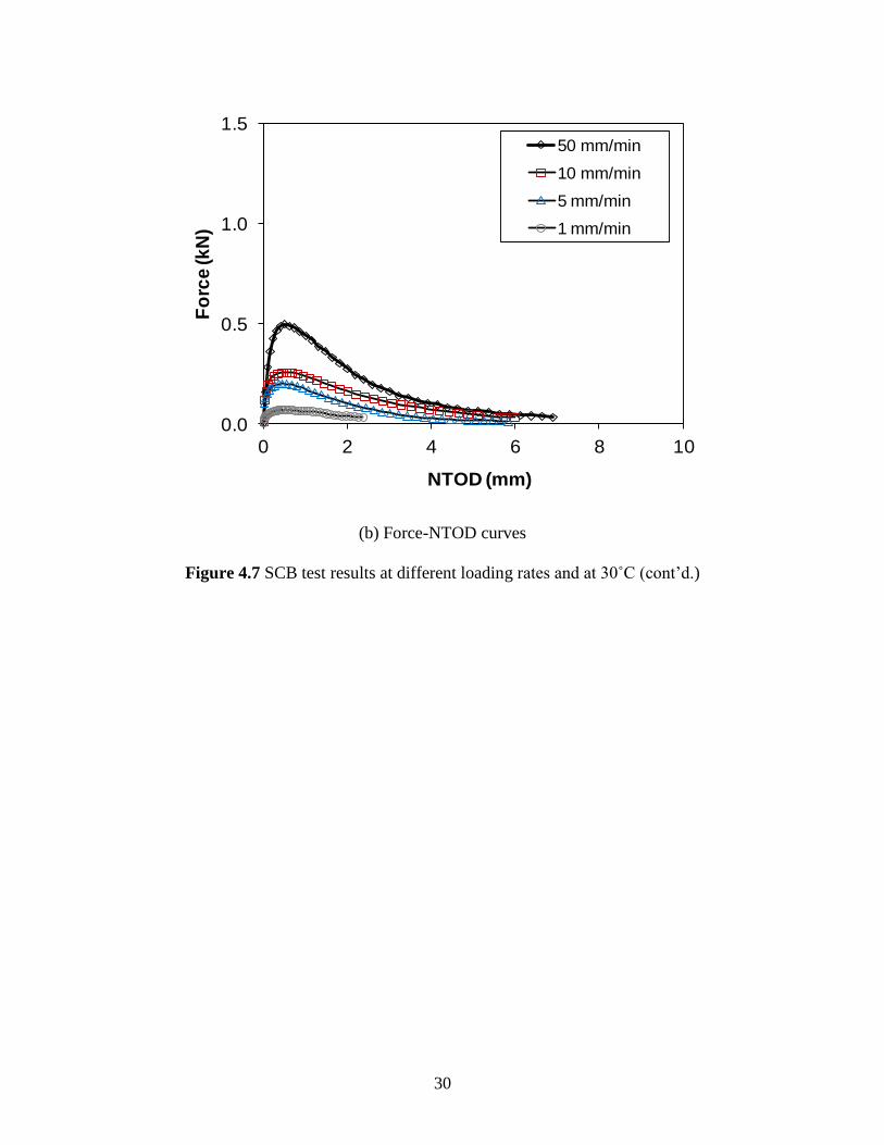
Figure 4.7 presents the SCB test results by plotting the average values between the
reaction forces and opening displacements (NMOD and NTOD) monitored by the DIC system at
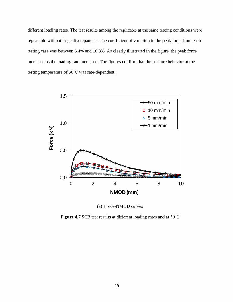
29
different loading rates. The test results among the replicates at the same testing conditions were
repeatable without large discrepancies. The coefficient of variation in the peak force from each
testing case was between 5.4% and 10.8%. As clearly illustrated in the figure, the peak force
increased as the loading rate increased. The figures confirm that the fracture behavior at the
testing temperature of 30˚C was rate-dependent.
0.0
0.5
1.0
1.5
0 2 4 6 8 10
Fo
rce
(k
N)
NMOD (mm)
50 mm/min
10 mm/min
5 mm/min
1 mm/min
(a) Force-NMOD curves
Figure 4.7 SCB test results at different loading rates and at 30˚C
30
0.0
0.5
1.0
1.5
0 2 4 6 8 10
Fo
rce
(kN
)
NTOD (mm)
50 mm/min
10 mm/min
5 mm/min
1 mm/min
(b) Force-NTOD curves
Figure 4.7 SCB test results at different loading rates and at 30˚C (cont’d.)
31
Chapter 5 Characterization of Material Properties
In this chapter, the creep-recovery test and SCB fracture test results presented in the
previous chapter are used to characterize material properties. Using creep-recovery test results,
the linear viscoelastic properties at the threshold stress level are identified, as are the nonlinear
viscoelastic properties at higher stress levels. The viscoelastic material properties are then
validated by comparing test results with numerical simulations of the creep-recovery test.
Regarding the SCB fracture, test results are used to determine fracture properties of the mixture.
The cohesive zone fracture properties in the bilinear cohesive zone model are determined for
each case through the calibration process until a good agreement between test results and finite
element simulations is observed.
5.1 Viscoelastic Material Properties
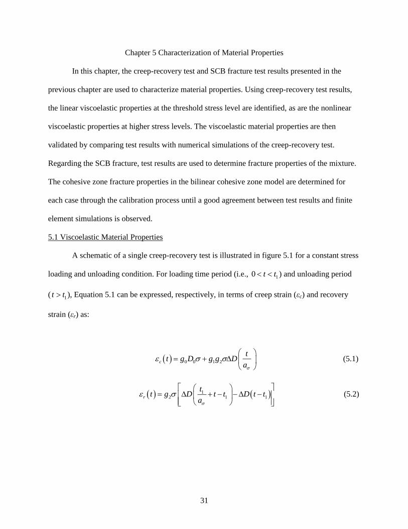
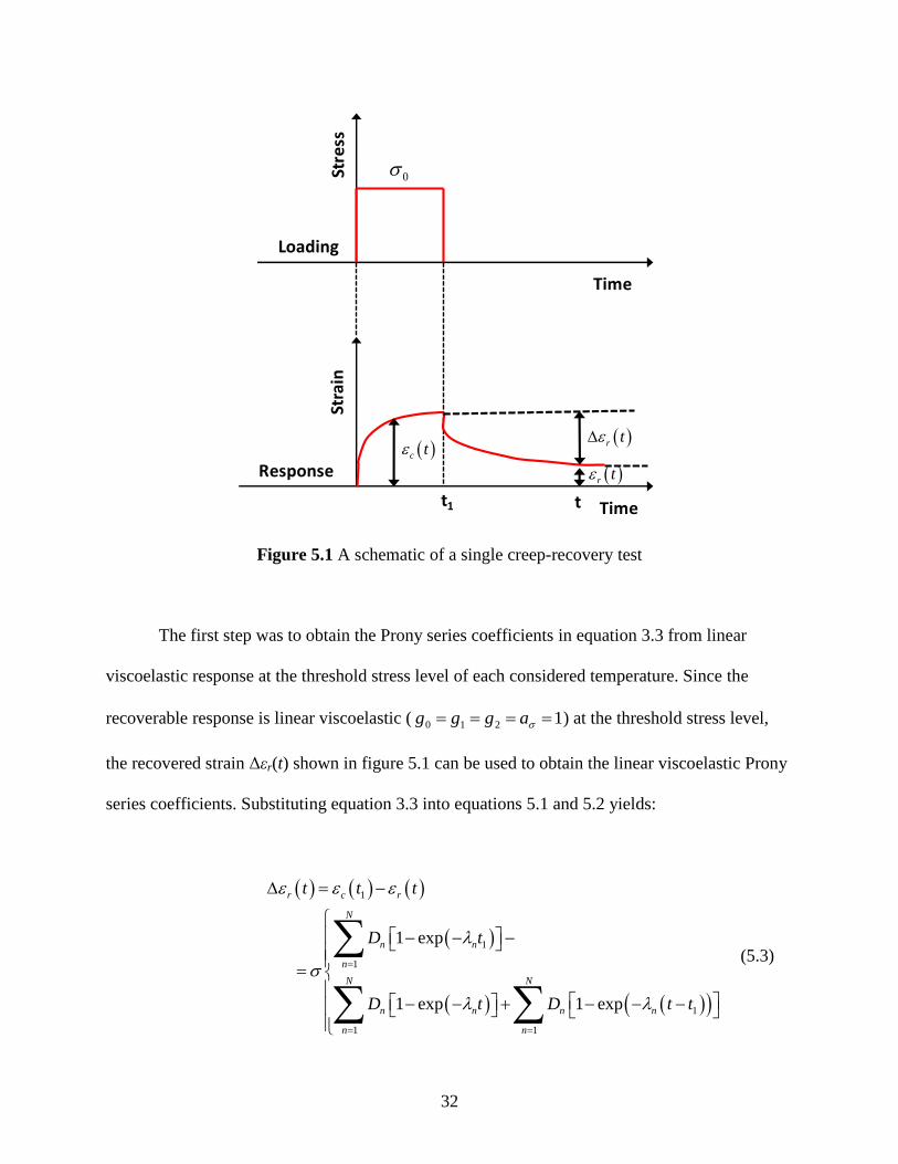
A schematic of a single creep-recovery test is illustrated in figure 5.1 for a constant stress
loading and unloading condition. For loading time period (i.e., 10 tt ) and unloading period
( 1tt ), Equation 5.1 can be expressed, respectively, in terms of creep strain (εc) and recovery
strain (εr) as:
0 0 1 2c
tt g D g g D
a
(5.1)
12 1 1r
tt g D t t D t t
a
(5.2)
32
Stre
ssSt
rain
Loading
Response
0
c t r t
r t
Time
Timet1 t
Figure 5.1 A schematic of a single creep-recovery test
The first step was to obtain the Prony series coefficients in equation 3.3 from linear
viscoelastic response at the threshold stress level of each considered temperature. Since the
recoverable response is linear viscoelastic ( 1210 aggg ) at the threshold stress level,
the recovered strain Δεr(t) shown in figure 5.1 can be used to obtain the linear viscoelastic Prony
series coefficients. Substituting equation 3.3 into equations 5.1 and 5.2 yields:
1
1
1
1
1 1
1 exp
1 exp 1 exp
r c r
N
n n
n
N N
n n n n
n n
t t t
D t
D t D t t
(5.3)

33
Next, Prony series coefficients were determined by minimizing error between
experimental measurements and predicted strains using equation 5.3. Resulting coefficients of
each mixture are listed in table 5.1.
Table 5.1 Viscoelastic properties determined through the characterization process
N n (s-1
) nD (MPa-1
) of Mixture 1 at 30oC
1 102 6.70x10
-4
2 10 8.91x10⁻⁵
3 1 5.17x10⁻⁴
4 10-1
6.45x10⁻⁴
5 10-2
9.47x10⁻⁴
6 10-3
2.60x10⁻⁴
7 10-4
2.73x10⁻⁴
8 10-5
7.54x10⁻⁴
Once the linear viscoelastic Prony series coefficients were obtained, the nonlinear
viscoelastic parameters at higher stress levels could be determined. The recovered strains at high
stress levels were again used, under the assumption that the transient creep compliance is
expressed in the form of a power law as follows:
n
cD D (5.4)
where,
cD and n are material constants.
34
Substituting equation 5.4 into equations 5.1 and 5.2 gives:
1
* * 1
r c r
n n
t t t
a a
(5.5)
where,
* 10 0 1 2
n
c
tg D g g D
a
(5.6)
* 12
n
c
tg D
a
(5.7)
1
1
t t
t
(5.8)
Fitting equation 5.5 to the recovered strains r can determine constants: n , * , * , and
a . It is noted that n is nearly stress-independent, and can be obtained at a low stress level (Lai
and Bakker, 1996); therefore, the n value was fixed as a constant, and the values of * , * and
a were obtained by repeating the fitting process. Next, g2 was determined by minimizing errors
between experimental data and equation 5.7. Similarly, g0 and g1 were determined from equation
5.6. Table 5.2 presents the stress-dependent nonlinear viscoelastic parameters of the asphalt
mixture tested at 30oC. Nonlinear viscoelastic parameters in table 5.2 indicate that g1 was not
significantly related to nonlinearity, whereas other parameters such as g0 and g2 were sensitive to
stress levels. Both parameters generally increased as higher stresses were involved.

35
Table 5.2 Nonlinear viscoelastic parameters determined
Parameters
AC Mixture at 30oC
Polynomial constants, i
1 2 3
g0 ( i ) 0.05 0.77 -0.54
g1 ( i ) 0 0.01 -0.01
g2 ( i ) 0.36 0.83 -0.71
a ( i ) -0.14 0.84 -0.83
After obtaining the viscoelastic material properties (both linear and nonlinear), model
validation was conducted by comparing finite element model simulations to the creep-recovery
test results. For simplicity, one element of a single creep-recovery test was simulated using the
obtained material properties (i.e., Prony series coefficients and nonlinear viscoelastic parameters
presented in table 5.1 and table 5.2).
Figure 5.2 presents the comparisons of recovered strains between experimental results
and numerical predictions. As shown in the figure, for the cases at threshold stress levels (700
kPa), results between testing and simulation are almost identical. As the level of stress becomes
higher, slight discrepancies between testing and simulation are observed; however, overall
simulation results show good agreement with the experimental data. This indicates that the
developed UMAT is working properly and can be used to simulate the linear-nonlinear
viscoelastic response of multilayered pavement structures, which is described in a later section.

36
Nondimensional time, t-t1)/t
1
0 2 4 6 8 10 12
Re
co
ve
red
str
ain
0.000
0.001
0.002
0.003
0.004
0.005
700 kPa_Experiment
1000 kPa Experiment
1200 kPa_Experiment
700 kPa_Simulation
1000 kPa_Simulation
1200 kPa_Simulation
Figure 5.2 Comparison plots between model predictions and test results
The proposed approach, based on the nonlinear viscoelastic characteristics, is expected to
provide much better identification of mechanical behavior in comparison to simple linear
viscoelastic modeling, where mixtures are subject to higher service temperatures and heavy
vehicle loads. However, in those conditions, a considerable amount of plastic (irrecoverable)
strains are usually involved, which implies that a more accurate constitutive model would require
plastic and/or viscoplastic contribution in conjunction with the nonlinear viscoelastic
characteristics, in order to comprehensively account for overall mechanical behavior. Several
studies have pursued constitutive modeling with plastic or viscoplastic components. Zhao (2002)
incorporated viscoelastic-plastic behavior with growing damage based on Schapery’s continuum
damage theory and Uzan’s strain hardening model. Yoo (2007) performed three-dimensional
finite element analysis to calculate creep strains due to heavy vehicular loading cycles, using

37
nonlinear time-hardening creep models to characterize the creep behavior of asphalt mixtures at
intermediate and high temperatures. More recently, Huang et al. (2011) developed a nonlinear
viscoelastic-viscoplastic constitutive model and implemented it into a 3-D finite element model.
The study showed that finite element simulations can capture pavement responses under repeated
loading at different temperatures. Although the plastic component is considered necessary to
more appropriately account for overall mechanical behavior, it was not taken into consideration
for the current study.
5.2 Fracture Properties
Fracture properties of the asphalt mixture were determined by numerical simulations of
the SCB fracture tests. This was implemented to identify fracture characteristics along the FPZ,
which is locally associated with initiation and propagation of cracks through the SCB specimens.
As noted earlier, finite element model simulations incorporated with the cohesive zone fracture
can be effectively applied to examine the local fracture behavior, since the cohesive zone
effectively describes the material resistance to fracture when material elements in a real length
scale are being displaced.
Figure 5.3 presents a finite element mesh, which was finally selected after conducting a
mesh convergence study. The specimen was discretized using two-dimensional, three-node
triangular linear prism elements for the bulk specimen. Four-node, zero-thickness cohesive zone
elements were inserted along the center of the mesh to permit mode I crack growth in the
simulation of SCB testing. The bilinear cohesive zone model illustrated in figure 3.3 was used to
simulate fracture in the middle of the SCB specimen as the opening displacements increased. It
should be noted that the simulation conducted herein involves several limitations at this stage as
a result of assuming the mixture to be homogeneous and isotropic with only mode I crack

38
growth—which may not represent the true fracture process of specimens specifically tested at the
ambient temperatures where mixture heterogeneity (i.e., microstructural characteristics) and
mixed-mode fracture is not trivial (fig. 5.3).
The cohesive zone fracture properties (two independent values of the three: Tmax, c, and
Gc) in the bilinear model were determined for each case through the calibration process until a
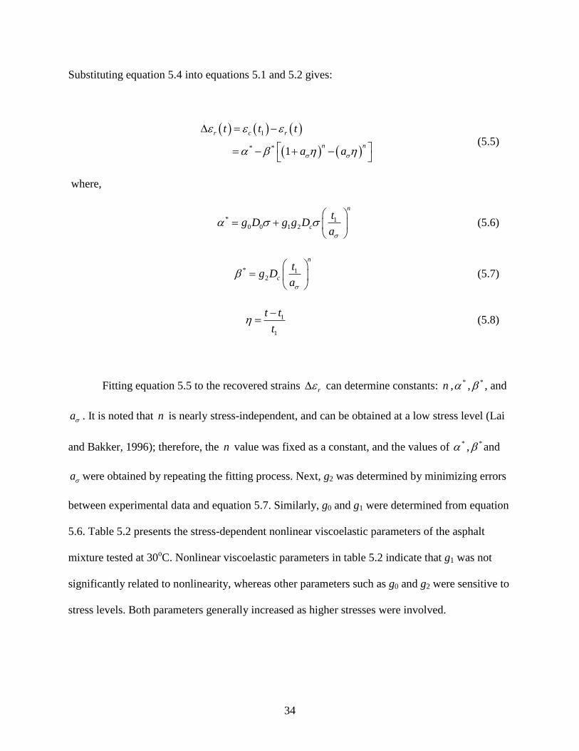
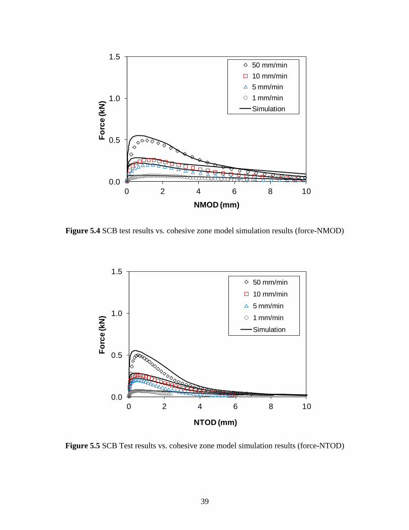
good match between test results and numerical simulations was observed. Figures 5.4 and 5.5
present good agreements between the test results (average of the three SCB specimens per case)
and finite element simulations. Resulting fracture properties (Tmax and Gc) at each loading rate
are presented in table 5.3. The good agreement between tests and model simulations indicates
that the local fracture properties were properly defined through the integrated experimental-
numerical approach.
Mesh & B.C. Deformed Mesh
Cohesive Zone Elements
Figure 5.3 A finite element modeling of the SCB testing
39
0.0
0.5
1.0
1.5
0 2 4 6 8 10
Fo
rce
(k
N)
NMOD (mm)
50 mm/min
10 mm/min
5 mm/min
1 mm/min
Simulation
Figure 5.4 SCB test results vs. cohesive zone model simulation results (force-NMOD)
0.0
0.5
1.0
1.5
0 2 4 6 8 10
Fo
rce
(kN
)
NTOD (mm)
50 mm/min
10 mm/min
5 mm/min
1 mm/min
Simulation
Figure 5.5 SCB Test results vs. cohesive zone model simulation results (force-NTOD)
40
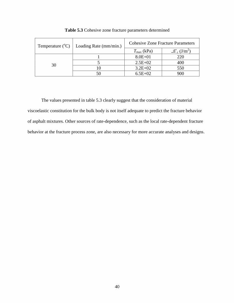
Table 5.3 Cohesive zone fracture parameters determined
Temperature (oC) Loading Rate (mm/min.)
Cohesive Zone Fracture Parameters
Tmax (kPa) Gc (J/m2)
30
1 8.0E+01 220
5 2.5E+02 400
10 3.2E+02 550
50 6.5E+02 900
The values presented in table 5.3 clearly suggest that the consideration of material
viscoelastic constitution for the bulk body is not itself adequate to predict the fracture behavior
of asphalt mixtures. Other sources of rate-dependence, such as the local rate-dependent fracture
behavior at the fracture process zone, are also necessary for more accurate analyses and designs.

41
Chapter 6 Finite Element Analysis of Pavement
In this chapter, a typical pavement structure used in Nebraska was modeled through the
2-D finite element method, in order to investigate the mechanical performance behavior of the
pavement when subjected to heavy truck loading. The 2-D finite element modeling was
conducted using a commercial package, ABAQUS Version 6.8 (2008), which was incorporated
with the cohesive zone fracture and the developed nonlinear viscoelastic UMAT. Simulation
results comparing responses from linear viscoelasticity and from the use of nonlinear viscoelastic
material characteristics with and without the cohesive zone fracture are presented and discussed
in this chapter.
6.1 Pavement Geometry and Boundary Conditions
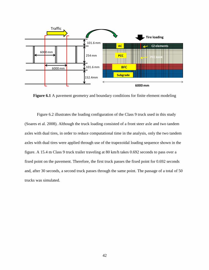
A typical pavement structure used in Nebraska was selected for simulations. Figure 6.1
illustrates a four-layered asphalt pavement structure (101.6 mm thick asphalt layer, 254 mm
Portland cement concrete (PCC) layer with PCC joints, 101.6 mm bituminous foundation course
(BFC) and 152.4 mm subgrade). Both sides of the vertical edge of the finite element pavement
model were fixed in the horizontal direction, and the bottom of the model was fixed in the
vertical direction to represent a rock foundation. To reduce computational time, graded meshes,
which have finer elements close to the potential separation/distress regions, were used (fig. 6.1).
The red line in the figure indicates the region where cohesive zone elements were inserted in the
mesh to allow cracking (reflective and/or top-down). A tire pressure of 720 kPa and axial load of
35.5 kN were applied to the pavement based on a study by Yoo (2007).
42
101.6 mm
254 mm
152.4mm
101.6 mm
Traffic
6000 mm
6000 mm
AC
PCC
Subgrade
CZ elements
PCC Joint
BFC
6000 mm
Tire loading
Figure 6.1 A pavement geometry and boundary conditions for finite element modeling
Figure 6.2 illustrates the loading configuration of the Class 9 truck used in this study
(Soares et al. 2008). Although the truck loading consisted of a front steer axle and two tandem
axles with dual tires, in order to reduce computational time in the analysis, only the two tandem
axles with dual tires were applied through use of the trapezoidal loading sequence shown in the
figure. A 15.4 m Class 9 truck trailer traveling at 80 km/h takes 0.692 seconds to pass over a
fixed point on the pavement. Therefore, the first truck passes the fixed point for 0.692 seconds
and, after 30 seconds, a second truck passes through the same point. The passage of a total of 50
trucks was simulated.

43
Time (sec)
Amplitude
0
1
0.058 0.634 0.692
Figure 6.2 Truck loading configuration (Class 9) used in this study
6.2 Layer Properties
Table 6.1 presents material properties of the individual layers. The underlying layers (i.e.,
PCC, BFC, and subgrade) were modeled as isotropic linear elastic, while viscoelastic response
was considered to describe the behavior of the asphalt concrete surface layer. The surface layer
can dissipate energy due to its viscoelastic nature and cohesive zone, which results in permanent
deformation (rutting) and fracture of the layer. Different performance responses between the
linear and nonlinear viscoelastic approaches with and without cohesive zone fracture were
130 cm 1280 cm
177.8cm
30.48cm
130 cm
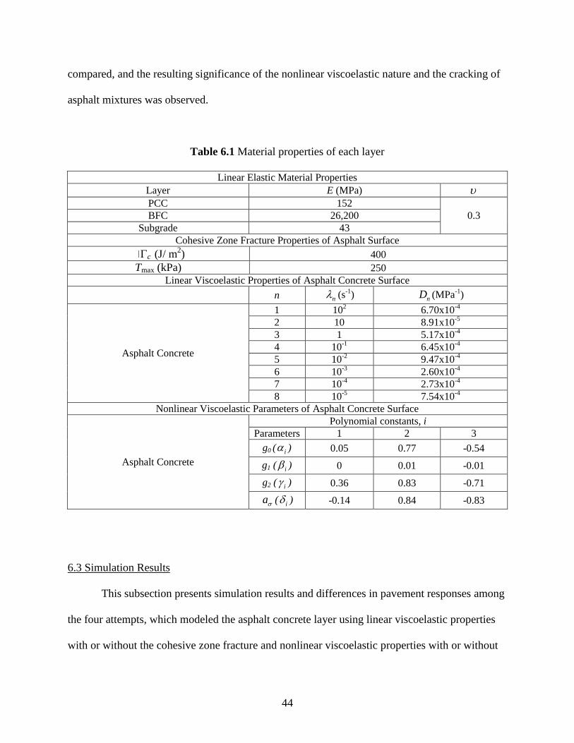
44
compared, and the resulting significance of the nonlinear viscoelastic nature and the cracking of
asphalt mixtures was observed.
Table 6.1 Material properties of each layer
Linear Elastic Material Properties
Layer E (MPa) PCC 152
0.3 BFC 26,200 Subgrade 43
Cohesive Zone Fracture Properties of Asphalt Surface
Gc (J/ m2) 400
Tmax (kPa) 250 Linear Viscoelastic Properties of Asphalt Concrete Surface
n n (s-1
) nD (MPa-1
)
Asphalt Concrete
1 102 6.70x10
-4 2 10 8.91x10
-5 3 1 5.17x10
-4 4 10
-1 6.45x10⁻⁴
5 10-2 9.47x10
-4 6 10
-3 2.60x10⁻⁴
7 10-4 2.73x10
-4 8 10
-5 7.54x10⁻⁴
Nonlinear Viscoelastic Parameters of Asphalt Concrete Surface
Asphalt Concrete
Polynomial constants, i Parameters 1 2 3
g0 ( i ) 0.05 0.77 -0.54
g1 ( i ) 0 0.01 -0.01
g2 ( i ) 0.36 0.83 -0.71
a ( i ) -0.14 0.84 -0.83
6.3 Simulation Results
This subsection presents simulation results and differences in pavement responses among
the four attempts, which modeled the asphalt concrete layer using linear viscoelastic properties
with or without the cohesive zone fracture and nonlinear viscoelastic properties with or without

45
the cohesive zone fracture behavior. Among many mechanical responses, the vertical
displacement from the pavement surface, the crack opening (horizontal) displacement through
the depth of the asphalt concrete layer, and the horizontal strain at the bottom of the asphalt layer
were examined with the 50 cycles of truck loading; they are strongly related to the two primary
distresses of asphaltic pavement: rutting and cracking.
6.3.1 Permanent Deformation (Rut Depth)
Figure 6.3 compares permanent deformation (rut depth) accumulated from each truck
loading up to the 50 cycles. It clearly shows the increasing difference in the rut depth among the
four cases as the number of loading cycles increases. At the end of the 50 cycle simulation, the
total rut depth predicted from the nonlinear viscoelastic with the cohesive zone fracture was the
greatest, while the rut depth simulated from the linear viscoelastic without cohesive zone was the
smallest. The figure clearly demonstrates the effects of material characteristics on the overall
pavement performance.
Figure 6.4 shows contour plots of vertical displacement distributions in the asphalt layer
for different numbers of loading cycles (i.e., 10, 30, and 50 cycles) obtained from the four
modeling approaches. Contour plots in the top left-hand-side are results from the simulation of
linear viscoelastic without cohesive zone fracture, while the top right-hand-side plots were
obtained in consideration of the cohesive zone fracture in the linear viscoelastic asphalt layer.
Similarly, contour plots in the bottom left-hand-side were from the simulation of nonlinear
viscoelastic without cohesive zone fracture, and the bottom right-hand-side plots present vertical
displacement contours resulting from model simulation with nonlinear viscoelasticity and
cohesive zone fracture of asphalt layer. These plots clearly show that vertical displacement from
the nonlinear viscoelastic model propagates much more quickly to the bottom of the asphalt layer
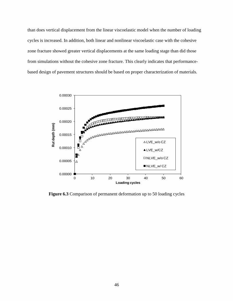
46
than does vertical displacement from the linear viscoelastic model when the number of loading
cycles is increased. In addition, both linear and nonlinear viscoelastic case with the cohesive
zone fracture showed greater vertical displacements at the same loading stage than did those
from simulations without the cohesive zone fracture. This clearly indicates that performance-
based design of pavement structures should be based on proper characterization of materials.
0.00000
0.00005
0.00010
0.00015
0.00020
0.00025
0.00030
0 10 20 30 40 50 60
Ru
t d
ep
th (
mm
)
Loading cycles
LVE_w/o CZ
LVE_w/CZ
NLVE_w/o CZ
NLVE_w/ CZ
Figure 6.3 Comparison of permanent deformation up to 50 loading cycles

47
LVE w/ CZ
NLVE w/ CZ
LVE w/o CZ
NLVE w/o CZ
(a) at 10th cycle
LVE w/ CZ
NLVE w/ CZ
LVE w/o CZ
NLVE w/o CZ
(b) at 30th cycle
Figure 6.4 Contour plots of vertical displacement distributions

48
LVE w/ CZ
NLVE w/ CZ
LVE w/o CZ
NLVE w/o CZ
(c) at 50th cycle
Figure 6.4 Contour plots of vertical displacement distributions (cont’d.)
6.3.2 Horizontal Strain
Figure 6.5 shows horizontal strain profiles at the bottom of the asphalt layer for up to 50
truck loading cycles. Note that the sign convention adopted herein is positive for tension. As
shown in the figure, the maximum tensile strains take place below the tire, and compressive
strains develop between the tires. The nonlinear viscoelastic model predicted greater maximum
tensile strains than did the case of linear viscoelastic layer. Regarding the effect of cohesive zone
fracture on the horizontal strain at the bottom of the asphalt layer, smaller horizontal strains were
monitored from the cases without cohesive zone fracture behavior than from cases with cohesive
zones for both linear viscoelastic and nonlinear viscoelastic models.

49
-5.00E-05
0.00E+00
5.00E-05
1.00E-04
1.50E-04
2.00E-04
2.50E-04
3.00E-04
0 1000 2000 3000 4000 5000 6000 7000
Ho
rizo
nta
l S
train
Distance (mm)
N=50 for LVE_w/o CZ
N=50 for LVE_w/ CZ
(a) linear viscoelasticity simulations
-5.00E-05
0.00E+00
5.00E-05
1.00E-04
1.50E-04
2.00E-04
2.50E-04
3.00E-04
0 1000 2000 3000 4000 5000 6000 7000
Ho
rizo
nta
l S
train
Distance (mm)
N=50 for NLVE_w/o CZ
N=50 for NLVE_w/ CZ
(b) nonlinear viscoelasticity simulations
Figure 6.5 Comparison of horizontal strain plots
50
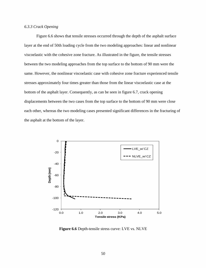
6.3.3 Crack Opening
Figure 6.6 shows that tensile stresses occurred through the depth of the asphalt surface
layer at the end of 50th loading cycle from the two modeling approaches: linear and nonlinear
viscoelastic with the cohesive zone fracture. As illustrated in the figure, the tensile stresses
between the two modeling approaches from the top surface to the bottom of 90 mm were the
same. However, the nonlinear viscoelastic case with cohesive zone fracture experienced tensile
stresses approximately four times greater than those from the linear viscoelastic case at the
bottom of the asphalt layer. Consequently, as can be seen in figure 6.7, crack opening
displacements between the two cases from the top surface to the bottom of 90 mm were close
each other, whereas the two modeling cases presented significant differences in the fracturing of
the asphalt at the bottom of the layer.
-120
-100
-80
-60
-40
-20
0
0.0 1.0 2.0 3.0 4.0 5.0
Dep
th (m
m)
Tensile stress (KPa)
LVE_w/ CZ
NLVE_w/ CZ
Figure 6.6 Depth-tensile stress curve: LVE vs. NLVE

51
-120
-100
-80
-60
-40
-20
0
0.00E+00 5.00E-06 1.00E-05 1.50E-05 2.00E-05 2.50E-05 3.00E-05
Dep
th (m
m)
crack opening (mm)
LVE_w/ CZ
NLVE_w/ CZ
Figure 6.7 Depth-crack opening curve: LVE vs. NLVE

52
Chapter 7 Summary and Conclusions
As an extension of Ban et al. (2011), we have sought a more advanced constitutive model
for asphalt mixtures, in order to more accurately predict pavement responses. To this end,
Schapery’s nonlinear viscoelastic constitutive model was implemented into the commercial finite
element software ABAQUS via a user defined subroutine (UMAT), and the cohesive zone
fracture model was involved in the process to more realistically analyze distresses in asphaltic
pavements subjected to heavy truck loads. Several laboratory tests (i.e., creep-recovery tests at
various stress levels to obtain stress-dependent viscoelastic material properties; semi-circular
bending (SCB) fracture tests at different loading rates to identify viscoelastic fracture properties)
of an asphalt mixture were conducted. Test results were used to obtain fundamental material
properties, which were in turn used to model structural performance of a typical Nebraska
asphaltic pavement.
Detailed investigations of the pavement responses resulting from different constitutive
relations (i.e., linear viscoelastic and nonlinear viscoelastic with and without cohesive zone
fracture) provided interesting observations and findings that could be used to better understand
the effects of truck loading on pavement damage, and consequently to further advance current
pavement-analysis design methods. The following bullet points summarize the conclusions that
can be drawn:
Schapery’s nonlinear viscoelastic model was well implemented into the ABAQUS via a user
material subroutine UMAT. An example problem presented in this study verified the model
and its numerical implementation.
53
Creep-recovery tests at varying stress levels were conducted to identify viscoelastic mixture
characteristics. As expected, test results clearly demonstrated stress-dependent mixture
characteristics.
Utilizing the creep-recovery test results, a series of processes was applied to identify linear
and nonlinear viscoelastic properties. Linear viscoelastic properties were characterized by the
Prony series based on the generalized Maxwell model, and nonlinear viscoelastic parameters
were successfully fitted to polynomial functions, which enables the representation of
individual nonlinear viscoelastic properties as a continuous function of stress levels.
At intermediate service temperatures such as 30oC, the rate-dependent fracture behavior was
obvious. Cohesive zone fracture properties varied as the loading rate changed.
Two-dimensional finite element simulations of a pavement structure showed significant
differences among the cases (linear viscoelastic vs. nonlinear viscoelastic with and without
fracture damage) in the prediction of pavement performance (both rutting and cracking).
Although test results and numerical simulations presented in this study are limited in their
ability to make definitive conclusions, performance differences observed between individual
cases are considered significant and should be addressed in the process of performance-based
pavement design. These findings imply the necessity of deliberate, accurate, and more
realistic characterizations of paving materials.
54
References
Airey, G., B. Rahimzadeh, and A. C. Collop. 2004. “Linear rheological behavior of bituminous
paving material.” Journal of Materials in Civil Engineering, 16: 212–220.
American Association of State Highway and Transportation Officials (AASHTO). 2008.
Mechanistic-empirical pavement design guide, Interim edition: A manual of practice.
Available from https://bookstore.transportation.org
Al-Qadi, I. L., M .A. Elseifi, and P. J. Yoo. 2004. “In-situ validation of mechanistic pavement
finite element modeling.” Proceedings of the 2nd International Conference on
Accelerated Pavement Testing, Minneapolis, MN.
Al-Qadi, I. L., A. Loulizi, I. Janajreh, and T. E. Freeman. 2002. “Pavement response to dual
and new wide base Tires at the same tire pressure.” Transportation Research Record,
1806: 38-47.
Al-Qadi, I. L., P. J. Yoo, and M .A. Elseifi. 2005. “Characterization of pavement damage due to
different tire configurations.” Journal of the Association of Asphalt Paving Technologists,
74 : 921-962.
Aragão, F. T. S. 2011. “Computational microstructure modeling of asphalt mixtures subjected to
rate-dependent fracture.” Ph.D. Diss., University of Nebraska, Lincoln.
Aragão, F. T. S. and Y. Kim. 2011. “Characterization of fracture properties of asphalt
mixtures based on cohesive zone modeling and digital image correlation technique.”
Transportation Research Board 2011 Annual Meeting, Washington, D.C.
Bazant, Z.P. and J. Planas. 1998. Fracture and size effect in concrete and other quasibrittle
materials. Boca Raton, FL: CRC Press.
Blab, R., and J. T. Harvey. 2002. “Modeling measured 3D tire contact stresses in a viscoelastic
FE pavement model.” International Journal of Geomechanics, 2, no. 3: 271-290.
Collop, A. C., A. Scarpas, C. Kasbergen, and A. Bondt. 2003. “Development and finite element
implementation of stress-dependent elastoviscoplastic constitutive model with damage
for asphalt.” Transportation Research Record, 1832 : 96-104.
Dassault Systemes SIMULIA Ltd. 2008. ABAQUS. Version 6.8. Available from wwwl.3ds.com
Duan, K., X. Hu, and F. H. Wittmann. 2006. “Scaling of quasi-brittle fracture: Boundary and
size effect.” Mechanics of Materials, 38: 128-141.
Elseifi, M. A., and I. L. Al-Qadi. 2006. “Modeling of strain energy absorbers for rehabilitated
cracked flexible pavements.” Journal of Transportation Engineering, 131, no. 9: 653-
661.

55
Elseifi, M. A., I. L. Al-Qadi, and P. J. Yoo. 2006. “Viscoelastic modeling and field validation
of flexible pavements.” Journal of Engineering Mechanics, 132, no. 2: 172-178.
Espinosa, H.D. and P. D. Zavattieri. 2003. “A grain level model for the study of failure initiation
and evolution in polycrystalline brittle materials, Part I: Theory and numerical
implementation.” Mechanics of Materials, 35: 333-364.
Geubelle, P. and J. Baylor, J. 1998. “Impact-induced delamination of laminated composites: A
2D simulation.” Composites Part B – Engineering, 29, no. 5: 589-602.
Haji-Ali, R. and A. Muliana. 2004. “Numerical finite element formulation of the Schapery
non-linear viscoelastic material model.” International Journal for Numerical Methods
in Engineering, 59: 25-45.
Huang, C. W., R. K. Abu Al-Rub, R. K., E. A. Masad, and D. N. Little. 2011. “Three-
dimensional simulations of asphalt pavement permanent deformation using a nonlinear
viscoelastic and viscoplastic model.” Journal of Materials in Civil Engineering, 23, no. 1:
56-68.
Kim, Y., D. H. Allen, D. H., and D. N. Little. 2007. “Computational constitutive model for
predicting nonlinear viscoelastic damage and fracture failure of asphalt concrete
mixtures.” International Journal of Geomechanics 7, no. 2: 102-110.
Kim, Y., D. H. Allen, and G. D. Seidel. 2006. “Damage-induced modeling of elastic-
viscoelastic randomly oriented particulate composites.” Journal of Engineering
Materials and Technology, 126 : 18-27.
Kim, Y., H. Ban, H., and S. Im. 2011. “Impact of truck loading on design and analysis of
asphaltic pavement structures-Phase II.” MATC Final Report No. MATC-UNL 321,
Lincoln, Nebraska.
Kim, H. and W. G. Buttlar. 2009. “Discrete fracture modeling of asphalt concrete.”
International Journal of Solids and Structures, 46: 2593-2604.
Kim, Y. R., J. S. Daniel, and H. Wen, H. 2002. “Fatigue performance evaluation of WestTrack
asphalt mixtures using viscoelastic continuum damage approach.” Final Report No.
FHWA/NC/2002-004, North Carolina State University.
Kim, K. W., S. J. Kweon, Y. S. Doh, and T. S. Park. 2003. “Fracture toughness of polymer-
modified asphalt concrete at low temperatures.” Canadian Journal of Civil Engineering,
30: 406-413.
Kim, H., M. P. Wagoner, and W, G. Buttlar. 2008. “Simulation of fracture behavior in asphalt
concrete using a heterogeneous cohesive zone discrete element model.” Journal of

56
Materials in Civil Engineering, 20, no. 8: 552-563.
Lai, J. and A. Bakker. 1996. “3-D Schapery representation for non-linear viscoelasticity and
finite element implementation.” Computational Mechanics, 18: 182-191.
Li, X. and Marasteanu, M. O. (2005). “Cohesive Modeling of Fracture in Asphalt Mixtures at
Low Temperatures.” International Journal of Fracture, 136, 285-308.
Li, X. and M. O. Marasteanu. 2010. “The fracture process zone in asphalt mixture at low
temperature.” Engineering Fracture Mechanics, 77: 1175-1190.
Marasteanu, M. O., A. Zofka, M. Turos, X. Li, R. Velasques, X. Li, W. Buttlar, G. Paulino, A.
Braha, E. Dave, J. Ojo, H. Bahia, C. Williams, J. Bausano, A, Gallistel, and L.
McGraw. 2007. “Investigation of low temperature cracking in asphalt pavements:
National pooled fund study 776.” Final Report No. MN/RC 2007-43, Minnesota
Department of Transportation.
Masad, E., and N. Somadevan. 2002. “Microstructural finite-element analysis of influence of
localized strain distribution of asphalt mix properties.” Journal of Engineering
Mechanics, 128: 1105–1114.
Mobasher, B., M. Mamlouk, and H. Lin. 1997. “Evaluation of crack propagation properties of
asphalt mixtures.” Journal of Transportation Engineering, 123, no. 5: 405–413.
Mull, M. A., K. Stuart, and A. Yehia. 2002. “Fracture resistance characterization of chemically
modified crumb rubber asphalt pavement.” Journal of Materials Science, 37: 557-566.
Mun, S., M. Guddati, and Y. R. Kim. 2004. “Fatigue cracking mechanisms in asphalt
pavements with viscoelastic continuum damage finite element program.”0
Transportation Research Record, 1896: 96-106.
Schapery, R. A. 1969. “On the Charcaterization of Nonlinear Viscoelastic Materials.” Polymer
Engineering and Science, 9: 295-310.
Seo, Y., Y. R. Kim, and M. W. Witczak. 2002. “Application of the digital image correlation
method to mechanical testing of asphalt-aggregate mixtures.” Transportation Research
Record, 1789: 162-172.
Soares, R. F., D. H. Allen, Y. Kim, C. Berthelot, J. B. Soares, J. B., and M. E. Rentschler. 2008.
“A computational model for predicting the effect of tire configuration on asphaltic
pavement life.” International Journal on Road Materials and Pavement Design, 9, no. 2:
271-289.
Song, S. H., G. H. Paulino, and W. G. Buttlar. 2006. “A bilinear cohesive zone model tailored
for fracture of asphalt concrete considering viscoelastic bulk material.” Engineering
Fracture Mechanics, 73, no. 18: 2829-2847.
57
Song, S. H., M. P. Wagoner, and G. H. Paulino. 2008. “δ25 crack opening displacement
parameter in cohesive zone models: Experiments and simulations in asphalt concrete.”
Fatigue and Fracture of Engineering Materials and Structures, 31: 850-856.
Wagoner, M. P., W. G. Buttlar, and G. H. Paulino. 2005. “Development of a single-edge notched
beam test for asphalt concrete mixtures.” Journal of Testing Evaluation, 33, no. 6: 452–
460.
Wagoner, M. P., W. G. Buttlar, and G. H. Paulino. 2005. “Disk-shaped compact tension test for
asphalt concrete fracture.” Society for Experimental Mechanics, 45, no. 3: 270–277.
Yoo, P. J. 2007. “Flexible pavement dynamic responses analysis and validation for various
tire configurations.” PhD Diss., University of Illinois at Urbana-Champaign.
Zhao, Y. 2002. “Permanent deformation characterization of asphalt concrete using a
viscoelasticplastic model.” PhD Diss., North Carolina State University.