report # matc-unl: 054 final...
TRANSCRIPT

®
The contents of this report reflect the views of the authors, who are responsible for the facts and the accuracy of the information presented herein. This document is disseminated under the sponsorship of the Department of Transportation
University Transportation Centers Program, in the interest of information exchange. The U.S. Government assumes no liability for the contents or use thereof.
Alternative Funding Mechanisms forState Transportation Systems in Predominantly Rural States
Report # MATC-UNL: 054 Final Report
John E. Anderson, Ph.D.ProfessorDepartment of EconomicsUniversity of Nebraska-Lincoln
Eric Thompson, Ph. D. Associate Professor
2014
A Coopertative Research Project sponsored by U.S. Department of Tranportation-Research, Innovation and Technology Innovation Administration
WBS:25-1121-0003-054

Alternative Funding Mechanisms for State Transportation Systems in Predominantly Rural States
John E. Anderson, Ph.D. Professor Department of Economics University of Nebraska-Lincoln Eric Thompson, Ph.D. Associate Professor Department of Economics University of Nebraska-Lincoln
A Report on Research Sponsored by
Mid-America Transportation Center
University of Nebraska-Lincoln
January 2014

ii
Technical Report Documentation Page 1. Report No. 25-1121-0003-054
2. Government Accession No.
3. Recipient's Catalog No.
4. Title and Subtitle Alternative Funding Mechanisms for State Transportation Systems in Predominantly Rural States
5. Report Date January 2014
6. Performing Organization Code
7. Author(s) Eric Thompson and John E. Anderson
8. Performing Organization Report No. 25-1121-0003-054
9. Performing Organization Name and Address Mid-America Transportation Center 2200 Vine St. PO Box 830851 Lincoln, NE 68583-0851
10. Work Unit No. (TRAIS) 11. Contract or Grant No.
12. Sponsoring Agency Name and Address Research and Innovative Technology Administration 1200 New Jersey Ave., SE Washington, D.C. 20590
13. Type of Report and Period Covered July 2012 – December 2013
14. Sponsoring Agency Code MATC TRB RiP No. 32777
15. Supplementary Notes
16. Abstract The Transportation Research Board of the National Academies has identified a number of research needs related to alternative transportation finance systems. Alternatives are needed because motor fuels taxes are proving to be insufficient to fund operation and maintenance costs of the transportation system. The long-term trend is likely to be continuing use of motor fuel taxes, supplemented by, or transitioning to, use-based fees. Current research in progress in this area is focused on designing variable fees that will internalize congestion externalities in urban areas. These approaches are particularly well suited to highly urbanized areas, but other approaches may be required for predominantly rural states. One possible approach is to implement an optimal two-part tariff, which incorporates a flat fee with a variable charge. Such a two-part tariff is an efficient solution in markets with increasing returns to scale and falling long-run average cost curves. Efficiency requires pricing at the marginal cost of travel, and given low marginal costs in rural areas (with limited congestion), a flat fee is needed in combination with the variable charge, in order to make the financing mechanism sustainable. The current transportation funding system already includes flat fees (licensing and registration fees) and variable fees (gasoline and diesel taxes). The researchers' approach is to consider alternative configurations of these two existing mechanisms, which in combination may be capable of mimicking an optimal two-part tariff. The research will be carried out utilizing data from the state of Nebraska on licensing and registration fees and taxes by type of vehicle, motor fuels tax revenues by source, and data on average annual daily travel (AADT), as well as engineering estimates of road maintenance costs associated with automobile and truck travel. 17. Key Words
18. Distribution Statement
19. Security Classif. (of this report) Unclassified
20. Security Classif. (of this page) Unclassified
21. No. of Pages 68
22. Price

iii
Table of Contents Disclaimer ...................................................................................................................................... vi Abstract ......................................................................................................................................... vii Chapter 1 Introduction and Background ..........................................................................................1 Chapter 2 Review of Fuel Elasticity Estimates ................................................................................8 Chapter 3 Two-Part Tariffs ............................................................................................................16 Chapter 4 Empirical Evidence .......................................................................................................20 Chapter 5 Review of State and Local Taxes and Fees ...................................................................29
1.1 Nebraska Case Study ...................................................................................................32 Chapter 6 Summary, Conclusions, and Recommendation.............................................................40 References ......................................................................................................................................43 Appendix A ....................................................................................................................................46 Appendix B ....................................................................................................................................57 1.1 Model ...........................................................................................................................57 1.2 Effect of Various Taxes (comparative static analysis) ................................................59

iv
List of Figures Figure 1.1 Taxes as a Share of Retail Price, monthly data 2000.1-2013.3 ......................................4 Figure 3.1 Marginal Cost Pricing in the Presence of Increasing Returns to Scale ........................17 Figure 3.2 Congestion Cost Pricing ..............................................................................................19 Figure 5.1 Annual Motor Vehicle Registration Fees by State, 2012 .............................................32 Figure 5.2 State and Local Gasoline Tax (cents per gallon), 2012 ................................................32 Figure 5.3 Nebraska Transportation Funding ...............................................................................39

v
List of Tables Table 1.1 Components of Retail Gasoline Prices, 2013 ..................................................................4 Table 1.2 Funding Gap Analysis for Selected Texas Road Segments .............................................5 Table 1.3 Share of State and Local Road Spending Covered by Fuel Taxes, Tolls, and Other User Taxes and Fees: MTC States, 2010 ...........................................................6 Table 2.1 Summary of Gasoline Price Elasticity Studies ..............................................................10 Table 2.2 Price and Income Elasticities by Household Characteristics .........................................11 Table 2.3 Welfare Change Relative to Expenditure for an Increase in the Gasoline Excise Tax ..........................................................................................................12 Table 2.4 Nebraska Motor Fuels Revenue Elasticity Estimation, 2007-2012 ...............................14 Table 4.1 Pavement and External Costs per Mile by Vehicle Type in Urban and Rural Areas:
2013 Estimates ...................................................................................................................22 Table 4.2 Annualized Construction and Maintenance Costs per Mile for Rural Highways ..........26 Table 4.3 Annualized Construction and Maintenance Costs per Mile for Rural Highways ..........27 Table 4.4 Gross and Net Fixed Costs per Mile of Rural Highway ...............................................28 Table 5.1 Nebraska Department of Roads FY 2013 Receipts ($ thousands) .................................38 Table 5.2 Nebraska Department of Roads FY 2013 Operating Expenditures ($ thousands) ........38

vi
Disclaimer
The contents of this report reflect the views of the authors, who are responsible for the
facts and the accuracy of the information presented herein. This document is disseminated under
the sponsorship of the U.S. Department of Transportation’s University Transportation Centers
Program, in the interest of information exchange. The U.S. Government assumes no liability for
the contents or use thereof.

vii
Abstract
The Transportation Research Board of the National Academies has identified a number of
research needs related to alternative transportation finance systems. Alternatives are needed
because motor fuels taxes are proving to be insufficient to fund operation and maintenance costs
of the transportation system. The long-term trend is likely to be continuing use of motor fuel
taxes, supplemented by, or transitioning to, use-based fees. Current research in progress in this
area is focused on designing variable fees that will internalize congestion externalities in urban
areas. These approaches are particularly well suited to highly urbanized areas, but other
approaches may be required for predominantly rural states. One possible approach is to
implement an optimal two-part tariff, which incorporates a flat fee with a variable charge. Such a
two-part tariff is an efficient solution in markets with increasing returns to scale and falling long-
run average cost curves. Efficiency requires pricing at the marginal cost of travel, and given low
marginal costs in rural areas (with limited congestion), a flat fee is needed in combination with
the variable charge, in order to make the financing mechanism sustainable. The current
transportation funding system already includes flat fees (licensing and registration fees) and
variable fees (gasoline and diesel taxes). The researchers' approach is to consider alternative
configurations of these two existing mechanisms, which in combination may be capable of
mimicking an optimal two-part tariff. The research will be carried out utilizing data from the
state of Nebraska on licensing and registration fees and taxes by type of vehicle, motor fuels tax
revenues by source, and data on average annual daily travel (AADT), as well as engineering
estimates of road maintenance costs associated with automobile and truck travel.

1
Chapter 1 Introduction and Background
This research study is in response to the Transportation Research Board (TRB) of the
National Academies, which identified a number of research needs related to alternative
transportation finance systems. As motor fuel taxes on both gasoline and diesel fuel—the
primary source of current funding—are proving to be insufficient to fund the operation and
maintenance costs of transportation systems, alternatives are needed. The long-term trend is
likely to be the continued use of motor fuel taxes, supplemented by or transitioning to alternative
use-based fees.
Current research in progress in this area is focused on designing variable fees that will
internalize congestion externalities in urban areas. Tolls and their collection via new
technologies are a particular set of options that has drawn much attention. Various types of fees
based on vehicle miles travelled (VMT) are also receiving serious consideration. While
congestion tolls and VMT charges are feasible financing mechanisms to consider, they are
particularly well-suited to highly urbanized areas. Receiving less attention is the particular set of
circumstances of predominantly rural states. In these states, the problem of the inadequacy of
motor fuels taxes is just as pressing, but the problem to be solved is not congestion. Small
populations and tax bases, aging infrastructure, rising costs, and pressing needs for economic
development characterize many areas of these states. The fundamental problem is how to pay for
the maintenance and operation of the road network with the declining resources provided by
motor fuels taxes.
One possible approach is to implement an optimal two-part tariff which incorporates a
flat fee with a variable charge. In markets with increasing returns to scale and falling long-run
average cost curves, a two-part tariff is an efficient solution. Efficiency requires pricing at the
2
marginal cost of travel, but in an economic setting with economies of scale, as exists in the
transportation sector, such pricing does not cover the full cost of providing and maintaining the
road network in a rural setting. Hence, a flat fee is needed in combination with the variable
charge in order to make the financing mechanism sustainable. Such mechanisms are feasible
given the current methods of charging network users. Currently, car and truck operators pay both
annual licensing fees (or taxes) and motor fuel taxes. The licensing fee is a flat charge, and the
motor fuels tax is a variable charge based on road usage. Our approach is to consider alternative
configurations of these two existing mechanisms, which in combination may be capable of
mimicking an optimal two-part tariff.
This research addresses two of the United States Department of Transportation’s strategic
goals: (1) improving the state of good repair, and (2) improving economic competitiveness.
Appropriate adoption of two-part tariffs can improve the state of good repair by assuring the
provision of a more reliable source of revenue for transportation agencies. This will also have the
benefit of improving economic competitiveness by moving toward a taxation system that better
matches variable tax (i.e., motor fuels tax) rates to the marginal cost imposed by vehicle usage in
relatively uncongested settings.
We simulate alternative financing mechanisms for predominantly rural states in this
study, with special reference to Region VII states, including Missouri, Iowa, Nebraska, and
Kansas. While each state is home to significant metropolitan areas, these states are also
characterized by large geographic areas and relatively small populations, making for low density
regions served by extended road networks. We also simulate several variants of optimal two-part
tariffs.

3
Crane et al (2011) indicate that, “The key failure of current gasoline and diesel taxes is
that revenues have not kept pace with the cost of building and maintaining federally funded
highways, nor have they covered the external costs associated with oil.” The later issue of
external costs associated with oil is beyond the scope of the present study, but the former issue is
at the heart of the road funding problem currently faced by predominately rural states. Within the
Region VII states of Missouri, Iowa, Nebraska, and Kansas, the road funding issue is viewed as a
predicament, as reflected in the report of the Platte Institute (2013).
Figure 1.1 illustrates the clear national trend of fuel taxes as a share of the retail price of
gasoline declining over the past decade. Taxes comprised approximately 20% of the retail price
in the early 2000s, but have subsequently fallen to less than five percent. Of course, the major
reason that the ratio of taxes to retail price has fallen is that taxes are generally defined as unit
taxes with the rate defined in cents per gallon. As the retail price of gasoline has risen, the taxes
have remained fixed in value, causing the ratio to fall. Most recently, gasoline prices have
moderated, and as a result, taxes as a share of the retail price have risen again.

4
Figure 1.1 Taxes as a Share of Retail Price, monthly data 2000.1-2013.3
Source: authors’ computation based on U.S. Energy Information Administration data.
Table 1.1 illustrates the components of the retail price of gasoline in October 2013.
Federal and state excise taxes on gasoline accounted for 13%of the retail price at that time
(reflecting the most recent data available from the U.S. Energy Information Administration).
Table 1.1 Components of Retail Gasoline Prices, 2013
Components of Retail Price: Percent of Retail Price ($3.34/gallon, October 2013)
Crude Oil 71% Refining costs and profits 5% Distribution, marketing, and retail costs and profits 11% Federal and state taxes 13%
Source: U.S. Energy Information Administration, retrieved from: www.eia.gov/tools/faqs/faq.cfm?id=22&t=10
Reuben and Shadunsky (2012) state that, “Since the early 1990s, gasoline prices have
been increasing. … At the same time, vehicle fleets are getting more fuel efficient and
consequently our existing gasoline taxes are raising less revenue.” An important consequence of
0
5
10
15
20
25
30
35
4020
00.1
2000
.520
00.9
2001
.120
01.5
2001
.920
02.1
2002
.520
02.9
2003
.120
03.5
2003
.920
04.1
2004
.520
04.9
2005
.120
05.5
2005
.920
06.1
2006
.520
06.9
2007
.120
07.5
2007
.920
08.1
2008
.520
08.9
2009
.120
09.5
2009
.920
10.1
2010
.520
10.9
2011
.120
11.5
2011
.920
12.1
2012
.520
12.9
2013
.1
Taxes as a share of retail price, 2000.1-2013.3

5
the improving efficiency of the motor vehicle fleet and moderation in the demand for fuel as
prices rise is that tax revenue declines.
Cambridge Systematics Inc. (2008) was commissioned by the Texas Department of
Transportation to conduct an analysis of the so-called “highway construction equity gap”—the
difference between tax and fee revenues associated with specific roads and the construction and
maintenance costs associated with those roads. Their analysis for seven sample road segments in
Texas is summarized in table 1.2.
Table 1.2 Funding Gap Analysis for Selected Texas Road Segments Road Segment Revenue/Cost State MFT rate required for
R = C ($/gal) 1: Austin—US 183 South of US 290 to North Bolm Road 0.32 1.85
2: Brownsville—US 277 Relief Rout around Del Rio 0.14 4.64 3: Dallas-Fort Worth—IH-820 from Southwestern
Railroad (DART) to SH26 0.31 1.77
4: El Paso—IH-10 from LP 375 (Transmountain Road) to SH 20 (Mesa Street)
0.93 0.28
5: Houston—Harris Perland FM 865 from Beltway 8 South to FM 518
0.13 4.93
6: San Antonio—FM 3487 from IH-410 to FM 471; FM 2696 from Glade Crossing to West Oak Estates; Spur 421
from Ligistrum to IH-10
0.37 1.50
7: Longview—Tyler Loop 281 from 0.96 miles south of SH 300 to US 259
0.21 2.82
Source: Cambridge Systematics Inc. (2008)
Revenues from federal motor fuels taxes together with state revenues from motor fuels
taxes and vehicle registration fees cover between 13%-93% of construction costs. The 2008
study also computed the state motor fuels tax rate that would be required on each road segment
in order to assure that revenues equaled costs. The required state tax rates ranged from $0.28/gal
to $4.93/gal, and varied inversely with the share of costs covered by existing federal and state
revenues. In addition, Henchman (2013a, 2013b) has estimated the share of state and local road
spending covered by fuel taxes, tolls, and other user taxes and fees.

6
Table 1.3 reports Henchman’s (2013a, 2013b) estimates for the Midwest Transportation
Center states. The data indicate that taxes and fees cover between 19%-32%of state and local
road spending, and a somewhat higher percentage of total transportation spending. Even when
state shares of federal spending are included, as illustrated in the right-hand side of table 1.3, the
shares covered by taxes and fees are within the range of 42% to 54%.
Table 1.3 Share of State and Local Road Spending Covered by Fuel Taxes, Tolls, and Other
User Taxes and Fees: MTC States, 2010 State Percent of State
and Local Road Spendinga
Rank Percent of State and Local Total Transportation
Spendinga
Rank Percent of State and Local Road
Spending, Including Federal Gasoline
Taxb
Rank
Iowa 19.4 46 21.5 44 53.8 20 Kansas 29.8 27 30.3 32 47.7 27 Missouri 22.9 38 28.0 36 42.3 38 Nebraska 31.8 19 43.1 7 42.2 39 Notes: (a) Numerator is state and local spending on roads, excluding federal aid; denominator includes state and local spending financed by federal aid. (b) Numerator is state and local spending on roads, including that financed by federal and state motor fuel tax revenue plus state highway revenue; denominator includes state and local spending financed by federal aid. Source: Henchman (2013a, 2013b).
These data are illustrative of the fundamental problem that excise taxes levied per gallon
of fuel together with other forms of tolls and fees are unlikely to be insufficient to provide
sufficient financing for current levels of road construction and maintenance activity in states.
Alternatives to the traditional excise tax on gasoline have been suggested, as in Totty
(2012). Suggestions include taxing VMT, taxing road use with tolls, switching fuel taxes from
unit taxes to ad valorem taxes, taxing oil rather than gasoline, and taxing automobiles. While
Totty and others have made such suggestions for the federal fuel excise tax replacement, several
of these ideas are applicable at the state level as well. For predominantly rural states, two of
these ideas are particularly relevant: switching fuel taxes from unit taxes to ad valorem taxes,
and taxing automobiles.

7

8
Chapter 2 Review of Fuel Elasticity Estimates
In this section the authors investigate how sensitive fuel demand may be in response to
changes in the price of fuel. It is critical to determine this relationship this for two reasons: first,
this information will facilitate a better knowledge of how fuel demand is likely to fall in the
future as fuel prices rise, thereby causing fuel tax revenue based on the number of gallons of fuel
sold to decline. Second, by attaining this information, ad valorem tax rates to replace the unit tax
rates currently applied to fuels can be more accurately recommended.
The sensitivity of gasoline demand to changes in gasoline price is measured by the price
elasticity of demand. This elasticity is defined as the percent change in quantity demanded
divided by the percent change in price. If the ratio is less than (one in absolute value), demand is
said to be inelastic. In that circumstance, a given change in price results in a less-than-
proportionate response in quantity demanded, indicating that consumers are not highly
responsive to the price change.
The demand for gasoline has been estimated in a number of studies over the years, with
general results found in the literature evidencing that demand is price inelastic. For example, a
meta-analysis in Brons, Nijkand and Teitveld (2008) reported an overall short-run price elasticity
of -0.34. This estimate indicates that a 10% increase in price was associated with a 3.4%
reduction in quantity demanded. Table 2.1 reports price elasticity estimates from a number of
recent studies, all of which indicate that short-run elasticity is low (i.e., substantially less than
unity, which would reflect a proportional response).
The importance of these price elasticity estimates is that any increase in the price of
gasoline will result in a reduction in the quantity of gasoline demanded, but a less than
proportionate reduction. Two tax implications follow. First, the quantity of gasoline falls, which

9
results in a reduction in tax revenue if the gasoline tax is a unit tax applied with a rate expressed
in cents per gallon. Second, expenditure on gasoline rises, which results in an increase in tax
revenue if the gasoline tax is an ad valorem tax applied with a rate expressed as a percentage of
the price.

10
Table 2.1 Summary of Gasoline Price Elasticity Studies
Study Study Characteristics Scope of Study Price Elasticity Estimates Goodwin, Dargay, and Hanly (2004)
Summarized various fuel price and income elasticity studies
1929 to 1991 North America and Europe
-0.25 short run -0.6 long run
Espey (1996) 101 fuel price elasticity studies
1936-1986 U.S. -0.26 short run -0.58 long run
Glaister and Graham (2002) Review of various fuel price and elasticity studies
1950-2000 North America -0.2 to -0.3 short run -0.6 to -0.8 long run
Lipow (2008) Review of selected elasticity studies
1950- 2000 North America and Europe
-0.17short run -0.4 long run
Small and Van Dender (2005)
Comprehensive model using state level cross sectional time series of gasoline price elasticities
U.S. Data 1996- 2001 1996 to 2001: -0.09 short run -0.41 long run 1997 to 2001: -0.07 short run -0.34 long run
Hymel, Small, and Van Dender (2010)
Comprehensive model using state-level cross sectional time series of gasoline prices
1966- 2004 U.S. Data -0.055 short run -0.285 long run
Agras and Chapman (2001) Gasoline price elasticity 1982-1995 U.S. Data -.25 short run -.92 long run
Li, Linn, and Muehlegger (2011)
Comprehensive model with tax increases and price fluctuations analyzed separately
1968-2008 U.S. Data -0.235 long run
Hughes, Knittle, and Sperling (2006)
Comprehensive model using state-level cross-sectional time series gasoline prices
1975-2006 U.S. data 1975-1980 -0.21 to -.34 short run 2001-2006 -0.034 to -0.077 short run
Komanoff (2008) Simple model of short run fuel price elasticities
2004 to 2011 U.S. data -0.04 in 2004 short run -0.08 in 2005 short run -0.12 in 2006 short run -0.16 in 2007 short run -0.29 in 2011 short run
Spiller and Stephens (2012) Comprehensive model of monthly state level fuel price and vehicle miles traveled data
2009 U.S. travel survey data
-.67 short run with variations by household income and location
Long-run price elasticities are larger in absolute value, reflecting the fact that, given a
longer time period over which to adjust, households are more responsive to gasoline prices. Even
so, the long-run elasticity estimates are still less than one. Over a period of time long enough that

11
households are able to alter their vehicle ownership—perhaps trading an older, fuel-inefficient
vehicle for a newer, more efficient vehicle—their gasoline consumption is more responsive to
price than in the short run. It is possible, however, that with a more efficient vehicle, the
household may decide to drive more, thereby reducing the expected impact on gasoline
consumption. In the transportation literature, there is a so-called “rebound effect,” as in Litman
(2012, 2013), which captures this aspect of the change in demand in response to price.
Elasticity estimates also vary with household characteristics, as reported in Wadud,
Graham, and Noland (2010a) and Wadud, Noland, and Graham (2010b) and summarized in table
2.2. Modeling heterogeneity among households results in estimates that differ based on a wide
variety of characteristics, including income, the number of vehicles in the household, the
presence of multiple wage earnings in the household, and other factors. Most important for the
present study, their estimates reveal that rural households have smaller price elasticites than do
urban households. That general result indicates that rural households are less responsive to
changes in gasoline prices. The lack of alternative modes of transportation and fixed commuting
patterns are likely reasons for the less elastic demand among rural households.
Table 2.2 Price and Income Elasticities by Household Characteristics
Source: Wadud, Graham and Noland (2010a).
Household Characteristics Elasticity Estimates
Location Car ownership
Wage earners Price and income elasticities computed at national average
Price and income elasticitities computed at group average
Price Income Price income Urban Single Zero/one -0.341 0.273 -0.414 0.329 Urban Single Multiple -0.425 0.314 -0.401 0.304 Urban Multiple Zero/one -0.493 0.373 -0.484 0.365 Urban Multiple Multiple -0.577 0.414 -0.490 0.351 Rural Single Zero/one -0.091 0.297 -0.236 0.391 Rural Single Multiple -0.175 0.338 -0.238 0.362 Rural Multiple Zero/one -0.243 0.397 -0.325 0.445 Rural Multiple Multiple -0.327 0.438 -0.321 0.423

12
Income elasticity estimates are also of interest, as they reflect how gasoline consumption
varies with household income levels. It has been well known since Poterba (1991) that gasoline
excise taxes are progressive at the lower end of the income distribution, but become regressive at
higher income levels. At the low end of the income distribution there are many households that
do not own vehicles; hence, gasoline excise taxes do not fall directly on these households. At
higher levels of income, however, vehicle ownership rises, and excises taxes as a share of
income also rise. Wadud, Graham, and Noland (2010a) provide recent estimates of the welfare
impact of an increase in the excise tax, summarized in table 2.3.1 Their estimates were computed
both for all households and vehicle-owning households. For all households, the welfare impact
rose over the first three deciles of the income distribution, but fell thereafter. Considering only
vehicle-owning households, however, the welfare impact monotonically decreased with income,
with higher income households experiencing a smaller welfare reduction.
Table 2.3 Welfare Change Relative to Expenditure
for an Increase in the Gasoline Excise Tax
All Households Vehicle-Owning Households
Decile 1 (lowest) -3.47 -5.37 Decile 2 -3.87 -4.89 Decile 3 -4.13 -4.64 Decile 4 -4.11 -4.47 Decile 5 -3.84 -4.03 Decile 6 -3.63 -3.77 Decile 7 -3.42 -3.52 Decile 8 -2.98 -3.06 Decile 9 -2.61 -2.66 Decile 10 (highest) -1.57 -1.59 Rural -4.35 -4.41
Source: Wadud, Graham, and Noland (2010a).
1 The tax increase simulated in Wadud, Graham, and Noland (2010a) was $1.10 per gallon, which was the amount computed by Parry and Small (2005) as the tax required to internalize the external costs associated with gasoline.
13
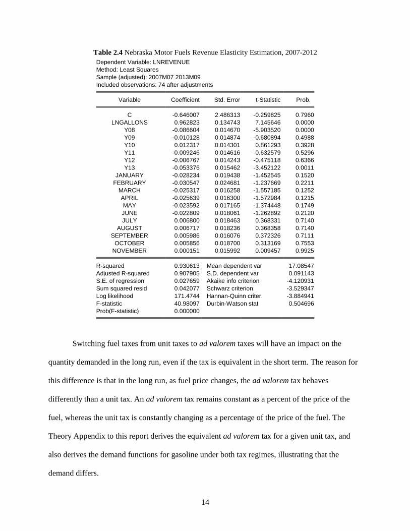
Another elasticity to consider is the revenue elasticity of motor fuels sold. Table 2.4
reports the estimation of a statistical model of Nebraska motor fuels tax revenue using monthly
data over the period of July 2007-September 2013. The model explains variations in the natural
logarithm of motor fuels revenue as a function of the natural logarithm of the number of gallons
of motor fuel sold, along with control variables for monthly and yearly trends (2007 is the left-
out year in the model). The revenue elasticity was estimated as 0.96, which was not statistically
different from one. This is precisely what would be expected when tax rates are expressed as unit
taxes applied in cents-per-gallon. Revenue is proportionate to gallons sold. This model illustrates
the weakness of defining motor fuels taxes as unit taxes in the context of rising fuel prices and
falling demand.
14
Table 2.4 Nebraska Motor Fuels Revenue Elasticity Estimation, 2007-2012 Dependent Variable: LNREVENUE Method: Least Squares Sample (adjusted): 2007M07 2013M09 Included observations: 74 after adjustments
Variable Coefficient Std. Error t-Statistic Prob. C -0.646007 2.486313 -0.259825 0.7960
LNGALLONS 0.962823 0.134743 7.145646 0.0000 Y08 -0.086604 0.014670 -5.903520 0.0000 Y09 -0.010128 0.014874 -0.680894 0.4988 Y10 0.012317 0.014301 0.861293 0.3928 Y11 -0.009246 0.014616 -0.632579 0.5296 Y12 -0.006767 0.014243 -0.475118 0.6366 Y13 -0.053376 0.015462 -3.452122 0.0011
JANUARY -0.028234 0.019438 -1.452545 0.1520 FEBRUARY -0.030547 0.024681 -1.237669 0.2211
MARCH -0.025317 0.016258 -1.557185 0.1252 APRIL -0.025639 0.016300 -1.572984 0.1215 MAY -0.023592 0.017165 -1.374448 0.1749 JUNE -0.022809 0.018061 -1.262892 0.2120 JULY 0.006800 0.018463 0.368331 0.7140
AUGUST 0.006717 0.018236 0.368358 0.7140 SEPTEMBER 0.005986 0.016076 0.372326 0.7111
OCTOBER 0.005856 0.018700 0.313169 0.7553 NOVEMBER 0.000151 0.015992 0.009457 0.9925
R-squared 0.930613 Mean dependent var 17.08547
Adjusted R-squared 0.907905 S.D. dependent var 0.091143 S.E. of regression 0.027659 Akaike info criterion -4.120931 Sum squared resid 0.042077 Schwarz criterion -3.529347 Log likelihood 171.4744 Hannan-Quinn criter. -3.884941 F-statistic 40.98097 Durbin-Watson stat 0.504696 Prob(F-statistic) 0.000000
Switching fuel taxes from unit taxes to ad valorem taxes will have an impact on the
quantity demanded in the long run, even if the tax is equivalent in the short term. The reason for
this difference is that in the long run, as fuel price changes, the ad valorem tax behaves
differently than a unit tax. An ad valorem tax remains constant as a percent of the price of the
fuel, whereas the unit tax is constantly changing as a percentage of the price of the fuel. The
Theory Appendix to this report derives the equivalent ad valorem tax for a given unit tax, and
also derives the demand functions for gasoline under both tax regimes, illustrating that the
demand differs.
15
The primary benefit of switching motor fuels taxes from unit taxes to ad valorem taxes is
to maintain the rate of tax in relation to the price of fuel rather than the number of gallons cleared
in the market. In an era of rising fuel prices and falling demand for fuel, this tax policy change
can help preserve the revenues necessary for maintaining current levels of road building and
ongoing road maintenance.

16
Chapter 3 Two-Part Tariffs
A common financing method used in industries subject to increasing returns to scale due
to high fixed network costs is the two-part tariff (TPT). This financing mechanism combines the
advantageous effect of pricing network use at marginal cost, which results in the efficient use of
the network, together with a flat network access fee that in the aggregate covers the long-run cost
of building and maintaining the network. The TPT funding mechanism has been used most
extensively in the field of public utilities, especially electric utilities, but has also been used in a
wide variety of other industries, from mass transit systems to health clubs.2
The economics of roads are based on the fundamental fact that the long-run average cost
curve (LRAC) is downward-sloping due to the high fixed cost of road construction. Given that
the LRAC is falling, it must be the case that the marginal cost (MC) is not only also falling, but
must be below the LRAC. In such a situation, the usual efficiency rule to price road services at
MC will fail to generate sufficient revenue to cover the cost of the road. Figure 3.1 illustrates this
situation.
In the illustration in Figure 3.1, a perfectly elastic demand is assumed for simplicity,
illustrated as a horizontal line. As a result, the demand curve is also the marginal revenue curve
(MR) and the average revenue curve (AR). If we follow the usual efficient pricing rule and price
road use at p = MC in order to obtain the efficient amount of road use, the revenue generated will
be the rectangle 0q1ab. The total cost of providing q1 units of road services is the rectangle
0q1cd. With this pricing scheme, total cost exceeds the revenue generated by the rectangle abcd.
Hence, marginal cost pricing results in a deficit in the road fund. In such a situation, the desirable
2 Notable papers on two-part tariffs include Bormann (2003), Brito et al (2010), Hoernig and Valletti (2011), Jensen (2008), Mitomo (2001), Naughton (1986), Oi (1971), and Shaffer (1992).

17
marginal cost pricing rule, taken from a perfectly competitive market context, will not work in
the sense that the financing is insufficient to cover the cost of the road in the long run. One
solution to this problem is to subsidize the road from general revenues. Another potential
solution is to implement a two-part tariff.
Figure 3.1 Marginal Cost Pricing in the Presence of Increasing Returns to Scale
With a two-part tariff we can achieve the desired efficient result, but not generate a
deficit that must be financed from general revenues. Road users must pay two fees. The first fee
is a subscription fee equal to one road user’s share of the deficit abcd. Second, there must be a
variable fee charged per road trip. This two-part tariff can be thought of as a linear price,
𝑝 = 𝑎 + 𝑏𝑞, where the price p is a flat fee a plus a variable fee bq, which depends on the number
of trips q and the per-trip charge b. In the road context, it is easiest to think of the variable charge
as being based on the excise tax revenue collected from gasoline or diesel fuel taxes. The flat fee
can be viewed as a type of registration fee, motor vehicle fee, or other type of annual charge per
vehicle (e.g., wheel tax).
LRAC
a
d
MC
D, MR, AR
$
Output, q 0
b
c
q1

18
Our empirical strategy is to first obtain estimates from the transportation literature on the
MC and LRAC of building and maintaining roads for both automobile and commercial truck use,
as illustrated in Figure 3.1. With these estimates we can then design the TPT, with the variable
component of size aq1 and the fixed component of size ad. Financing the entire system then
requires setting per trip or per mile variable fees based on gasoline and diesel fuel taxes at aq1 to
generate a total revenue of 0q1ab, and designing flat fees at ad per vehicle to generate total a
revenue of abcd. The combination of the two components of the TPT then generates sufficient
revenue to cover the long-run total cost of the road network.
A second important perspective is provided as we consider the effects of congestion.
Figure 3.2 illustrates the cost per mile to the driver, with the driver’s MC and AC initially
constant at the level MC1. As the number of vehicles on the road increases, however, congestion
costs arise beginning with V* vehicles per mile of roadway. Beyond that level of road use, the
MC exceeds AC as travel time is lengthened due to the congestion cost externality. At low levels
of demand, such as Demand 1, there is no congestion cost to consider, and pricing the trip at MC
is efficient. If demand is greater, however, as illustrated with Demand 2, then the uncontrolled
equilibrium volume V2 is inefficient because there is too much congestion. The objective of a toll
mechanism is to move to equilibrium volume V2’ through a toll pricing mechanism. Since
demand indicates the willingness of drivers to pay, the objective is to match that willingness to
pay with the marginal cost of trips, including the congestion cost.
In terms of pricing travel, this situation can also call for a two-part tariff approach. The
basic fee per trip is set at MC1, which can be implemented with a gasoline excise tax, among
other possibilities. The second component of the TPT is designed to internalize the congestion
externality. A toll can be implemented for this purpose. In predominantly rural areas, congestion

19
costs are not a major issue, however. Hence, our focus is not on congestion tolls, but rather on
the TPT financing mechanism to assure that the long-run average cost of roads can be
appropriately covered.
Figure 3.2 Congestion Cost Pricing
Average Cost
Marginal Cost
Traffic volume V* V1 V2
Trip cost ($)
MC1
Demand 1
Demand 2
V2’

20
Chapter 4 Empirical Evidence
The marginal costs of highway travel are primarily composed of a variety of fuel,
depreciation, maintenance and other costs borne by vehicle users. However, there are a number
of “external” costs borne by others. Examples of external costs include congestion or pollution.
Take the example of congestion. As traffic increases on a road, each additional vehicle
which utilizes the road has an influence on the trip of other vehicles. In particular, each
additional vehicle adds to traffic, causing other vehicles to drive more slowly or haltingly. As a
result, on a congested road, each vehicle which chooses to use a road not only faces their own
costs (such as the cost of gasoline), but also imposes costs on other drivers. Pollution is another
example where drivers impose costs on others. Automobiles utilizing an internal combustion
engine emit pollutants with each mile driven. Electric cars also may pollute for each mile driven
when the required electricity is generated at power plants that utilize fossil fuels. The safe
disposal of batteries may be another concern. These examples, where vehicle drivers impose
costs on others, are known as “externalities.”
As the examples above note, there is reason to believe that external costs may be lower
for vehicles operating in a rural area. Vehicles driving on lightly-traveled rural roads are less
likely to impose the types of congestion externalities described above. The roads are present
since there is a need to connect smaller towns with transportation access; but the roads may be
lightly traveled, and therefore at most times and during most days a vehicle using the road has
little impact on travel costs for other vehicles, e.g., speed, consistency of speed, or risk of
accident. This is true even though the lane capacity of rural roads is generally lower than the lane
capacity of urban roads. Similarly, air pollution in a rural area may not lead as frequently to
health problems given that that 1) there is less density of pollution (or more air to absorb the

21
pollution) and 2) there are fewer people around to be impacted by pollution. The external costs
of travel therefore are likely to be low per mile traveled in a rural area.
Wear and tear on the road is a different case—it is a cost for the road owner rather than
for other vehicles. Wear and tear on the road, therefore, cannot be considered an externality from
travel. However, wear and tear costs are among the marginal costs of vehicle travel which are not
born by the vehicle user and are measured below. Wear and tear costs also differ substantially
between classes of vehicles. In particular, the maintenance costs imposed by each additional mile
traveled are much higher for heavy commercial trucks than for automobiles and light trucks.
Further, trucks, due to their size and relatively slow travel, can generate substantially different
congestion costs in some situations. Pollution levels also may differ between heavy trucks and
automobiles and light trucks due to the lower miles per gallon and different types of fuels found
among trucks.
The authors conducted a review of literature to identify external and other marginal costs
imposed by automobile and truck operators. Estimates were developed both for rural and urban
areas. Among the research examined, the most comprehensive data was available in the
Addendum to the 1997 Federal Cost Highway Allocation Study. That study focused on interstate
travel, but also provided information on pavement, congestion, external crash costs, air pollution
and noise pollution costs for rural and urban vehicles of different size classes for the year 2000.
Unfortunately, the Federal Highway Administration has not updated that study, though the
primary external costs, such as congestion costs and air pollution, have remained problems in the
intervening years. Road damage requiring repaving also remains a concern. As a result, cost data
from the year 2000 was updated to 2013 to reflect the intervening increase in costs. The cost
update was completed using the Consumer Price Index.

22
The 1997 Federal Cost Highway Allocation Study also included two additional classes of
external marginal costs from vehicle travel. These were external crash costs and noise pollution.
External crash costs include costs imposed beyond the accident victims and their insurers.
Examples include the cost for police in securing, protecting, and investigating an accident scene,
or costs for other travelers who are delayed because of an accident. Noise pollution costs are
primarily a concern for trucks within urban areas.
Table 4.1 compares road maintenance (i.e., “pavement”) costs per mile of travel as well
as the four classes of external costs: congestion, crash, air pollution, and noise pollution costs for
automobiles and trucks. Costs are presented in the tables for 60-kip 5-axle combination trucks.
Automobiles and light trucks are both included in the automobile category. As noted previously,
costs were updated to 2013 values, and are presented for interstates located in both urban and
rural areas.
Table 4.1 Pavement and External Costs per Mile by Vehicle Type in Urban and Rural Areas:
2013 Estimates
Cents/Mile Automobiles 60 Kip 5-Axle Combination Trucks Rural Urban Rural Urban Pavement Costs 0.00 0.14 4.47 14.21 Congestion Costs 1.06 10.42 2.54 24.88 Crash Costs 1.33 1.61 1.19 1.56 Air Pollution 1.54 1.80 5.21 6.08 Noise Pollution 0.01 0.12 0.23 3.72 Total 3.94 14.09 13.64 50.44
Results in table 4.1 show the stark difference in the marginal pavement and external costs
imposed by automobiles and combination trucks, and between vehicles traveling in rural and
urban areas. Costs per mile for crashes and air pollution are similar between urban and rural
areas, while crash costs also are similar between cars and trucks. Air pollution costs, however,
23
are three times higher for trucks in both urban and rural areas, reflecting the lower mileage for
trucks.
Noise pollution and pavement costs were primarily problems for trucks, particularly in
urban areas. The costs of wear and tear on pavement were nearly three times higher for trucks
operating in urban areas than rural areas. Pavement damage from heavy vehicles rises quickly
with the volume of traffic, as the repeat incidence of weight is especially damaging for
pavement. Noise pollution is worse for trucks, but costs are only high in urban areas where there
are many people to hear the noise and where homes are located directly adjacent to highways.
Noise pollution costs for trucks operating in urban areas averaged 3.72 cents per mile in 2013
dollars.
The primary reason for the difference in the pavement and external costs of travel
between urban and rural areas is congestion costs. Congestion costs are naturally higher in urban
areas, where each additional vehicle utilizing a roadway imposes a larger external cost.
Congestion costs were 10.42 cents per mile for automobiles and 24.88 cents per mile for trucks.
Stated another way, congestion costs were the largest cost component in urban areas, accounting
for 60% of marginal costs for automobiles operating in urban areas and nearly 50% of marginal
costs for trucks operating in urban areas.
Results confirm the well-known result that the marginal external and pavement costs of
truck travel is substantially higher than for auto travel. This implies that it would make greater
economic sense to impose higher marginal travel costs on heavy trucks than on automobiles and
light trucks. However, it is also evident in table 4.1 that marginal costs are substantially lower in
rural areas than in urban areas for both automobiles and trucks. For automobiles, most of that
difference in cost is due to lower congestion costs. For trucks, differences in congestion costs

24
remain the primary reason for higher costs in urban areas, but differences in pavement costs and
noise pollution per mile traveled also contribute.
How large are the differences? For automobiles, the marginal external and pavement
costs of travel is just 3.94 cents per mile on rural interstates versus 14.09 cents per mile on urban
interstates. For trucks, the marginal external and pavement costs is 13.64 cents per mile in rural
areas and 50.44 cents per mile in urban areas. Results suggest that marginal taxes on driving,
such as those implied by the tax on motor fuels should be substantially higher for trucks than
automobiles, and for vehicles operating in urban areas rather than rural areas. Flat fees for both
automobiles and trucks, which are not related to miles traveled, should account for a larger share
of revenue in rural areas.
Whatever the marginal costs of travel, another issue is the fixed costs of providing
highways from construction and maintenance, and what share of this fixed cost is covered by
fuel tax revenues. This section considers the share of highway fixed costs in rural areas that can
be covered by the fuel tax collected from automobiles and commercial trucks at current tax rates.
Remaining fixed costs would need to be covered by alternative sources of funding. The analysis
proceeds by calculating and comparing the annualized construction plus maintenance costs for
one mile of rural road, and then comparing that cost to the annualized fuel tax revenue from
automobiles and commercial trucks driving on that mile of road.
Life-cycle analysis is a common methodology that has been used to compare the fixed
costs of highway segments (construction and maintenance) with the fuel tax revenue generated
by cars driving on those segments.3 The life-cycle cost estimates the total construction, regular
3 Cambridge Systematics, Inc., 2008. The Highway Construction Equity Gap, Prepared for the Texas Department of Transportation, Government and Public Affairs Division (February).

25
maintenance, and reconstruction of pavement over an extended “life” of a highway segment,
typically a period of 30 to 40 years. These fixed costs over a lifetime are then based on
projections of lifetime fuel tax revenue, which are based on projections of average annual daily
traffic (AADT) and fuel efficiency for cars and trucks over the lifetime of the highway.
Such a life-cycle approach, however, requires projections about future AADT, vehicle
mileage, fuel tax rates, and even the types of vehicles that will be in use (electric vs. hybrid vs.
internal combustion) over decades into the future. For this section of our larger report, the
authors plan to use a much more straightforward approach based on current, measureable values
for costs, AADT, vehicle mileage, and fuel tax rates. Our approach calculates the annualized cost
of new construction and annual maintenance costs, and compares that with the fuel tax revenues
generated from estimates of current AADT on rural highways.
Table 4.2 shows the annualized construction costs and maintenance costs per mile for
rural highways. Estimates are shown for the two most common types of highways found in rural
areas. The most common are two-lane arterial roads that go between many of the smaller
communities in a rural state. Another common type of highway is the four-lane divided highway
found in select rural areas within states; for example, the state of Nebraska has built hundreds of
miles of four-lane divided highway in rural counties as part of its expressway system.
Construction and maintenance cost estimates come from averages maintained by state highway
agencies around the country. Construction cost estimates are from Arkansas, Florida and the
consulting service CapitolFax. Maintenance cost estimates are from Texas. As can be seen, the
total annual cost is $117,200 for two-lane arterial highways and $227,600 for four-lane divided
highways.

26
Table 4.2 Annualized Construction and Maintenance Costs per Mile for Rural Highways
Category two-lane arterial four-lane divided Construction Costs Per Mile $2,565,000 $4,957,000 Annualized 25-Year Lifespan $102,600 $198,300 Annual Maintenance Costs $14,600 $29,300 Total Annualized Cost Per Mile $117,200 $227,600
Source: Arkansas State Highway and Transportation Agency, Florida Department of Transportation, CapitolFax, and Texas Department of Transportation.
Table 4.3 shows an estimate of potential fuel tax revenue for each type of highway.
Estimates are based on traffic patterns on rural Nebraska highways. Results represent an average
of AADT on non-interstate highways in 10 randomly selected rural and five randomly selected
micropolitan counties in the state. The first row of Table 4.3 shows the average AADT, or
average daily traffic on rural Nebraska highways. The table represents the number of cars and
trucks that pass a particular spot on a highway on average over the course of a day. The AADT
results therefore can be considered as an estimate of the total number of vehicles that drive on a
mile of road during a particular day. The second row of Table 4.3 multiplies the AADT by 365 to
provide an estimate of the number of automobiles or commercial trucks that drive on a mile of
road on two-lane arterial or four-lane divided highways over the course of a year.
The next question pertains to how much fuel is consumed by automobiles or commercial
trucks driving over the average mile of a two-lane arterial or four-lane divided highway. This is
estimated by utilizing the average vehicle miles per gallon for the automobile (including light
trucks) and commercial truck fleets. The estimated average fuel efficiency is 21.4 miles per
gallon based on the average fuel efficiency of short-axle light duty vehicles (passenger cars -
67% weight) and long-axle light duty vehicles (light trucks - 33% weight) reported by the U.S.

27
Department of Transportation in 2010, the most recent year available. An average of six miles
per gallon is used for commercial trucks. This calculation is seen in the third and fourth rows of
Table 4.3.
Annual fuel usage per mile of road is then multiplied by the total state and federal fuel
tax per gallon for gasoline (automobiles) and diesel (commercial trucks) to estimate the fuel tax
revenue generated by each mile of highway over a year. According to the American Petroleum
Institute, the total state and local fuel tax is $0.456 per gallon for gasoline in Nebraska, and
$0.510 per gallon for diesel. 4 While federal fuel tax revenue is not automatically returned to the
state where it is generated, most federal tax revenue is returned to the states. As a result, it is
appropriate to include the federal revenue as a source generating revenue for Nebraska. The
average mile of two-lane arterial highway yields a fuel tax revenue of $9,700 each year from
automobiles and $6,700 from trucks. The annual total is $16,400. For a four-lane divided
highway, the fuel tax revenue per mile was $42,800 each year from automobiles and $37,000 per
mile from trucks. The annual total is $79,900.
Table 4.3 Annualized Construction and Maintenance Costs per Mile for Rural Highways
two-lane arterial four-lane divided Category Automobiles Trucks Automobiles Trucks AADT 1,245 216 5,509 1,193 AAAT (AADT X 365) 454,380 78,755 2,010,890 435,394 Vehicle Miles Per Gallon 21.4 6 21.4 6 Estimated Gallons Per Mile Per Year 21,233 13,126 93,967 72,566 Fuel Tax Per Gallon $0.456 $0.510 $0.456 $0.510 Estimate Revenue Per Mile Per Year $9,682 $6,694 $42,849 $37,009 Combined Total Autos and Trucks $16,376 $79,857
Source: Author’s calculations
4 American Petroleum Institute, State Motor Fuels Taxes, revised October 8, 2003.

28
Table 4.4 compares the annualized fixed costs per mile of rural highway to the expected
annual fuel tax revenue generated by that mile of highway. Table 4.4 also shows the fixed costs
per mile that is not covered by fuel tax revenue and must be covered by some other revenue
source. All costs and revenues are rounded to thousands of dollars. The annual uncovered fixed
costs were $101,000 per mile for two-lane arterials, or 86% of fixed costs. The annual uncovered
fixed costs were $148,000 per mile for four-lane divided highway, or 65% of fixed costs.
Table 4.4 Gross and Net Fixed Costs per Mile of Rural Highway
Category two-lane arterial four-lane divided Total Annual Fixed Cost Per Mile $117,000 $228,000 Total Annual Fuel Tax Revenue Per Mile $16,000 $80,000 Fixed Costs Uncovered Per Mile $101,000 $148,000 Percentage of Fixed Costs Uncovered 86% 65%
Source: Author’s calculations

29
Chapter 5 Review of State and Local Taxes and Fees
States apply a variety of taxes and fees to motor vehicles, but the general pattern is to
have an excise tax on gasoline and diesel fuel, a sales tax applied at the point of vehicle sale, an
annual registration fee, and some form of annual tax or fee determined by vehicle value or
weight, or both. State and local gasoline excise taxes in 2012 are illustrated in figure 5.2. These
taxes are generally applied as unit taxes where the tax rate is expressed in cents per gallon of
fuel. The combined total of state and local taxes varies widely across states. The EIA reports
that the average state motor gasoline tax on January 1, 2013, was 23.47 cents per gallon, while
the federal tax was 18.40 cents per gallon. But, figure 5.2 illustrates that when combined with
local taxes permitted in many states, the total state and local tax rates in the highest taxed state
exceeded 40 cents per gallon, as in California, Connecticut, Hawaii, Illinois, and New York. The
lowest state and local combined tax rates were in Alaska.
Based on the analysis in the Theory Appendix, if we wish to replace a current unit tax
with an ad valorem tax that has the same immediate impact on gasoline demand, the ad valorem
tax should be set equal to the ratio of the unit tax divided by the price of gasoline. For example,
the average state unit tax of 23.47 cents per gallon of gasoline, at the October 2013 average price
of $3.34/gal, could be replaced with an ad valorem tax of 7%. At this rate there would be no
immediate impact on the demand for gasoline and no impact on revenue generated. In the future,
as the price of gasoline increases, the ad valorem tax rate would maintain revenues in proportion
to the price of gasoline.
Some states also apply the state sales tax to gasoline and diesel fuel. Those states include
California (2.25% applied to gasoline, 9.42% applied to diesel fuel; local sales taxes also
applied), Connecticut (7% gross earnings tax applied), Georgia (4% prepaid state tax applied),
30
Hawaii (4% gross income tax), Illinois (6.25% sales tax), Indiana (7% sales tax), Michigan (6%
sales tax), New Jersey (4% gross receipts tax), New York (8 cents per gallon state sales tax plus
local sales taxes applied), Virginia (2% sales tax applied in areas where mass transit systems
exist), and Vermont (Motor Fuels Transportation Infrastructure Assessment fee is applied with a
rate on gasoline that varies quarterly and a 3 cent per gallon rate applied to diesel fuel). In
addition, several states have local option taxes that apply to motor fuels, including Florida,
Hawaii, and Nevada. In those states the local option sales tax revenue is sometimes dedicated to
local roads and transit systems, but in other cases it simply provides local general fund revenues.
The second broad category of taxes and fees applied to automobiles covers legal titles
and registration. Title fees are generally one-time fixed dollar amounts. Registration fees are
annual and are generally based on weight, age, or vehicle value. Figure 5.1 illustrates the annual
motor vehicle registration fees by state in 2012. California, Iowa, and Montana have the highest
fees of approximately $200 per vehicle. Utah and Wyoming are in a second tier fee level of
approximately $150 per vehicle. A number of states apply fees in the $100 per vehicle range,
including Alaska, Illinois, Michigan, North Dakota, and Oklahoma. The remaining states apply
fees of lesser amounts. In some cases, the fees are minimal, as in Arizona, Georgia, Indiana,
Louisiana, Minnesota, Mississippi, and South Carolina.
Appendix 1 reports the results of our comprehensive review of current state and local
taxes and fees for automobiles and motorcycles. The first set of columns report sales and use
taxes applied to automobiles at the time of purchase. The second set of columns report title and
registration fees for both automobiles and motorcycles, as well as fees for duplicates and special
plates. Finally, the last set of columns provides information on annual motor vehicle taxes.

31
Sales and use taxes applied to the purchase of automobiles generally follow the state
application of sales tax to other goods. Local option sales taxes are also applied where
applicable. In some cases, however, the tax is graduated and rises with either the purchase price
of the automobile or its weight. In those cases higher priced or heavier vehicles pay higher tax
rates. The taxes in this broad category of sales taxes go by various names, including: excise tax,
one-time registration fee, motor vehicle usage tax, highway use fee, etc.
The final category of taxes applied to motor vehicles is the annual property tax, or some
variant of an ad valorem tax or fee based on value. Determination of the taxable value of the
vehicle varies widely across the states with many based on a straight line depreciation scale
starting with purchase price or manufacturer’s suggested retail price (MSRP).
Commercial trucks that travel across many states within the U. S. are required to register
in a base state. In addition, registration fees are apportioned to the various states in which the
commercial trucks travel. For commercial motor carriers in the U. S. and Canada, the
International Registration Plan (IRP) provides a payment mechanism by which the motor carriers
can pay registration fees to the several states in which their trucks travel. License and
registration fees are apportioned to the base state and additional states across which the trucks
travel in proportion to mileage in each state.

32
Figure 5.1 Annual Motor Vehicle Registration Fees by State, 2012
Source: National Conference of State Legislatures (NCSL)
Figure 5.2 State and Local Gasoline Tax (cents per gallon), 2012
Source: National Conference of State Legislatures (NCSL)
1.1 Nebraska Case Study
Figure 5.3 illustrates Nebraska transportation financing in the form of a flow chart.
Motor fuels and special fuels taxes generated a total of 26.3 cents per gallon as of July 1, 2013.
Of that amount, 7.5 cents per gallon are dedicated to the Nebraska Department of Roads
(NDOR). Cities and counties receive unit taxes in the amount of 2.8 cents per gallon. Five

33
percent of the wholesale price of fuels (based on a six-month average, adjusted semi-annually) is
allocated as follows: Department of Roads 66%, cities 17%, and counties 17%. This ad valorem
tax was equivalent to a unit tax of 14.4 cents per gallon (an implicit wholesale price per gallon of
$2.88) on July 1, 2013. An additional 1.6 cents per gallon was applied as a variable component
of the state tax. The total state excise tax was 26.3 cents per gallon. In addition, Nebraska
allocates 85% of the revenue generated by an earmarked one-quarter of 1% of the general fund
state sales tax revenue to the State Highway Capital Improvement Fund (State Statute 39-2703).
Table 5.1 reports the Nebraska Department of Roads (NDOR) receipts for FY 2013.
NDOR receives approximately half of its revenue from state funds and the other half from
federal funds. State receipts amounted to $378.7 million of the total (49.5%) while federal
receipts amounted to $363.2 million (47.5 percent) of total receipts. The major source of state
receipts comes from state motor fuels taxes, which account for 58.4% of total state NDOR
receipts. The second largest source of state receipts is motor vehicle sales taxes, which
contribute 26.5% of the state total. Registration fees are minimal and contribute just 10% of the
total state receipts. The sales tax on the purchase price of vehicles required to be registered is
applied at the state rate of 5.5%, with 5% going to the State Highway Trust Fund and the
remaining .5% going to the Highway Allocation Fund. Motor vehicle registration fees ($15 per
passenger car and fees on other vehicles) go into the State Highway Trust Fund and the
Recreation Road Fund.
Table 5.2 reports the Nebraska Department of Roads operating expenditures for FY 2013.
Highway maintenance accounts for 15.8% of total expenditures while construction accounts for
74% of the total. State motor fuels revenue accounts for 32.2% of the combined expenditures on
highway road construction and maintenance. If federal receipts are netted out of combined

34
maintenance and construction expenditures, the remainder not covered by the present state motor
fuels taxes is $102.9 million. Much of that remainder ($100.5 million) is currently covered by
the state motor vehicle sales tax. This sales tax is like the flat fee portion of the two-part tariff in
figure 3.1, given that it does not depend on the number of miles that a vehicle travels.5 Vehicle
registration is another flat fee, though it raises just $37.9 million per year. These results indicate
that the majority of revenue raised in Nebraska comes from the variable portion of the two-part
tariff, specifically, the state and federal tax on motor fuels.
The current allocation between variable and fixed costs makes sense if the motor vehicle
tax is effectively charging drivers the marginal cost of their travel in terms of required road
maintenance, congestion, third-party accident costs, and pollution per mile traveled. Estimates of
these marginal costs are reported in figure 4.1. Starting with the results for rural automobiles and
light trucks, the marginal cost of travel from these sources is $0.0394 per mile. Given average
mileage of 21.4 miles per gallon for rural automobiles and light trucks, the estimated marginal
cost per gallon would be $0.843 per gallon. This cost is very similar to the marginal cost of
trucks operating on rural highways, which is $0.845 per gallon, based on a marginal cost of
$0.141 per mile and six miles per gallon. These per gallon marginal costs are the same order of
magnitude as the per gallon fuel tax that is charged in Nebraska. The combined state and federal
tax for gasoline is $0.456 per gallon for gasoline and $0.510 per gallon for diesel. While
marginal costs are higher, these estimates are derived from national averages, and factors such as
congestion and pollution costs may not be as high in Nebraska as for the average rural highway.
5 An inefficiency of the sales tax is that it generates greater revenue from more expensive vehicles even if the costs imposed by automobiles and light trucks due not vary with the value of the vehicle.

35
Fuel tax rates in Nebraska are near the external (and maintenance) marginal cost of travel in rural
areas.
The situation is different in urban areas, where the per mile congestion costs soar for
automobiles and especially for trucks. Per mile marginal costs are $0.136 for automobiles and
light trucks, and $50.44 for commercial trucks on urban interstates around the country. These per
mile marginal costs translate to per gallon marginal costs of $2.919 for gasoline and $3.026 for
diesel. This is an order of magnitude above the combined state and federal motor fuels taxes
charged in the state of Nebraska. Marginal cost pricing would justify a significant increase in
state motor fuel taxes in Nebraska, at least in the state’s urban areas. Revenue from marginal cost
pricing in urban areas alone would be sufficient to fund the state’s current annual spending on
the fixed costs of highway construction. Further, given that the congestion costs vary by road and
time of day, states could raise additional revenue by introducing congestion pricing on the most
heavily travelled roads in urban regions of the state, which is typically done with tolls.
This result would not hold in the rural regions of Nebraska, where marginal cost pricing
is roughly in line with current combined state and federal motor fuel tax rates. Recall that these
motor fuel tax rates were insufficient to cover state annual obligations without addition revenue
from fixed sources such as the vehicle sales tax and registration fees. Further, results in table 4.3
clearly show that rural two-lane arterial and four-lane divided highways ran a significant deficit
when covering the fixed costs of construction and maintenance each year. Deficits ranged from
$100,000 to $150,000 per mile per year, depending on the particular type of road analyzed.
These fixed costs would need to be covered with flat fee revenues in rural counties. Residents of
rural counties could be asked to pay higher vehicle registration fees, just as residents of urban
areas are asked to pay congestion tolls. Alternatively, residents throughout the state could be

36
asked to pay the fixed part of rural highway costs that are not covered by fuel tax revenue. The
precise level of registration fee would be sufficient to pay a larger portion of the annual costs of
rural highway construction – beyond the amount that is currently paid in registration fees and
automobile sales taxes by residents of non-metropolitan Nebraska counties.
The sales tax rate on automobile purchases is set at the same rate as the general sales tax.
This transparent and simple approach may be worth maintaining, which suggests that the best
way to increase flat fee revenues in rural counties is to expand registration fees. This raises the
question of by how much registration fees should be raised. For two-lane arterials, the uncovered
fixed costs per mile relative to annual fuel tax revenue per mile is a ratio of 6.3. This ratio
indicates that the uncovered fixed costs per mile are approximately six times the revenue
collected from fuel taxes. For four-lane divided highways, the ratio is 1.8, indicating that the
uncovered fixed costs per mile are approximately twice the fuel tax revenue collected. These
estimates provide further evidence on the approximate magnitude of the flat fee required in a
two-part tariff: the fee should be from two to six times the amount of revenue collected per mile
from fuel taxes at their current rates. A weighted average of travel on two-lane arterials and
four-lane divided highways can be used to refine the estimate of the optimal flat fee required.
The authors conservatively assume that the low end of this range should be used; there
should be $2 in revenue raised from a flat fee tax for each $1 of revenue from a motor fuels tax.
There are 9,430 miles of non-interstate highway in Nebraska6, according to the Nebraska
Department of Roads. We estimate that 8,350 miles are located in non-metropolitan counties7 of
the state and that all but 450 miles are on two-lane arterial highways. Given the revenue per mile
6 This figure excludes 37 miles of gravel road. 7 Estimate made utilizing the Nebraska Highway Reference Log Book produced by the Nebraska Department of Transportation.

37
listed in table 4.2, we estimate $172.4 million in revenue earned per year from state and federal
gasoline and diesel fuel tax. Using the 2 to 1 ratio, another $330.6 million would need to be
raised from a flat fee revenue source such as registration fees or a sales tax on new vehicles.
According to table 5.1, $138.3 million was raised from the sales tax on vehicles and registration
fees during 2013. This suggests an additional $192.3 million in revenue raised from a source
such as vehicle registration fees. This revenue could be used to increase the funds available each
year for the Nebraska Department of Roads, to reduce the state motor fuels tax rate on motor
fuels, or a combination of both. Naturally, the state could simply view these results as a reason
for an increase in vehicle registration revenue, even if the state chooses to raise less than the
$192.3 million revenue figure.
In 2012, 2.278 million vehicles were registered in Nebraska, according to the Nebraska
Department of Motor Vehicles’ (2012) annual report (the most recent available). Of that total,
1,161,629 were passenger vehicles and 577,495 were trucks of various types, including 349,791
commercial trucks and 158,737 farm trucks. The total number of passenger vehicles and trucks
was 1,739,124. The remaining vehicles were mobile homes, busses, government vehicles,
motorcycles, trailers, and dealer vehicles. An additional $192.3 million in revenue could be
raised by increasing the registration fee approximately $110 per vehicle on these 1.74 million
vehicles.
Ideally, the fees applied to cars and trucks should be directly proportional to the
pavement and external costs per mile, as indicated in table 4.1. On rural roads the total
automobile cost per mile is $0.0394, and $0.136 for trucks. These figures suggest that the truck
fee should be approximately 3.5 times the automobile fee, assuming the same mileage travelled,
and a much higher ratio if commercial trucks travel more miles per year than the average

38
automobile or light truck. Using this approach, the appropriate revenue could be raised by
increasing the registration fee on passenger cars by $60 per vehicle. The registration fee on
trucks would rise by $210 per vehicle per year.
Table 5.1 Nebraska Department of Roads FY 2013 Receipts ($ thousands)
State Receipts Receipts Share of State
Receipts (%)
Share of Total
Receipts (%) Motor fuels taxes Base 7.5 cents per gallon 90,903 Variable tax 20,883 Tax on wholesale price 109,265 Subtotal 221,051 58.4 28.9 Registrations Motor vehicle registrations 26,790 Prorate registrations 11,097 Subtotal 37,887 10.0 5.0 Motor vehicle sales tax 100,475 26.5 13.2 Interest on investment 3,535 Sale of supplies and materials 3,459 Excess limit permits 2,555 Highway overload fines 778 Other receipts 1,388 Total highway cash 371,128 98.0 48.5 Grade crossing protection fund 2,949 Recreation road fund 3,775 State aid bridge fund 845 Total state receipts 378,697 100.0 49.5 Federal receipts 363,150 47.5 Other receipts 22,640 Total receipts 764,487 100.0
Source: Nebraska Department of Roads (2013).
Table 5.2 Nebraska Department of Roads FY 2013 Operating Expenditures ($ thousands)
Administration 16,254 Highway maintenance 121,191 Capital facilities 232 Supportive services 40,538 Construction 565,876 Office of Highway Safety 4,893 Public transit 15,890 Total 764,874
Source: Nebraska Department of Roads (2013).

39
Figure 5.3 Nebraska Transportation Funding

40
Chapter 6 Summary, Conclusions, and Recommendation
The primary feature of a rural highway system is to connect smaller rural communities.
The need for this basic connection capacity implies that traffic levels will be low or moderate.
As a consequence, revenue from motor fuel taxes will be insufficient to cover the costs of inter-
city highway construction and maintenance, at least at motor fuel tax rates which are publicly
acceptable and appropriate given the marginal cost of travel on these relatively uncongested
roads.
We propose a funding approach for rural highways that addresses these issues in an
economically efficient manner. The approach is to implement an optimal two-part tariff which
incorporates a flat fee with a variable charge. In markets with increasing returns to scale and
falling long-run average cost curves, a two-part tariff is an efficient solution. Efficiency requires
pricing at the marginal cost of travel, but in an economic setting with economies of scale as there
is in the transportation sector, such pricing does not cover the full cost of providing and
maintaining the road network in a rural setting. Hence, a flat fee is needed in combination with
the variable charge in order to make the financing mechanism sustainable. Such mechanisms are
feasible given the current methods of charging network users. Currently, car and truck operators
pay both annual registration or licensing fees (or taxes) and motor fuel taxes. The registration or
licensing fee is a flat charge and the motor fuels tax is a variable charge based on road usage.
Our approach is to consider alternative configurations of these two existing mechanisms, which
in combination may be capable of mimicking an optimal two-part tariff.
This road financing research addresses two of the U.S. Department of Transportation’s
strategic goals: (1) improving the state of good repair, and (2) improving economic
competitiveness. Appropriate adoption of two-part tariffs can improve the state of good repair

41
by assuring the provision of a more reliable source of revenue for transportation agencies. This
will also have the benefit of improving economic competitiveness by moving toward a taxation
system that better matches variable tax (i.e., motor fuels tax) rates to the marginal cost imposed
by vehicle usage in relatively uncongested settings.
We also utilize our approach for the specific case of the state of Nebraska, a state with a
large network of rural roads serving lightly populated and even sparsely population regions.
Nebraska is currently implementing a system for raising highway tax revenue that mimics a two-
part tariff, with a portion of revenue coming from sources that are not related to the number of
miles traveled, such as registration fees or a sales tax on motor vehicle sales. Our analysis
suggests that the current gasoline and diesel fuel tax rates in Nebraska are consistent with the
external marginal costs of travel for rural highways, and therefore, economically appropriate for
rural regions. Revenue from these motor fuel taxes, however, is insufficient to cover the fixed
construction and maintenance costs of rural highways. Fixed revenue from motor vehicle sales
tax and annual registrations dedicated to road funding is insufficient to cover the revenue deficit
for rural highways.
We recommend an increase in vehicle registration fees in the state of Nebraska and
dedicating the funds to road funding to cover this deficit. An increase in annual registration fees
of $110 per vehicle would be sufficient to cover the deficit. This amount, however, would be a
substantial increase and create a major expansion of current state highway tax revenue. Further,
it would be inappropriate to lower state motor fuel tax rates to compensate for the increased
registration fee since the fuel taxes are currently consistent with external marginal costs of travel
on rural highways and well below marginal costs on urban highways. We therefore recommend
a phased increase in registration fees over time consistent with the flat fee portion of an efficient

42
two-part tariff, with the revenues dedicated to state road funding. This would meet the twin
goals of improving the growth rate of transportation revenue while creating a revenue structure
that is more consistent with economic efficiency for rural portions of the highway system.
Annual increases in the flat fee should be gradual, however. One option is to adopt a phased
increase of $10 per year until the optimal flat fee is attained. The Department of Transportation
may wish to further raise registration fees for commercial trucks, since these impose higher
costs. Registration fees for commercial trucks should be increased between three to five times
the increase in registration fees for passenger cars and light trucks.
We also recommend that Nebraska change its motor fuel taxes by shifting entirely over to
ad valorem tax rates. Our research suggests that an ad valorem tax rate near 7% for gasoline
would create revenue equivalent to what is currently generated by the existing Nebraska motor
fuel tax structure. The advantage of this tax policy is that the ad valorem tax revenue would be
proportional to motor fuel prices rather than fuel quantities, as with the current unit tax. The
result would be tax revenues generated that are more proportional to gasoline expenditures than
the current unit tax rate, which generates revenues proportional to the quantity of gasoline
consumed. With anticipated future prices rising and quantities falling due to more fuel efficient
vehicles, an ad valorem tax is the super appropriate motor fuels tax policy to implement.

43
References
Bormann, Jorg. 2003. “A Simple Characterization of the Second-Best Two-Part Tariff and Block-Rate Tariffs: Theory and Applications.” Annals of Public and Cooperative Economics 74(2), 205-28.
Brito, Duarte, Pedro Pereira, and JoaoaVareda. 2010. “Can Two-Part Tariffs Promote Efficient
Investment in Next Generation Networks?” International Journal of Industrial Organization 28(3), 323-33.
Brons, Martijn, Peter Nijkampa, Eric Pelsa, and Piet Rietveld. 2008. “A meta-analysis of the
price elasticity of gasoline demand. A SUR approach.” Energy Economics, 30(5), 2105-2122.
Cambridge Systematics Inc. 2008. The Highway Construction Equity Gap. Final Report
submitted to the Texas Department of Transportation. Retrieved from: http://flatironbike.com/files/2008/07/texasdot_equitygap.pdf
Crane, Keith, Nicholas Burger, and Martin Wachs. 2011. “The Option of an Oil Tax to Fund
Transportation and Infrastructure.” Rand Occasional Paper. Santa Monica, CA: Rand Corporation.
Dahl, Carol. 2012. “Measuring global gasoline and diesel price and income elasticities.” Energy
Policy, 41(c), 2-13. Dahl, Carol, and Roman, C. 2004. “Energy Demand Elasticities Fact or Fiction? A Survey
Update.” Energy, Environment and Economics in a New Era, 24th Annual North American Conference of the USAEE/IAEE . Washington, DC.
Dahl, Carol, and Sterner, T. 1991 “Analysing gasoline demand elasticities: a survey.” Energy
Economics, 13(3), 203-210. Espey, Molly. 1998. “Gasoline Demand Revisited:an International Meta-Analysis of Gasoline
Demand.” Energy Economics, 20(3), 273-295. Havranek, Tomas, Zuzana Irsova, and Karel Janda. 2012. “Demand for gasoline is More Price-
inelastic Than Commonly Thought.” Energy Economics, 34(1), 201-207. Henchman, Joseph. 2013a. “Gasoline Taxes and Tolls Pay for Only a Third of State & Local
Road Spending.” Fiscal Fact Number 353. Washington, DC: Tax Foundation. Retrieved from: http://taxfoundation.org/article/gasoline-taxes-and-tolls-pay-only-third-state-local-road-spending
---. 2013b. “Road Spending by State Funded by User Taxes and Fees, Including Federal Gas Tax
Revenues.” Washington, DC: Tax Foundation. Retrieved from:

44
http://taxfoundation.org/blog/road-spending-state-funded-user-taxes-and-fees-including-federal-gas-tax-revenues
Hoernig, Steffen, and Tommaso M. Valletti. 2011. “When Two-part Tariffs Are Not Enough:
Mixing with Nonlinear Pricing.” B.E. Journal of Theoretical Economics: Contributions to Theoretical Economics, 11(1), 1-20.
Hughes, Johnathan, Christopher R. Knittle, and Daniel Sperling. 2008. “Evidence of a Shift in
the Short-Run Price Elasticity.” IAEE Energy Journal, 29(1), 113-134. International Registration Plan. 2013. IRP Registration. Retrieved from:
http://www.irponline.org/?page=Registration Jensen, Sissel. 2008. “Two-Part Tariffs with Quality Degradation.” International Journal of
Industrial Organization, 26(2), 473-89. Litman, Todd. 2012. Changing Vehicle Travel Price Sensitivities: The Rebounding Rebound
Effect. Victoria, BC: Victoria Transport Policy Institute. ---. 2013. Understanding Transport Demands and Elasticities: How Prices and Other Factors
Affect Travel Behavior. Victoria, BC: Victoria Transport Policy Institute. Manzan, Sebastiano, and Dawit Zerom. 2010. “A Semiparametric Analysis of Gasoline Demand
in the United States: Reexamining the Impact of Price.” Econometric Reviews, 29(4), 439-468.
Mitomo, Hitoshi. 2001. “The Political Economy of Pricing: Comparing the Efficiency Impacts
of Flat Rate vs. Two-Part Tariffs.” Communications and Strategies, 44(4): 55-70. Mohring, Herbert. 1976. Transportation Economics. Cambridge, MA: Ballinger Publishing
Company. Naughton, Michael C. 1986. “The Efficiency and Equity Consequences of Two-Part Tariffs in
Electrical Pricing.” Review of Economics and Statistics, 68(3), 406-14. Nebraska Department of Motor Vehicles. 2012. 2012 DMV Annual Report. Retrieved from:
http://www.dmv.ne.gov/admin/pdf/2012_annual_report.pdf Nebraska Department of Roads. 2010. Nebraska Highway Reference Log Book. Retrieved from:
http://www.transportation.nebraska.gov/docs/logbook.pdf Nebraska Department of Roads. 2013. Annual Financial Report. Fiscal Year Ending June 30,
2013. Retrieved from: http://www.transportation.nebraska.gov/budget-n-finance/reports/prev-fiscal-year.pdf
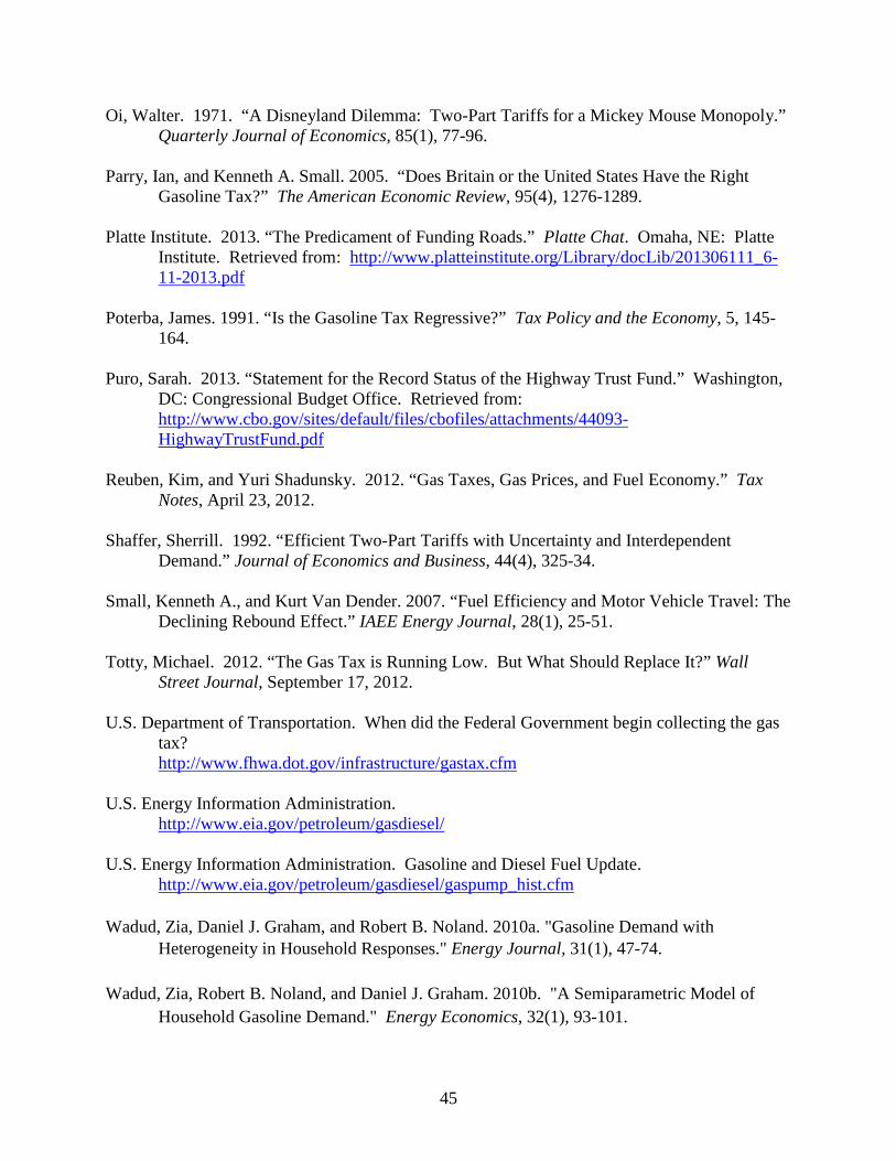
45
Oi, Walter. 1971. “A Disneyland Dilemma: Two-Part Tariffs for a Mickey Mouse Monopoly.” Quarterly Journal of Economics, 85(1), 77-96.
Parry, Ian, and Kenneth A. Small. 2005. “Does Britain or the United States Have the Right
Gasoline Tax?” The American Economic Review, 95(4), 1276-1289. Platte Institute. 2013. “The Predicament of Funding Roads.” Platte Chat. Omaha, NE: Platte
Institute. Retrieved from: http://www.platteinstitute.org/Library/docLib/201306111_6-11-2013.pdf
Poterba, James. 1991. “Is the Gasoline Tax Regressive?” Tax Policy and the Economy, 5, 145-
164. Puro, Sarah. 2013. “Statement for the Record Status of the Highway Trust Fund.” Washington,
DC: Congressional Budget Office. Retrieved from: http://www.cbo.gov/sites/default/files/cbofiles/attachments/44093-HighwayTrustFund.pdf
Reuben, Kim, and Yuri Shadunsky. 2012. “Gas Taxes, Gas Prices, and Fuel Economy.” Tax
Notes, April 23, 2012. Shaffer, Sherrill. 1992. “Efficient Two-Part Tariffs with Uncertainty and Interdependent
Demand.” Journal of Economics and Business, 44(4), 325-34. Small, Kenneth A., and Kurt Van Dender. 2007. “Fuel Efficiency and Motor Vehicle Travel: The
Declining Rebound Effect.” IAEE Energy Journal, 28(1), 25-51. Totty, Michael. 2012. “The Gas Tax is Running Low. But What Should Replace It?” Wall
Street Journal, September 17, 2012. U.S. Department of Transportation. When did the Federal Government begin collecting the gas
tax? http://www.fhwa.dot.gov/infrastructure/gastax.cfm
U.S. Energy Information Administration.
http://www.eia.gov/petroleum/gasdiesel/ U.S. Energy Information Administration. Gasoline and Diesel Fuel Update.
http://www.eia.gov/petroleum/gasdiesel/gaspump_hist.cfm Wadud, Zia, Daniel J. Graham, and Robert B. Noland. 2010a. "Gasoline Demand with
Heterogeneity in Household Responses." Energy Journal, 31(1), 47-74. Wadud, Zia, Robert B. Noland, and Daniel J. Graham. 2010b. "A Semiparametric Model of
Household Gasoline Demand." Energy Economics, 32(1), 93-101.

46
Appendix A 50 State Review of Title and Registration Fees TITLE AND REGISTRATION FEES
State AAA Links
Automobile Motorcycle Duplicates Notes
Title Fee Registra-tion Fee Title Fee Registra-tion Fee
Plate Fee Registra-tion Fee
Driver’s License Fee
Title Fee Special Plates
Alabama $18.00 $23.00 + issuance fee (may differ by county)
$18.00 $15.00 $26.19 n/a $18.50 $15.00 $50.00
Alaska $15.00 $100.00 – once every 2 years
15 $60.00 – once every 2 years
$5.00 $2.00 $15.00 $15.00 $30.00
Arizona $4.00 $8.00; ($8.25 in Metro Phoenix and Tucson) + $1.50 air quality research fee + vehicle license tax (assessed value of 60% of the MSRP - reduced by 16.25% each year)
$4.00 $9.00 $5.00 $1.00 $12.00 $4.00 $25.00
Arkansas $5.00 By weight. * $5.00 $3.00 for 0-250cc; $7.00 for 251cc+
$4.00 $1.00 $10.00 $5.00 $5.00 – $25.00
* $17.00 for cars under 3,000 lbs.; $25.00 for cars between 3,001 and 4,500 lbs.; $30.00 for cars greater than 4,500 lbs.
California $18.00 $46.00 * $18.00 $46.00 * $19.00 $18.00 $25.00 $18.00 $10.00 – $90.00 depending on type
*Plus additional fees of based on the type of vehicle, license plate type, and the owner’s county of residence and driving record.

47
Colorado $9.05 Based upon the year, weight, taxable value and month of registration.
$9.05 Based upon the year, weight, taxable value and month of registration.
Varies $2.20 $7.50 for the 1st; $14.00 for 2 or more
$8.50 Varies Additional fees based on the type of vehicle, license plate type, and the owner's county of residence and driving record.
Connecticut $25.00 $80.00 (2yrs. $40 for 1 yr.) but varies according to vehicle
$25.00 $42 (2yrs.) $5.00 $20.00 $30.00 $25.00 $50.00 – $139.00 + plate fee
Delaware If no lien: $25.00; With lien: $35.00
1-5 yrs: $40.00/yr. If no lien: $25.00; With lien: $35.00
$15.00/yr $6.00 plain plate; $10.00 special plate
$2.00 for card; $1.00 for sticker
$10.00 $25.00 $10.00 – $50.00
District of Columbia $26.00 Below 3,500 lbs: $72.00; 3,500 or above: $115.00 – $155.00
$26.00 $52.00 $10.00 $20.00 $20.00 $26.00 $100.00
Florida $77.25 - original title new $85.25 - original title used
Initial registration: $225.00 plus annual base registration. *
$77.25 $41.15 $28.00 $5.00 $25.00 $75.25 $15.00 – $25.00
* Vehicle under 2,500 lbs: $46.15; Vehicle between 2,500 – 3,499: $57.15; Vehicle 3,500 or more: $70.65.
Georgia $18.00 $20.00 $18.00 $20.00 $8.00 $1.00 $5.00 $8.00 $25.00

48
Hawaii n/a $45.00 for all motor vehicles plus an applicable weight tax. *
n/a $45.00 for all motor vehicles plus an applicable weight tax. *
$5.00 Maui County: $6.00; all other counties: $5.00
Hawaii County and Maui County: $6.00; all other counties: $5.00.
n/a $25.00 * $25.00 $0.0175 per pound for every vehicle up to 4,000 pounds net weight; $0.02 per pound for every vehicle between 4,000 and 7,000 pounds; $0.0225 per pound for every vehicle between 7,000 and 10,000 pounds; and $300 flat rate for every vehicle over 10,000 pounds. The various counties have varied rate fees as well: Honolulu City and County – $0.04 per pound; Maui County – $0.0125 per pound; Hawaii County – $0.0075 per pound; Kauai County – $0.0125 times vehicle weight plus $0.0075.
Idaho $14.00 $24.00 – $48.00; depends on vehicle age and county of residence
$14.00 $15.00 $3.00 $5.00 plus $2.00 each for stickers
$15.00 $14.00 $25.00 – $60.00 initial fee; $15.00 – $40.00 renewal
Illinois $95.00 $99.00 $95.00 $39.00 $26.00 (one); $29.00 (two)
$3.00 (cards); $20.00 (stickers)
$5.00 $95.00 $37.00 – $146.00
Indiana $15.00 $21.05 $15.00 $26.05 $10.00 $6.00 $10.00 $9.00 Varies

49
Iowa $25.00 Vehicle registration fees for vehicles up to 11 years old are $0.40 per 100 lbs. plus a percentage of the vehicle’s value as decided by the Dept. of Motor Vehicles. *
$25.00 5 years old or newer: $20.00; more than 5 years old: $10.00
$5.00 $3.00 $3.00** $25.00 $25.00 * For vehicles up to 7 years old, 1% of the list price; for vehicles 8-9 years old, 0.75% of the list price; for vehicles 10-11 years old, 0.5% of the list price. For vehicles more than 12 years old, the total registration fee is $50.00.
** Effective July 1, 2013, the driver’s license replacement fee increases to $10.00.
Kansas $10.00 $35.00 – $45.00 depending on weight
$10.00 $25.00 $3.00 $1.00 $8.00 $10.00 $46.00
Kentucky $10.00 $21.00 $10.00 $18.50 $9.00 $3.00 $12.00 $12.00 $25.00
Louisiana $18.50 Based on the selling price of the vehicle. *
$18.50 $12.00 $10.00 $12.00 $5.00 $18.50 Varies * The current rate is .1% of the value of the vehicle per year, with a minimum base of $10,000. The license plates are sold in 2-year increments, therefore the minimum price is $20.00. An $8.00 handling fee added to all transactions. A Parish fee not to exceed $3.00 is asked in certain Parishes.
Maine $33.00 $35.00 $33.00 $21.00 $5.00 Card: $2.00; Stickers: $0.50 each
$5.00 $33.00 $25.00
Maryland $100.00 By weight. * $100.00 $104.00 $20.00 $5.00 $20.00 $20.00 $15.00 – $50.00** plus additional annual fee
* $135.00 for vehicles 3,700 lbs. or less; $187.00 for
** $15.00 (non-logo); $20.00 (bay or agricultural);

50
when applicable
vehicles over 3,700 lbs. $51.00 for historic motor vehicles.
$25.00 (logo); $50.00 (vanity).
Massachusetts $75.00 $50 biannually $75.00 $20 annually
$10.00 per plate
$25.00 $25.00 $25.00 $45.00 – $100..00
Michigan $15+6% use tax
If vehicle model is earlier than 1983, then fee depends on weight. If vehicle model is 1983 or later, the fee depends on the list price of the vehicle.
$15.00 $23.00 $5.00 n/a $9.00 n/a $30.00 – $35.00
Minnesota $7.25+$6.50 title transfer fee
Registration tax system for passenger class vehicles. *
$7.25 $10.00 $8.50 $8.50 (card) $9.00 (stickers)
$13.50 $9.00 $100.00 * Tax is determined in part upon the base value of the vehicle as provided by the manufacturer when the vehicle was new, and the age of the vehicle.
Mississippi $9.00 $14.00 * $9.00 $14.00 * $10.00 $2.50 $5.00 $4.00 for motor vehicles
$31.00 + regular cost of tags
* Registration fees in addition to privilege and ad valorem taxes, and possibly sales and use taxes, depending on the county, type and value of the vehicle. Contact your local county Tax Collector for more information.

51
Missouri $8.50 Registration fee based on horsepower. *
$8.50 Registration fee based on horsepower. *
n/a $12.00 Driver’s License: $10.00 for 3 years, $12.50 for 6 years; Commercial Driver’s License: $22.50 for 3 years, $25.00 for 6 years
$8.50 $15.00 * Less than 12: $18.25; 12 and less than 24: $21.25; 24 and less than 36: $24.25; 36 and less than 48: $33.25; 48 and less than 60: $39.25; 60 and less than 72: $45.25; 72 and higher: $51.25.
Montana $12.00 Under 4 yrs. old $217.00; 5 – 10 yrs. old $87.00; 11+ yrs. old $28.00
$10-$12 depending on weight
$53.25 $5.00 $5.00 $10.00 n/a $25.00
Nebraska $10.00 $15.00 + Varies, depending on make and model of vehicle and county of residence
$10.00 $15.00 + Varies, depending on make and model of vehicle and county of residence
$14.60 $6.50 $13.50 $14.00 $30.00 – $70.00
Motor Vehicle Tax is assessed on a vehicle at the time of initial registration and annually thereafter until the vehicle reaches 14 years of age or more. It is based upon the MSRP (Manufacturer's Suggested Retail Price) of the vehicle. The MSRP on a vehicle is set by the manufacturer and can never be changed. Once the MSRP of the vehicle is established, a Base Tax set in Nebraska motor vehicle statutes is assigned to that specific MSRP range and motor vehicle tax is then assessed.
Motor Vehicle Fee is based upon the value, weight and use of the vehicle and is adjusted as the vehicle ages.

52
Nevada $28.25 By number of cars * $28.25 $33.00 + $6.00 for motorcycle safety course
$5.50 $5.00 $17.00 $20.00 $36.00 for new; $20.00 renewal
* $33.00 each for the first 4 cars; $16.50 for 5-6 cars; $12.00 for 7-8 cars; and $8.00 for 9 or more cars.
New Hampshire $25.00 * By weight $25.00 $16.00 $4.00 per plate
$15.00 $10.00 $25.00 n/a * 0-3000 lbs. $31.20, 3001-5000 lbs. $43.20, 5001-8000 lbs. $55.20, 8001-73,280 lbs. $ .96 per hundred lbs. gross weight
New Jersey $60.00 without lien
$35.50 – $84.00, based on age and weight of vehicle
$60.00 without lien
$65.00 $6.00 – $11.00
$5.00 $11.00 $60.00 $15.00 – $50.00 for new; $0.00 – $10.00 for renewal
New Mexico $3.00 $27.00 – $62.00 (1 yr) and $54.00 – $124.00 (2 yr)
$3.00 $15.00 (1 year) $30.00 (2 year)
$9.50 $3.50 $18.00 $15.00 $3.00 – $40.00
New York $50.00 plus $5.00 security interest fee
Varies based on weight. *
$50.00 plus $5.00 security interest fee
$80 (one source says $14)
$15.50 single; $28.00 pair
$3.00 $17.00 $20.00 $60.00 plus $31.25 / year
* For residents of the 12 county Metropolitan Commuter Transportation District (MCTD), a supplemental fee of $50 for two years ($25 per year) is in addition to other registration fees. Additional Vehicle Use taxes of approx $15/yr.
Registration fee for two years: $26 to $34 - Less than 2,150 lbs. $35.50 to $43.50 for 2,151 lbs. - 2,750 lbs. $45.50 to $53.50 for 2,751 lbs. - 3,350lbs. $55 to $66.50 for 3,351 lbs. - 3,950 lbs. $69 to $81 for 3,951 lbs. - 4,550 lbs. $83.50 to $95.50 for 4,551 lbs. - 5,150lbs. $98 to $110 for 5,151 lbs. -

53
5,750 lbs. $112.50 to $139 for 5,751 lbs. - 6,950 lbs. $140 for 6,951 lbs. and up +Additional fees which vary by county
North Carolina $40.00 $28.00 $40.00 $18.00 $15.00 $15.00 $10.00 $15.00 $30.00
North Dakota $5.00 $49.00 – $274.00 * $5.00 $15.00 – $25.00
$5.00 Not to exceed $5.00
$8.00 if lost, mutilated or destroyed; $3.00 for a name or address or erroneous information change
$5.00 $25.00 * Annual fee varies based on weight and 1st year of registration.
Ohio $15.00 + $1.50 to notarize signatures
$34.50 $15.00 + $1.50 to notarize signatures
$28.50 base fee, $4.00 motorcycle fee and county fees
$10.50 (one plate) $11.75 (two plates)
$4.50 $24.50 $15.00 $50.00 plus registration fee
Registration fees do not include permissive (local) taxes which vary based on the taxing district of the customer. Permissive tax cannot exceed $20.00 per vehicle and may be prorated, by law, by 50% if registering for less than 6 months.

54
Oklahoma $11.00 By year. All fees include an additional $5.75 in other fees. *
$11.00 $94 - $24 based on # of years registered
$9.00 $9.00 $10.00 $11.00 Ranges from $5.00 – $42.00, plus regular registration fees
* $91.00 for the 1st – 4th years; $81.00 for the 5th – 8th years; $61.00 for the 9th – 12th years; $41.00 for the 13th – 16th years; $21.00 for 17+ years.
Oregon $77.00 $86.00 – 2 year; $172.00 – 4 year
$77.00 $48.00 – 2 years; $96.00 – 4 years 16
$22.00 for 1; $34.00 for 2
$5.00 $26.50 $77.00 Same as plate fee + surcharge
Pennsylvania $22.50 $36.00 $22.50 $18.00 $7.50 $1.50 at original registration, transfer, or renewal; $4.50 at any other time
$13.50 ($18.50 for Class M license)
$22.50 $20.00 – $35.00
Rhode Island $51.50 Based on vehicle weight + $1.50
$51.50 Prorated by date + $1.50
$31.50 $18.50 $26.50 $51.50 $67.50
South Carolina $15.00 Depending on age * $15.00 $10.00 n/a $1.00 $10.00 $15.00 Varies * For persons 65 years or older or handicapped, the fee is $20.00; if age 64, the fee is $22.00; if under age 64, then $24.00.
South Dakota $5.00 $30.00 – $92.50 depending on vehicle’s age and weight
$5.00 $8.40 – $14.50, depending on motorcycle’s age and engine capacity
$10.00 n/a $10.00 $10.00 $25.00/yr.
Tennessee $13.00 $24.00 $13.00 $11.75 $10.00 $3.50 $8.00 for initial duplicate; $12.00 for every subsequent one thereafter
$5.50 $35.00

55
Texas $13 + 6.25% sales tax on purchase price or presumptive value whichever is higher
For vehicles under 6,000 lbs. $50.75 + local and county fees*
$13 + 6.25% sales tax on purchase price or presumptive value (plus additional county fees)
$30.00 plus local and county fees
$9.00 $3.00 $11.00 $2.00 $30.00 – $795.00
* 6.1k lbs – 10k lbs: $54.00 (plus additional county fees)
Utah $6.00 $43 vehicles </= 12k lbs. $69.50 vehicles 12k – 14k lbs. + $19.50 every 2k lbs over 14k lbs.
$6.00 $44.50 $5.00 $4.00 $18.00 $6.00 Up to $55.00
Vermont $33.00 $77 (gas) $27 (diesel) $122 (other) (1 yr.) and $129 (gas) $50 (diesel) $225 (other) (2 yrs.)
$33.00 $44.00 $10.00 per plate
$15.00 $15.00 $33.00 $45.00
Virginia $10.00 $40.75 - less than 4,000 lbs. $45.75 - more than 4,000 lbs.
$10.00 $28.75 $10.00 $2.00 $10.00 $10.00 $10.00/year
Washington $15.50 $30.00 plus $3.75 state fee, variable weight fee, and local fees
$15.50 $30.00 plus $10 weight fee and $3.75 state fee
$27.75 auto $7.75 motorcycle
$5.00 $20.00 $19.00 for motor vehicles
$40.00 initial and $30.00 renewal
Please visit the Washington Department of Licensing for more information on vehicle and drivers licensing fees.
West Virginia $10.00 For vehicles weighing under 8,000 lbs.: $30.00
$10.00 $16.00 $5.50 $5.00 $5.00 n/a Varies
Wisconsin $69.50 $75.00 $69.50 $23.00 (biennial fee)
$2.00 – $6.00
$2.00 $14.00 $20.00 $5.00 – $75.00
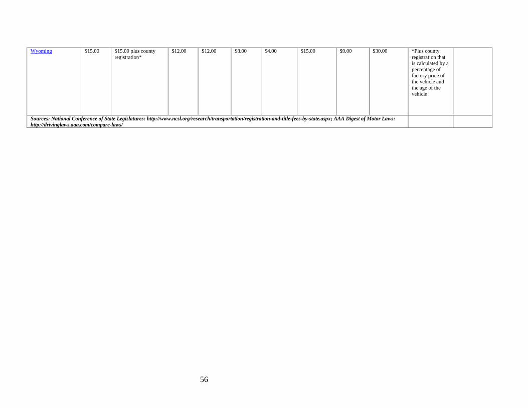
56
Wyoming $15.00 $15.00 plus county registration*
$12.00 $12.00 $8.00 $4.00 $15.00 $9.00 $30.00 *Plus county registration that is calculated by a percentage of factory price of the vehicle and the age of the vehicle
Sources: National Conference of State Legislatures: http://www.ncsl.org/research/transportation/registration-and-title-fees-by-state.aspx; AAA Digest of Motor Laws: http://drivinglaws.aaa.com/compare-laws/

57
Appendix B Theory 1.1 Model
Consider the production of transportation services using two inputs: automobile capital x and
gasoline g. The production function is given by,
𝑞 = 𝐴𝑔𝛼𝑥𝛽 (1)
where the exponents 𝛼,𝛽 are strictly within the unit interval [0,1]. The sum of α and β reflects
the economy of scale in the production of transportation services embodied in the technology of
(1). We assume that +𝛽 < 1 , indicating decreasing returns to scale and strict concavity of the
production function.
The cost C of producing transportation services is given by the sum of expenditures on
gasoline and automobile capital,
𝐶 = 𝑟𝑔𝑔 + 𝑟𝑥𝑥 (2)
where 𝑟𝑔, 𝑟𝑥 are the exogenous input prices.
We can either proceed to derive the implications of the constrained output maximization
problem or its dual, the constrained cost minimization problem. In what follows, we focus on
the dual problem as it is the more natural way to think of situation in our context.
Minimization of C subject to a given level of output 𝑞0 proceeds by forming the usual
Lagrangian function L, used in constrained optimization, with the associated multiplier 𝜆.
𝐿 = 𝑟𝑔𝑔 + 𝑟𝑥𝑥 + 𝜆[𝑞0 − 𝐴𝑔𝛼𝑥𝛽] (3)
Differentiation of (3) with respect to g, x, and 𝜆 yields the first order conditions:
𝜕𝐿𝜕𝑔
= 𝑟𝑔 + 𝜆�−𝛼𝐴𝑔𝛼−1𝑥𝛽� = 0 (4)
𝜕𝐿𝜕𝑥
= 𝑟𝑥 + 𝜆�−𝛽𝐴𝑔𝛼𝑥𝛽−1� = 0 (5)
𝜕𝐿𝜕𝜆
= 𝑞 − 𝐴𝑔𝛼𝑥𝛽 = 0 (6)

58
Second order conditions must also be met to assure a minimum of cost, rather than a maximum,
but we can be assured that those conditions will hold if the production function is strictly quasi-
concave, which it is given our assumption regarding the production technology.
Equations (4) and (5) together yield the relationship known as the rate of technical
substitution (RTS) between g and x. The RTS is the ratio of the marginal products of the two
inputs and indicates that rate at which one input can be substituted for the other input in the
production of transportation services while maintaining the same output. When graphed in input
space, the RTS traces out the expansion path.
𝑥𝑔
= �𝑟𝑔𝑟𝑥� �𝛽
𝛼� (7)
This relationship indicates that the ratio of inputs x and g is constant as output is scaled up, with
the ratio depending on two factors: the relative prices of the inputs and the production
technology, captured by the production function coefficients 𝛼,𝛽. Solving this relationship for x
yields the expression,
𝑥 = 𝑔 �𝑟𝑔𝑟𝑥� �𝛽
𝛼� (8)
Hence, the relationship between x and g is linear as output is expanded or cost is reduced. The
slope of that linear relationship depends on the ratio of input prices and the production
technology.
Inserting equation (8) into (4) and solving for g gives the input demand expression for
gasoline,
𝑔 = 𝐵𝑔 �𝑟𝑥𝑟𝑔�
𝛽𝛼+𝛽
(9),

59
where 𝐵𝑔 = �𝑞1
𝛼+𝛽𝐴−1
𝛼+𝛽(𝛼𝛽
)𝛽
𝛼+𝛽�. Hence, the demand for gasoline is inversely related to its own
price, 𝑟𝑔, but it is directly related to the price of automobile capital, 𝑟𝑥.
Similarly, we can solve for the input demand function for x,
𝑥 = 𝐵𝑥 �𝑟𝑔𝑟𝑥�
𝛼𝛼+𝛽 (10)
where 𝐵𝑥 = �𝑞1
𝛼+𝛽𝐴−1
𝛼+𝛽(𝛼𝛽
)−𝛼𝛼+𝛽�. Again, the demand for automobile capital is inversely related
to its own price, but is directly related to the price of gasoline.
Using the two input demand functions, we can derive the cost function by substituting
expressions (9) and (10) into (2), thereby deriving cost C as a function of output q:
𝐶 = 𝑞1𝛼+𝛽� [(𝛼 + 𝛽)( 𝑟𝑔𝛼𝑟𝑥
𝛽
𝐴𝛼𝛼𝛽𝛽)1𝛼+𝛽� ] (11)
This expression can be simplified to,
𝐶 = 𝑐𝑞1𝛼+𝛽� (12)
where c is the constant, 𝑐 = (𝛼 + 𝛽)( 𝑟𝑔𝛼𝑟𝑥𝛽
𝐴𝛼𝛼𝛽𝛽)1𝛼+𝛽� . Hence, the cost of transportation services
rises with output. The nature of that increasing relationship depends on the production function
parameters, however. The cost function is convex if 𝛼 + 𝛽 < 1, linear if 𝛼 + 𝛽 = 1, and
concave if 𝛼 + 𝛽 > 1.
1.2 Effect of Various Taxes (comparative static analysis)
a. Ad valorem tax applied to gasoline: 𝜏𝑔
i. Inclusion of an ad valorem tax on gasoline alters the input demand
functions as follows:

60
1. 𝑔′ = 𝐵𝑔 �𝑟𝑥
(1+𝜏𝑔)𝑟𝑔�
𝛽𝛼+𝛽
(9’),
2. 𝑥′ = 𝐵𝑥 �(1+𝜏𝑔)𝑟𝑔
𝑟𝑥�
𝛼𝛼+𝛽 (10’)
3. Clearly, the tax reduces the demand for gasoline and increases the
demand for automobile capital.
ii. The cost function is also affected by the inclusion of the tax …
b. Unit tax applied to gasoline: 𝑡𝑔
i. Inclusion of a unit tax on gasoline also alters the demand functions, as
follows
1. 𝑔′ = 𝐵𝑔 �𝑟𝑥
𝜏𝑔+𝑟𝑔�
𝛽𝛼+𝛽
(9’’),
2. 𝑥′ = 𝐵𝑥 �𝜏𝑔+𝑟𝑔𝑟𝑥
�𝛼
𝛼+𝛽 (10’’)
3. Once again, the tax reduces the demand for gasoline and increases
the demand for automobile capital.
4. But, the effects of the unit tax and the ad valorem tax differ.
ii. If we set (9’’) = (9’) we can derive the relationship between ad valorem
and unit taxes that will have the same impact on gasoline and automobile
capital demand:
1. 𝑡𝑔 = 𝑟𝑔𝜏𝑔, or 𝜏𝑔 = 𝑡𝑔𝑟𝑔� .
2. Hence, if we wish to replace the current unit tax with an ad
valorem tax with the same impact on gasoline demand, the ad

61
valorem tax should be set equal to the ratio of the unit tax divided
by the price of gasoline.
3. The main advantage of an ad valorem tax rate is that as the price of
gasoline rises over time, revenues generated by the tax rise as long
as the price elasticity of demand is less than one (in absolute
value). With a unit tax, as the price of gasoline rises the quantity
demanded is reduced and revenues generated by the tax decline.
4. Note: If both an ad valorem gasoline tax and a sales tax are
applied, the sales tax should be applied to the price of gasoline
exclusive of the gasoline excise tax.
c. Two-part tariff: 𝑇, 𝜏𝑔
i. A flat rate tax T plus an ad valorem gas tax are included in the model:
ii. Cost of producing transportation service is modified to become:
1. 𝐶′ = 𝑇 + (1 + 𝜏𝑔)𝑟𝑔𝑔 + 𝑟𝑥𝑥