relative cohort size and unemployment in the united states
TRANSCRIPT

Relative Cohort Size and Unemployment in
the United States
Carsten Ochsen�
September 21, 2012
Abstract
Since the early 1970s it was argued in di¤erent studies that shifts
from relative smaller to larger age cohorts of the labor force lower the
unemployment rate (cohort crowding hypothesis). However, Robert
Shimer (2001) provoked a debate with his controversial result that the
overall unemployment rate tends to be lower when many young people
supply labor. In contrast to other studies, he uses regional (state level)
data. In this study I apply di¤erent regional data sets for the USA
(including Robert Shimers original data) to analyze how aging a¤ects
unemployment in a framework that considers spatial interactions. At
the state level, I can neither con�rm the �ndings of Robert Shimer nor
the cohort crowding hypothesis. Using county level data, however, I
�nd local e¤ects that are compatible with the cohort crowding hy-
pothesis but also with speci�c assumptions about the heterogeneity of
older and younger workers that are to the advantage of older workers.
Keywords: Regional Unemployment, Spatial Interactions, Aging, Panel
Data, Spatial Model
JEL classi�cation: J60, R12, J10, C23
�University of Applied Labour Studies, University of Rostock, and Max Planck Insti-tute for Demographic Research; e-mail: [email protected]. I am gateful toChris Foote, Ron Lee, Thomas Lindh, Robert Shimer, and participants of the 4th WorldConference of the Spatial Econometrics Association in Chicago and the 65th EuropeanMeeting of the Econometric Society in Oslo.
1

1 Introduction
The literature on the e¤ects on unemployment of di¤erences in population
age cohorts originated in a study by George Perry (1970), who, along with
Richard Easterlin, pioneered the hypothesis of cohort crowding. Using this
hypothesis, a number of authors have argued that an increase in the per-
centage of youth in the working-age population raises the unemployment
rate since the level of the unemployment rate is generally higher for younger
workers.1 All these studies used macroeconomic data.
A di¤erent approach from that of the cohort crowding hypothesis is found
in Robert Shimers (2001) article, who used regional data for 1973-1996 to
estimate the impact on overall unemployment rate of changes in the percent-
age of youth aged 16-24 in the population. In his analysis of US local labor
markets, Robert Shimer found that the overall unemployment rate tends to
be lower when many young people supply labor and argued that a high pro-
portion of young workers incents �rms to create new jobs because younger
workers undertake more search activities, which reduce the �rms�recruitment
costs.
However, Chris Foote (2007) extended the sample period 1973-2005 and
found no signi�cant relationship between the unemployment rate and the
proportion of youth in the population. Carsten Ochsen and Pascal Hetze
(2006) discussed two other problems: First, many talented young people are
still pursuing their education at these ages, so the level of formal education
of those in the labor market is lower in this cohort than in older age groups.
Second, Shimer used percentage of overall population and did not control for
the percentage of di¤erent age groups who were in the labor market. The
correlation coe¢ cient between the labor market participation rate for the 16-
64 age group and 16-24 age group is -0.2. One of the important reasons for
this non-conforming trend in labor market participation is that the average
duration of education for young people has steadily increased over the last
decades.
A further issue is the consideration of spatial correlation. Carsten Ochsen
1See, for example, Bloom et al. (1987), Flaim (1979, 1990), Gordon (1982), Gracia-Diez (1989), and Korenman and Neumark (2000).
2

(2009) used regional (county level) panel data for Germany in a spatial and
time dynamic model. Using the age group 16-39 as the de�nition of the
young, regional unemployment declines the more younger worker are in the
surrounding regions. Ochsen argues that this is because of the higher mobility
(in terms of commuting) of younger workers. At the local level, neither the
cohort crowding nor the Shimer e¤ect can be con�rmed. However, although
the results are di¤erent, overall they point in the same direction as Robert
Shimers results.2 The cohort crowding e¤ects can be overlaid by age-related
changes in matching e¢ ciency, job creation, and job destruction.
The present study contributes to the literature by using di¤erent regional
data sets (at the state level and the county level) for the US and a new
estimator to analyze the e¤ects of smaller cohorts on the labor market, in
particular, the issues of spatially dependent local labor markets. In addition,
I consider di¤erent cut o¤s for the delineation between young and old. Fi-
nally, I present a theoretical model that provides an explanation for the e¤ects
found. I argue that the two age groups di¤er in their employment-related
attributes (e.g., productivity, matching e¢ ciency, and labor turnover), apart
from cohort size.
The analysis I o¤er, undertaken to identify the demographic e¤ects on
unemployment, provides theoretical implications and empirical �ndings for
the US labor market. Using di¤erent regional data and spatial and time
dynamic econometric models, I examine empirically the consequences of an
aging working-age population for the local labor markets. According to the
estimates using county level data, ongoing aging in the local labor market
causes a fall in local unemployment. In addition, aging in the surrounding
areas has a positive e¤ect on unemployment in the local district. My in-
terpretation is that �rms prefer older workers, but this age group also has
less spatial mobility (in terms of commuting), which declines the matching
e¢ ciency and reduces job creation. Using state level data, I �nd neither the
cohort crowding e¤ect nor the Shimer e¤ect.
2Using Shimer�s data, Foote (2007) also showed that the consideration of spatial corre-lation at the state level reveals that the youth share e¤ect is no longer signi�cant. However,he considers "only" the Driscoll and Kraay standard errors, which is not su¢ cient to con-sider spatial correlation.
3
2 Theoretical Model
In most cases, the literature that has dealt with age and employment or
matching is related to speci�c issues. Christopher Pissarides and Jonathan
Wadsworth (1994) and Simon Burgess (1993) found evidence for Great Britain
that the rates of job separation are higher for young workers because they
are more likely to conduct job searches while they are employed.3 Hence, as
Melvyn Coles and Eric Smith (1996) argued in their study on England and
Wales, matching may decrease with an older working population. Job sepa-
rations and low hiring rates for older workers could also be the result of imag-
ined or actual di¤erences in productivity (Haltiwanger et al. 1999, Daniel
and Heywood 2007); productivity may increase with age if job experience is
important (Autor et al., 2003) and decline if human capital depreciates over
a lifetime, as it may in a dynamic technological environment or when manual
abilities are central to productivity (Bartel and Sicherman 1993, Hellerstein
et al., 1999, Börsch-Supan 2003).
The willingness to create new jobs may also change because of changes in
mobility in an aging labor force. According to Herbert Brücker and Parvati
Trübswetter (2007) and Jennifer Hunt (2000), regional mobility decreases as
age increases for both high- and low-skilled workers as well as for employed
and unemployed people. The causes for this decreasing mobility after a
certain point in life are, for example, housing tenure, partner�s economic
status, and childcare.4
Another important issue in the context of mobility is that of spatial de-
pendencies of the regional labor markets. The performance of a local labor
market depends, among other things, on the characteristics of the regional
labor markets in the surrounding area. For example, job creation can be
a¤ected by the age structure of the labor force in the neighbor districts since
regional mobility di¤ers between age groups. Although it seems obvious that
regional mobility plays an important role at the regional level, only a few
studies have considered spatial interactions in the labor market. René Fahr
and Uwe Sunde (2005) used data at the regional level for West Germany to
3Davis et al. (1996) found evidence for the US that job �ows are higher for youngworkers.
4See, for example, Lindley et al. (2002) for a detailed discussion of these causes.
4

estimate a matching function. Their results indicate that matching is pos-
itively related to the percentage of young participants in the labor market.
Using regional data, Michael Burda and Stefan Pro�t (1996) also considered
the spatial dimension in the matching function for the Czech Republic, as
Barbara Petrongolo and Etienne Wasmer (1999) did for France and the UK,
Simon Burgess and Stefan Pro�t (2001) for the UK, and Reinhard Hujer et
al. (2009) for Germany. These studies found signi�cant spatial interactions
in regional search activities or unemployment rates.
With respect to aging of the labor force, I follow Carsten Ochsen (2009)
and extend the framework of search and equilibrium unemployment by dis-
tinguishing between younger and older workers and between the age-related
e¤ects.5 By considering age-sensitive di¤erences in separation risks, mobil-
ity, labor productivity, and wages, I di¤erentiate between younger and older
workers who may generate di¤erent levels of surplus for �rms if they �ll a
vacancy.
To retain simplicity, I treat on-the-job searches di¤erently from the way
they are treated in the standard framework (see Pissarides, 2000) in that I
do not consider the two usual reservation productivity parameters that allow
di¤erentiation between productivity-related job destruction and on-the-job
search.6 In general, this approach helps to explain why employed people
decide in favor of on-the-job search. The focus in this paper, however, is on
the consequences of spatial search activities on matching, job creation and
job destruction.
I consider two types of agents: workers and �rms. All agents are risk
neutral and discount the future at rate r. The labor force is divided into
two age groups� younger workers y and the older workers o� with shares of
p and (1� p), respectively. Workers are either employed or unemployed, andif they are unemployed, I assume that they seek a new job. The average
rate of unemployment u in a continuum of workers, normalized to 1, consists5We analyze the e¤ects of aging of the labor force but ignore the e¤ects of a decline
in population because most empirical studies �nd constant returns to scale of matchingfunctions. Petrongolo and Pissarides (2001) provided an overview of the related literature.Therefore, the pure population size has no e¤ect on matching and search equilibrium inthe labor market.
6Up to half of all new employment relationships result from a job-to-job transition.See, for example, Blanchard and Diamond (1989) and Fallick and Fleischman (2004).
5
of the age-speci�c rates weighted at the relevant labor force share: u =
puy + (1� p)uo.New employment relationships are created through a matching technology
that forms the number of matches from the number of unemployed workers,
the number of on-the-job searchers, and the number of vacancies. That is, the
standard matching technology is enlarged by a rate e, which is the percentage
of the employed who search on-the-job for new employment. Hence, I have a
search rate of � = u+ e, which is the sum of unemployed and employed job
seekers divided by the labor force, with e � 1� u.At the regional level, it is obvious that people apply for jobs in surround-
ing regions and workers commute between their home region and their work-
place region. In addition, the bulk of these commuting dependencies apply
to regions that are adjacent. Thus, I refer to commuting and inter-regional
searches as mobility. However, this de�nition of mobility does not include
moves from one region to another. To maintain the model�s simplicity, I
consider job seekers and vacancies only from the local region l and regions
adjacent to l, which I treat as one homogenous region, n.
Equilibrium in search models usually depends on the tightness of the
labor market because it is that tightness that determines how successful a
search is likely to be. The tightness of the local labor market is given by
�l = vl=�ul + el + ~un + ~en
�= vl=
��l + ~�n
�,
and the tightness of the adjacent districts�labor market is given by
�n = vn=�un + en + ~ul + ~el
�= vn=
��n + ~�l
�,
where vl (vn) denotes the local (neighborhood) vacancy rate and � rep-resents spatial search activities. I assume that job seekers apply for jobs in
their home regions, but the number of regional mobile job applicants depends
on the age structure of the job seekers because younger workers are more mo-
bile. Hence, only a part of the older job seekers from neighbor regions apply
for jobs in the local region. I refer to �l = pl�ly +�1� pl
��lo and �
n =
6
pn�ny + (1� pn)�no as local search rates and ~�n =�pn�ny + (1� pn)�no�
�Ln
Ll
and ~�l =�pl�ly +
�1� pl
��lo�
�Ll
Lnas spatial search rates.
Workers (employed and unemployed) resident in the local region, Ll, are
normalized to 1. The rate ~�n is related to the labor force in the local labor
market, Ll, and so has the same denominator as �l. There are two di¤erences
between ~�n and �n: First, they are related to di¤erent labor force sizes�
~�n to the local labor force and �n to the labor force in the adjoining areas,
Ln. Second, the share of older job seekers is larger in their resident region,
�no > �no�. The mobility weighting factor �, with 0 � � < 1, accommodates
the limited spatial mobility of older workers. The di¤erences between ~�l and
�l are analog to those between ~�n and �n.
The age distribution of the job seekers who are available to local �rms
di¤ers from both pl and pn. The proportion of young applicants (from the
local and the surrounding area) available to �rms in the local labor market is
pl�ly
�l+~�n+ pn
�ny�l+~�n
� �pl. Hence, the age structure of the job seekers depends
on the age structure of the labor force.
To introduce a nonstandard matching technology that re�ects the age
composition of the job seekers, I consider job seekers in e¢ ciency units iden-
ti�ed by �, depending on the share of the young available to local �rms ���pl�.
The number of job seekers in e¢ ciency units ���pl�(�l + ~�n) measures the
average age-related search intensity, in addition to a quantitative e¤ect. For
example, lower search intensity, as is often assumed for older workers, should
reduce unemployment in e¢ ciency units. Therefore, I assume that �0 > 0
and �00 < 0.
Thus, I have the local matching function ml = ml(���pl�(�l + ~�n); vl)
as the local labor market �ow rate of matches (in e¢ ciency units) formed.
A local �rm with a vacancy meets a job seeker at a rate of ql(�l; �pl) �ml(�
��pl�1�l; 1), a rate that decreases with the vacancy-unemployment ratio
and increases with the share of young job seekers. Hence, when @ql(�l;�pl)
@�l< 0
a low vacancy/job seeker ratio increases the chances of �lling a vacancy, but
only at a given e¢ ciency level. The derivation @ql(�l;�pl)@�pl
> 0 means that, the
larger the percentage of young job seekers available in the labor force, the
easier it is for �rms to �nd a job seeker at a given number of job seekers and
vacancies.
7
Correspondingly, a job seeker �nds new employment in the local region
at rate �lql(�l; �pl)�ml(���pl�; �l), which is identical for both age groups be-
cause vacancies do not di¤erentiate between younger and older candidates.
A higher percentage of younger job seekers implies e¢ cient matching and,
therefore, a higher rate of job search success,@(�lql(�l;�pl))
@�pl> 0. Hence, aging
decreases the matching e¢ ciency and both sides� �rms and job seekers�
will require more time to �nd the appropriate job (candidate). Finally, a job
seeker from the local region �nds, on average, new employment at the rate
�lql(�l; �pl) + �nqn(�n; �pn) because of his or her spatially mobile search activi-
ties. It follows, then, that the spatial correlation of unemployment rates are
positive. In addition, both the local and spatial vacancy rates are negatively
correlated with the unemployment rates.
Job-worker matches have a �nite time horizon. Separation occurs be-
cause of idiosyncratic shocks that hit all matches at the same probability
s. Age-related shocks are also possible. For example, let � o and � y denote
the rates of the added risk that the match will end based on whether the
worker is older or younger, respectively. The rates may also include di¤erent
quitting rates (labor turnover rates)� for example, because of di¤erences in
regional mobility. In addition, I allow for regional di¤erences of (age-speci�c)
separations to accommodate the large regional di¤erences in unemployment.
Finally, from the perspective of the local region, I add the probability
that a mobile worker loses his or her job in the surrounding area. The local
labor force, Ll, can be subdivided into three groups: local unemployed ul,
residents employed in the local region !l;l, and residents employed in the
neighbor region !l;n. Since Ll = 1, we have ul + !l;l + !l;n = 1.
The local unemployment rates of younger and older workers evolve ac-
cording to job creation and job destruction, with i = [y; o]:7
_uli =�sl + � li
� �1� !l;ni � uli
�+ (sn + �ni )!
l;ni (1)
��lql(�l; �pl)uli � �nqn(�n; �pn)uli.
The �rst term on the right-hand side is the age-related �ow into unem-
ployment from local employment. The second term on the right-hand side
7However, the simplifying assumption is that the spatial �ows are of equal size.
8
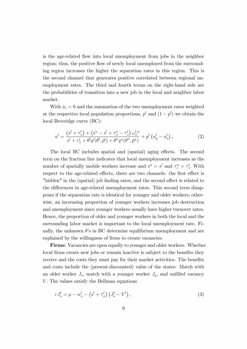
is the age-related �ow into local unemployment from jobs in the neighbor
region; thus, the positive �ow of newly local unemployed from the surround-
ing region increases the higher the separation rates in this region. This is
the second channel that generates positive correlated between regional un-
employment rates. The third and fourth terms on the right-hand side are
the probabilities of transition into a new job in the local and neighbor labor
market.
With _ui = 0 and the summation of the two unemployment rates weighted
at the respective local population proportions, pl and (1� pl) we obtain thelocal Beveridge curve (BC):
ul =
�sl + � lo
�+�sn � sl + �no � � lo
�!l;no
sl + � lo + �lql(�l; �pl) + �nqn(�n; �pn)
+ pl�uly � ulo
�. (2)
The local BC includes spatial and (spatial) aging e¤ects. The second
term on the fraction line indicates that local unemployment increases as the
number of spatially mobile workers increase and sn > sl and �ni > �li. With
respect to the age-related e¤ects, there are two channels: the �rst e¤ect is
"hidden" in the (spatial) job �nding rates, and the second e¤ect is related to
the di¤erences in age-related unemployment rates. This second term disap-
pears if the separation rate is identical for younger and older workers; other-
wise, an increasing proportion of younger workers increases job destruction
and unemployment since younger workers usually have higher turnover rates.
Hence, the proportion of older and younger workers in both the local and the
surrounding labor market is important to the local unemployment rate. Fi-
nally, the unknown ��s in BC determine equilibrium unemployment and are
explained by the willingness of �rms to create vacancies.
Firms: Vacancies are open equally to younger and older workers. Whetherlocal �rms create new jobs or remain inactive is subject to the bene�ts they
receive and the costs they must pay for their market activities. The bene�ts
and costs include the (present-discounted) value of the states: Match with
an older worker Jo, match with a younger worker Jy, and un�lled vacancy
V . The values satisfy the Bellman equations
rJ lo = �� wlo ��sl + � lo
� �J lo � V l
�, (3)
9

rJ ly = �+ � � wly ��sl + � ly
� �J ly � V l
�, (4)
rV l = � + ql(�l; �pl)�J l � V l
�. (5)
Local �rms receive revenues � from selling their output if an older worker
is employed, while they pay the wage wlo as compensation. The younger
worker produces the value �+� and earns wly. Experience and lower training
costs favor older workers, but a lower depreciation of human capital is an
argument for the higher productivity of younger workers. Hence, I do not �x
the sign of the output di¤erential, so � R 0.8 The job-worker match ends atthe probability sl + � li, in which case the value of the match is replaced by
the value of an un�lled vacancy.
The vacant job costs per unit time and changes state according to the
rate ql(�l; �pl). Hence, given that younger workers are favored, an increase in
the percentage of younger workers in the local and surrounding area increases
the number of vacancies in the local labor market. The change of state yields
net return J l � V l, where J l denotes the expected value of a �lled vacancy.Since the �rm can use two types of workers, I consider that the worker is
younger at probability �pl, and older at probability�1� �pl
�. The expected
value of �lling the local vacancy is
J l = �plJ ly +�1� �pl
�J lo. (6)
The expected value of �lling the vacancy is locally di¤erent if the age-
related values Jy and Jo have regional di¤erences and/or if �pl 6= �pn.The candidates available to local �rms are stochastically drawn from the
pool of job seekers. Firms will accept the �rst applicant for work as long
as the added costs of rejection are equal to the added gain that could be
realized by employing a superior worker. In this case, the expected value of
a vacancy is zero because waiting is worthless. This expectation holds true
if J l = =ql(�l; �pl); with eq. (6), the equation for the expected J l, we have:
8See Börsch-Supan (2003) and Hutchins (2001) on the di¢ culty of measuring individualage-related productivity.
10

1
ql(�l; �pl)=1
��plJ ly +
�1� �pl
�J lo�. (7)
the second important equation, the local job creation condition (JC).
Market tightness is the only variable parameter, and it guarantees the iden-
tity of eq. (7). Firms open more vacancies if 1=ql(�l; �pl) increases. Clearly,
easy search conditions and high pro�ts foster job creation.
E¤ects of Aging: Next, I analyze the e¤ects of a change in the agestructure and in the Appendix I provide the comparative static e¤ects. A
decline in the local share of the young reduces the average �ows in the labor
market if younger workers separate from jobs more often, while a lower to-
tal separation risk corresponds to less equilibrium unemployment. Thus, a
higher percentage of older workers reduces the labor turnover such that fewer
job-worker pairs must be matched: the BC shifts inwards. The (spatial) ef-
fect of the change in matching e¢ ciency is negative because a decline in the
local share of the young increases the average duration of the search on either
side; hence, this aging e¤ect shifts the local BC outwards. With respect to a
new equilibrium in the local BC, it follows that aging has ambiguous e¤ects.
Hence, Perry�s demographic e¤ect� that is, that a decline in unemploy-
ment is a side e¤ect of aging because uly > ulo� cannot be observed if this
e¤ect is overcompensated by an increase in unemployment in both age groups
that is due to the lower matching e¢ ciency. In addition, even if age related
separations are equal, aging increases unemployment because the BC shifts
outwards (due to a declining matching e¢ ciency). With respect to the spatial
age e¤ect, the local unemployment rate responds to a change in the spatial
share of the young in a similar way.
With respect to job creation, aging in�uences local job creation by two
means. The �rst comes from a possible di¤erence between the value of a
match with a younger and one with an older worker. If �rms value young
workers more highly than they do older workers, an aging labor force reduces
job creation and vacancies, and vice versa. The second way that an aging
labor force a¤ects local job creation comes from the e¢ ciency of matching.
As we have a negative e¤ect of aging on matching, job creation su¤ers from
11

aging. However, the total e¤ect is ambiguous. For example, when �rms favor
older workers, but the overall e¤ect of aging is still negative, the positive
e¤ect of the employment characteristics of older workers are outweighed by
the e¤ect of decreasing matching e¢ ciency. These �ndings are related to
the age structure in the local and the surrounding labor market. Hence, in
principle, the two aging e¤ects can be caused by a change in the age structure
in both regions.
Figure 1 shows equilibrium in the local vacancy-unemployment space and
illustrates the e¤ects that can arise if the age structure in�uences �ows in
the labor market and job creation. The steady state condition for unemploy-
ment is the local BC, which is convex to the origin by the properties of the
matching technology. As usual, the BC is downward sloping: unemployment
is low if the vacancy rate is high because job seekers �nd new employment
easily. The local JC, the curve that maps the job creation condition, has a
positive intercept�el + ~�n
��l and shifts when the number of local employed
job seekers or the number of spatially mobile job seekers changes. Firms
create more jobs if local unemployment is high (for a given intercept of the
JC), and the JC slopes upward.
Figure 1 about here
I found three di¤erent e¤ects: �rst, aging reduces job destruction (given
that � y > � o); second, aging reduces matching e¢ ciency; and third, aging
a¤ects productivity (positive or negative). The �rst e¤ect shifts the BC
inward, the second shifts the BC outwards and rotates the JC clockwise, and
the third e¤ect rotates the JC either clockwise or counterclockwise.
Spatial interactions of regional labor markets can cause these e¤ects on
the local labor market as well. For example, the JC rotates clockwise if the
number of mobile job searchers from the surrounding areas decreases because
this increases search costs for �rms and this, in turn, decreasing the num-
ber of vacancies as well as market tightness.9 The e¤ect of fewer mobile job
searchers on equilibrium employment is ambiguous because the reemploy-
ment probability of the local unemployed could increase, which would shift
the BC inward.9The intercept also decreases in this case.
12

3 Empirical Analysis
In this section I analyze empirically the relation between a change in the age
structure of the working-age population and the unemployment rate using
macro economic and regional data for the US. Following the cohort crowding
literature the share of the young in the working age population is positively
correlated with the overall unemployment rate. Figure 2 shows the share of
the 15-24 years old in the working age population and the �ve years smoothed
overall unemployment rate for the US. As expected, both series are positively
correlated but at a moderate level (correlation is 0.2). Overall it does not
seem that both series are "synchronized".
Figure 2 about here
Using the share of the 15-39 years old as the young the pattern changes
a little. Figure 3 shows the relation between the share of this age cohort
and the smoothed overall unemployment rate. Here, the correlation is 0.67.
Using data at the national level one can at least conclude that there is some
considerable correlation. However, using regional data allows to consider a
more di¤erentiated pattern.
Figure 3 about here
First, we start with state level data and the econometric model considered
in the 2001 article of Robert Shimer:
lnuit = � ln youngit + ci + �t + �it (8)
where lnuit is the logarithm of the overall unemployment rate in region
i and year t, ln youngit is the share of the young (share of the working-age
population who are aged 16-24) in region i and year t, ci are regional and
�t are time e¤ects, and �nt is an error term. The parameter � is positive in
Robert Shimers analysis of US state level data, which means that a larger
share of the young in state i and year t correspond to a lower unemployment
rate in this year and state. This result contradicts the cohort crowding
13

hypothesis and related to the current demographic change this means that
unemployment is positively correlated with aging. The main result in his
article is provided in table 1.
To consider that young people are likely to migrate to states with rel-
atively low unemployment rates, Robert Shimer uses lagged birth rates as
instruments. Such migration �ows can cause a spurious negative correla-
tion between low unemployment rates and high youth shares, fosters aging
in regions with high unemployment rates, and decreases market tightness
(increases unemployment) in the preferred region, given that uy > uo. How-
ever, Robert Shimer concludes that, the instrumental variable estimates do
not yield signi�cant di¤erent results, and in some cases it turns out that the
share of the young is not exogenous.
Chris Foote (2007) extends the data used in the Shimer paper by nine
years and uses the same estimation strategy. However, he does not found
a signi�cant relationship between local unemployment and the share of the
young in this region. He also considers the same instrumental variable (IV)
procedure as Robert Shimer does, but the results do not change. In addition,
Chris Foote uses corrected standard errors as suggested by John Driscoll
and Aart Kraay (1998). They provide a method that additionally to het-
eroskedasticity and autocorrelation considers spatial correlation. However,
since for each year only one average value across all regions is considered
to account for spatial correlation, this approach does not account adequate
for neighborhood correlations. Chris Foote comes to the conclusion that the
consideration of spatial correlation (by using Driscoll and Kraay standard
errors) is a further argument why the e¤ects in Robert Shimers data are in
fact not signi�cant. The main result in his article is provided in table 1.
Table 1 about here
I argue that, in principle, the local share of the young should capture
changes in the matching e¢ ciency, di¤erences in job destruction and di¤er-
ences in the value of a match with a younger or older worker that stems
from a change in age composition in the local region. To consider additional
spatial e¤ects, I enlarge the speci�cation of eq. (8). First, I will consider
spatial and time lagged e¤ects of the dependent variable, and second, and
14

this is what I am primarily interested in, I also want to capture the e¤ect of
the share of the young in the neighbor region on local unemployment.
I argue that the young in both regions are homogeneous. However, the
young in the local region do not need to be mobile to accept a job o¤er
in their home region. The young in the neighbor region, however, need to
be spatial mobile, in terms of commuting, to work in the local region. I
distinguish this from the fact that they could move to the region where they
work. Because in this case, they are living and working in the same region
(after they have moved) and I do not consider them as spatial mobile. In the
theoretical section I have argued that younger workers are more mobile than
older workers are. If this is true, I need to consider an e¤ect of the share of
the young in the neighbor region on local unemployment. Since the young in
both regions hold, on average, the same job relevant characteristics, I do not
argue that, e.g., the young in neighbor regions are more productive that the
young in the local region. In fact, this is not possible, because in my model
every share will be considered for the local region and for the neighbor region
(I am the neighbor of my neighbor).
To capture time invariant unobservables in the econometric model, a �xed
e¤ects speci�cation is considered. To account for additional unobserved time
variant e¤ects at the local level, I also considered time lagged and spatial
lagged e¤ects. In order to generate spatially lagged counterparts, I con-
structed a spatial weight matrix, W , that indicates the contiguity of regions,
and de�ned contiguity between two regions as those that share a common
border. First, the matrix has the entry 1 if two regions share the same border
and 0 otherwise. Then, I row normalize W , which ensured that all weights
were between 0 and 1 and that weighting operations can be interpreted as
an average of the neighboring values. W lnuit generates the average values
of the regions adjacent to region i. This is the spatial lagged e¤ect of the
dependent variable. With lnui;t�1 as the time lagged e¤ect of the dependent
variable, W lnui;t�1 is the combined spatial and time lagged e¤ect.
Starting from the Shimer Model, eq. (8), I consider a spatial and time
dynamic model
15
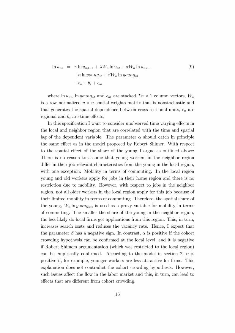
lnunt = lnun;t�1 + �Wn lnunt + �Wn lnun;t�1 (9)
+� ln youngnt + �Wn ln youngnt
+cn + �t + �nt
where lnunt, ln youngnt and �nt are stacked Tn � 1 column vectors, Wn
is a row normalized n � n spatial weights matrix that is nonstochastic andthat generates the spatial dependence between cross sectional units, cn are
regional and �t are time e¤ects.
In this speci�cation I want to consider unobserved time varying e¤ects in
the local and neighbor region that are correlated with the time and spatial
lag of the dependent variable. The parameter � should catch in principle
the same e¤ect as in the model proposed by Robert Shimer. With respect
to the spatial e¤ect of the share of the young I argue as outlined above:
There is no reason to assume that young workers in the neighbor region
di¤er in their job relevant characteristics from the young in the local region,
with one exception: Mobility in terms of commuting. In the local region
young and old workers apply for jobs in their home region and there is no
restriction due to mobility. However, with respect to jobs in the neighbor
region, not all older workers in the local region apply for this job because of
their limited mobility in terms of commuting. Therefore, the spatial share of
the young, Wn ln youngnt, is used as a proxy variable for mobility in terms
of commuting. The smaller the share of the young in the neighbor region,
the less likely do local �rms get applications from this region. This, in turn,
increases search costs and reduces the vacancy rate. Hence, I expect that
the parameter � has a negative sign. In contrast, � is positive if the cohort
crowding hypothesis can be con�rmed at the local level, and it is negative
if Robert Shimers argumentation (which was restricted to the local region)
can be empirically con�rmed. According to the model in section 2, � is
positive if, for example, younger workers are less attractive for �rms. This
explanation does not contradict the cohort crowding hypothesis. However,
such issues a¤ect the �ow in the labor market and this, in turn, can lead to
e¤ects that are di¤erent from cohort crowding.
16

If the spatial e¤ect of the age structure of the working age population is
of importance, we have to consider the bias on � if we neglect �. Let ! be
the parameter for the local e¤ect, when the spatial e¤ect is neglected. The
standard result is then ! = � + ��, where � is a measure for the covariance
of the local and the spatial age structure. I expect the latter to be positive
and � to be negative, which yields a negative bias on !. This might be
an explanation, why Robert Shimer has estimated a negative relationship
between the unemployment rate and the share of the young.
In the analysis I will not discuss the e¤ects of the lagged dependent vari-
able, because these parameters are not important here. These lags serve as
proxies for unobserved e¤ects only.
3.1 Data
I use three di¤erent data sets. First, the original data used in Robert Shimers
(2001) article. He uses the unemployment rate and the share of the working-
age population (ages 16-64) who are aged 16-24 at the US state level. Unem-
ployment rate is taken from the CPS and shares are taken from Census. He
uses annual data for 51 US states and the period 1973 - 1996. The second
data set is taken from the paper by Chris Foote (2007), who extends the data
of Robert Shimer to 2005 and uses the same sources.
The third data set is new. I use the unemployment rate and share of
the young at the US county level. The latter group is considered in three
di¤erent de�nitions: share of the working-age population (ages 15-64) who
are aged 16-24, share of the working-age population who are aged 16-39,
and share of the working-age population who are aged 16-49. With respect
to the �rst share I follow the de�nition of Shimer and Foote and for the
second share I consider the criticism of Carsten Ochsen and Pascal Hetze
(2006). I use this broader de�nition of young and old workers than most
other studies because I believe that many of the individual characteristics
that are relevant to job creation and job destruction, such as quit rates and
productivity changes, alter when workers reach middle age.10 The last share
10For example, Börsch-Supan (2003) showed that the typical age-productivity pro�leusually peaks when workers are in their 40s. The Federal Institute for Employment Re-search in Germany came to the same conclusion.
17

serves as a control group to test if the results are plausible if I use such a
de�nition. The unemployment rate is taken from the BLS and shares are
taken from Census. The analysis considers annual data for 3074 counties
and the period 1998 to 2007.
With respect to the percentages of younger and older people used, there
are considerable di¤erences between regions at the state level and, in partic-
ular, at the county level. The state level data for the period 1973 - 1996 have
an average unemployment rate of 6.3 percentage points (standard deviation
of 2.04) and ranges from 1.9 to 17.4 percentage points. The data extended
to 2005 do not di¤er much: the average unemployment rate is about 5.9
percentage points (standard deviation 1.98) and the range is not di¤erent
from for former. The share of the young (aged 16-24) in the period 1973 -
1996 is on average equal to 0.24 (standard deviation is 0.03) and ranges from
0.16 to 0.33. For the extended period we have an average of 0.23 (standard
deviation of 0.04) and minimum/maximum values as before.
At the county level we have an average unemployment rate of 5.8 (stan-
dard error of 2.69) with a range between 0.7 and 30.6. With respect to the
share of the age cohort 16-24 we get an average of 0.40 (standard error is
0.04) and minimum and maximum values of 0.23 and 0.71. Hence, at the
county level we have much more variation in a shorter time period.
3.2 Econometric Model
Age e¤ects on the unemployment rate are analyzed using mostly macroeco-
nomic data. In this section I provide alternative estimates that allow spatial
e¤ects to be considered using regional data. In order to draw conclusions on
the basis of di¤erent approaches, which should serve as a kind of robustness
check, I estimate the model in three di¤erent ways. First, I apply the usual
within panel estimator with �xed and time e¤ects and robust standard errors.
Second, I use the same estimator and calculate standard errors according the
method provided by John Driscoll and Aart Kraay (1998).11 In addition
11When the assumption of cross-sectional independence is violated, estimates of stan-dard errors are inconsistent, so they are not useful for inference. Driscoll and Kraay (1998)argued that spatial correlations among cross-sections may arise for a number of reasons,ranging from observed common shocks, such as terms of trade or oil shocks, to unobserved
18

to heteroskedasticity this procedure also controls for (serial) autocorrelation
and spatial correlation. In the latter case, however, they use annual averages
over all regions. This does not consider adequate regional correlation, e.g.,
of neighbor regions.
Third, I use an estimator provided by Lung-fei Lee and Jihai Yu (2010).
In this case, the parameters for the time lagged, spatial lagged, and space-
time lagged values of the dependent variables are estimated using a quasi-
maximum likelihood estimator that is extended by a bias correction. To avoid
biased estimates for the lagged e¤ects of the dependent variables, the authors
developed a data transformation approach that has the same asymptotic
e¢ ciency as the quasi-maximum likelihood estimator when n is not relatively
smaller than T . The reason why I use three di¤erent approaches is that
no one of them is free of criticism. In the �rst and second case I have
better standard errors but biased coe¢ cients with respect to the time and
spatial lagged e¤ects of the dependent.12 In the third case the coe¢ cients
are unbiased but the standard errors are probably nor correct.
What about IV estimation? With respect to the causal relationship of
aging and unemployment, both directions are possible. In the supply side�s
"migration e¤ect," young people move into regions with comparatively low
unemployment rates, and this movement results in an increased percentage
of older workers in regions with high unemployment rates. In the demand
side e¤ect, �rms could prefer younger workers, and in regions with a larger
percentage of older workers, the unemployment rate is higher. With respect
to migration, one could argue that there are two opposing e¤ects that bal-
ance regional unemployment rates to a certain extent. First, young people
choose regions with comparatively low unemployment rates, which decrease
the market tightness in the chosen region. Second, given that uy > uo, emi-
gration should decrease the overall unemployment rate. For Robert Shimers
and Chris Footes data I also estimate the model with an IV estimator using
contagion or neighborhood e¤ects. Building on the non-parametric heteroskedasticity andautocorrelation consistent covariance matrix estimation technique, they showed how thisapproach can be extended to a panel setting with cross-sectional dependence.
12See, for example, Nickell (1981) with respect to the asymptotic bias of OLS estimationusing the time lagged e¤ect and Kelejian and Prucha (1998) for information on biased OLSestimates when spatial lagged e¤ects are considered.
19

the same instrument as they do; the local lagged birth rates. For the county
data, however, I do not estimate the model with an IV estimator because
appropriate instruments are not available at the county level. In addition,
birth rates are probably not a suitable instrument at the county level because
family movements can a¤ect this variable much more than at the state level.
Without additional IV estimates at the county level, however, we have to be
careful when interpreting the results.
3.3 Results
Table 2 provides the results of the three preferred estimators� robust, D&K,
and L&Y� using the original data from Robert Shimers article. With re-
spect to the speci�cation without the spatial e¤ect of the young, I �nd that
the local younger labor force is negatively related to the local unemployment
rate, when the speci�cation "robust" is considered. Hence, using this estima-
tor I get results that are comparable to those of Robert Shimer. However, the
e¤ect is not statistical signi�cant for the second and third estimator. When
I consider the spatial share of the young, the e¤ects for the local share of
the young are insigni�cant in all cases. I �nd a similar e¤ect for the per-
centage of younger workers in the surrounding labor market. Given that
younger workers are more mobile than older workers, aging reduces the share
of regional mobile workers, and this reduction, in turn, increases the local
unemployment rate. However, this e¤ect is not signi�cant.
Table 2 about here
The original data used in the paper by Chris Foote are used in the es-
timates provided in table 3. In contrast to the results in table 2 no e¤ect
is signi�cant. This is surprising to some extend, since the only di¤erence is
the extension of the considered period. However, the results are in line with
Chris Footes conclusion whereby overall there is no signi�cant relationship
between the local unemployment rate and the local share of the young. That
this applies to the spatial share of the young as well.
Table 3 about here
20
The results in the tables 2 and 3 can be interpreted in di¤erent ways. Of
course, it is possible that the di¤erence between younger and older workers is
too small to be signi�cant. However, it is also possible that opposing e¤ects
cancel out each other. For example, if younger workers undertake job search
more intensively but older workers are more productive, the overall e¤ect
can be small and insigni�cant. A third explanation is related to the size of
the regions. Within a state are also a lot of spatial mobile workers that are
measured as local workers. As mentioned above, neglecting the share of the
young in the neighbor region yield a negative bias on the share of the young
in the local region. At the state level, however, I cannot distinguish these two
groups within a state. Hence, the true local e¤ect can also be positive. In
addition, the share of the young in a neighbor state might be less related to a
local state than, for example, the share of the young in a neighbor and local
county. If the explanation related to the wrong regional size is relevant, the
results are expected to be di¤erent when county level data are considered.
In the next step I therefore focus on counties as regions and use in the �rst
case the same de�nition of the young as Robert Shimer and Chris Foote.
The results in table 4 are related US county level data. Now, the �rst
and third speci�cation yield signi�cant positive e¤ects. The second e¤ect is
signi�cant only at the 10 percent level, but with only ten years the correction
for spatial correlation in the variance covariance matrix could be misleading.
When I now consider the spatial share of the young as additional variable,
the e¤ects of the local share remain practically unchanged. In contrast, the
spatial e¤ect is not signi�cant. The results in table 4 are now compatible
with the cohort crowding hypothesis. However, is it also possible, that the
results re�ect di¤erences in characteristics of younger and older workers. As
discussed above, young workers are more mobile, have higher turnover rates,
and could be less productive.
Table 4 about here
I now want to consider another de�nition of younger workers. As argued
above, many talented young people do not have �nished their education
when 24 years old and do not have some basic job experiences. Hence, I
de�ne the young as those between 16 and 39 years old. Table 5 provides
21
the results for the US county data. The results for the local share of the
young are similar to those provided in table 4. However, in this case all
estimated e¤ects are signi�cant at the 1 percent level. The spatial e¤ect
of the young is now signi�cant negative. The �rst result is an indication
of higher productivity among older workers and the second an indication
that, the higher the number of younger job seekers in the neighbor district,
the more jobs will be created in the local labor market.13 With respect
to the latter e¤ect I conclude that spatial mobility in terms of commuting
is of importance for the local unemployment rate. The larger the share of
young workers in the neighbor regions, the lower the local unemployment
rate. One reason why I yield this signi�cant e¤ect here but not in the former
speci�cation is that the match quality with experienced younger workers is
higher than with unexperienced ones. This makes the spatial e¤ect stronger.
Table 5 about here
As discussed above, this second spatial age e¤ect does not mean that the
productivity di¤erential between younger and older workers is reversed since
it is not possible that a worker from the spatial region will always have higher
productivity because every region is both a neighbor and a local district in
the estimates; instead, it appears that the estimated e¤ect re�ects the spatial
mobility of workers in the surrounding area. The outcome of this e¤ect is
comparable to the standard e¤ect of on-the-job searches on job creation; that
is, the more people demanding new jobs, the lower the search costs for �rms
and this lower cost increases job creation.
However, if this is the case, why does the local labor supply yield to
an opposing e¤ect? One explanation is that both younger and older job
seekers in the local labor market apply for vacant jobs in the region, as the
theoretical model assumed. Hence, if aging is restricted to the local area,
regional mobility no longer in�uences job creation and, if aging occurs in
the local and neighbor regions in a similar way, the overall number of job
13These �ndings may improve our understanding of the di¤erences between regional andnational level �ndings. As Robert Shimer (2001) emphasized in his study of the impact ofyoung workers on the aggregate labor market, the relative importance of competing e¤ectsat di¤erent levels of aggregation is puzzling. Our results may provide a key to the puzzle.
22
seekers is reduced; thus, search costs increase and job creation declines in
both regions because of their spatial interaction.
As a robustness check I now consider a cut o¤ for younger and older
people that is at an even higher age than before. Here, the young are de�ned
as those between 16 and 49 years old. I expect that both the local and the
spatial e¤ect will be less strong and less or not signi�cant. Table 6 provides
the results. Only the local e¤ect when using the estimator suggested by
Lee and Yu is signi�cant. However, as discussed earlier, the corresponding
standard errors are misleading if the residuals exhibit a speci�c pattern.14
That is, we should be careful when interpreting the results when no other
estimator yields signi�cant results. To sum up, the results provided in table
6 indicate that both the local and the spatial e¤ect diminish when I increase
the cut o¤ between young and old.
Table 6 about here
3.4 Further Estimates
This section provides some IV results that are comparable to tables 2 and 3.
Since it is plausible that the parameters that correspond to aging su¤er from
a simultaneous equation bias, I ran additional regressions and instrument
the percentage of young people in the local and surrounding region by (time)
lagged birth rates and by the spatial lag of (time) lagged birth rates. I esti-
mate the equations with a �xed e¤ects instrumental variable (IV) estimator.
Table 7 provides the estimates. According to the estimates, the simultaneous
equation bias seems to have a negligible e¤ect on the size of the parameters.
With respect to the shorter period, I derive the same result for the speci�ca-
tion without a spatial age e¤ect, and the e¤ect is still signi�cant at the 5%
level. All other e¤ects are not signi�cant. Overall, my IV estimates for the
US at the state level, using Robert Shimers and Chris Footes data, lead not
to conclusions that do deviate from the �ndings above. This is in accordance
with Robert Shimers �ndings.
Table 7 about here14The variance covariance matrix is estimated under the null of white noise in the
residuals.
23

According to the results at the state level, I conclude that IV estimates are
not necessary to improve the estimates. Unfortunately, I cannot do the same
regression exercise with the county level data. If this conclusion holds for this
level of aggregation as well, the results presented in this paper are robust.
However, this is speculative and we have to be carefully when interpreting
the results at the county level.
4 Conclusions
In this paper, I examined the relationship between the change in the (spa-
tial) age structure of the working age population and unemployment at the
regional level using both a theoretical and an empirical model. In the em-
pirical part I consider di¤erent data for the US at the regional level. Based
on my proxy for aging� the percentage of younger people in the working
age population� ongoing aging will cause two opposing e¤ects when I use
US county level data and a broader de�nition of the young. First, aging
in the local labor market decreases unemployment, while aging in the sur-
rounding areas has a positive e¤ect on the unemployment rate in the local
district. My interpretation is that an aging labor force decreases the match-
ing e¢ ciency but local �rms respond positively to the local percentage of
older workers because of productivity di¤erences between older and younger
workers. However, the results are also compatible with the cohort crowding
hypothesis, which I do not call into question. The e¤ect of aging in the sur-
rounding area di¤ers from the local e¤ect because younger workers are more
mobile (in terms of commuting) than older workers are.
My results also suggest that regions with a larger percentage of older
workers have to attract younger ones, and this can have two e¤ects� the
matching e¢ ciency increases and �rms become more willing to create jobs�
both of which decrease the regional unemployment rate. In addition, it ap-
pears to be necessary for the regional mobility of older people in the labor
market to increase in order to mitigate the estimated e¤ects of aging on
unemployment.
Using state level data like Robert Shimer and Chris Foote yield no sup-
port for an e¤ect of aging on unemployment. My interpretation is that this
24
level of disaggregation is too high to di¤erentiate the two opposing e¤ects of
productivity and mobility. In addition, the results at the county level under-
line that commuting is important to reduce local unemployment. However,
the results (may) depend on the de�nition of the young.
Appendix
E¤ects of Aging on the Beveridge Curve (BC): The e¤ects on the localBC of eq. (2) arises through a change in the age composition of job seekers.
The �rst e¤ect comes from a change in the local age composition of the job
seekers available to local �rms:
@ul
@pl
����@�l=0
=�uly � ulo
�(10)
+pl
�l @q
l(�l;�pl)@�pl
�ly�l+~�n
+�n @qn(�n;�pn)@�pn
�ly�n+~�l
!0@ �ulysl+� ly+�
lql(�l;�pl)+�nqn(�n;�pn)
� �ulosl+� lo+�
lql(�l;�pl)+�nqn(�n;�pn)
1A+
�l @q
l(�l;�pl)@�pl
�ly�l+~�n
+�n @qn(�n;�pn)@�pn
�ly�n+~�l
!�ulo
sl + � lo + �lql(�l; �pl) + �nqn(�n; �pn)
:
The �rst term is positive if � y > � o. A higher percentage of older workers
reduces the labor turnover such that fewer job-worker pairs must be matched:
the BC shifts inwards. The second and third terms represent the (spatial)
e¤ect of the change in matching e¢ ciency; this e¤ect is negative because
a decline in pl increases the average duration of the search on either side;
hence, the aging e¤ect shifts the local BC outwards. With respect to a new
equilibrium in the local BC, it follows that aging has ambiguous e¤ects. The
�rst and second term would be zero if � y = � o, however, even in this case,
aging increases unemployment because the third term still shifts the BC
outwards.
With respect to the spatial age e¤ect, the local unemployment rate re-
sponds to a change in pn according to:
25

@ul
@pn
����@�l=0
= pn
�l @q
l(�l;�pl)@�pl
�ny�l+~�n
+�n @qn(�n;�pn)@�pn
�ny�n+~�l
!0@ �ulysl+� ly+�
lql(�l;�pl)+�nqn(�n;�pn)
� �ulosl+� lo+�
lql(�l;�pl)+�nqn(�n;�pn)
1A(11)+
�l @q
l(�l;�pl)@�pl
�ny�l+~�n
+�n @qn(�n;�pn)@�pn
�ny�n+~�l
!�ulo
sl + � lo + �lql(�l; �pl) + �nqn(�n; �pn)
.
Both terms on the right-hand side are similar to the second and third
term in eq. (10), and the interpretation is the same.
E¤ects of Aging on job creation (JC):To analyze the e¤ects of agingon the local job creation condition (7), we reorganize (7) and make use of
an implicit di¤erentiation. The two arguments in ql are �l and �pl. For
F��l; �pl
�= 0, we di¤erentiate �l with respect to �pl and make use of �@F=@�pl
@F=@�l:
@�l
@�pl= �
ql(�l; �pl)�J ly � J lo
�+@ql(�l;�pl)
@pl
24 �plJ ly
�1� @J ly
@ql(�l;�pl)
ql(�l;�pl)J ly
�+�1� �pl
�J lo
�1� @J lo
@ql(�l;�pl)
ql(�l;�pl)J lo
� 35�pl�J ly
@ql(�l;�pl)
@�l+ ql(�l; �pl)
@J ly@�l
�+�1� �pl
� �J lo
@ql(�l;�pl)
@�l+ ql(�l; �pl)@J
lo
@�l
� . (12)
The denominator of (12) is negative because J li@ql(�l;�pl)
@�l+ ql(�l; �pl)
@J li@�l
is
negative if elasticity @J li@ql(�l;�pl)
ql(�l;�pl)
J liis smaller than unity, with i 2 fl; og.
Because @J li@ql(�l;�pl)
< 0, we have a strict negative denominator; hence, the sign
of (12) depends on the numerator. We have @�l
@�pl> 0 if the numerator is
positive or the other way around. With @J li@ql(�l;�pl)
< 0, it is clear that the
second term in the numerator becomes positive. Hence, (12) is positive if the
�rst term is positive as well, that is, if J ly > Jlo; if not, the sign of
@�l
@�pldepends
on whether the �rst or the second term in (12) dominates the total e¤ect.
26

5 References
Autor, D.H.; Levy, F.; Murnane, J.R., 2003, The Skill Content of Recent
Technological Change: An Empirical Exploration, Quarterly Journal
of Economics 118(4), 1279-1334.
Bartel, A.P., Sicherman, N., 1993, Technological Change and Retirement
Decisions of Older Workers, Journal of Labor Economics 11, 162-193.
Blanchard, O., Diamond, P., 1989, The Beveridge Curve, Brookings Papers
on Economic Activity 1, 1-60.
Bloom, D.E.; Freeman, R.B.; Korenman, S., 1987, The Labour Market Con-
sequences of Generational Crowding, European Journal of Population
3, 131-176.
Börsch-Supan, A., 2003, Labor Market E¤ects of Population Aging, Labour
17, 5-44.
Brücker, H., Trübswetter, P., 2007, Do the Best goWest? An Analysis of the
Self-Selection of Employed East-West Migrants in Germany, Empirica
34, 371-395.
Burda, M.C., Pro�t, S., 1996, Matching across Space: Evidence on Mobility
in the Czech Republic, Labour Economics 3(3), 255-278.
Burgess, S.M. 1993, A Model of Competition between Unemployed and
Employed Searchers: An Application to the Unemployment Out�ows
in Britain, Economic Journal 103, 1190-1204.
Burgess, S.M., Pro�t, S., 2001, Externalities in the Matching of Workers
and Firms in Britain, Labour Economics 8(3), 313-333.
Coles, M., Smith, E., 1996, Cross-Section Estimation on the Matching Func-
tion: Evidence from England and Wales, Economica 63, 589-597.
Daniel, K., Heywood, J.S., 2007, The Determinants of Hiring Older Work-
ers: UK Evidence, Labour Economics 14, 35-51.
27

Davis, S.J.; Haltiwanger, J.C.; Schuh, S., 1996, Job Creation and Job De-
struction, MIT Press, Cambridge, Massachusetts.
Driscoll, J.C., Kraay, A.C., 1998, Consistent Covariance Matrix Estima-
tion with Spatially Dependent Panel Data, Review of Economics and
Statistics 80, 549-560.
Fahr, R., Sunde, U., 2005, Regional Dependencies in Job Creation: An
E¢ ciency Analysis for West Germany, IZA, Discussion Paper No. 1660.
Fallick, B., Fleischman, C., 2004, Employer-to-Employmer Flows in the U.S.
Labor Market: The Complete Picture of Gross Worker Flows, Federal
Reserve Board, Finance and Economics Working Paper Series 2004-34.
Flaim, P., 1979, The E¤ect of Demographic Change on the Nation�s Unem-
ployment Rate, Monthly Labor Review CII, 13-23.
Flaim, P., 1990, Population Changes, the Baby Boom and the Unemploy-
ment Rate, Monthly Labor Review CXIII, 3-10.
Foote, C.L., 2007, Space and Time in Macroeconomic Panel Data: Young
Workers and State-Level Unemployment Revisited, Federal Reserve
Bank of Boston, Working Paper No. 07-10.
Gordon, R., 1982, In�ation, Flexible Exchange Rates, and the Natural Rate
of Unemployment, in M. Baily ed, Workers, Jobs and In�ation, Wash-
ington, DC, Brookings Institution, 89-152.
Gracia-Diez, M., 1989, Compositional Changes of the Labor Force and
the Increase of the Unemployment Rate: An Estimate for the United
States, Journal of Business & Economic Statistics 7(2), 237-243.
Haltiwanger, J.C.; Lane, J.I.; Spletzer, J.R., 1999, Productivity Di¤erences
Across Employers: The Roles of Employer Size, Age, and Human Cap-
ital, American Economic Review 89(2), 94-98.
Hellerstein, J.K.; David, N.; Troske, K.R., 1999, Wages, Productivity and
Workers Characteristics: Evidence From Plant Level Production Func-
tion and Wage Equations, Journal of Labor Economics 17, 409-446.
28

Ochsen, C., Hetze, P., 2006, Age E¤ects on Equilibrium Unemployment,
Rostock Center for the Study of Demographic Change, Discussion Pa-
per No 1.
Hujer, R.; Rodrigues, P.J.M.; Wolf, K., 2009, Estimating the Macroeco-
nomic E¤ects of Active Labour Market Policies using Spatial Econo-
metric Methods, International Journal of Manpower, forthcoming.
Hunt, J., 2000, Why do People Still Live in East Germany, NBER Working
Paper Series 7564.
Hutchens, R.M., 2001, Employer Surveys, Employer Policies, and Future
Demand for Older Workers, Paper prepared for the Roundtable on the
Demand for Older Workers, The Brookings Institute.
Kelejian, H.H., Prucha, I.R., 1998, Estimation of Spatial Regression Models
with Autoregressive Errors by Two-Stage Least Squares Procedures: A
Serious Problem, International Regional Science Review 20, 103-111.
Korenman, S.; Neumark, D., 2000, Cohort Crowding and Youth Labor
Markets: A Cross-National Analysis, in D. Blanch�ower and R.B. Free-
man eds, Youth Unemployment and Joblessness in Advanced Countries,
Chicago, University of Chicago Press, 57-105.
Lee, L.-F., Yu, J., 2010, A Spatial Dynamic Panel Data Model with Both
Time and Individual Fixed E¤ects, Econometric Theory 26(2), 564-597.
Lindley, J.; Upward, R.; Wright, P., 2002, Regional Mobility and Unemploy-
ment Transitions in the UK and Spain, Leverhulme Centre for Research
on Globalisation and Economic Policy, University of Nottingham.
Nickell, S.J., 1981, Biases in Dynamic Models with Fixed E¤ects, Econo-
metrica 59, 1417-1426.
Patacchini, E.; Zenou, Y., 2007, Spatial Dependence in Local Unemploy-
ment Rates, Journal of Economic Geography 7, 169-191.
29

Petrongolo, B., Pissarides, C.A., 2001, Looking into the Black Box: A Sur-
vey of the Matching Function, Journal of Economic Literature 39 (2),
390-431.
Petrongolo, B., Wasmer, É., 1999, Job Matching and Regional Spillovers
in Britain and France, in Developments Récents et Économie Spatiale:
Employ, Concurrence Spatiale et Dynamiques Régionales, M.Catain,
J.-Y Lesieur, Y. Zenou eds., Paris, Economica, 39-54.
Pissarides, C.A., 1994, Search Unemployment with On-The-Job Search, Re-
view of Economic Studies 61(3), 457-475.
Perry, G., 1970, Changing Labor Markets and In�ation, Brookings Papers
on Economic Activity, 411-441.
Pissarides, C.A., 2000, Equilibrium Unemployment Theory, MIT Press,
Cambridge MA.
Pissarides, C.A., Wadsworth, J., 1994, On-the-Job Search: Some Empirical
Evidence from Britain, European Economic Review 38, 385-401.
Shimer, R., 2001, The Impact of Young Workers on the Aggregate Labor
market, Quarterly Journal of Economics 116(3), 969-1007.
Yu, J.; de Jong, R.; Lee, L.-F., 2008, Quasi-Maximum Likelihood Estima-
tors for Spatial Dynamic Panel Data with Fixed e¤ects when Both n
and T are Large, Journal of Econometrics 146, 118-134.
6 Figure and Tables
Table 1: Main Results in the Two StudiesRob Shimer Chris Foote
share of the young -1.246z -0.420
Note:z=1% level of signi�cance
30

Figure 1: E¤ects of Aging on the Search Equilibrium
Figure 2: Share of the 15-24 Years Old and Smoothed Unemployment Rate,USA, 1960-2010
31

Figure 3: Share of the 15-39 Years Old and Smoothed Unemployment Rate,USA, 1960-2010
Table 2: Results for Robert Shimers US State Level Data(1) (2) (3) (4) (5) (6)
Variables robust D & K L & Y robust D & K L & Y
share of the young -0.217y -0.217 -0.123 -0.201] -0.201 -0.122
spatial share of the young -0.140 -0.140 -0.035
Notes: Dependent variable: log of unemployment rate; regression include: timelagged e¤ect of the dependent, spatial lagged e¤ect of the dependent, spatial and time
lagged e¤ect of the dependent and (regional) �xed and time e¤ects; methods: robust
= within �xed e¤ects estimator with robust standard errors, D&K = within �xed
e¤ects estimator with Driscoll and Kraay standard errors, L&Y = quasi maximum
likelihood estimator with bias correction according to Lee and Yu; observations: 1,290;
signi�cance: z=1%, y=5%, ]=10%.
32
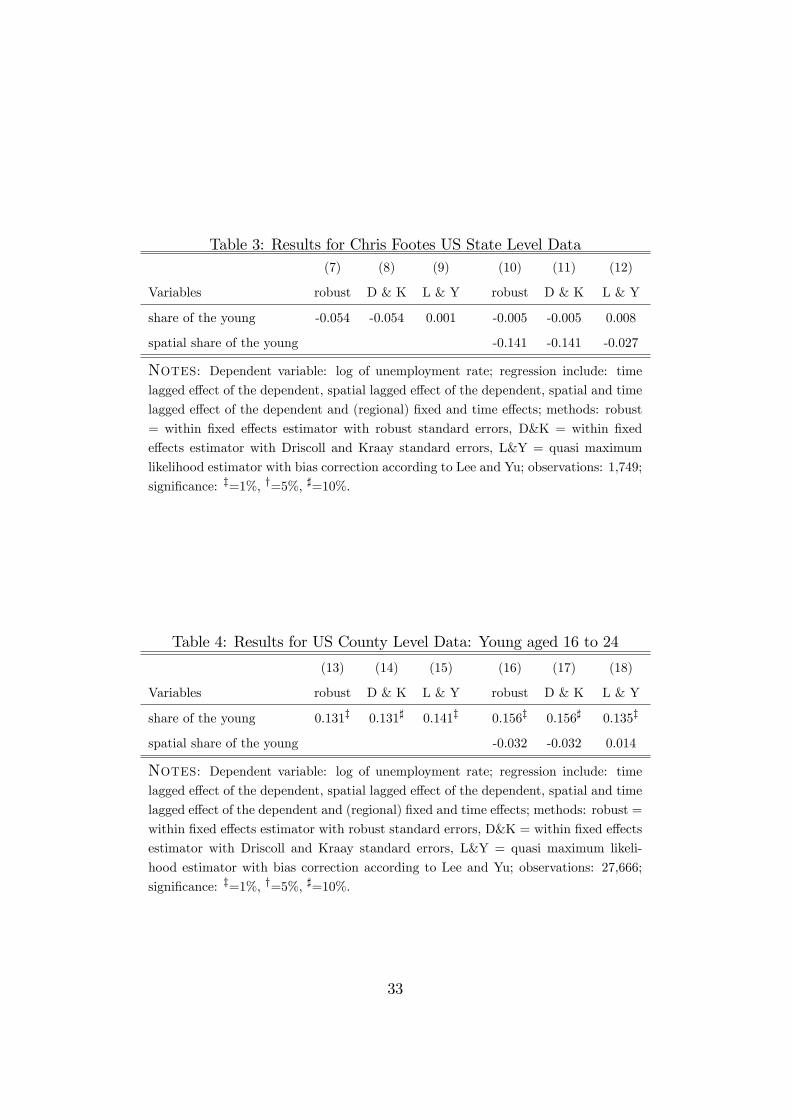
Table 3: Results for Chris Footes US State Level Data(7) (8) (9) (10) (11) (12)
Variables robust D & K L & Y robust D & K L & Y
share of the young -0.054 -0.054 0.001 -0.005 -0.005 0.008
spatial share of the young -0.141 -0.141 -0.027
Notes: Dependent variable: log of unemployment rate; regression include: timelagged e¤ect of the dependent, spatial lagged e¤ect of the dependent, spatial and time
lagged e¤ect of the dependent and (regional) �xed and time e¤ects; methods: robust
= within �xed e¤ects estimator with robust standard errors, D&K = within �xed
e¤ects estimator with Driscoll and Kraay standard errors, L&Y = quasi maximum
likelihood estimator with bias correction according to Lee and Yu; observations: 1,749;
signi�cance: z=1%, y=5%, ]=10%.
Table 4: Results for US County Level Data: Young aged 16 to 24
(13) (14) (15) (16) (17) (18)
Variables robust D & K L & Y robust D & K L & Y
share of the young 0.131z 0.131] 0.141z 0.156z 0.156] 0.135z
spatial share of the young -0.032 -0.032 0.014
Notes: Dependent variable: log of unemployment rate; regression include: timelagged e¤ect of the dependent, spatial lagged e¤ect of the dependent, spatial and time
lagged e¤ect of the dependent and (regional) �xed and time e¤ects; methods: robust =
within �xed e¤ects estimator with robust standard errors, D&K = within �xed e¤ects
estimator with Driscoll and Kraay standard errors, L&Y = quasi maximum likeli-
hood estimator with bias correction according to Lee and Yu; observations: 27,666;
signi�cance: z=1%, y=5%, ]=10%.
33
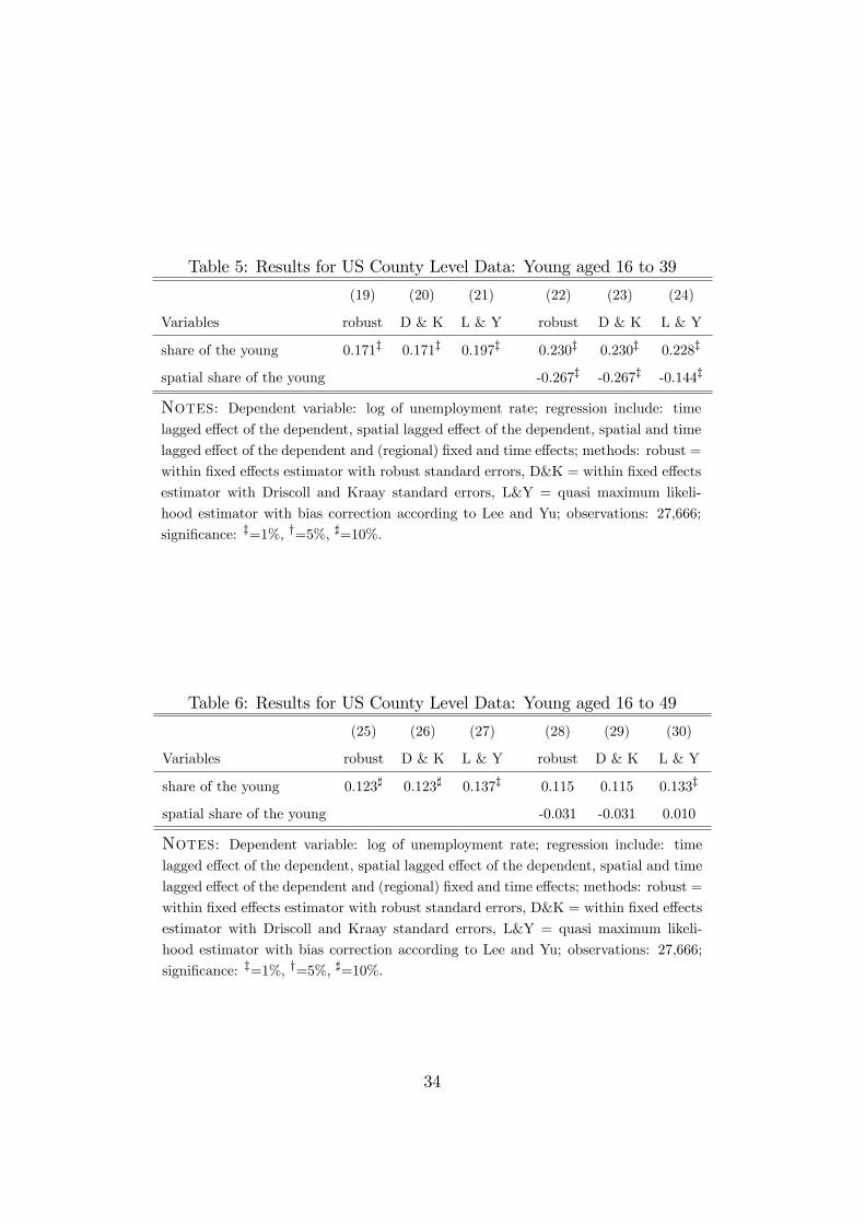
Table 5: Results for US County Level Data: Young aged 16 to 39
(19) (20) (21) (22) (23) (24)
Variables robust D & K L & Y robust D & K L & Y
share of the young 0.171z 0.171z 0.197z 0.230z 0.230z 0.228z
spatial share of the young -0.267z -0.267z -0.144z
Notes: Dependent variable: log of unemployment rate; regression include: timelagged e¤ect of the dependent, spatial lagged e¤ect of the dependent, spatial and time
lagged e¤ect of the dependent and (regional) �xed and time e¤ects; methods: robust =
within �xed e¤ects estimator with robust standard errors, D&K = within �xed e¤ects
estimator with Driscoll and Kraay standard errors, L&Y = quasi maximum likeli-
hood estimator with bias correction according to Lee and Yu; observations: 27,666;
signi�cance: z=1%, y=5%, ]=10%.
Table 6: Results for US County Level Data: Young aged 16 to 49
(25) (26) (27) (28) (29) (30)
Variables robust D & K L & Y robust D & K L & Y
share of the young 0.123] 0.123] 0.137z 0.115 0.115 0.133z
spatial share of the young -0.031 -0.031 0.010
Notes: Dependent variable: log of unemployment rate; regression include: timelagged e¤ect of the dependent, spatial lagged e¤ect of the dependent, spatial and time
lagged e¤ect of the dependent and (regional) �xed and time e¤ects; methods: robust =
within �xed e¤ects estimator with robust standard errors, D&K = within �xed e¤ects
estimator with Driscoll and Kraay standard errors, L&Y = quasi maximum likeli-
hood estimator with bias correction according to Lee and Yu; observations: 27,666;
signi�cance: z=1%, y=5%, ]=10%.
34
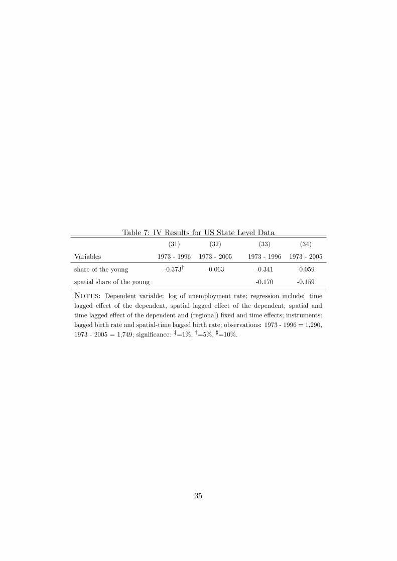
Table 7: IV Results for US State Level Data(31) (32) (33) (34)
Variables 1973 - 1996 1973 - 2005 1973 - 1996 1973 - 2005
share of the young -0.373y -0.063 -0.341 -0.059
spatial share of the young -0.170 -0.159
Notes: Dependent variable: log of unemployment rate; regression include: timelagged e¤ect of the dependent, spatial lagged e¤ect of the dependent, spatial and
time lagged e¤ect of the dependent and (regional) �xed and time e¤ects; instruments:
lagged birth rate and spatial-time lagged birth rate; observations: 1973 - 1996 = 1,290,
1973 - 2005 = 1,749; signi�cance: z=1%, y=5%, ]=10%.
35