RELATIONAL ALGEBRA and Computer Assignment 1

Prof. Sin-Min LEE

Department of Computer Science

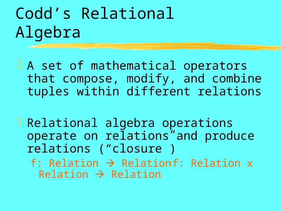
Codd’s Relational Algebra

A set of mathematical operators that compose, modify, and combine tuples within different relations

Relational algebra operations operate on relations and produce relations (“closure”)f: Relation Relation f: Relation x

Relation Relation

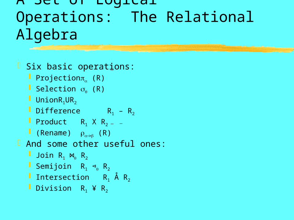
A Set of Logical Operations: The Relational Algebra

Six basic operations: Projection (R) Selection (R) Union R1UR2

Difference R1 – R2

Product R1 X R2

(Rename) (R)And some other useful ones:

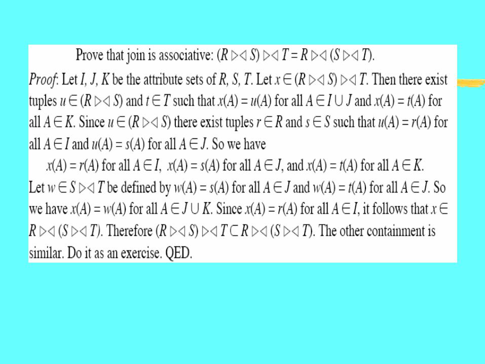
Join R1 ⋈ R2

Semijoin R1 ⊲ R2

IntersectionR1 Å R2 Division R1 ¥ R2

Data Instance for Operator Examples

sid name

1 Jill

2 Qun

3 Nitin

fid name

1 Ives

2 Saul

8 Roth

sid exp-grade

cid

1 A 550-0105

1 A 700-1005

3 C 501-0105

cid subj sem

550-0105

DB F05

700-1005

AI S05

501-0105

Arch F05fid

cid

1 550-0105

2 700-1005

8 501-0105

STUDENT Takes COURSE

PROFESSOR Teaches

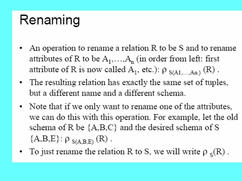
Rename,

The rename operator can be expressed several ways: The book has a very odd definition that’s not

algebraic An alternate definition:

(x) Takes the relation with schema Returns a relation with the attribute

list

Rename isn’t all that useful, except if you join a relation with itself

Why would it be useful here?

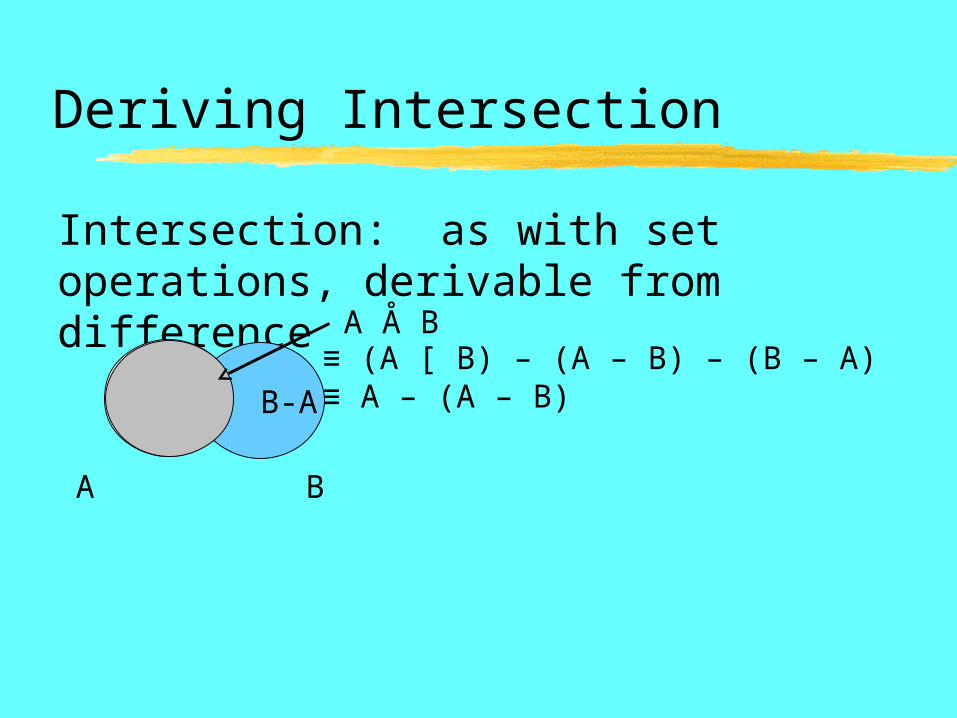
Deriving Intersection

Intersection: as with set operations, derivable from difference

A-B B-A

A B

A Å B≡ (A [ B) – (A – B) – (B – A)≡ A – (A – B)

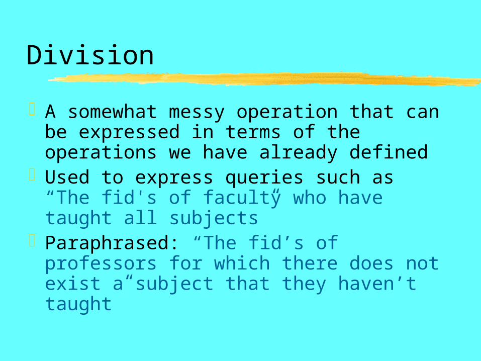
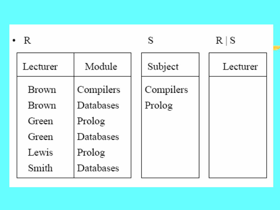
Division

A somewhat messy operation that can be expressed in terms of the operations we have already defined

Used to express queries such as “The fid's of faculty who have taught all subjects”

Paraphrased: “The fid’s of professors for which there does not exist a subject that they haven’t taught”

Division Using Our Existing OperatorsAll possible teaching assignments:

Allpairs:

NotTaught, all (fid,subj) pairs for which professor fid has not taught subj:

Answer is all faculty not in NotTaught:

fid,subj (PROFESSOR x subj(COURSE))

Allpairs - fid,subj(Teaches COURSE)⋈fid(PROFESSOR) - fid(NotTaught)

´ fid(PROFESSOR) - fid(fid,subj (PROFESSOR x subj(COURSE)) -

fid,subj(Teaches COURSE))⋈

Division: R1 R2

Requirement: schema(R1) ÷schema(R2)Result schema: schema(R1) – schema(R2)“Professors who have taught all courses”:

What about “Courses that have been taught by all faculty”?

fid (fid,subj(Teaches ⋈ COURSE) subj(COURSE))

DIVISION- The division operator is used for queries which involve the

‘all’ qualifier such as “Find the names of sailors who have reserved all boats”.

- The division operator is a bit tricky to explain, and perhaps best approached through examples as will be done here.

Cartesian Product (R1 × R2) combines two relations by concatenating their tuples together, evaluating all possible combinations. If the name of a column is identical for two relations, this ambiguity is resolved by attaching the name of each relation to a column. e.g., Emp × Dept (SS#, name, age, salary, Emp.dno, Dept.dno, dname, floor,

mgrSS#) If t(Emp) and t(Dept) is the cardinality of the Employee and Dept

relations respectively, then the cardinality of Emp × Dept is: t(Emp) × t(Dept)

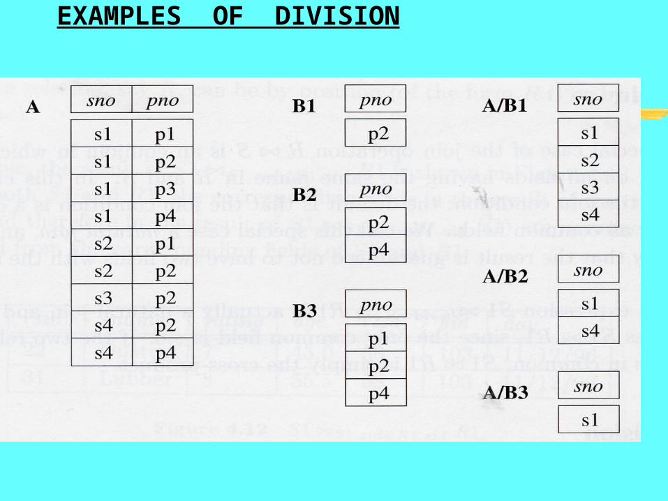
EXAMPLES OF DIVISION

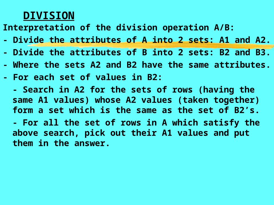
DIVISIONInterpretation of the division operation A/B:- Divide the attributes of A into 2 sets: A1 and A2.- Divide the attributes of B into 2 sets: B2 and B3.- Where the sets A2 and B2 have the same

attributes.- For each set of values in B2:

- Search in A2 for the sets of rows (having the same A1 values) whose A2 values (taken together) form a set which is the same as the set of B2’s.- For all the set of rows in A which satisfy the above search, pick out their A1 values and put them in the answer.

DIVISIONExample: Find the names of sailors who have reserved all

boats:(1) A = sid,bid(Reserves). A1 = sid(Reserves) A2 =

bid(Reserves)

(2) B2 = bid(Boats) B3 is the rest of B.

Thus, B2 ={101, 102, 103, 104}(3) Find the rows of A such that their A.sid is the same

and their combined A.bid is the set B2. Thus we find A1 = {22}

(4) Get the set of A2 corresponding to A1: A2 = {Dustin}

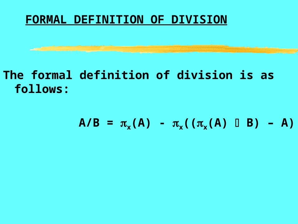
FORMAL DEFINITION OF DIVISION

The formal definition of division is as follows:

A/B = x(A) - x((x(A) B) – A)

CARTESIAN PRODUCT (Cont…)Example:

Emp table:

Dept table:

345 John Doe 23 25,000 1943 Jane Java 25 28,000 2876 Joe SQL 22 32,000 1

SS# Name age salary dno

1 Toy 1 3452 Sho

e2 943

dno dname floor mgrSS#

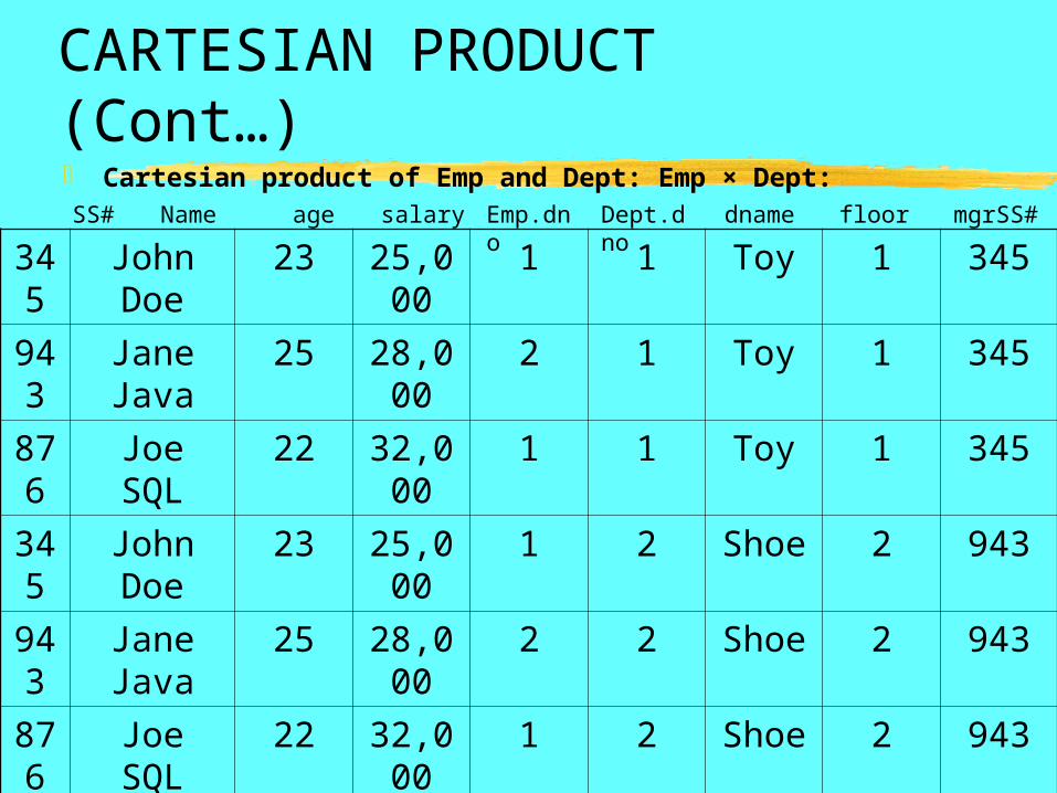
CARTESIAN PRODUCT (Cont…) Cartesian product of Emp and Dept: Emp × Dept:

345

John Doe

23 25,000

1 1 Toy 1 345

943

Jane Java

25 28,000

2 1 Toy 1 345

876

Joe SQL 22 32,000

1 1 Toy 1 345

345

John Doe

23 25,000

1 2 Shoe 2 943

943

Jane Java

25 28,000

2 2 Shoe 2 943

876

Joe SQL 22 32,000

1 2 Shoe 2 943

SS# Name age salary Emp.dno Dept.dno dname floor mgrSS#

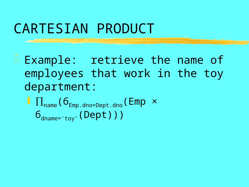
CARTESIAN PRODUCT

Example: retrieve the name of employees that work in the toy department:

CARTESIAN PRODUCT

Example: retrieve the name of employees that work in the toy department: ∏name(бEmp.dno=Dept.dno(Emp ×

бdname=‘toy’(Dept)))

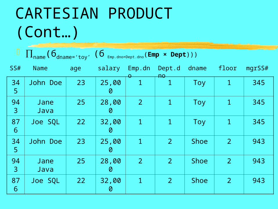
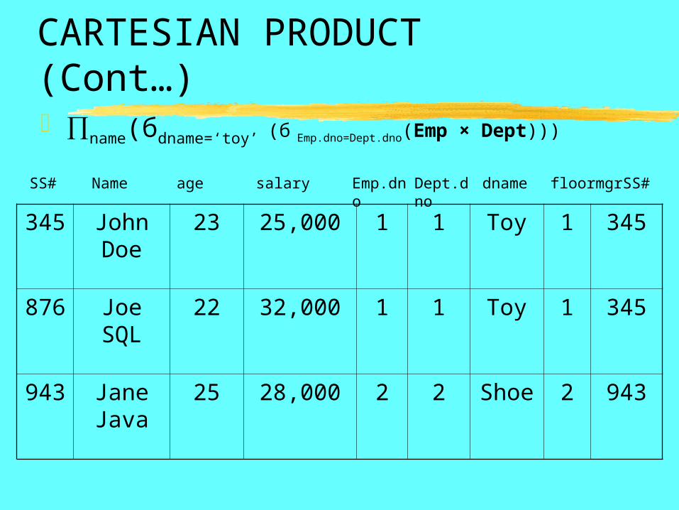
CARTESIAN PRODUCT (Cont…)∏name(бdname=‘toy’ (б Emp.dno=Dept.dno(Emp × Dept)))

345 John Doe 23 25,000 1 1 Toy 1 345

943 Jane Java 25 28,000 2 1 Toy 1 345

876 Joe SQL 22 32,000 1 1 Toy 1 345

345 John Doe 23 25,000 1 2 Shoe 2 943

943 Jane Java 25 28,000 2 2 Shoe 2 943

876 Joe SQL 22 32,000 1 2 Shoe 2 943

SS# Name age salary Emp.dno Dept.dno dname floor mgrSS#

CARTESIAN PRODUCT (Cont…)∏name(бdname=‘toy’ (б Emp.dno=Dept.dno(Emp × Dept)))

345 John Doe

23 25,000 1 1 Toy 1 345

876 Joe SQL

22 32,000 1 1 Toy 1 345

943 Jane Java

25 28,000 2 2 Shoe 2 943

SS# Name age salary Emp.dno Dept.dno dname floor mgrSS#

CARTESIAN PRODUCT (Cont…) ∏name(бdname=‘toy’ (б Emp.dno=Dept.dno(Emp × Dept)))

345 John Doe

23 25,000 1 1 Toy 1 345

876 Joe SQL 22 32,000 1 1 Toy 1 345

SS# Name age salary Emp.dno Dept.dno dname floor mgrSS#

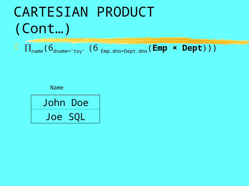
CARTESIAN PRODUCT (Cont…) ∏name(бdname=‘toy’ (б Emp.dno=Dept.dno(Emp × Dept)))

John Doe

Joe SQL

Name

EQUALITY JOIN, NATURAL JOIN, JOIN, SEMI-JOIN

Equality join connects tuples from two relations that match on certain attributes. The specified joining columns are kept in the resulting relation. ∏name(бdname=‘toy’(Emp Dept)))

Natural join connects tuples from two relations that match on the specified common attributes ∏name(бdname=‘toy’(Emp Dept)))

How is an equality join between Emp and Dept using dno different than a natural join between Emp and Dept using dno? Equality join: SS#, name, age, salary, Emp.dno, Dept.dno, … Natural join: SS#, name, age, salary, dno, dname, …

Join is similar to equality join using different comparison operators A S op = {=, ≠, ≤, ≥, <, >} att op att

(dno)

(dno)

EXAMPLE JOIN

Equality Join, (Emp Dept)))

SS# Name Age Salary

dno

1 Joe 24 20000 2

2 Mary 20 25000 1

3 Bob 22 27000 1

4 Kathy 30 30000 2

5 Shideh 4 4000 1EMP

dno dname

floor mgrss#

1 Toy 1 5

2 Shoe 2 1

Dept

(dno)

SS# Name Age Salary

EMP.dno

Dept.dno

dname

floor mgrss#

1 Joe 24 20000 2 2 Shoe 2 1

2 Mary 20 25000 1 1 Toy 1 5

3 Bob 22 27000 1 1 Toy 1 5

4 Kathy 30 30000 2 2 Shoe 2 1

5 Shideh 4 4000 1 1 Toy 1 5

EXAMPLE JOIN

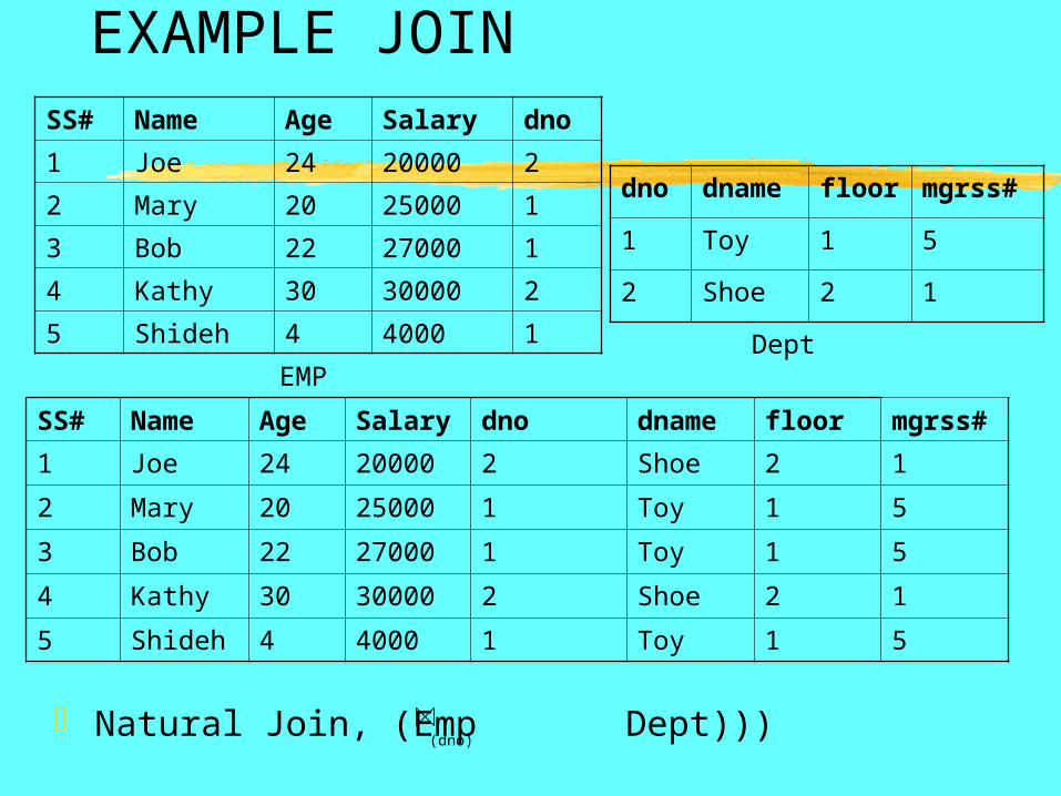
Natural Join, (Emp Dept)))

SS# Name Age Salary dno

1 Joe 24 20000 2

2 Mary 20 25000 1

3 Bob 22 27000 1

4 Kathy 30 30000 2

5 Shideh 4 4000 1

EMP

dno dname

floor mgrss#

1 Toy 1 5

2 Shoe 2 1

Dept

(dno)

SS# Name Age Salary dno dname floor mgrss#

1 Joe 24 20000 2 Shoe 2 1

2 Mary 20 25000 1 Toy 1 5

3 Bob 22 27000 1 Toy 1 5

4 Kathy 30 30000 2 Shoe 2 1

5 Shideh 4 4000 1 Toy 1 5

EXAMPLE JOIN

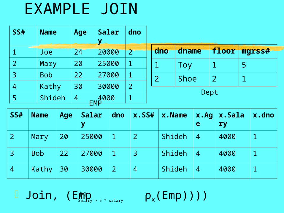
Join, (Emp ρx(Emp))))

SS# Name Age Salary

dno

1 Joe 24 20000 2

2 Mary 20 25000 1

3 Bob 22 27000 1

4 Kathy 30 30000 2

5 Shideh 4 4000 1EMP

dno dname

floor mgrss#

1 Toy 1 5

2 Shoe 2 1Dept

Salary > 5 * salary

SS#

Name

Age Salary

dno x.SS#

x.Name

x.Age

x.Salary

x.dno

2 Mary 20 25000 1 2 Shideh 4 4000 1

3 Bob 22 27000 1 3 Shideh 4 4000 1

4 Kathy 30 30000 2 4 Shideh 4 4000 1

EQUALITY JOIN, NATURAL JOIN, JOIN, SEMI-JOIN (Cont…)

Example: retrieve the name of employees who earn more than Joe: ∏name(Emp (sal>x.sal)бname=‘Joe’(ρ x(Emp)))

Semi-Join selects the columns of one relation that joins with another. It is equivalent to a join followed by a projection: Emp (dno)Dept ≡∏SS#, name, age, salary, dno(Emp

Dept)

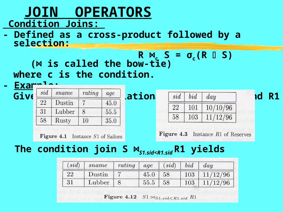
JOIN OPERATORS Condition Joins: - Defined as a cross-product followed by a

selection: R ⋈c S = σc(R S) (⋈ is

called the bow-tie)where c is the condition.

- Example:Given the sample relational instances S1 and R1

The condition join S ⋈S1.sid<R1.sid R1 yields

JOIN OPERATORS Condition Joins: - Defined as a cross-product followed by a

selection: R ⋈c S = σc(R S) (⋈ is

called the bow-tie)where c is the condition.

- Example:Given the sample relational instances S1 and R1

The condition join S ⋈S1.sid<R1.sid R1 yields

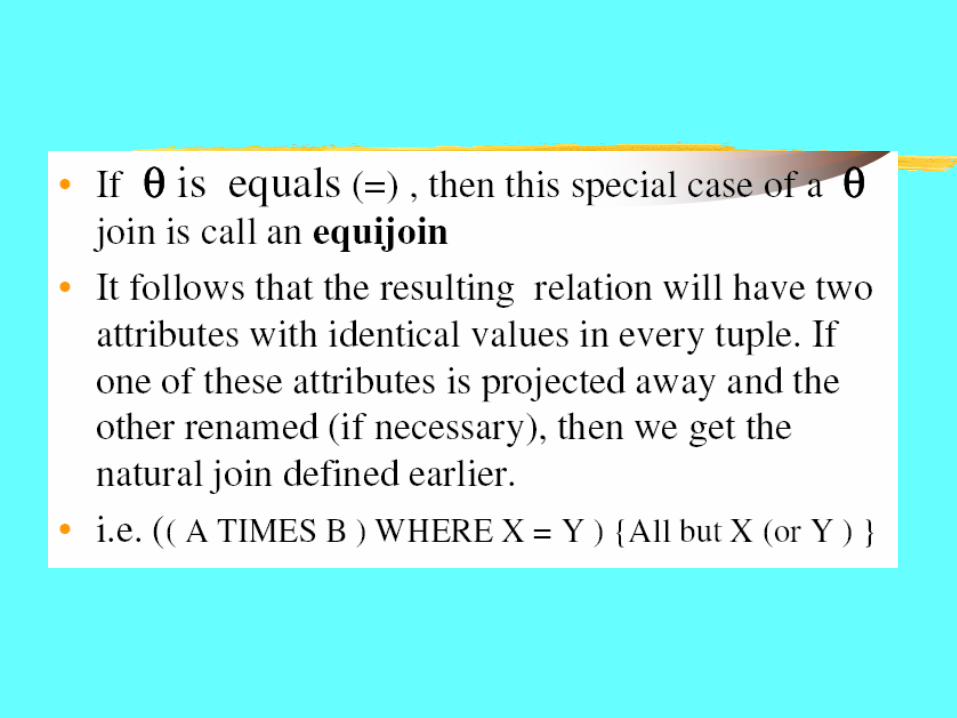
Equijoin:Special case of the condition join where the join condition

consists solely of equalities between two fields in R and S connected by the logical AND operator (∧).

Example: Given the two sample relational instances S1 and R1

The operator S1 R.sid=Ssid R1 yields

Natural Join

- Special case of equijoin where equalities are implicitly specified on all fields having the same name in R and S.

- The condition c is now left out, so that the “bow tie” operator by itself signifies a natural join.

- N. B. If the two relations have no attributes in common, the natural join is simply the cross-product.

Computer 1st ProjectShow how to place            non-attacking queens on a triangular board of side n. Show that this is the maximum possible number of queens.

                 

Tree search example

You need to use

(1) Depth First Search

(2) Backtracking Algorithm

Due Date: Feb. 12, Input, Output format

Feb. 19 Depth first search

Feb. 26 Complete the project.

Tree search example

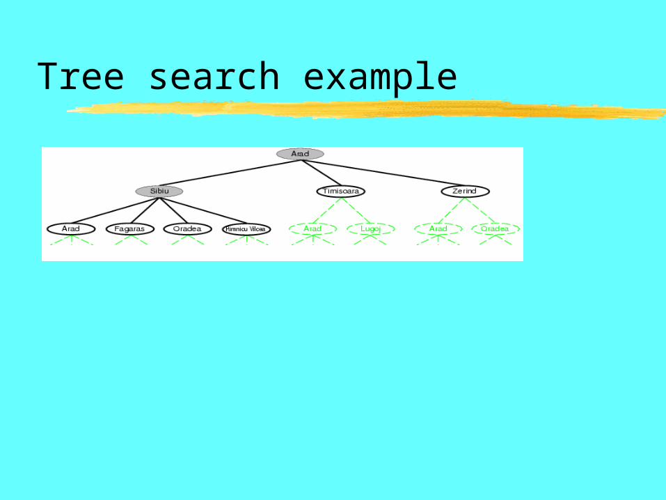
Tree search example

Implementation: general tree search

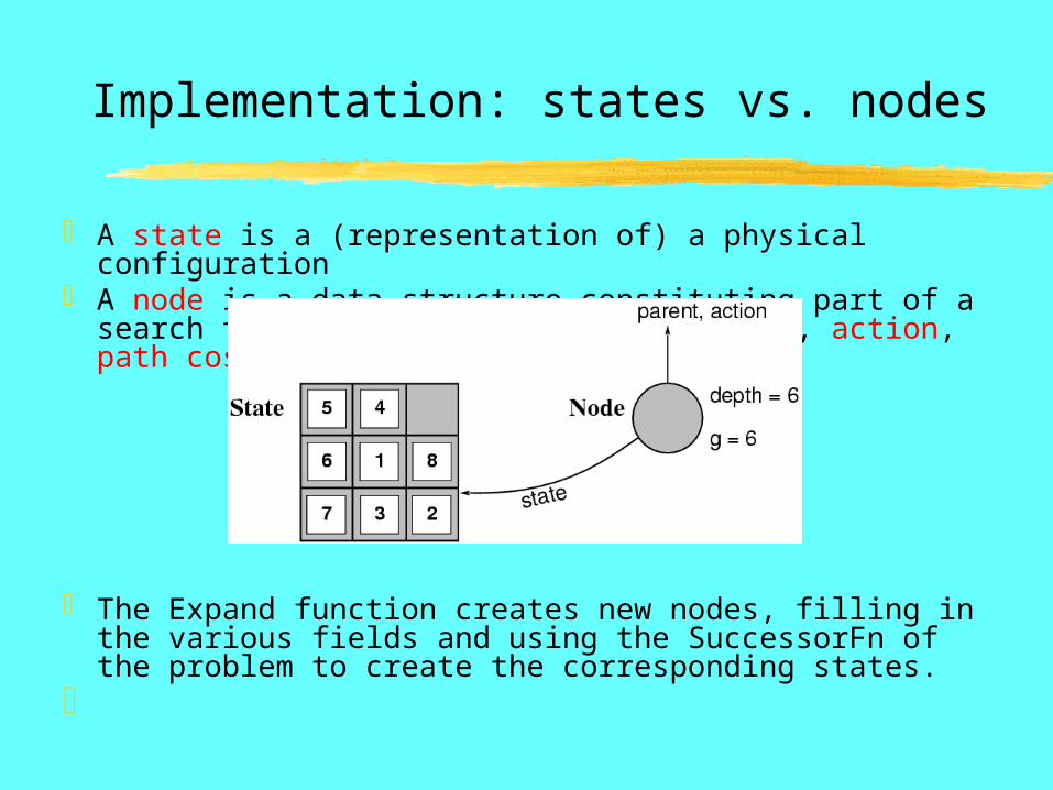
Implementation: states vs. nodes

A state is a (representation of) a physical configuration A node is a data structure constituting part of a search

tree includes state, parent node, action, path cost g(x), depth

The Expand function creates new nodes, filling in the various fields and using the SuccessorFn of the problem to create the corresponding states.

Search strategies

A search strategy is defined by picking the order of node expansion

Strategies are evaluated along the following dimensions: completeness: does it always find a solution if one exists? time complexity: number of nodes generated space complexity: maximum number of nodes in memory optimality: does it always find a least-cost solution?

Time and space complexity are measured in terms of b: maximum branching factor of the search tree d: depth of the least-cost solution m: maximum depth of the state space (may be ∞)

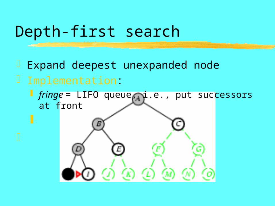
Depth-first search

Expand deepest unexpanded nodeImplementation:

fringe = LIFO queue, i.e., put successors at front

Depth-first search

Expand deepest unexpanded nodeImplementation:

fringe = LIFO queue, i.e., put successors at front

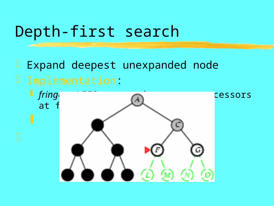
Depth-first search

Expand deepest unexpanded nodeImplementation:

fringe = LIFO queue, i.e., put successors at front

Depth-first search

Expand deepest unexpanded nodeImplementation:

fringe = LIFO queue, i.e., put successors at front

Depth-first search

Expand deepest unexpanded nodeImplementation:

fringe = LIFO queue, i.e., put successors at front

Depth-first search

Expand deepest unexpanded nodeImplementation:

fringe = LIFO queue, i.e., put successors at front

Depth-first search

Expand deepest unexpanded nodeImplementation:

fringe = LIFO queue, i.e., put successors at front

Depth-first search

Expand deepest unexpanded nodeImplementation:

fringe = LIFO queue, i.e., put successors at front

Depth-first search

Expand deepest unexpanded nodeImplementation:

fringe = LIFO queue, i.e., put successors at front

Depth-first search

Expand deepest unexpanded nodeImplementation:

fringe = LIFO queue, i.e., put successors at front

Depth-first search

Expand deepest unexpanded nodeImplementation:

fringe = LIFO queue, i.e., put successors at front

Depth-first search

Expand deepest unexpanded nodeImplementation:

fringe = LIFO queue, i.e., put successors at front

Properties of depth-first search

Complete? No: fails in infinite-depth spaces, spaces with loops Modify to avoid repeated states along path

complete in finite spaces

Time? O(bm): terrible if m is much larger than d but if solutions are dense, may be much faster

than breadth-first

Space? O(bm), i.e., linear space!Optimal? No

Depth-limited search

= depth-first search with depth limit l,i.e., nodes at depth l have no successors

Recursive implementation:

Backtracking Suppose you have to make a series of

decisions, among various choices, where You don’t have enough information to know

what to choose Each decision leads to a new set of choices Some sequence of choices (possibly more

than one) may be a solution to your problem

Backtracking is a methodical way of trying out various sequences of decisions, until you find one that “works”

Backtracking (animation)

start ?

?dead end

dead end

??

dead end

dead end

?

success!

dead end

Terminology I

There are three kinds of nodes:

A tree is composed of nodes

The (one) root node

Internal nodes

Leaf nodes

Backtracking can be thought of as searching a tree for a particular “goal” leaf node

Terminology II

Each non-leaf node in a tree is a parent of one or more other nodes (its children)

Each node in the tree, other than the root, has exactly one parent

parent

children

parent

children

Usually, however, we draw our trees downward, with the root at the top

Real and virtual trees

There is a type of data structure called a tree But we are not using it here

If we diagram the sequence of choices we make, the diagram looks like a tree In fact, we did just this a couple of slides

ago Our backtracking algorithm “sweeps out a

tree” in “problem space”

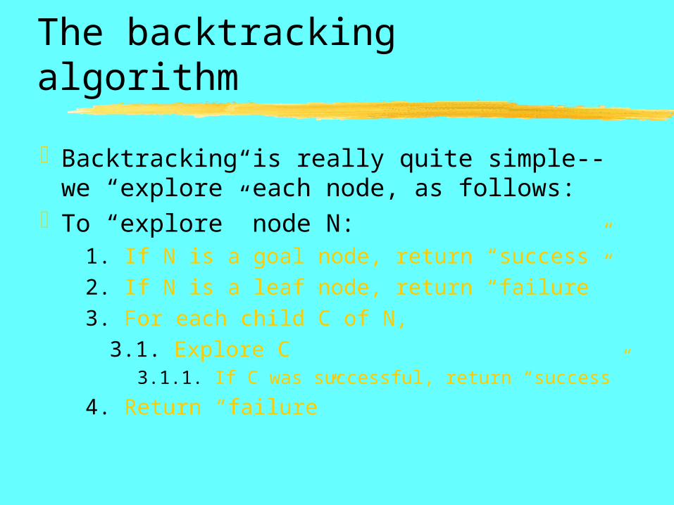
The backtracking algorithm

Backtracking is really quite simple--we “explore” each node, as follows:

To “explore” node N: 1. If N is a goal node, return “success” 2. If N is a leaf node, return “failure” 3. For each child C of N,

3.1. Explore C 3.1.1. If C was successful, return “success”

4. Return “failure”