Greedy Algorithms

Prof. Sin-Min Lee

Department of Computer Science

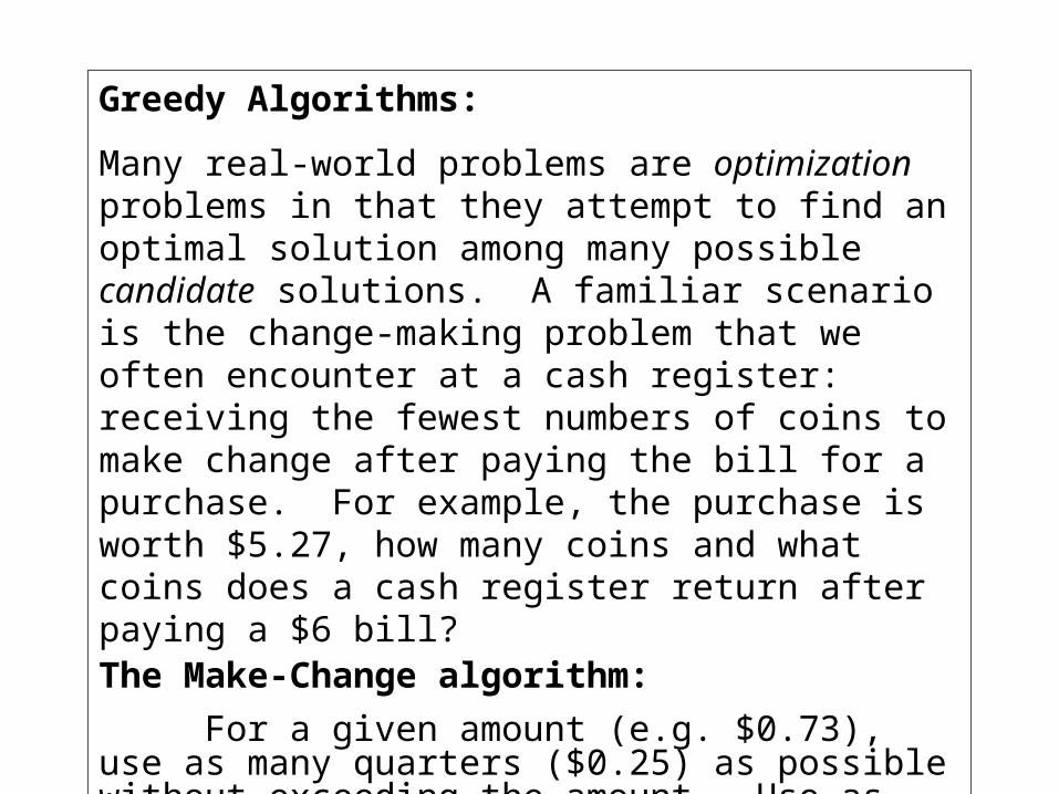
Greedy Algorithms:

Many real-world problems are optimization problems in that they attempt to find an optimal solution among many possible candidate solutions. A familiar scenario is the change-making problem that we often encounter at a cash register: receiving the fewest numbers of coins to make change after paying the bill for a purchase. For example, the purchase is worth $5.27, how many coins and what coins does a cash register return after paying a $6 bill?The Make-Change algorithm:

For a given amount (e.g. $0.73), use as many quarters ($0.25) as possible without exceeding the amount. Use as many dimes ($.10) for the remainder, then use as many nickels ($.05) as possible. Finally, use the pennies ($.01) for the rest.

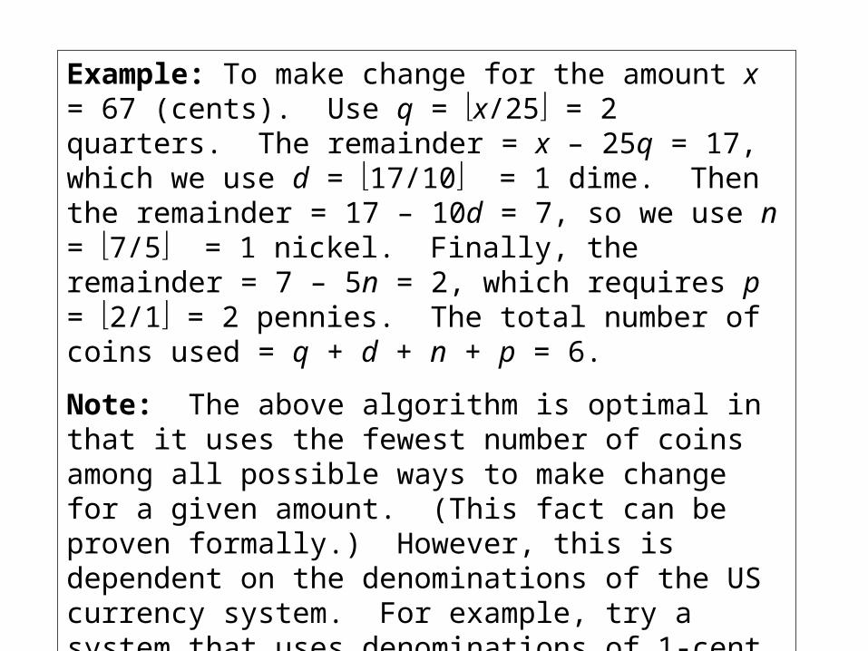
Example: To make change for the amount x = 67 (cents). Use q = x/25 = 2 quarters. The remainder = x – 25q = 17, which we use d = 17/10 = 1 dime. Then the remainder = 17 – 10d = 7, so we use n = 7/5 = 1 nickel. Finally, the remainder = 7 – 5n = 2, which requires p = 2/1 = 2 pennies. The total number of coins used = q + d + n + p = 6.

Note: The above algorithm is optimal in that it uses the fewest number of coins among all possible ways to make change for a given amount. (This fact can be proven formally.) However, this is dependent on the denominations of the US currency system. For example, try a system that uses denominations of 1-cent, 6-cent, and 7-cent coins, and try to make change for x = 18 cents. The greedy strategy uses 2 7-cents and 4 1-cents, for a total of 6 coins. However, the optimal solution is to use 3 6-cent coins.

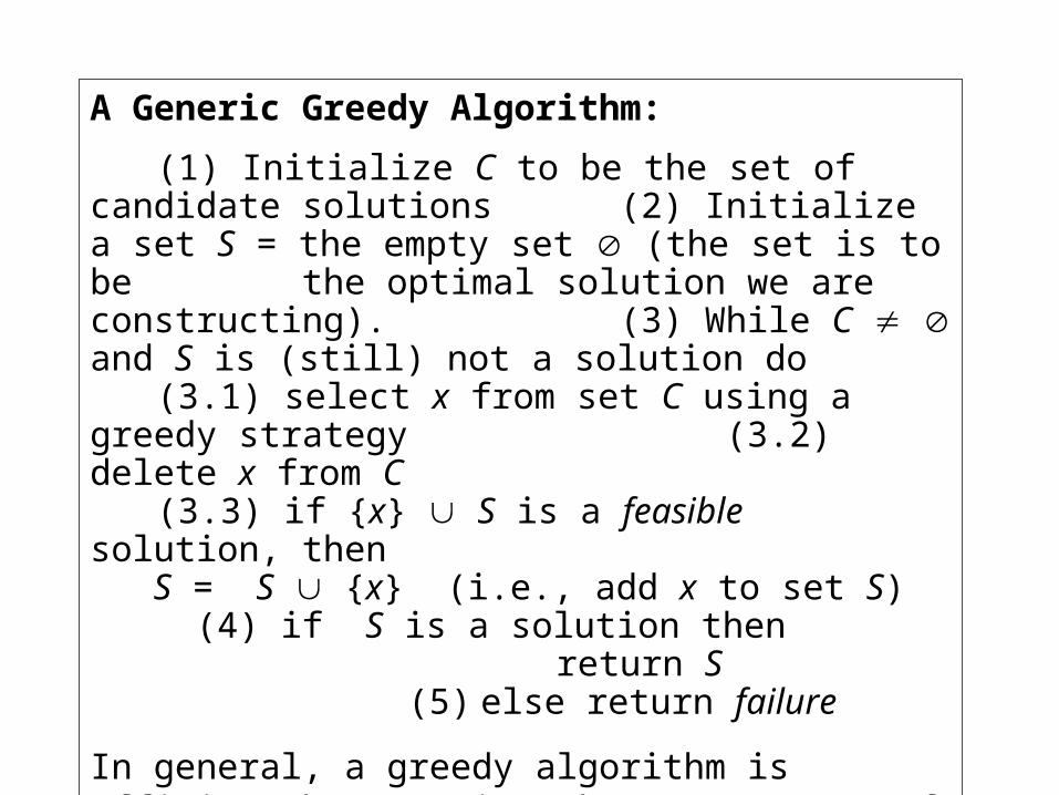
A Generic Greedy Algorithm:

(1) Initialize C to be the set of candidate solutions(2) Initialize a set S = the empty set (the set is to be

the optimal solution we are constructing).(3) While C and S is (still) not a solution do

(3.1) select x from set C using a greedy strategy(3.2) delete x from C(3.3) if {x} S is a feasible solution, then

S = S {x} (i.e., add x to set S)(4) if S is a solution then

return S(5) else return failure

In general, a greedy algorithm is efficient because it makes a sequence of (local) decisions and never backtracks. The solution is not always optimal, however.

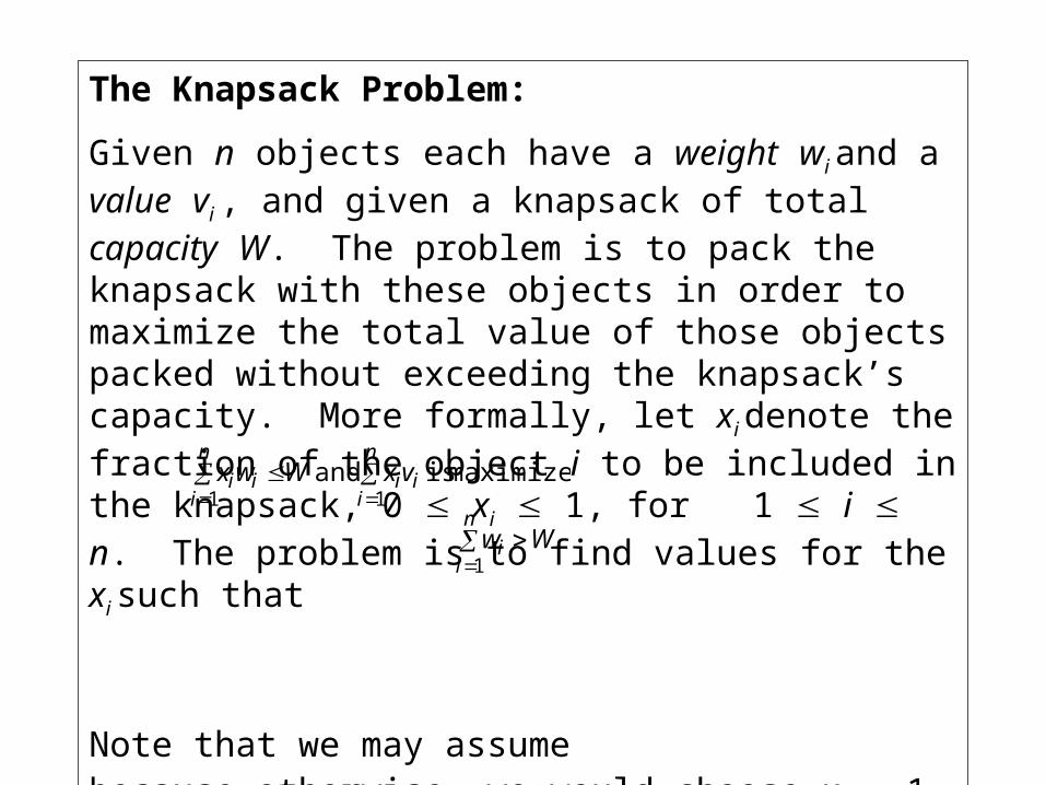
The Knapsack Problem:

Given n objects each have a weight wi and a value vi , and given a knapsack of total capacity W. The problem is to pack the knapsack with these objects in order to maximize the total value of those objects packed without exceeding the knapsack’s capacity. More formally, let xi denote the fraction of the object i to be included in the knapsack, 0 xi 1, for 1 i n. The problem is to find values for the xi such that

Note that we may assume because otherwise, we would choose xi = 1 for each i which would be an obvious

optimal solution.

n

iii

n

iii vxWwx

11maximized. is and

n

ii Ww

1

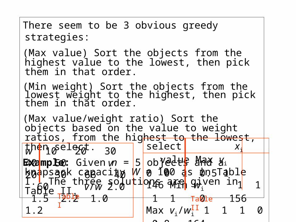
There seem to be 3 obvious greedy strategies:

(Max value) Sort the objects from the highest value to the lowest, then pick them in that order.

(Min weight) Sort the objects from the lowest weight to the highest, then pick them in that order.

(Max value/weight ratio) Sort the objects based on the value to weight ratios, from the highest to the lowest, then select.

Example: Given n = 5 objects and a knapsack capacity W = 100 as in Table I. The three solutions are given in Table II.

w 10 20 30 40 50 v 20 30 66 40 60 v/w 2.0 1.5 2.2 1.0 1.2

Table I

select xi value Max vi 0 0 1 0.5 1 146 Min wi 1 1 1 1 0 156 Max vi/wi 1 1 1 0 0.8 164

Table II

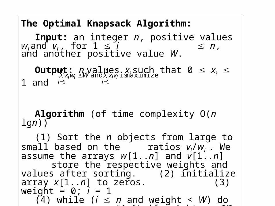
The Optimal Knapsack Algorithm:

Input: an integer n, positive values wi and vi , for 1 i n, and another positive value W.

Output: n values xi such that 0 xi 1 and

Algorithm (of time complexity O(n lgn))

(1) Sort the n objects from large to small based on the ratios vi/wi . We assume the arrays w[1..n] and v[1..n] store the respective weights and values after sorting.(2) initialize array x[1..n] to zeros.(3) weight = 0; i = 1(4) while (i n and weight < W) do

(4.1) if weight + w[i] W then x[i] = 1 (4.2) else x[i] = (W – weight) / w[i] (4.3) weight = weight + x[i] * w[i] (4.4) i++

n

iii

n

iii vxWwx

11maximized. is and

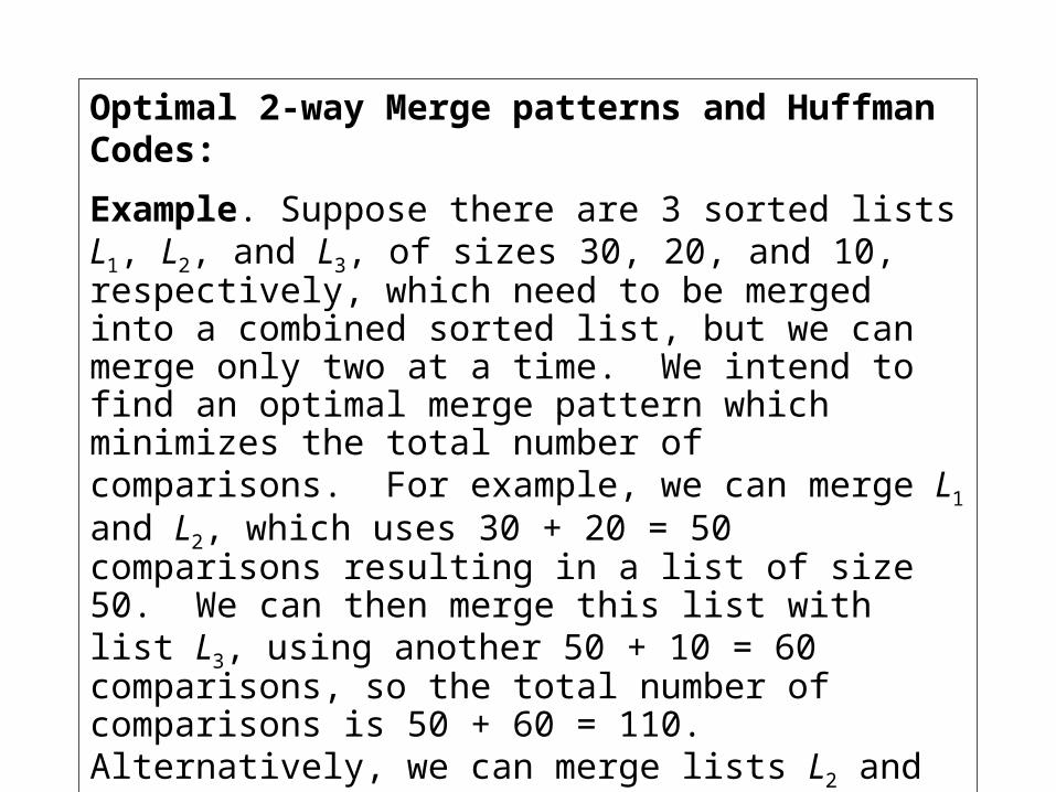
Optimal 2-way Merge patterns and Huffman Codes:

Example. Suppose there are 3 sorted lists L1, L2, and L3, of sizes 30, 20, and 10, respectively, which need to be merged into a combined sorted list, but we can merge only two at a time. We intend to find an optimal merge pattern which minimizes the total number of comparisons. For example, we can merge L1 and L2, which uses 30 + 20 = 50 comparisons resulting in a list of size 50. We can then merge this list with list L3, using another 50 + 10 = 60 comparisons, so the total number of comparisons is 50 + 60 = 110. Alternatively, we can merge lists L2 and L3, using 20 + 10 = 30 comparisons, the resulting list (size 30) can then be merged with list L1, for another 30 + 30 = 60 comparisons. So the total number of comparisons is 30 + 60 = 90. It doesn’t take long to see that this latter merge pattern is the optimal one.

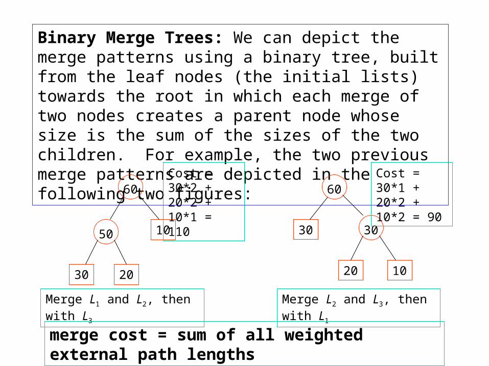
Binary Merge Trees: We can depict the merge patterns using a binary tree, built from the leaf nodes (the initial lists) towards the root in which each merge of two nodes creates a parent node whose size is the sum of the sizes of the two children. For example, the two previous merge patterns are depicted in the following two figures:

Merge L1 and L2, then with L3

30 20

50 10

60

1020

30 30

60

Merge L2 and L3, then with L1

merge cost = sum of all weighted external path lengths

Cost = 30*2 + 20*2 + 10*1 = 110

Cost = 30*1 + 20*2 + 10*2 = 90

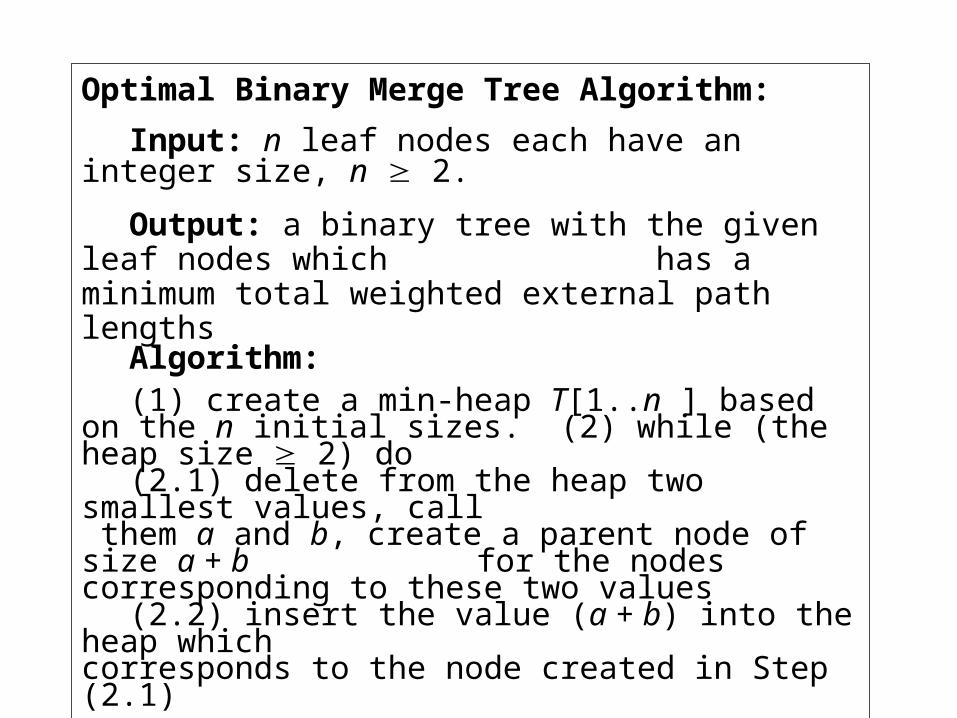
Optimal Binary Merge Tree Algorithm:

Input: n leaf nodes each have an integer size, n 2.

Output: a binary tree with the given leaf nodes which has a minimum total weighted external path lengths

Algorithm:(1) create a min-heap T[1..n ] based on the n initial sizes.(2) while (the heap size 2) do

(2.1) delete from the heap two smallest values, call them a and b, create a parent node of size a + b

for the nodes corresponding to these two values(2.2) insert the value (a + b) into the heap which

corresponds to the node created in Step (2.1)

When the algorithm terminates, there is a single value left in the heap whose corresponding node is the root of the optimal binary merge tree. The algorithm’s time complexity is O(n lgn) because Step (1) takes O(n) time; Step (2) runs O(n) iterations, in which each iteration takes O(lgn) time.

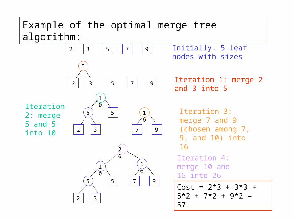
Example of the optimal merge tree algorithm:

2 3 5 7 9

2 3

5

5 7 9

2 3

5 5

10

7 9

Initially, 5 leaf nodes with sizes

Iteration 1: merge 2 and 3 into 5

Iteration 2: merge 5 and 5 into 10

16 Iteration 3: merge 7 and 9 (chosen among 7, 9, and 10) into 16

2 3

5

10

5 7 9

16

26

Iteration 4: merge 10 and 16 into 26

Cost = 2*3 + 3*3 + 5*2 + 7*2 + 9*2 = 57.

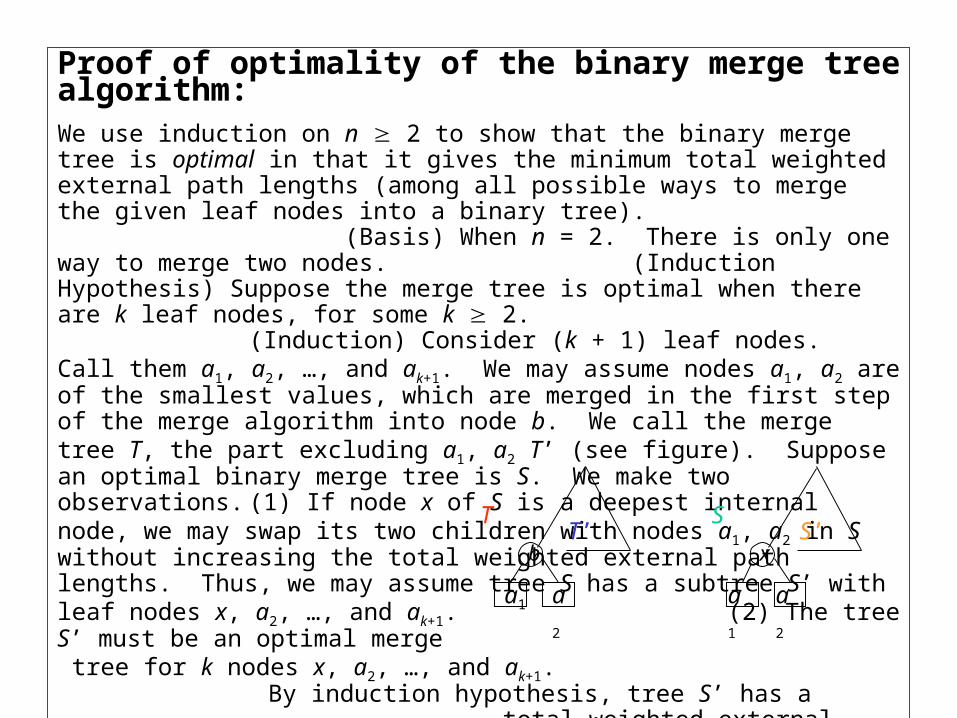
Proof of optimality of the binary merge tree algorithm:We use induction on n 2 to show that the binary merge tree is optimal in that it gives the minimum total weighted external path lengths (among all possible ways to merge the given leaf nodes into a binary tree).

(Basis) When n = 2. There is only one way to merge two nodes.(Induction Hypothesis) Suppose the merge tree is optimal when there are k leaf

nodes, for some k 2.(Induction) Consider (k + 1) leaf nodes. Call them a1, a2, …, and ak+1. We may

assume nodes a1, a2 are of the smallest values, which are merged in the first step of the merge algorithm into node b. We call the merge tree T, the part excluding a1, a2 T’ (see figure). Suppose an optimal binary merge tree is S. We make two observations.

(1) If node x of S is a deepest internal node, we may swap its two children with nodes a1, a2 in S without increasing the total weighted external path lengths. Thus, we may assume tree S has a subtree S’ with leaf nodes x, a2, …, and ak+1.

(2) The tree S’ must be an optimal merge tree for k nodes x, a2, …, and ak+1. By induction hypothesis, tree S’ has a total weighted external path lengths equal to that of tree T’. Therefore, the total weighted external path lengths of T equals to that of tree S, proving the optimality of T.

TT’

SS’

x

a1 a2 a1 a2

b

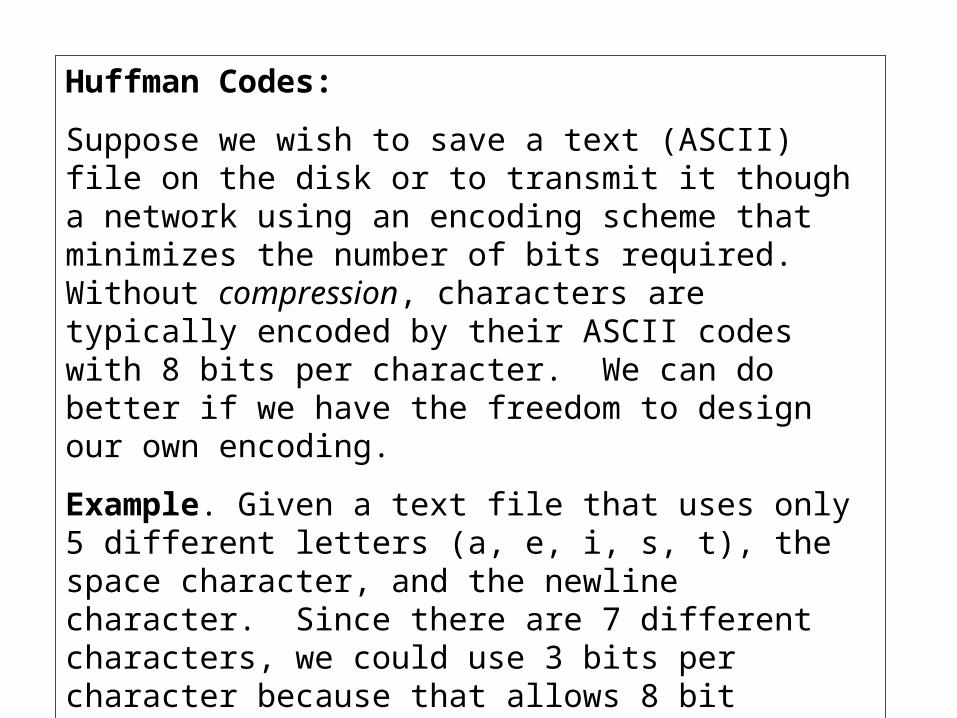
Huffman Codes:

Suppose we wish to save a text (ASCII) file on the disk or to transmit it though a network using an encoding scheme that minimizes the number of bits required. Without compression, characters are typically encoded by their ASCII codes with 8 bits per character. We can do better if we have the freedom to design our own encoding.

Example. Given a text file that uses only 5 different letters (a, e, i, s, t), the space character, and the newline character. Since there are 7 different characters, we could use 3 bits per character because that allows 8 bit patterns ranging from 000 through 111 (so we still one pattern to spare). The following table shows the encoding of characters, their frequencies, and the size of encoded (compressed) file.

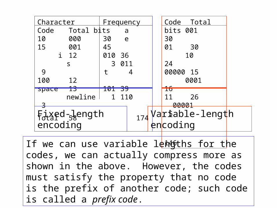
Character Frequency Code Total bits a 10 000 30 e 15 001 45 i 12 010 36 s 3 011 9 t 4 100 12 space 13 101 39 newline 1 110 3

Total 58 174

Code Total bits 001 30 01 30 10 24 00000 15 0001 16 11 26 00001 5

146

Fixed-length encoding Variable-length encoding

If we can use variable lengths for the codes, we can actually compress more as shown in the above. However, the codes must satisfy the property that no code is the prefix of another code; such code is called a prefix code.

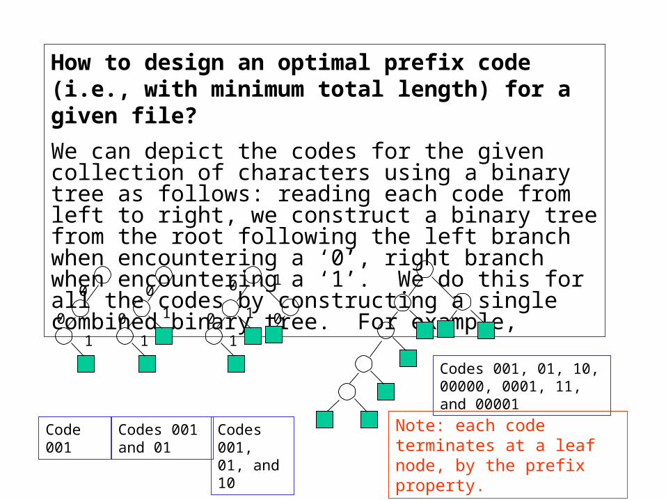
How to design an optimal prefix code (i.e., with minimum total length) for a given file?

We can depict the codes for the given collection of characters using a binary tree as follows: reading each code from left to right, we construct a binary tree from the root following the left branch when encountering a ‘0’, right branch when encountering a ‘1’. We do this for all the codes by constructing a single combined binary tree. For example,

Code 001 Codes 001 and 01

Codes 001, 01, and 10

Codes 001, 01, 10, 00000, 0001, 11, and 00001

0

0

1

0

0 1

1

1

0

0

10

1

Note: each code terminates at a leaf node, by the prefix property.

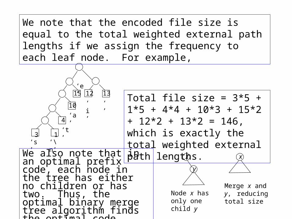
We note that the encoded file size is equal to the total weighted external path lengths if we assign the frequency to each leaf node. For example,

3‘s’

1‘\n’

4

‘t’

10

‘a’

15‘e’

12

‘i’

13

‘ ’Total file size = 3*5 + 1*5 + 4*4 + 10*3 + 15*2 + 12*2 + 13*2 = 146, which is exactly the total weighted external path lengths.

We also note that in an optimal prefix code, each node in the tree has either no children or has two. Thus, the optimal binary merge tree algorithm finds the optimal code (Huffman code). Node x has only

one child y

x

y

x

Merge x and y, reducing total size

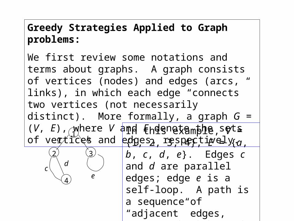
Greedy Strategies Applied to Graph problems:

We first review some notations and terms about graphs. A graph consists of vertices (nodes) and edges (arcs, links), in which each edge “connects” two vertices (not necessarily distinct). More formally, a graph G = (V, E), where V and E denote the sets of vertices and edges, respectively.

1

2 3

4

a b

cd

e

In this example, V = {1, 2, 3, 4}, E = {a, b, c, d, e}. Edges c and d are parallel edges; edge e is a self-loop. A path is a sequence of “adjacent” edges, e.g., path abeb, path acdab.

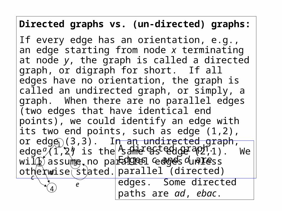
Directed graphs vs. (un-directed) graphs:

If every edge has an orientation, e.g., an edge starting from node x terminating at node y, the graph is called a directed graph, or digraph for short. If all edges have no orientation, the graph is called an undirected graph, or simply, a graph. When there are no parallel edges (two edges that have identical end points), we could identify an edge with its two end points, such as edge (1,2), or edge (3,3). In an undirected graph, edge (1,2) is the same as edge (2,1). We will assume no parallel edges unless otherwise stated.

1

2 3

e

a b

cd

A directed graph. Edges c and d are parallel (directed) edges. Some directed paths are ad, ebac.

4

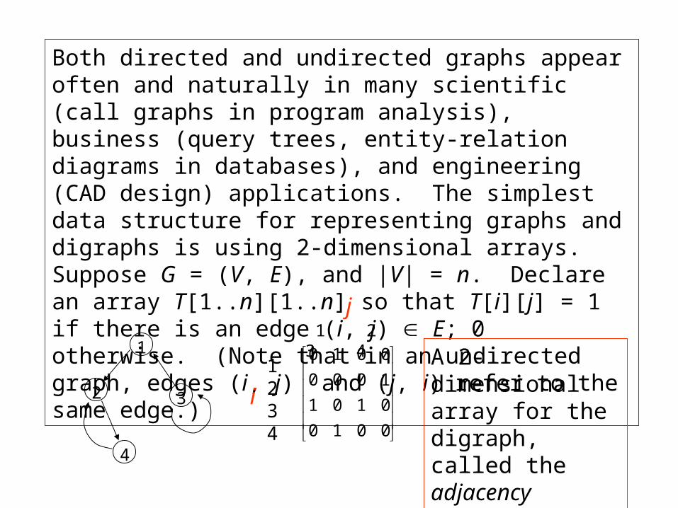
Both directed and undirected graphs appear often and naturally in many scientific (call graphs in program analysis), business (query trees, entity-relation diagrams in databases), and engineering (CAD design) applications. The simplest data structure for representing graphs and digraphs is using 2-dimensional arrays. Suppose G = (V, E), and |V| = n. Declare an array T[1..n][1..n] so that T[i][j] = 1 if there is an edge (i, j) E; 0 otherwise. (Note that in an undirected graph, edges (i, j) and (j, i) refer to the same edge.)

1

4

2 3

0010

0101

1000

0010

1 2 3 4

1234

A 2-dimensional array for the digraph, called the adjacency matrix.

i

j

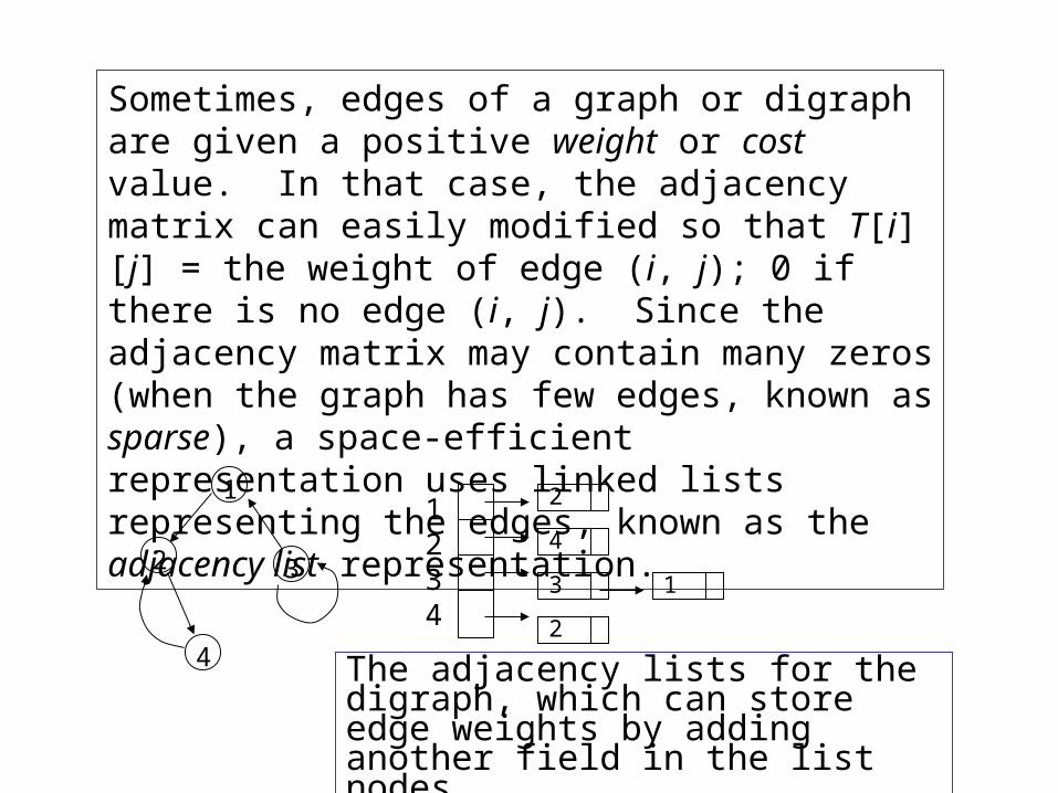
Sometimes, edges of a graph or digraph are given a positive weight or cost value. In that case, the adjacency matrix can easily modified so that T[i][j] = the weight of edge (i, j); 0 if there is no edge (i, j). Since the adjacency matrix may contain many zeros (when the graph has few edges, known as sparse), a space-efficient representation uses linked lists representing the edges, known as the adjacency list representation.

1

4

2 3

1234

2

4

3 1

2

The adjacency lists for the digraph, which can store edge weights by adding another field in the list nodes.

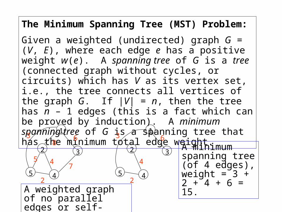
The Minimum Spanning Tree (MST) Problem:

Given a weighted (undirected) graph G = (V, E), where each edge e has a positive weight w(e). A spanning tree of G is a tree (connected graph without cycles, or circuits) which has V as its vertex set, i.e., the tree connects all vertices of the graph G. If |V| = n, then the tree has n – 1 edges (this is a fact which can be proved by induction). A minimum spanning tree of G is a spanning tree that has the minimum total edge weight.

1

4

2 3

5

A weighted graph of no parallel edges or self-loops

38

6

5 4

2

745

3

4

2

1

2 3

6A minimum spanning tree (of 4 edges), weight = 3 + 2 + 4 + 6 = 15.

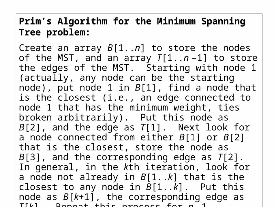
Prim’s Algorithm for the Minimum Spanning Tree problem:

Create an array B[1..n] to store the nodes of the MST, and an array T[1..n –1] to store the edges of the MST. Starting with node 1 (actually, any node can be the starting node), put node 1 in B[1], find a node that is the closest (i.e., an edge connected to node 1 that has the minimum weight, ties broken arbitrarily). Put this node as B[2], and the edge as T[1]. Next look for a node connected from either B[1] or B[2] that is the closest, store the node as B[3], and the corresponding edge as T[2]. In general, in the kth iteration, look for a node not already in B[1..k] that is the closest to any node in B[1..k]. Put this node as B[k+1], the corresponding edge as T[k]. Repeat this process for n –1 iterations (k = 1 to n –1). This is a greedy strategy because in each iteration, the algorithm looks for the minimum weight edge to include next while maintaining the tree property (i.e., avoiding cycles). At the end there are exactly n –1 edges without cycles, which must be a spanning tree.

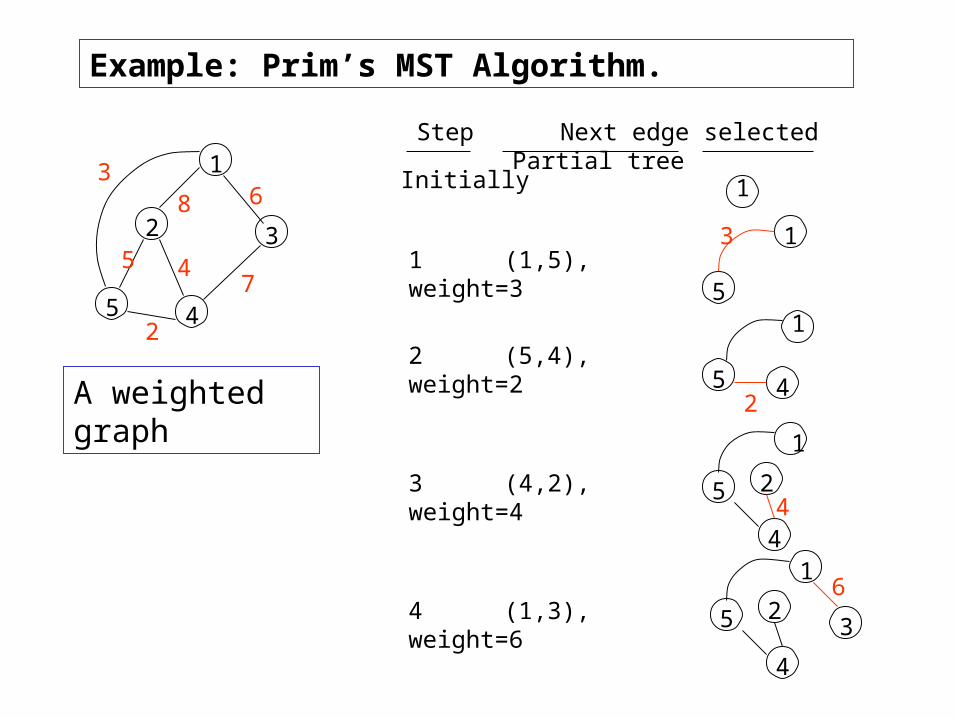
Example: Prim’s MST Algorithm.

5

5 4

2

74

2 3

138 6

A weighted graph

Step Next edge selected Partial tree

Initially 1

1 (1,5), weight=35

1

2 (5,4), weight=21

5 4

3 (4,2), weight=4 5

4

2

1

4 (1,3), weight=6 2

1

35

4

3

2

4

6

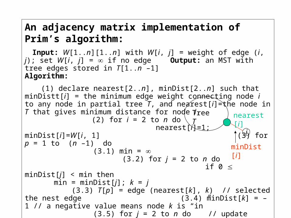
An adjacency matrix implementation of Prim’s algorithm:Input: W[1..n][1..n] with W[i, j] = weight of edge (i, j); set W[i, j] = if no edgeOutput: an MST with tree edges stored in T[1..n –1]Algorithm:

(1) declare nearest[2..n], minDist[2..n] such that minDistt[i] = the minimum edge weight connecting node i to any node in partial tree T, and nearest[i]=the node in T that gives minimum distance for node i.

(2) for i = 2 to n do nearest[i]=1; minDist[i]=W[i, 1] (3) for p = 1 to (n –1) do

(3.1) min = (3.2) for j = 2 to n do

if 0 minDist[j] < min thenmin = minDist[j]; k = j

(3.3) T[p] = edge (nearest[k], k) // selected the nest edge (3.4) minDist[k] = –1 // a negative value means node k is “in” (3.5) for j = 2 to n do // update minDist and nearest values

if W[j, k] < minDist[j] thenminDist[j] = W[j, k]; nearest[j] = k

The time complexity is O(n2) because Step (3) runs O(n) iterations, each iteration runs O(n) time in Steps (3.2) and (3.5).

Tree T

i

nearest[i]

minDist[i]

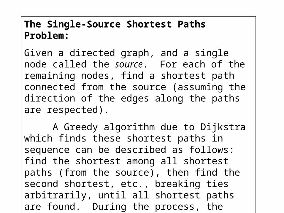
The Single-Source Shortest Paths Problem:

Given a directed graph, and a single node called the source. For each of the remaining nodes, find a shortest path connected from the source (assuming the direction of the edges along the paths are respected).

A Greedy algorithm due to Dijkstra which finds these shortest paths in sequence can be described as follows: find the shortest among all shortest paths (from the source), then find the second shortest, etc., breaking ties arbitrarily, until all shortest paths are found. During the process, the collection of all the shortest paths determined so far form a tree; the next shortest path is selected by finding a node that is one edge away from the current tree and has the shortest distance measured from the source.

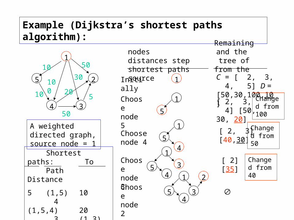
Example (Dijkstra’s shortest paths algorithm):

1

2

34

5

A weighted directed graph, source node = 1

10 50

100

10

30

20

50

5

Remaining nodes and the distances

step tree of shortest paths from the source

Initially 1 C = [ 2, 3, 4, 5] D = [50,30,100,10]

Choose node 5

1

5[ 2, 3, 4] [50,30, 20]

Changed from 100

Choose node 4

1

54

[ 2, 3] [40,30]

Changed from 50

Choose node 3 5

4

1

3[ 2] [35]

Changed from 40

Choose node 2 3

1

54

2

Shortest paths: To Path Distance

5 (1,5) 10 4 (1,5,4) 20 3 (1,3) 30 2 (1,3,2) 35

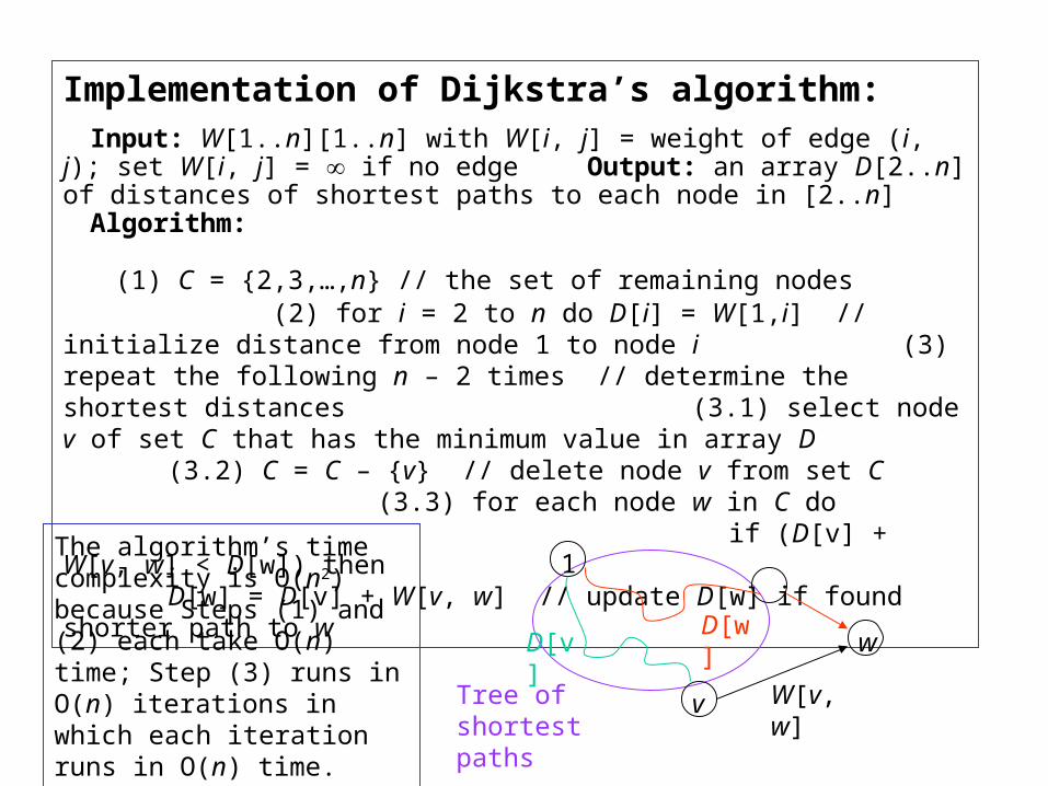
Implementation of Dijkstra’s algorithm:Input: W[1..n][1..n] with W[i, j] = weight of edge (i, j); set W[i, j] = if no edgeOutput: an array D[2..n] of distances of shortest paths to each node in [2..n]Algorithm:

(1) C = {2,3,…,n} // the set of remaining nodes (2) for i = 2 to n do D[i] = W[1,i] // initialize distance from node 1 to node i

(3) repeat the following n – 2 times // determine the shortest distances(3.1) select node v of set C that has the minimum value in array D(3.2) C = C – {v} // delete node v from set C(3.3) for each node w in C do if (D[v] + W[v, w] < D[w]) then

D[w] = D[v] + W[v, w] // update D[w] if found shorter path to w

1

v

w

W[v,w]

D[v]D[w]

Tree of shortest paths

The algorithm’s time complexity is O(n2) because Steps (1) and (2) each take O(n) time; Step (3) runs in O(n) iterations in which each iteration runs in O(n) time.

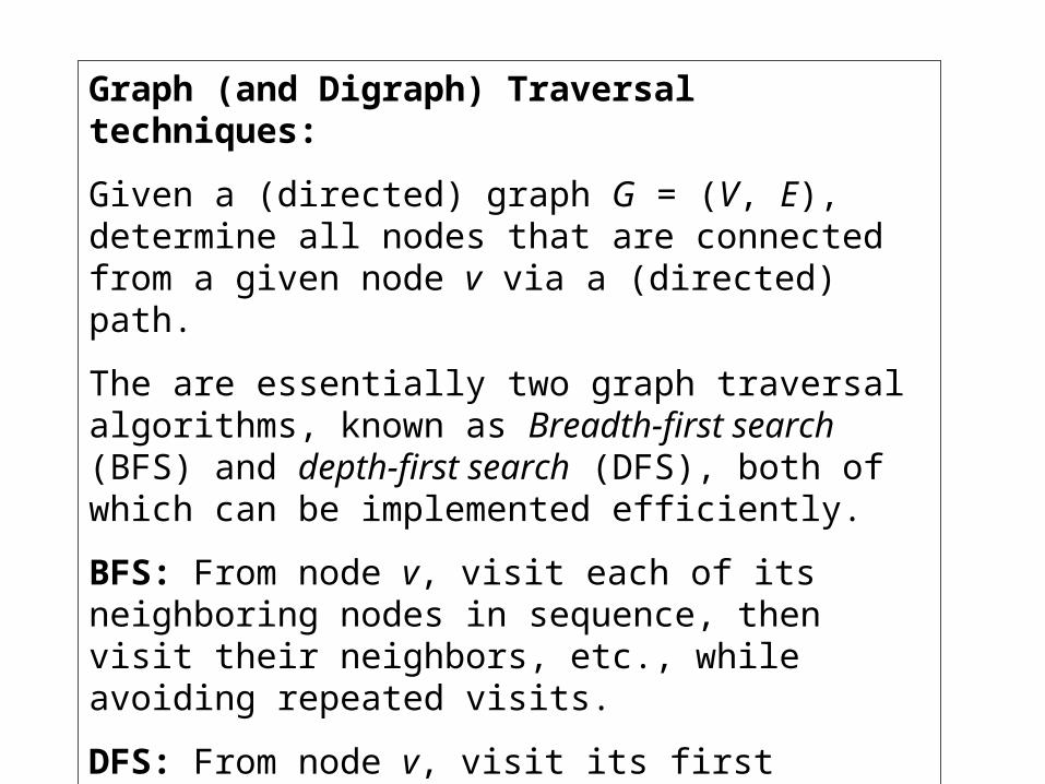
Graph (and Digraph) Traversal techniques:

Given a (directed) graph G = (V, E), determine all nodes that are connected from a given node v via a (directed) path.

The are essentially two graph traversal algorithms, known as Breadth-first search (BFS) and depth-first search (DFS), both of which can be implemented efficiently.

BFS: From node v, visit each of its neighboring nodes in sequence, then visit their neighbors, etc., while avoiding repeated visits.

DFS: From node v, visit its first neighboring node and all its neighbors using recursion, then visit node v’s second neighbor applying the same procedure, until all v’s neighbors are visited, while avoiding repeated visits.

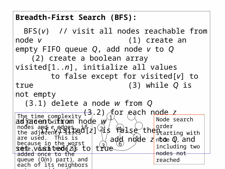
Breadth-First Search (BFS):

BFS(v) // visit all nodes reachable from node v (1) create an empty FIFO queue Q, add node v to Q

(2) create a boolean array visited[1..n], initialize all values to false except for visited[v] to true(3) while Q is not empty (3.1) delete a node w from Q (3.2) for each node z adjacent from node w

if visited[z] is false then add node z to Q and set visited[z] to true

1

2 4

35

6

Node search order starting with node 1, including two nodes not reached

The time complexity is O(n+e) with n nodes and e edges, if the adjacency lists are used. This is because in the worst case, each node is added once to the queue (O(n) part), and each of its neighbors gets considered once (O(e) part).

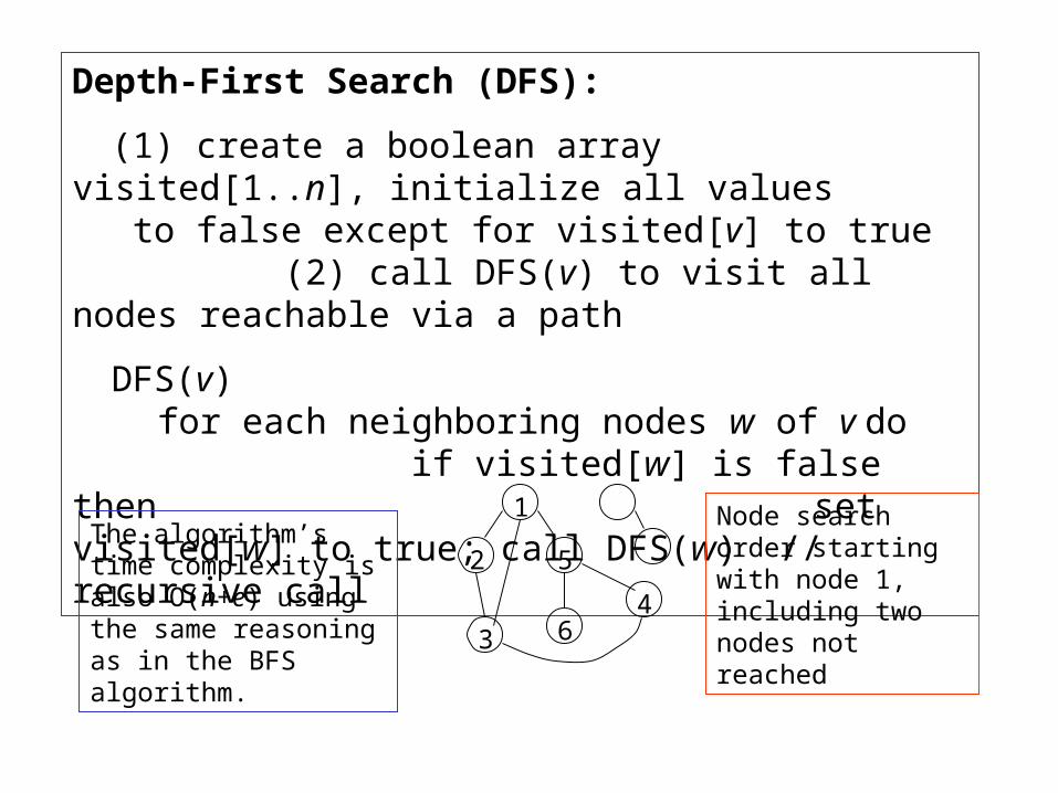
Depth-First Search (DFS):

(1) create a boolean array visited[1..n], initialize all values to false except for visited[v] to true

(2) call DFS(v) to visit all nodes reachable via a path

DFS(v) for each neighboring nodes w of v do

if visited[w] is false then set visited[w] to true; call DFS(w) // recursive call

1

2 5

3 64

Node search order starting with node 1, including two nodes not reached

The algorithm’s time complexity is also O(n+e) using the same reasoning as in the BFS algorithm.