regression kink with an unknown threshold · pdf filethreshold. a regression kink model ......
TRANSCRIPT
Regression Kink with an Unknown Threshold
Bruce E. Hansen∗
University of Wisconsin†
February 2015
Abstract
This paper explores estimation and inference in a regression kink model with an unknown
threshold. A regression kink model (or continuous threshold model) is a threshold regression con-
strained to be everywhere continuous with a kink at an unknown threshold. We present methods
for estimation, to test for the presence of the threshold, for inference on the regression parameters,
and for inference on the regression function. A novel finding is that inference on the regression
function is non-standard since the regression function is a non-differentiable function of the para-
meters. We apply recently developed methods for inference on non-differentiable functions. The
theory is illustrated by an application to the growth & debt problem introduced by Reinhart and
Rogoff (2010), using their long-span time-series for the United States.
∗Research supported by the National Science Foundation. I thank Zheng Fang, Han Hong, Jessie Li, Tzu-Chi Lin,and Andres Santos for very helpful comments, suggestions, and correspondence which were critical for the results
developed here.†Department of Economics, 1180 Observatory Drive, University of Wisconsin, Madison, WI 53706.
1 Introduction
The regression kink model was popularized by Card, Lee, Pei andWeber (2012) as a modification
of the regression discontinuity model. In the regression kink model, the regression function is
continuous but the slope has a discontinuity at a threshold point, hence a “kink”. This model has
gained much empirical attention, including applications by Landais (2012) and Ganong and Jager
(2014). The traditional regression discontinuity model assumes that the threshold is known, but in
some cases (such as Card, Mas and Rothstein, 2008) it is unknown and must be estimated.
Regression discontinuity models are similar to threshold regression models. The latter were
introduced by Howell Tong (1983, 1990) in the context of nonlinear autoregression, but can be
applied to many nonlinear regression contexts. Most of the literature and methods focus on the
discontinuous (unconstrained) threshold model, where the regression model is split into two (or
more) groups based on a threshold indicator. A notable exception is the continuous threshold
model introduced by Chan and Tsay (1998), which is identical to a regression kink model with
piecewise linear regression segments. One economic application of the continuous threshold model
is Cox, Hansen, and Jimenez (2004). The regression kink model may be appealing for empirical
applications where the threshold effect focuses on one variable and there is no reason to expect a
discontinuous regression response at the threshold.
This paper extends the theory of Chan and Tsay (1998), considering the problems of testing for
a threshold effect, inference on the regression parameters, and inference on the regression function.
As in Chan and Tsay (1998) we confine attention to the context where the regression segments are
linear rather than nonparametric. This is appropriate in contexts of moderate sample sizes where
nonparametric methods may be inappropriate.
There is a large literature on discontinuous threshold regression. For the problem of testing
for a threshold effect, relevant contributions include Chan (1990, 1991), Chan and Tong (1990)
and Hansen (1996). For inference on the regression parameters, relevant papers include Chan
(1993), Hansen (2000), and Seo and Linton (2007). Panel data models have been developed by
Hansen (1999) and Ramirez-Rondan (2013). Instrumental variables estimation by Caner and
Hansen (2004). An estimation and inference theory for regression discontinuity with unknown
thresholds has been developed by Porter and Yu (2014).
For illustration, we apply the regression kink model to the growth & debt problem made famous
by Reinhart and Rogoff (2010). These authors argued that there is a nonlinear effect of aggregate
debt on economic growth, specifically that as the ratio of debt to GDP increases pass some threshold,
aggregate economic growth will tend to slow. This can be formalized as a regression kink problem,
where GDP growth is the dependent variable and the debt/GDP ratio is the key regressor and
threshold variable. Econometric analysis of their proposition using threshold regression tools has
been pursued by several authors, including Caner, Grennes and Koehler (2010), Cecchetti, Mohanty,
and Zampolli (2011), and Lin (2014). These papers investigate the Reinhart-Rogoff proposition
using a variety of cross-section, panel, and time-series regressions, but all have focused on the
discontinuous threshold regression model. We add to this literature by a small investigation using
1
1800 1850 1900 1950 2000
−10
−5
05
1015
year
GD
P G
row
th R
ate
1800 1850 1900 1950 2000
020
4060
8010
012
0
year
Deb
t/GD
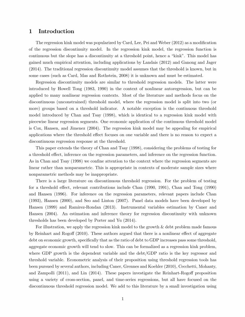
PFigure 1: Annual U.S. Real GDP Growth Rate and GDP/Debt Ratio, 1791-2009
long-span U.S. time-series data.
During our investigation we encounter one novel technical issue. While the parameter estimates
in the regression kink model are asymptotically normal (as shown by Chan and Tsay (1998)),
the estimates of the regression function itself are not asymptotically normal, since the regression
function is a non-differentiable function of the parameter estimates. Consequently conventional
inference methods cannot be applied to the regression function. To address this issue we use recently
developed inference methods by Fang and Santos (2014) and Hong and Li (2015), and present a new
non-normal distribution theory for the regression function estimates, and shown how to construct
numerical delta method bootstrap confidence intervals for the regression function.
Our organization is as follows. Section 2 introduces the model. Section 3 describes least-squares
estimation of the model parameters. Section 4 discusses testing for a threshold effect in the context
of the model. Section 5 presents an asymptotic distribution theory for the parameter estimates and
discusses confidence interval construction. Section 6 discusses inference on the regression function.
A formal proof of Theorem 2 is presented in the Appendix.
The data and R code for the empirical and simulation work reported in the paper is available
on the author’s webpage http://www.ssc.wisc.edu/~bhansen/
2 Model
Our regression kink model takes the form
= 1( − )− + 2( − )+ + 03 + (1)
2
where , and are scalars, and is an -vector which includes an intercept. The variables
( ) are observed for = 1 The parameters are 1, 2, 3 and . We use ()− = min[ 0]and ()+ = max[ 0] to denote the “negative part” and “postive part” of a real number . In model
(1) the slope with respect to the variable equals 1 for values of less than , and equals 2
for values of greater than yet the regression function is continuous in all variables.
The model (1) is a regression kink model because the regression function is continuous in the
variables and , but the slope with respect to is discontinuous (has a kink) at = . The model
(1) specifies the regression segments to be linear, but this could be modified to any parametric form
(such as a polynomial). The conventional regression kink design assumes that the threshold point
is known. Instead, we treat the parameter as an unknown to be estimated.
The model (1) has = 3 + parameters. = (1 2 3) are the regression slopes and are
generally unconstrained so that ∈ R−1. The parameter is called the “threshold”, “knot” or“kink point”. The model (1) only makes sense if the threshold is in the interior of the support
of the threshold variable . We thus assume that ∈ Γ where Γ is compact and strictly in theinterior of the support of
As an empirical example, consider the growth/debt regression problem of Reinhart and Rogoff
(2010). They argued that economic growth tends to slow when the level of government debt relative
to GDP exceeds a threshold. To write this as a regression, we set to be the real GDP growth
rate in year and to the debt to GDP percentage from the previous year (so that it is plausibly
pre-determined). We set = (−1 1)0 so that the regression contains a lagged dependent variableto ensure that the error is approximately serially uncorrelated.
We focus on the United States and use the long span time series for the years 1792-2009 gathered
by Reinhart and Rogoff and posted on their website, so that there are = 218 observations. We
display time-series plots of the two series in Figure 1. We follow Lin (2014) and focus on time-
series estimates for a single country rather than cross-country or panel estimation, so to not impose
parameter homogeneity assumptions.
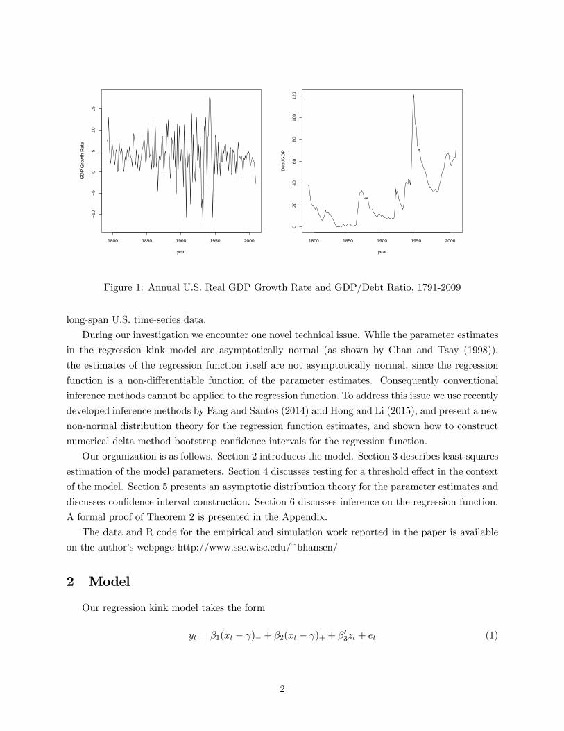
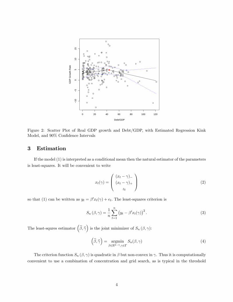
In Figure 2 we display a scatter plot of ( ) along with the fitted regression line and pointwise
90% confidence intervals. (We will discuss estimation in the next section and confidence intervals
in Section 6.) We can see that the fitted regression shows a small positive slope for low debt ratios,
with a kink (threshold) around 44% (displayed as the red square), switching to a negative slope for
debt ratios above that value.
We would like to consider inference in the context of this model, specifically focusing on the
following questions: (1) Is the threshold regression statistically different from a linear regression?
(2) What is the asymptotic distribution of the parameter estimates, and can we construct confidence
intervals for the parameters? (3) Can we construct confidence intervals for the regression line?
3
0 20 40 60 80 100 120
−10
−5
05
1015
Debt/GDP
GD
P G
row
th R
ate
Figure 2: Scatter Plot of Real GDP growth and Debt/GDP, with Estimated Regression Kink
Model, and 90% Confidence Intervals
3 Estimation
If the model (1) is interpreted as a conditional mean then the natural estimator of the parameters
is least-squares. It will be convenient to write
() =
⎛⎜⎝ ( − )−( − )+
⎞⎟⎠ (2)
so that (1) can be written as = 0() + The least-squares criterion is
( ) =1
X=1
¡ − 0()
¢2 (3)
The least-squres estimator³b b´ is the joint minimizer of ( ):³b b´ = argmin
∈R−1∈Γ( ) (4)
The criterion function ( ) is quadratic in but non-convex in . Thus it is computationally
convenient to use a combination of concentration and grid search, as is typical in the threshold
4

literature. Specifically, notice that by concentration we can write
b = argmin∈Γ
min∈R−1
( )
= argmin∈Γ
∗() (5)
where b() are the least-squares coefficients from a regression of on the variables () for fixed
, and
∗() =
³b() ´ = 1
X=1
³ − b()0()´2
is the concentrated sum-of-squared errors function. The solution to (5) can be found numerically
by a grid search over . After b is found then the coefficient estimates b are obtained by standardleast squares of on (b) . We write the fitted regression function as
= b0(b) + b (6)
In (6), b are the (non-linear) least-squares residuals. An estimate of error variance 2 = 2 is
b2 = 1
X=1
b2 = ∗(b)To illustrate, consider the U.S. growth regression for 1792-2009. First, we set the parameter
space Γ for the threshold parameter as Γ = [10 70], so that at least 5% of the sample and 10% of
the support of the threshold variable are below the lower bound and above the upper bound. We
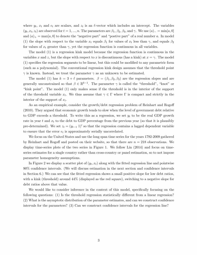
then approximate the minimization (5) by computing ∗() on a discrete grid with increments 01(which has 601 gridpoints). At each gridpoint for we estimated the least-squares coefficients and
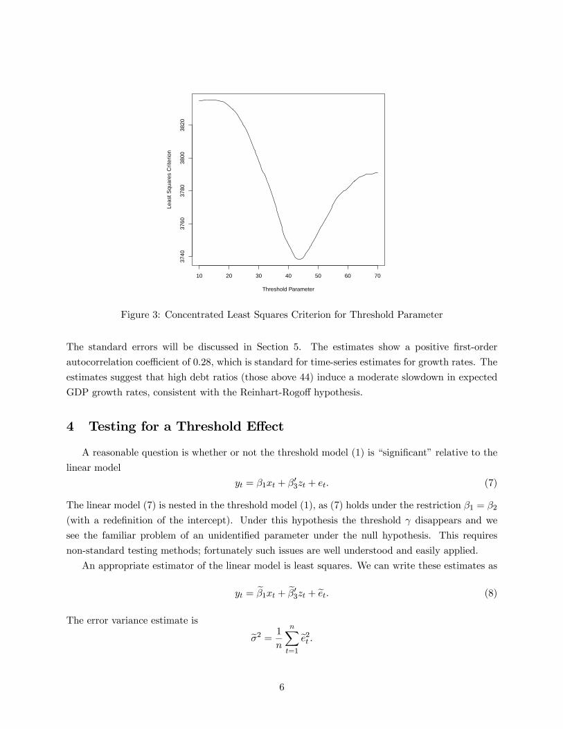
computed the least-squares criterion ∗(). This criterion is plotted as a function of in Figure3. We observe that the function is reasonably smooth and has a well defined global minimum, but
the criterion is not well described as quadratic. The relative smoothness of the plot suggests that
our choice for the grid evaluation is sufficiently fine to obtain the global minimum. The criterion
is minimized at b = 438 Interestingly, this threshold estimate is very close to that found by Lin(2014) for the U.S. using a different data window and quite different empirical framework.
The parameter estimates from this fitted regression kink model are as follows.
= 0033
(0026)
⎛⎜⎝−1 − 438
(121)
⎞⎟⎠−
− 0067
(0048)
⎛⎜⎝−1 − 438
(121)
⎞⎟⎠+
+ 028
(009)
−1 + 378
(069)
+ bb2 = 172
5
10 20 30 40 50 60 70
3740
3760
3780
3800
3820
Threshold Parameter
Leas
t Squ
ares
Crit
erio
n
Figure 3: Concentrated Least Squares Criterion for Threshold Parameter
The standard errors will be discussed in Section 5. The estimates show a positive first-order
autocorrelation coefficient of 028, which is standard for time-series estimates for growth rates. The
estimates suggest that high debt ratios (those above 44) induce a moderate slowdown in expected
GDP growth rates, consistent with the Reinhart-Rogoff hypothesis.
4 Testing for a Threshold Effect
A reasonable question is whether or not the threshold model (1) is “significant” relative to the
linear model
= 1 + 03 + (7)
The linear model (7) is nested in the threshold model (1), as (7) holds under the restriction 1 = 2
(with a redefinition of the intercept). Under this hypothesis the threshold disappears and we
see the familiar problem of an unidentified parameter under the null hypothesis. This requires
non-standard testing methods; fortunately such issues are well understood and easily applied.
An appropriate estimator of the linear model is least squares. We can write these estimates as
= e1 + e03 + e (8)
The error variance estimate is e2 = 1
X=1
e2
6

For example, the estimates of the linear model for our empirical example are as follows.
= − 0008
(0013)
−1 + 030
(009)
−1 + 290
(062)
+ e (9)
e2 = 176The estimates show a postive first-order autocorrelation coefficient, and a near zero coefficient on
the debt ratio.
A standard test for the null hypothesis of the linear model (7) against the threshold model (1)
is to reject 0 : 1 = 2 for large values of the F-type statistic
=¡e2 − b2¢b2
For example, for our empirical example we can compute that = 566.
To describe the distribution theory for the test statistic, we need to be precise about the
stochastic assumptions on the model. We require the following regularity conditions
Assumption 1 For some 1
1. ( ) is strictly stationary, ergodic, and absolutely regular with mixing coefficients () =
(−) for some ( − 1)
2. ||4 ∞, ||4 ∞, and kk4 ∞
3. inf∈Γ det() 0 where () = (()()0)
4. has a density function () satisfying () ≤ ∞
5. ∈ Γ where Γ is compact
Assumption 1.1 & 1.2 are standard weak dependence conditions which are sufficient for a central
limit theorem. The choice of involves a trade-off between the allowable degree of serial dependence
and the number of finite moments. For independent observations we can set arbitrarily close to
one. Assumption 1.3 is an identification condition, requiring that the projection coefficients be well
defined for all values of in the parameter space Γ. Assumption 1.4 requires that the threshold
variable has a bounded density function.
The following is implied by Theorem 3 of Hansen (1996).
Theorem 1 Suppose that Assumption 1 holds and is a martingale difference sequence. Under
0 : 1 = 2
→ sup∈Γ
()0()−1()2 (10)
7

where () is a zero-mean Gaussian process with covariance kernel
((1)(2)) = ¡(1)(2)
02¢ (11)
Theorem 1 shows that the asymptotic null distribution of the threshold F statistic can be writ-
ten as the supremum of a stochastic process. In addition to Assumption 1, Theorem 1 adds the
regularity condition that the error is a martingale difference sequence. This is a sufficient condi-
tion, and convenient, but is not essential. What is important is that the best fitting approximation
in the regression kink model is the linear model so that the central limit theorem applies for all ,
and that the regression scores are uncorrelated so that the covariance kernel takes the simple form
(11) rather than a HAC form.
The limiting distribution (10) is non-standard and cannot be tabulated. However, as shown by
Hansen (1996), it is simple to simulate approximations to (10) using a multiplier bootstrap, and
thus asymptotically valid p-values can be calculated. The following is the recommended algorithm.
Algorithm 1: Testing for a Regression Kink with an Unknown Threshold
1. Generate iid draws from the (0 1) distribution.
2. Set ∗ = e where e are the OLS residuals from the fitted linear regression (8).
3. Using the observations (∗ ), estimate the linear model (8) and the regression kink model(6) and compute the error variance estimates e∗2 and b∗2 and the F-statistic
∗ =¡e∗2 − b∗2¢b∗2
4. Repeat this times, so as to obtain a sample ∗(1) ∗() of simulated F statistics.
5. Compute the p-value as the percentage of simulated F statistics which exceed the actual
value:
=1
X=1
1 ( ∗() ≥ )
6. If desired, compute the level critical value as the empirical 1− quantile of the simulatedF statistics ∗(1) ∗()
7. Reject 0 in favor of 1 at significance level if , or equivalently if
The number of bootstrap replications should be set fairly large to ensure accuracy of the
p-value . For example, if = 10 000 then is approximately within 0006 of its limiting
(large ) value. Fortunately, the computational cost is minimal. For example, my office computer
computed all the empirical calculations reported in this paper in just one minute, including two
separate bootstrap simulations using 10,000 replications each. (The calculations were performed
8
in R. The code implements the multiplier bootstrap efficiently by executing all 10,000 regressions
simultaneously, exploiting the fact that the regressors are common across the boostrap replications.)
Returning to the U.S. GDP example, as we said earlier the empirical value of the F statistic is
= 566. The multiplier bootstrap p-value is 015 and the bootstrap estimate of the 10% critical
value is 7.1. Thus the test does not reject the null hypothesis of linearity in favor of the regression
kink model at the 10% level.
The multiplier bootstrap method does not account for the time-series nature of the observations
and thus can be expected to exhibit some finite sample distortions. To investigate this possibility we
present a simple simulation experiment calibrated on the empirical example. Our data generating
process is
= 1 ( − )− + 2 ( − )+ + 3−1 + 4 +
∼ (0 2)
To evaluate size, we set 1 = 2 = 0 3 = 03, 4 = 3, and 2 = 16 to match the estimates
(9). We fix to equal the empirical values of debt/GDP for the U.S, and set = 218 as in the
empirical example. We generated 10,000 samples from this process. To speed computation, for all
simulations in the paper we evaluate Γ = [10 70] using a grid with increments of 1, which reduces
the number of gridpoints to 61. The number of bootstrap replications for each simulated sample
was set at = 1000.
We first evalualated the size of the threshold test. At the nominal 10% significance level, we
found the simulation size to be 10.6%. Thus, the test exhibits no meaningful size distortion.
Second, we evaluated the power of the test. We used the same parameterization as above, but
now set 1 = 0 and = 40 and vary 2 from 0 to −016 in steps of 002. The power is presented inTable 1. What we can see is that the test has increasing power in 2 and had reasonable ability to
detect changes as small as 008. Examining the point estimates of the threshold model, we see that
the estimate of the difference in regression slopes is b1 − b2 = 010, where the simulation suggeststhe power should be about 70%, which is reasonable but modest. It follows that our empirical
p-value of 15% could be due to the modest power of the test. We conclude that the threshold test
is inconclusive regarding the question of whether or not there is a regression kink effect in GDP
growth due to high debt.
Table 1: Power of Threshold F test with Multiplier Bootstrap, Nominal Size 10%
2
−002 −004 −006 −008 −010 −012 −014 −016Power 014 024 038 054 072 085 093 098
9

5 Inference on the Regression Coefficients
In this section we consider the distribution theory for the least-squares estimates of the regres-
sion kink model with unknown threshold under the assumption that the threshold is identified.
In an ideal context we might consider (1) as the true regression function, so that the error has
conditional mean zero. To allow extra generality, we will not impose this condition. Instead, we
will view (1) as the best approximation in the sense that it minimizes squared error loss. We define
the best approximation as (pseudo)-true values (0 0) which minimize the squared loss
( ) = ¡ − 0()
¢2 (12)
As in our analysis of estimation, we can define the minimizers by concentration. Let () be
the minimizer of ( ) over for fixed , this is () = (()()0)−1 (()). Under
Assumption 1.3, () is uniquely defined for all ∈ Γ. The concentrated squared loss is then
∗ () = (() ) = ¡ − ()0()
¢2
By concentration, 0 is the minimizer of ∗() and 0 = (0)
We will require that the minimizer 0 is unique. This excludes the case of a best-fitting linear
model (in which case ∗() is a constant function) and the case of multiple best-fitting thresholdparameters .
To simplify our proof of consistency, we also impose that the parameter space for is compact,
though this assumption could be relaxed by a more detailed argument.
Assumption 2
1. 0 = argmin∈Γ∗ () is unique.
2. ∈ ⊂ R−1 where is compact.
Chan and Tsay (1998) showed that the least-squares estimates in the continuous threshold
autoregressive model, including both the slope and threshold coefficients, are jointly asymptotically
normal. We extend their distribution theory to the regression kink model with unknown threshold.
Set = ( ), 0 = (0 0),
() = −
() =
Ã()
−11 ( )− 21 ( )
!
and = (0).
Theorem 2 Under Assumption 1
√³b − 0
´→ (0 )
10
where = −1−1, =P∞
=−∞³
0++
´and
= ¡
0
¢+
⎛⎜⎜⎜⎜⎝0 0 0 1 ( 0)
0 0 0 1 ( 0)
0 0 0 0
1 ( 0) 1 ( 0) 0 0
⎞⎟⎟⎟⎟⎠A formal proof of Theorem 2 is presented in the Appendix.
Notice that the slope and threshold estimates are jointly asymptotically normal with√ con-
vergence rate, and the slope and threshold estimates have a non-zero asymptotic covariance. In
contrast, in the conventional non-continuous threshold model the threshold estimate b is rate consistent with a non-standard asymptotic distribution, and the slope coefficient estimates are as-
ymptotically independent of the threshold estimate. The difference in the regression kink model is
because the regression function is continuous. Consequently, the least-squares criterion is continu-
ous in the parameters (though not differentiable) and asymptotically locally quadratic.
The asymptotic distribution does not require the model to be correctly specified, so the error
need not be a martingale difference sequence. Thus (in general) the covariance matrix takes a
HAC form. When the regression is dynamically well specified (by appropriate inclusion of lagged
variables) then the matrix will simplify to = ¡
02
¢. As our application includes a lagged
dependent variable, we use this simplification in practice.
The second term in the definition of is zero when the threshold model is correctly specified
so that (|) = 0. However, in the case of model misspecification (so that the regression is a
best approximation) then the second term can be non-zero.
We suggest the following estimate of the asymptotic covariance matrix (assuming uncorrelat-
edness). Set b =
Ã(b)
−b11 ( b)− b21 ( b)!
and b = b−1 b b−1, b = 1−
P=1
bb 0b2 , and
b = 1
X=1
⎛⎜⎜⎜⎜⎝ bb 0 +
⎛⎜⎜⎜⎜⎝⎡⎢⎢⎢⎢⎣
0 0 0 b1 ( b)0 0 0 b1 ( b)0 0 0 0b1 ( b) b1 ( b) 0 0
⎤⎥⎥⎥⎥⎦⎞⎟⎟⎟⎟⎠⎞⎟⎟⎟⎟⎠
We divide by − rather than for the definition of b as an ad hoc degree-of-freedom adjustment.Given b , standard errors for the coefficient estimates are found by taking the square roots of thediagonal elements of −1b . If the regression is dynamically misspecified (for example, if no laggeddependent variable is included) then b could be formed using a standard HAC estimator.
Asymptotic confidence intervals for the coefficients could then be formed using the conventional
11

rule, e.g. for a 95% interval for 1, b1± 196(b1). Theorem 2 shows that such confidence intervals
have asymptotic correct coverage.
In small samples, however, the asymptotic confidence intervals may have poor coverage. As
shown in Figure 2, the least-squares critierion is non-quadratic with respect to the threshold pa-
rameter , meaning that quadratic (e.g. normal) approximations may be poor unless sample sizes
are quite large. In this context better coverage can be obtained by test-inversion confidence sets.
This is particularly convenient for the threshold parameter , as a test inversion confidence region
is a natural by-product of the computation of the least-squares minimization. Specifically, to test
the hypothesis 0 : = 0 against 1 : 6= 0, the criterion-based test is to reject for large values
of the F-type statistic (0) where
() =¡b2()− b2¢b2 (13)
and b2() = ∗() is the estimator of the error variance when is fixed. Given the asymptotic
normality of Theorem 2, this test has an asymptotic 21 distribution under 0. Thus for a nominal
level test we can take the critical value 1− from the 21 distribution. A nominal 1− asymptoticconfidence interval for can then be formed by test inversion: the set of for which () is smaller
the 21 critical value:
= { : () ≤ 1−}
Given that b2() has already been calculated on a grid (for estimation), we have () on the samegrid as a by-product. The interval is then obtained as the set of gridpoints for which ()
is smaller than 1−.To illustrate, examine Figure 4. Here we have plotted the statistic () from (13) as a function
of . By construction, the statistic is non-negative and hits 0 at = b. We have drawn in theasymptotic 90% critical value 9 = 27 using the blue dashed line. The points of intersection
indicate the ranges for the asymptotic confidence interval, and shown on the graph by the blue
dashed arrows to the horizontal axes.
Further improvements in coverage accuracy can be obtained via a bootstrap. We recommend a
simple wild bootstrap. Here are the steps.
Algorithm 2: Wild Bootstrap Confidence Intervals for Parameters
1. Generate iid draws from the (0 1) distribution.
2. Set ∗ = b where b are the LS residuals from the fitted regression kink model (6).
3. Set ∗ = b0(b) + ∗ , where ( ) are the sample observations, and (b b) are the least-squares estimates.
4. Using the observations (∗ ), estimate the the regression kink model (6), parameterestimates (b∗ b∗), and b∗2 = −1
P=1 b∗2 , where b∗ = ∗ − b∗0(b∗)
12

10 20 30 40 50 60 70
01
23
45
Threshold Parameter
Thr
esho
ld F
Sta
tistic
Bootstrap Critical ValueAsymptotic Critical Value
Figure 4: Confidence Interval Construction for Threshold
5. Calculate the F-statistic for
∗ =¡b∗2(b)− b∗2¢b∗2
where b∗2(b) = −1P
=1 b∗ (b)2 and b∗ (b) = ∗ − b∗(b)0(b)6. Repeat this times, so as to obtain a sample of simulated coefficient estimates (b∗ b∗) andF statistics ∗
7. Create 1− bootstrap confidence intervals for the coefficients 1 2 and 3 by the symmetricpercentile method: the coefficient estimates plus and minus the (1−) quantile of the absolutecentered bootstrap estimates. E.g., for 1 the interval is b1±∗1 where ∗1 is the (1−) quantileof |b∗1 − b1|.
8. Calculate the 1− quantile ∗1− of the simulated F statistics ∗
9. Create a 1 − bootstrap confidence interval for as the set of for which the empirical F
statistics () (13) are smaller than the bootstrap critical value ∗1−
∗ =© : () ≤ ∗1−
ª
This wild bootstrap algorithm can be computed concurrently with the multiplier bootstrap used
for the threshold test, resulting in efficient computation.
Again for illustration the confidence interval construction can be seen via Figure 4, where
the statistic () is plotted against . The bootstrap 90% critical value 3.3 (calculated with
13
= 10 000 bootstrap replications) is plotted as the red dotted line. The points of intersection
indicate the ranges of the confidence interval, and are indicated on the figure by the red dotted
arrows to the horizontal axis. Since the bootstrap critical value is larger than the asymptotic critical
value, the asymptotic interval is a subset of the bootstrap confidence interval.
Before presenting the empirical results we report results from our simulation experiment to
assess the performance of the methods. The data generating process is identical to that used in the
previous section. As before, 2 is the key free parameter, controlling the strength of the threshold
effect, and the remaining parameters and variables are set to match the empirical data. As before,
we generated 10 000 simulated samples and used = 1000 bootstrap replications for each sample.
In Tables 2 and 3 we report the coverage rates of nominal 90% intervals for the parameters 2 and
.
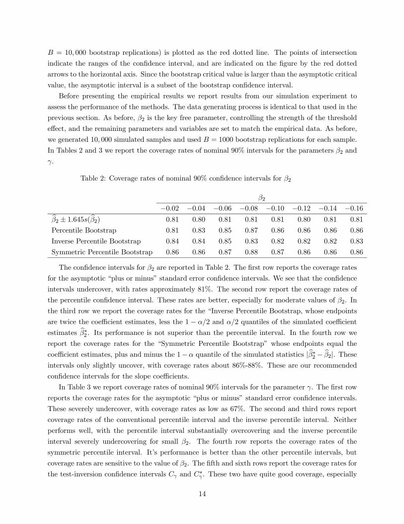
Table 2: Coverage rates of nominal 90% confidence intervals for 2
2
−002 −004 −006 −008 −010 −012 −014 −016b2 ± 1645(b2) 081 080 081 081 081 080 081 081
Percentile Bootstrap 081 083 085 087 086 086 086 086
Inverse Percentile Bootstrap 084 084 085 083 082 082 082 083
Symmetric Percentile Bootstrap 086 086 087 088 087 086 086 086
The confidence intervals for 2 are reported in Table 2. The first row reports the coverage rates
for the asymptotic “plus or minus” standard error confidence intervals. We see that the confidence
intervals undercover, with rates approximately 81%. The second row report the coverage rates of
the percentile confidence interval. These rates are better, especially for moderate values of 2. In
the third row we report the coverage rates for the “Inverse Percentile Bootstrap, whose endpoints
are twice the coefficient estimates, less the 1 − 2 and 2 quantiles of the simulated coefficient
estimates b∗2 . Its performance is not superior than the percentile interval. In the fourth row wereport the coverage rates for the “Symmetric Percentile Bootstrap” whose endpoints equal the
coefficient estimates, plus and minus the 1− quantile of the simulated statistics |b∗2 − b2|. Theseintervals only slightly uncover, with coverage rates about 86%-88%. These are our recommended
confidence intervals for the slope coefficients.
In Table 3 we report coverage rates of nominal 90% intervals for the parameter . The first row
reports the coverage rates for the asymptotic “plus or minus” standard error confidence intervals.
These severely undercover, with coverage rates as low as 67%. The second and third rows report
coverage rates of the conventional percentile interval and the inverse percentile interval. Neither
performs well, with the percentile interval substantially overcovering and the inverse percentile
interval severely undercovering for small 2. The fourth row reports the coverage rates of the
symmetric percentile interval. It’s performance is better than the other percentile intervals, but
coverage rates are sensitive to the value of 2. The fifth and sixth rows report the coverage rates for
the test-inversion confidence intervals and ∗ . These two have quite good coverage, especially
14
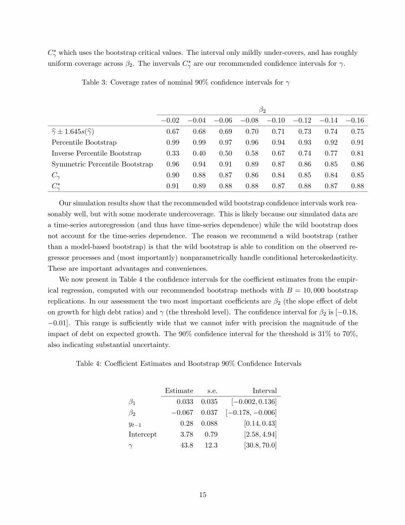
∗ which uses the bootstrap critical values. The interval only mildly under-covers, and has roughlyuniform coverage across 2. The invervals
∗ are our recommended confidence intervals for .
Table 3: Coverage rates of nominal 90% confidence intervals for
2
−002 −004 −006 −008 −010 −012 −014 −016b ± 1645(b) 067 068 069 070 071 073 074 075
Percentile Bootstrap 099 099 097 096 094 093 092 091
Inverse Percentile Bootstrap 033 040 050 058 067 074 077 081
Symmetric Percentile Bootstrap 096 094 091 089 087 086 085 086
090 088 087 086 084 085 084 085
∗ 091 089 088 088 087 088 087 088
Our simulation results show that the recommended wild bootstrap confidence intervals work rea-
sonably well, but with some moderate undercoverage. This is likely because our simulated data are
a time-series autoregression (and thus have time-series dependence) while the wild bootstrap does
not account for the time-series dependence. The reason we recommend a wild bootstrap (rather
than a model-based bootstrap) is that the wild bootstrap is able to condition on the observed re-
gressor processes and (most importantly) nonparametrically handle conditional heteroskedasticity.
These are important advantages and conveniences.
We now present in Table 4 the confidence intervals for the coefficient estimates from the empir-
ical regression, computed with our recommended bootstrap methods with = 10 000 bootstrap
replications. In our assessment the two most important coefficients are 2 (the slope effect of debt
on growth for high debt ratios) and (the threshold level). The confidence interval for 2 is [−018−001]. This range is sufficiently wide that we cannot infer with precision the magnitude of theimpact of debt on expected growth. The 90% confidence interval for the threshold is 31% to 70%,
also indicating substantial uncertainty.
Table 4: Coefficient Estimates and Bootstrap 90% Confidence Intervals
Estimate s.e. Interval
1 0033 0035 [−0002 0136]2 −0067 0037 [−0178−0006]−1 028 0088 [014 043]
Intercept 378 079 [258 494]
438 123 [308 700]
15
6 Inference on the Regression Kink Function
In this section we consider inference on the regression kink function
() = 0() (14)
where
() =
⎛⎜⎝ (− )−(− )+
⎞⎟⎠
Our theory will treat ( ) as fixed, even though we will display the estimates as a function of .
(Thus we focus on pointwise confidence intervals for the regression function.)
The plug-in estimate of () is (b) = b0(b) In our empirical example, we display in Figure 2(b) as a function of , with fixed at the sample mean of .
Since Theorem 2 shows that b is asymptotically normal, it might be conjectured that (b) willbe as well. This conjecture turns out to be incorrect. While () is a continuous function of , it
is not differentiable at = . As discussed in a recent series of papers (Hirano and Porter (2012),
Woutersen and Ham (2013), Fang and Santos (2014), Fang (2014) and Hong and Li (2015), the
non-differentiability means that (b) will not be asymptotically normal at 0 = , and asymptotic
normality is likely to be a poor approximation for 0 close to .
While the regression kink function () is not differentiable at = , it is directionally dif-
ferentiable at all points, meaning that both left and right derivatives are defined. The directional
derivative of a function () : R → R in the direction ∈ R is
() = lim↓0
( + )− ()
(15)
(See Shapiro (1990).) The primary difference with the conventional notion of a derivative is that
() is allowed to depend on the direction in which the derivative is taken. For continuously
differentiable functions the directional derivative is linear in . For example, if () = 0 is linear,then () = 0. If () is continuously differentiable in then () =
¡()
¢0. However, if
() is continuous but not continuously differentiable the directional derivative will be non-linear
in .
In the case of (14), we can calculate that the directional derivative of () in the direction
= ( ) is
() = ()0 + () (16)
where
() =
⎧⎪⎨⎪⎩−1 if
−11 ( 0)− 21 ( ≥ 0) if =
−2 if
(17)
16
The directional derivative () is linear for 6= but non-linear for = , with a slope to the
left of −1 and a slope to the right of −2.Conventional asymptotic theory for functions of the form (b) requires that the function ()
be continuously differentiable. Shapiro (1991, Theorem 2.1) and Fang and Santos (2014, Corollary
2.1) have generalized this to the case of directional differentiability. They have established that
if√³b − 0
´→ Z ∼ (0 ) and () is continuous in then
√³(b)− (0)
´→ (Z).
In the classic case where () is continuously differentiable, the limiting distribution specializes to
(Z) =¡()
¢0Z ∼
³0¡()
¢0¡()
¢´, so their result is a strict generalization of the
Delta Method.
Since (16)-(17) is continuous in , we can immediately deduce the asymptotic distribution of
the regression estimate.
Theorem 3√³(b)− (0)
´→ (Z) where Z ∼ (0 ) and () is defined in (16)-(17).
For 6= 0 the asymptotic distribution in Theorem 3 is normal, but for = 0 it is a non-linear
transformation of a normal random vector. At = 0 the asymptotic distribution will be biased,
with the direction of bias depending on the relative magnitudes of 1 and 2. For example, if 1 = 1
and 2 = −1 then () = | | so the asymptotic distribution in Theorem 3 will have a positive
mean while if the signs of the coefficients are reversed then () = − | | and the asymptoticdistribution in Theorem 3 will have a negative mean.
This non-normality implies that classical confidence intervals will have incorrect asymptotic
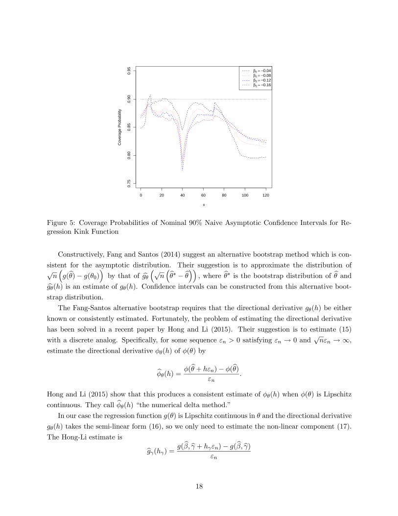
coverage. We illustrate this in Figure 5 by a continuation of our simulation experiment. Using the
same simulation design as in the previous section, and varying 2 from −004 to −016 in steps of004, we plot the coverage probability of classical (naive) nominal 90% pointwise confidence inter-
vals, plotting the coverage as a function of . The asymptotic theory predicts that the confidence
intervals will have asymptotically correct 90% coverage for 6= 0 but not for = 0, so we should
expect coverage to be better for distinct from = 40 , but deteriorating for near = 40. Indeed,
we see that the coverage rates vary from near 90% for small to approximately 77% at = 40.
The distortion from the nominal coverage is sensitive to 2, with the distortion steepening as 2
increases. We can also see that the coverage rates are less than the nominal 90% for large values
of , which is not predicted from the asymptotic theory, and these distortions are more severe for
small values of 2. This appears to be a small-sample issue (a finite sample bias in the regression
estimate; there are only seven observations where ≥ 80) and thus unrelated to the asymptoticnon-normality of Theorem 3.
We might hope that bootstrap methods would improve the coverage probabilities, but this is a
false hope. As shown by Fang and Santos (2014, Corollary 3.1), the non-normality of Theorem 3
implies that the conventional bootstrap will be inconsistent. Indeed, we investigated the coverage
probabilities of confidence intervals constructed using the percentile and inverse percentile methods,
and their coverage rates are similar to that shown in Figure 5 (though less distortion for large ),
so are not displayed here.
17
0 20 40 60 80 100 120
0.75
0.80
0.85
0.90
0.95
x
Cov
erag
e P
roba
bilit
y
β2 = −0.04β2 = −0.08β2 = −0.12β2 = −0.16
Figure 5: Coverage Probabilities of Nominal 90% Naive Asymptotic Confidence Intervals for Re-
gression Kink Function
Constructively, Fang and Santos (2014) suggest an alternative bootstrap method which is con-
sistent for the asymptotic distribution. Their suggestion is to approximate the distribution of√³(b)− (0)
´by that of b ³√³b∗ − b´´ where b∗ is the bootstrap distribution of b andb() is an estimate of (). Confidence intervals can be constructed from this alternative boot-
strap distribution.
The Fang-Santos alternative bootstrap requires that the directional derivative () be either
known or consistently estimated. Fortunately, the problem of estimating the directional derivative
has been solved in a recent paper by Hong and Li (2015). Their suggestion is to estimate (15)
with a discrete analog. Specifically, for some sequence 0 satisfying → 0 and√ → ∞,
estimate the directional derivative () of () by
b() = (b + )− (b)
Hong and Li (2015) show that this produces a consistent estimate of () when () is Lipschitz
continuous. They call b() “the numerical delta method.”In our case the regression function () is Lipschitz continuous in and the directional derivative
() takes the semi-linear form (16), so we only need to estimate the non-linear component (17).
The Hong-Li estimate is
b() = (b b + )− (b b)
18
where we have written (b b) = (b). Thus our estimate of the full directional derivative isb() = (b)0 + (b b + )− (b b)
Evaluated at = ( ) =³√
³b∗ − b´ √ (b∗ − b)´, the bootstrap estimate of the distribu-
tion of (b)− (0) is
∗ = (b)0 ³b∗ − b´+ (b b +√ (b∗ − b))− (b b)√
Hong and Li (2015) show that if the function () is a convex function of then upper one-
sided confidence intervals for constructed using ∗ uniformly control size, but lower one-sidedconfidence intervals will not, and the converse holds when () is a concave function. In our case,
the function () is a convex function of if 1 ≤ 2 but is concave if 1 ≥ 2. Thus neither one-
sided confidence intervals will uniformly control size. Their suggestion is to instead use two-sided
symmetric confidence intervals, as these will be asymptotically conservative.
Let ∗1− denote the (1−) quantile of the variable |∗|. The symmetric bootstrap confidenceinterval for (0) is (b)± ∗1−. We call this the numerical delta method bootstrap interval.
An important issue is setting , the increment for the numerical derivative. While the general
theory of Hong and Li (2015) requires√ →∞ , in the context of this model they recommend
= −12, though they provide no guidance for selection of We follow their advice and set
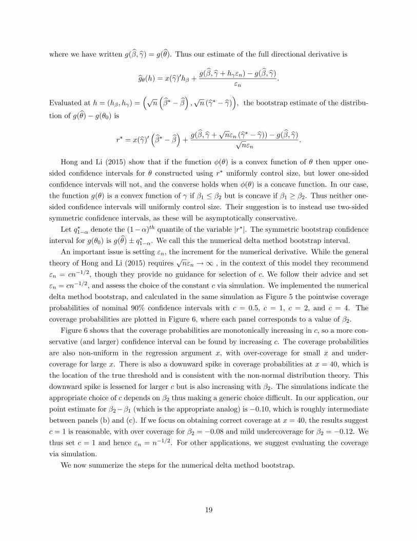
= −12, and assess the choice of the constant via simulation. We implemented the numericaldelta method bootstrap, and calculated in the same simulation as Figure 5 the pointwise coverage
probabilities of nominal 90% confidence intervals with = 05, = 1, = 2, and = 4. The
coverage probabilities are plotted in Figure 6, where each panel corresponds to a value of 2.
Figure 6 shows that the coverage probabilities are monotonically increasing in , so a more con-
servative (and larger) confidence interval can be found by increasing . The coverage probabilities
are also non-uniform in the regression argument , with over-coverage for small and under-
coverage for large . There is also a downward spike in coverage probabilities at = 40, which is
the location of the true threshold and is consistent with the non-normal distribution theory. This
downward spike is lessened for larger but is also increasing with 2. The simulations indicate the
appropriate choice of depends on 2 thus making a generic choice difficult. In our application, our
point estimate for 2−1 (which is the appropriate analog) is −010, which is roughly intermediatebetween panels (b) and (c). If we focus on obtaining correct coverage at = 40, the results suggest
= 1 is reasonable, with over coverage for 2 = −008 and mild undercoverage for 2 = −012. Wethus set = 1 and hence = −12. For other applications, we suggest evaluating the coveragevia simulation.
We now summerize the steps for the numerical delta method bootstrap.
19
0 20 40 60 80 100 120
0.80
0.85
0.90
0.95
1.00
x
Cov
erag
e P
roba
bilit
y
εn = 0.5n−0.5
εn = 1n−0.5
εn = 2n−0.5
εn = 4n−0.5
(a) 2 = −004
0 20 40 60 80 100 120
0.80
0.85
0.90
0.95
1.00
x
Cov
erag
e P
roba
bilit
y
εn = 0.5n−0.5
εn = 1n−0.5
εn = 2n−0.5
εn = 4n−0.5
(b) 2 = −008
0 20 40 60 80 100 120
0.80
0.85
0.90
0.95
1.00
x
Cov
erag
e P
roba
bilit
y
εn = 0.5n−0.5
εn = 1n−0.5
εn = 2n−0.5
εn = 4n−0.5
(c) 2 = −012
0 20 40 60 80 100 120
0.80
0.85
0.90
0.95
1.00
x
Cov
erag
e P
roba
bilit
y
εn = 0.5n−0.5
εn = 1n−0.5
εn = 2n−0.5
εn = 4n−0.5
(d) 2 = −016
Figure 6: Coverage Probabilities of Nominal 90% Numerical Delta Method Bootstrap Intervals
20

Algorithm 3: Numerical Delta Method Bootstrap Confidence Intervals for Regres-
sion Kink Function at a fixed value of ( )
1. Follow steps 1-3 of the wild bootstrap of Algorithm 2
2. Set (b) = ((− b)− (− b)+ 0)03. Set = −12
4. Set ∗ = (b)0 ³b∗ − b´+ ³(b b +√ (b∗ − b))− (b b)´ √5. Repeat times, so as to obtain a sample of simulated estimates ∗
6. Calculate ∗1−, the (1− ) quantile of the simulated |∗|
7. Set the 1− confidence interval for (0) as [(b)− ∗1− (b) + ∗1−]
This is numerically quite simple to implement, although step 4 is unusual for a bootstrap
procedure. For confidence interval bands, steps 2 through 7 need to be repeated for each value of
( ) considered.
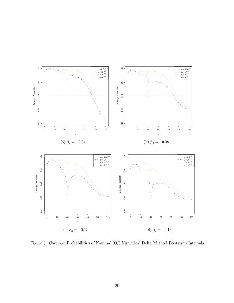
We implemented the numerical delta method bootstrap using the rule = −12 on the U.S.growth regression for = 05, = 1, = 2, and = 4, and plotted the pointwise 90% confidence
intervals in Figure 7. Numerically, this means that Algorithm 3 was applied with set at the
sample mean of and evaluated on a grid from 1 to 120. The confidence intervals widen as
increases, except at = b.Following the recommendation of our simulation study we take the second estimator (with
= −12) as our preferred choice, and this is plotted in Figure 2 with the dashed blue lines.The confidence intervals are sufficiently wide that it is unclear if the true regression function is flat
or downward sloping. The confidence intervals reveal that by using the U.S. longspan data alone,
the estimates of the regression kink model are not sufficiently precise to make a strong conclusion
about whether or not there is a negative effect of debt levels on GDP growth rates.
7 Conclusion
This paper developed a theory of estimation and inference for the regression kink model with
an unknown threshold and applied it to study the growth & debt threshold problem of Reinhart
and Rogoff (2010). An interesting theoretical contribution is the finding that the estimate of
the regression function is non-normal due to non-differentiability, and confidence intervals can be
formed using the recent inference methods of Fang and Santos (2014) and Hong and Li (2015).
We apply the method to the long-span time-series U.S. data developed by Reinhart and Ro-
goff (2010). Our point estimates are consistent with the Reinhart-Rogoff hypothesis of a growth
slowdown when debt levels exceed a threshold. However, the formal evidence for the presence of
21
0 20 40 60 80 100 120
Debt/GDP
GD
P G
row
th R
ate
−8
−4
04
8
εn = 0.5n−0.5
εn = 1n−0.5
εn = 2n−0.5
εn = 4n−0.5
Figure 7: Estimated Regression Kink Function and 90% Numerical Delta Method Confidence
Intervals
the threshold effect is inconclusive, and our confidence intervals for the regression function are
sufficiently wide that the effect of debt on growth is difficult to detect.
An important cavaet is that our empirical results are based only on a single time-series (the
United States), thus ignoring the information in other nations’ experiences. This has the advantage
of not imposing homogeneity, but also may reduce precision and power. It would be useful to extend
the results here to panel data analysis.
8 Appendix
Proof of Theorem 2:
By the definition (4), b minimizes () defined in (3), which we can write as () =1
P=1 ()
2 with () = − 0() Thus b approximately solves the first-order condition1
P=1(b) = 0 where () = ()(). The pseudo-true value 0 minimizes () = ( )
and thus solves (0) where () =12() = (). Define () = −
0().
Andrews (1994), Section 3.2, shows that Theorem 2 will hold under the following conditions.
Condition 1 b → 0
Condition 2 1√
P=1 → (0 )
Condition 3 () is continuous in and (0) =
22

Condition 4 () =1√
P=1 (()−()) is stochastically equicontinuous
We first establish Condition 1. Since () is continuous in , () and ()2 are continuous in
. Recalling definition (2) we have the simple bound k()k2 = 0+ (− )2 ≤ kk2+ 2 + 2
Then by the and Cauchy-Schwarz inequalities,
()2 ≤ 22 + 2
¯̄0()
¯̄2 ≤ 22 + 22 ³kk2 + 2 + 2´
(18)
where = sup {kk : ∈ } and = sup {|| : ∈ Γ} which are finite under Assumption 2.2. Thebound in (18) has finite expectation under Assumption 1.2. Then by Lemma 2.4 of Newey and
McFadden (1994) (which is based on Lemma 1 of Tauchen (1985)), () = ()2 is continuous
and sup∈×Γ | ()− ()| → 0 as → ∞. Lemma 2.4 of Newey and McFadden is stated fori.i.d. observations, but the result only requires application of a weak law of large numbers, which
holds under Assumption 1 by the Ergodic theorem.
Given the compactness of × Γ and the uniqueness of the minimum 0 (by Assumptions 1.2
and 1.1, respectively), Theorem 2.1 of Newey and McFadden (1994) establishes that b → 0 as
→∞ which is Condition 1.
Condition 2 follows by the Herrndorf’s (1984) central limit theorem for strong mixing processes
which holds under Assumption 1.1-1.2.
The following bound will be useful to establish Conditions 3 and 4. Let be any pairwise
product of the variables ( ), and set = 2(2 − 1). Note that Assumption 1.2 implies³ ||2
´12≤ for some ∞. Let () denote the distribution function of , which satisfies
(2)− (1) ≤ |2 − 1| under Assumption 1.4. By Holder’s inequality, we find
|1 (1 ≤ ≤ 2)| ≤³ ||2
´12( |1 (1 ≤ ≤ 2)|)1
≤ ( (2)− (1))1
≤ 1 |2 − 1|1 (19)
One implication of this bound is that (1 ( ≤ )) is uniformly continuous in .
We now establish Condition 3. Note that
() = −
0 (()())
= ¡()()
0¢+
⎛⎜⎜⎜⎜⎝0 0 0 ()1 ( ≤ )
0 0 0 ()1 ( )
0 0 0 0
()1 ( ≤ ) ()1 ( ) 0 0
⎞⎟⎟⎟⎟⎠The elements of this matrix are quadratic functions of , and functions of through moments of
the form (1 ( ≤ )) where is a product of the variables ( ). Since (19) holds we see
that () is continuous in . Evaluated at 0 we find (0) = . Thus Condition 3 holds.
23

We now establish Condition 4 by appealing to Theorem 1, Application 4, case (2.15) of Doukan,
Massart, and Rio (1995). Notice that ∗ () = () −() is a function of as a quadratic, so
the only issue is establishing stochastic equicontinuity with respect to so we simplify notation by
writing the variable as∗ (). Notice as well that the elements of() are of the form 1 ( ≤ )
where is a product of the variables ( ). Under Assumption 1.2, ∗ () has a bounded 2
moment and thus satisfies the needed envelope condition. Furthermore, since the elements are of
the form 1 ( ≤ ), for any 1 and 2, by (19),
k∗ (1)−∗ (2)k2 ≤ 2³kk2 1 (1 ≤ ≤ 2)
´≤
1 |2 − 1|1 (20)
For any 0 set () = −12 and set , = 1 to be an equally spaced grid on Γ. Then
for each ∈ Γ there is a ∈ {1 } such that by (20)³ k∗ ()−()k2
´12≤ 12
12 | − |12 ≤ ¡−2¢ = ()
and thus () = −12 are the 2 bracking numbers and 2() = ln() = |log | is the metricentropy with bracketing. Then equation (2.15) of Doukan, Massart, and Rio (1995) holds under
Assumption 1.1, which is sufficient for their Theorem 1, establishing stochastic equicontinuity of
() and hence Condition 4.
We have established that Conditions 1-4 hold under Assumptions 1 and 2. As discussed above,
this is sufficient to establish Theorem 2. ¥
References
[1] Andrews, Donald W.K. (1994): “Empirical process methods in econometrics,”Handbook of
Econometrics, Vol IV, R.F. Engle and D.L McFadden, eds., 2247-2294. New York: Elsevier.
[2] Caner, Mehmet, Thomas Grennes, and Fritzi Koehler-Geib (2010): “Finding the tipping point-
when sovereign debt turns bad,” Policy Research Working Paper Series 5391, The World Bank.
[3] Caner, Mehmet and Bruce E. Hansen (2004): “Instrumental Variable Estimation of a Thresh-
old Model,” Econometric Theory, 20, 813-843
[4] Card, David, David Lee, Zhuan Pei, Andrea Weber (2012): “Nonlinear policy rules and the
identification and estimation of causal effects in a generalized regression kind design,” NBER
Working Paper 18564.
[5] Card, David, Alexandre Mas and Jesse Rothstein (2008): “Tipping and the dynamics of
segregation,” Quarterly Journal of Economics, 123, 177-218.
[6] Cecchetti, Stephen G, M. S. Mohanty, and Fabrizio Zampolli (2011). “The real effects of debt,”
Economic Symposium Conference Proceedings: Federal Reserve Bank of Kansas City, 145-196.
24

[7] Chan, Kung-Sik (1990): “Testing for threshold autoregression,” The Annals of Statistics 18,
1886-1894.
[8] Chan, Kung-Sik (1991): “Percentage points of likelihood ratio tests for threshold autoregres-
sion,” Journal of the Royal Statistical Society, Series , 53, 691-696.
[9] Chan, Kung-Sik (1993): “Consistency and limiting distribution of the least squares estimator
of a threshold autoregressive model,” The Annals of Statistics, 21, 520-533.
[10] Chan, Kung-Sik and Howell Tong (1990): “On likelihood ratio tests for threshold autoregres-
sion,” Journal of the Royal Statistical Society B, 52, 469-476.
[11] Chan, Kung-Sik and Ruey S. Tsay (1998): “Limiting properties of the least squares estimator
of a continuous threshold autoregressive model,” Biometrika, 45, 413-426.
[12] Cox, Donald, Bruce E. Hansen and Emmanuel Jimenez (2004): “How responsive are private
transfers to income?” Journal of the Public Economics, 88, 2193-2219.
[13] Doukhan, P., P. Massart and E. Rio (1995): “Invariance principles for absolutely regular
empirical processes,” Annales de l’Institut H. Poincare, Probabiltes et Statistiques, 31, 393-
427.
[14] Fang, Zheng (2014) “Optimal plug-in estimators of directionally differentiable functionals,”
working paper, UCSD.
[15] Fang, Zheng and Andres Santos (2014): “Inference on directionally differentiable functions,”
working paper, UCSD.
[16] Ganong, Peter and Simon Jager (2014): “A permutation test and estimation alternatives for
the regression kink design,” working paper, Harvard University.
[17] Hansen, Bruce E. (1996): “Inference when a nuisance parameter is not identified under the
null hypothesis,” Econometrica, 64, 413-430.
[18] Hansen, Bruce E. (1999): “Threshold effects in non-dynamic panels: Estimation, testing and
inference,” Journal of Econometrics, 93, 345-368
[19] Hansen, Bruce E. (2000): “Sample splitting and threshold estimation,” Econometrica, 68,
575-603.
[20] Herrndorf, N. (1984): “A functional central limit theorem for weakly dependent sequences of
random variables,” The Annals of Probability, 12, 141-153.
[21] Hirano, Keisuke and Jack Porter (2012): “Impossibility results for nondifferentiable function-
als,” Econometrica, 80, 1769-1790.
25
[22] Hong, Han and Jessie Li (2015): “The numerical directional delta method,” working paper,
Stanford University.
[23] Landais, Camille (2012): “Assessing the welfare effects of unemployment benefits using the
regression kink design,” working paper, London School of Economics.
[24] Lin, Tzu-Chi (2014): “High-dimensional threshold quantile regression with an application to
debt overhang and economic growth,” working paper, University of Wisconsin.
[25] Newey, Whitney K. and Daniel McFadden (1994): “Large sample estimation and hypothesis
testing,” Handbook of Econometrics, Vol IV, R.F. Engle and D.L McFadden, eds., 2113-2245.
New York: Elsevier.
[26] Porter, Jack and Ping Yu (2014): “Regression discontinuity designs with unknown discontinu-
ity points: Testing and estimation,” working paper, University of Wisconsin.
[27] Ramirez-Rondan, Nelson (2013): “Maximum likelihood estimation of a dy-
namic panel threshold model,” working paper, Central Bank of Peru,
https://sites.google.com/site/teltoramirezrondan/.
[28] Reinhart, Carmen M. and Kenneth S. Rogoff (2010): “Growth in a time of debt,” American
Economic Review: Papers and Proceedings, 100, 573-578.
[29] Seo, Myung Hwan and Oliver Linton (2007): “A smoothed least squares estimator for threshold
regression models,” Journal of Econometrics, 141 704-735.
[30] Shapiro, Alexander (1990): “On concepts of directional differentiability,” Journal of Optimiza-
tion Theory and Applications, 66, 477-487.
[31] Shapiro, Alexander (1991): “Asymptotic analysis of stochastic programs,” Annals of Opera-
tions Research, 30, 169-186.
[32] Tauchen, George (1985): “Diagnostic Testing and Evaluation of Maximum Likelihood Models,”
Journal of Econometrics, 30, 415-443.
[33] Tong, Howell (1983): Threshold Models in Non-linear Time Series Analysis. Lecture Notes in
Statistics, 21, Berlin: Springer.
[34] Tong, Howell (1990): Non-Linear Time Series: A Dynamical System Approach, Oxford Uni-
versity Press, Oxford.
[35] Woutersen, Tiemen and John C. Ham (2013): “Calculating confidence intervals for continuous
and discontinuous functions of parameters,” working paper, University of Arizona.
26