inference on causal effects in a generalized regression ... · inference on causal effects in a...
TRANSCRIPT

DI
SC
US
SI
ON
P
AP
ER
S
ER
IE
S
Forschungsinstitut zur Zukunft der ArbeitInstitute for the Study of Labor
Inference on Causal Effects in aGeneralized Regression Kink Design
IZA DP No. 8757
January 2015
David CardDavid S. LeeZhuan PeiAndrea Weber

Inference on Causal Effects in a Generalized Regression Kink Design
David Card UC Berkeley, NBER and IZA
David S. Lee
Princeton University and NBER
Zhuan Pei Brandeis University
Andrea Weber
University of Mannheim and IZA
Discussion Paper No. 8757 January 2015
IZA
P.O. Box 7240 53072 Bonn
Germany
Phone: +49-228-3894-0 Fax: +49-228-3894-180
E-mail: [email protected]
Any opinions expressed here are those of the author(s) and not those of IZA. Research published in this series may include views on policy, but the institute itself takes no institutional policy positions. The IZA research network is committed to the IZA Guiding Principles of Research Integrity. The Institute for the Study of Labor (IZA) in Bonn is a local and virtual international research center and a place of communication between science, politics and business. IZA is an independent nonprofit organization supported by Deutsche Post Foundation. The center is associated with the University of Bonn and offers a stimulating research environment through its international network, workshops and conferences, data service, project support, research visits and doctoral program. IZA engages in (i) original and internationally competitive research in all fields of labor economics, (ii) development of policy concepts, and (iii) dissemination of research results and concepts to the interested public. IZA Discussion Papers often represent preliminary work and are circulated to encourage discussion. Citation of such a paper should account for its provisional character. A revised version may be available directly from the author.

IZA Discussion Paper No. 8757 January 2015
ABSTRACT
Inference on Causal Effects in a Generalized Regression Kink Design*
We consider nonparametric identification and estimation in a nonseparable model where a continuous regressor of interest is a known, deterministic, but kinked function of an observed assignment variable. This design arises in many institutional settings where a policy variable (such as weekly unemployment benefits) is determined by an observed but potentially endogenous assignment variable (like previous earnings). We provide new results on identification and estimation for these settings, and apply our results to obtain estimates of the elasticity of joblessness with respect to UI benefit rates. We characterize a broad class of models in which a sharp “Regression Kink Design” (RKD, or RK Design) identifies a readily interpretable treatment-on-the-treated parameter (Florens et al. (2008)). We also introduce a “fuzzy regression kink design” generalization that allows for omitted variables in the assignment rule, noncompliance, and certain types of measurement errors in the observed values of the assignment variable and the policy variable. Our identifying assumptions give rise to testable restrictions on the distributions of the assignment variable and predetermined covariates around the kink point, similar to the restrictions delivered by Lee (2008) for the regression discontinuity design. We then use a fuzzy RKD approach to study the effect of unemployment insurance benefits on the duration of joblessness in Austria, where the benefit schedule has kinks at the minimum and maximum benefit level. Our preferred estimates suggest that changes in UI benefit generosity exert a relatively large effect on the duration of joblessness of both low-wage and high-wage UI recipients in Austria. JEL Classification: C13, C14, C31 Keywords: regression discontinuity design, regression kink design, treatment effects,
nonseparable models, nonparametric estimation Corresponding author: Andrea Weber University of Mannheim L7, 3-5, Room 420 68131 Mannheim Germany E-mail: [email protected]
* We thank Diane Alexander, Mingyu Chen, Kwabena Donkor, Martina Fink, Samsun Knight, Andrew Langan, Carl Lieberman, Michelle Liu, Steve Mello, Rosa Weber and Pauline Leung for excellent research assistance. We have benefited from the comments and suggestions of Sebastian Calonico, Matias Cattaneo, Andrew Chesher, Nathan Grawe, Bo Honoré, Guido Imbens, Pat Kline and seminar participants at Brandeis, BYU, Brookings, Cornell, Georgetown, GWU, IZA, LSE, Michigan, NAESM, NBER, Princeton, Rutgers, SOLE, Upjohn, UC Berkeley, UCL, Uppsala, Western Michigan, Wharton and Zürich. Andrea Weber gratefully acknowledges research funding from the Austrian Science Fund (NRN Labor Economics and the Welfare State).

1 Introduction
A growing body of research considers the identification and estimation of nonseparable models with con-
tinuous endogenous regressors in semiparametric (e.g., Lewbel (1998); Lewbel (2000)) and non-parametric
settings (e.g., Blundell and Powell (2003); Chesher (2003); Florens et al. (2008); Imbens and Newey (2009)).
The methods proposed in the literature so far rely on instrumental variables that are independent of the un-
observable terms in the model. Unfortunately, independent instruments are often hard to find, particularly
when the regressor of interest is a deterministic function of an endogenous assignment variable. Unemploy-
ment benefits, for example, are set as function of previous earnings in most countries. Any variable that is
correlated with benefits is likely to be correlated with the unobserved determinants of previous wages and is
therefore unlikely to satisfy the necessary independence assumptions for a valid instrument.
Nevertheless, many tax and benefit formulas are piece-wise linear functions with kinks in the relation-
ship between the assignment variable and the policy variable caused by minimums, maximums, and discrete
shifts in the marginal tax or benefit rate. As noted by Classen (1977a), Welch (1977), Guryan (2001),
Dahlberg et al. (2008), Nielsen et al. (2010) and Simonsen et al. (Forthcoming), a kinked assignment rule
holds out the possibility for identification of the policy variable effect even in the absence of traditional
instruments. The idea is to look for an induced kink in the mapping between the assignment variable and
the outcome variable that coincides with the kink in the policy rule, and compare the relative magnitudes of
the two kinks.
This paper establishes conditions under which the behavioral response to a formulaic policy variable
like unemployment benefits can be identified within a general class of nonparametric and nonseparable
regression models. Specifically, we establish conditions for the RKD to identify the “local average response”
defined by Altonji and Matzkin (2005) or the “treatment-on-the-treated” parameter defined by Florens et al.
(2008). The key assumption is that conditional on the unobservable determinants of the outcome variable,
the density of the assignment variable is smooth (i.e., continuously differentiable) at the kink point in the
policy rule. We show that this smooth density condition rules out deterministic sorting while allowing less
extreme forms of endogeneity – including, for example, situations where agents endogenously sort but make
small optimization errors (e.g., Chetty (2012)). We also show that the smooth density condition generates
testable predictions for the distribution of predetermined covariates among the population of agents located
near the kink point. Thus, as in a regression discontinuity (RD) design (Lee and Lemieux (2010); DiNardo
1

and Lee (2011)), the validity of the regression kink design can be evaluated empirically.
In many realistic settings, the policy rule of interest depends on unobserved individual characteristics, or
is implemented with error. In addition, both the assignment variable and the policy variable may be observed
with error. We present a generalization of the RKD – which we call a “fuzzy regression kink design” – that
allows for these features. The fuzzy RKD estimand replaces the known change in slope of the assignment
rule at the kink with an estimate based on the observed data. Under a series of additional assumptions,
including a monotonicity condition analogous to the one introduced by Imbens and Angrist (1994) (and
implicit in latent index models (Vytlacil, 2002)), we show that the fuzzy RKD identifies a weighted average
of marginal effects, where the weights are proportional to the magnitude of the individual-specific kinks.1
We then review and extend existing methods for the nonparametric estimation of RKD using local poly-
nomial estimation, including Fan and Gijbels (1996) – hereafter, FG; Imbens and Kalyanaraman (2012) –
hereafter IK; and Calonico et al. (Forthcoming) – hereafter, CCT. And finally, we use a fuzzy RKD approach
to analyze the effect of unemployment insurance (UI) benefits on the duration of joblessness in Austria. As
in the U.S., the Austrian UI system specifies a benefit level that is proportional to earnings in a base period
prior to job loss, subject to a minimum and maximum. We study the effects of the kinks at the minimum and
maximum benefit levels, using data on a large sample of jobless spells from the Austrian Social Security
Database (see Zweimüller et al. (2009)). Simple plots of the data show relatively strong visual evidence of
kinks in the relationship between base period earnings and the durations of joblessness at both kink points.
We also examine the relationship between base period earnings and various predetermined covariates (such
as gender, age, and occupation) around the kink points, checking whether the conditional distributions of
the covariates evolve smoothly around the kink points.
We present a range of alternative estimates of the behavioral effect of higher benefits on the duration of
joblessness derived from local linear and local quadratic polynomial models using various bandwidth selec-
tion algorithms (including FG, IK, and CCT, and extensions of IK and CCT for the fuzzy RKD case). For
each of the alternative choices of polynomial order and bandwidth selector we show conventional kink esti-
mates and corresponding “bias-corrected” estimates that incorporate the correction suggested by Calonico et
al. (Forthcoming). We also investigate the empirical performance of the alternative estimators using simula-
tion studies of data generating processes (DGP’s) that are closely based on our actual data. In our empirical
1The marginal effects of interest in this paper refer to derivatives of an outcome variable with respect to a continuous endogenousregressor, and should not be confused with the marginal treatment effects defined in Heckman and Vytlacil (2005), where thetreatment is binary.
2

setting, we find that local quadratic estimators have substantially larger (asymptotic) mean squared errors
than local linear estimators and that CCT’s bias correction procedure leads to a loss in precision with only a
modest offsetting reduction in bias. Our preferred estimates – derived from uncorrected local linear models
using the FG bandwidth selection procedure– imply that changes in UI benefit generosity exert a relatively
large effect on the duration of joblessness of UI recipients in Austria.
2 Nonparametric Regression and the Regression Kink Design
2.1 Background
Consider the generalized nonseparable model
Y = y(B,V,U) (1)
where Y is an outcome, B is a continuous regressor of interest, V is another observed covariate, and U
is a potentially multi-dimensional error term that enters the function y in a non-additive way. This is a
particular case of the model considered by Imbens and Newey (2009); there are two observable covariates
and interest centers on the effect of B on Y . As noted by Imbens and Newey (2009) this setup is general
enough to encompass a variety of treatment effect models. When B is binary, the treatment effect for a
particular individual is given by Y1−Y0 = y(1,V,U)−y(0,V,U); when B is continuous, the treatment effect
is ∂
∂bY = ∂
∂b y(b,V,U). In settings with discrete outcomes, Y could be defined as an individual-specific
probability of a particular outcome (as in a binary response model) or as an individual-specific expected
value (e.g. an expected duration) that depends on B, V , and U , where the structural function of interest is
the relation between B and the probability or expected value.2
For the continuous regressor case Florens et al. (2008) define the “treatment on the treated” (TT) as:
T Tb|v (b,v) =∫
∂y(b,v,u)∂b
dFU |B=b,V=v (u)
where FU |B=b,V=v (u) is the c.d.f. of U conditional on B = b,V = v. As noted by Florens et al. (2008), this
is equivalent to the “local average response” (LAR) parameter of Altonji and Matzkin (2005). The TT (or
2In these cases, one would use the observed outcome Y O (a discrete outcome, or an observed duration), and use the fact that theexpectation of Y O and Y are equivalent given the same conditioning statement, in applying all of the identification results below.
3

equivalently the LAR) gives the average effect of a marginal increase in b at some specific value of the pair
(b,v), holding fixed the distribution of the unobservables, FU |B=b,V=v (·).
Recent studies, including Florens et al. (2008) and Imbens and Newey (2009), have proposed methods
that use an instrumental variable Z to identify causal parameters such as TT or LAR. An appropriate instru-
ment Z is assumed to influence B, but is also assumed to be independent of the non-additive errors in the
model. Chesher (2003) observes that such independence assumptions may be “strong and unpalatable”, and
hence proposes the use of local independence of Z to identify local effects.
As noted in the introduction, there are some important contexts where no instruments can plausibly
satisfy the independence assumption, either globally or locally. For example, consider the case where Y rep-
resents the expected duration of unemployment for a job-loser, B represents the level of unemployment ben-
efits, and V represents pre-job-loss earnings. Assume (as in many institutional settings) that unemployment
benefits are a linear function of pre-job-loss earnings up to some maximum: i.e., B = b(V )=ρ min(V,T ).
Conditional on V there is no variation in the benefit level, so model (1) is not nonparametrically identified.
One could try to get around this fundamental non-identification by treating V as an error component corre-
lated with B. But in this case, any variable that is independent of V will, by construction, be independent of
the regressor of interest B, so it will not be possible to find instruments for B, holding constant the policy
regime.
Nevertheless, it may be possible to exploit the kink in the benefit rule to identify the causal effect of B on
Y . The idea is that if B exerts a causal effect on Y , and there is a kink in the deterministic relation between B
and V at v = T then we should expect to see an induced kink in the relationship between Y and V at v = T .3
Using the kink for identification is in a similar spirit to the regression discontinuity design of Thistleth-
waite and Campbell (1960), but the RD approach cannot be directly applied when the benefit formula b() is
continuous. This kink-based identification strategy has been employed in a few empirical studies. Guryan
(2001), for example, uses kinks in state education aid formulas as part of an instrumental variables strategy
to study the effect of public school spending.4 Dahlberg et al. (2008) use the same approach to estimate the
impact of intergovernmental grants on local spending and taxes. More recently, Simonsen et al. (Forthcom-
3Without loss of generality, we normalize the kink threshold T to 0 in the remainder of our theoretical presentation.4Guryan (2001) describes the identification strategy as follows: “In the case of the Overburden Aid formula, the regression
includes controls for the valuation ratio, 1989 per-capita income, and the difference between the gross standard and 1993 educationexpenditures (the standard of effort gap). Because these are the only variables on which Overburden Aid is based, the exclusionrestriction only requires that the functional form of the direct relationship between test scores and any of these variables is not thesame as the functional form in the Overburden Aid formula.”
4

ing) use a kinked relationship between total expenditure on prescription drugs and their marginal price to
study the price sensitivity of demand for prescription drugs. Nielsen et al. (2010), who introduce the term
“Regression Kink Design” for this approach, use a kinked student aid scheme to identify the effect of direct
costs on college enrollment.
Nielsen et al. (2010) make precise the assumptions needed to identify the causal effects in the constant-
effect, additive model
Y = τB+g(V )+ ε, (2)
where B = b(V ) is assumed to be a deterministic (and continuous) function of V with a kink at V = 0. They
show that if g(·) and E [ε|V = v] have derivatives that are continuous in v at v = 0, then
τ =
limv0→0+
dE[Y |V=v]dv
∣∣∣v=v0− lim
v0→0−dE[Y |V=v]
dv
∣∣∣v=v0
limv0→0+
b′ (v0)− limv0→0−
b′ (v0).
The expression on the right hand side of this equation – the RKD estimand – is simply the change in slope
of the conditional expectation function E [Y |V = v] at the kink point (v = 0), divided by the change in the
slope of the deterministic assignment function b(·) at 0.5
Also related are papers by Dong and Lewbel (2014) and Dong (2013), which derive identification results
using kinks in a regression discontinuity setting. Dong and Lewbel (2014) show that the derivative of the
RD treatment effect with respect to the running variable, which the authors call TED, is nonparametrically
identified. Under a local policy invariance assumption, TED can be interpreted as the change in the treatment
effect that would result from a marginal change in the RD threshold. More closely related to our study is
Dong (2013), which shows that identification in an RD design can be achieved in the absence of a first stage
discontinuity, provided there is a kink in the treatment probability at the RD cutoff. In Remark 6 below, we
provide an example where such a kink could be expected. Dong (2013) also shows that a slope and level
change in the treatment probability can both be used to identify the RD treatment effect with a local constant
treatment effect restriction: we discuss an analogous point in the RK design in Remark 3.
Below we provide the following new identification results. First, we establish identification conditions
for the RK design in the context of the general nonseparable model (1). By allowing the error term to
enter nonseparably, we are allowing for unrestricted heterogeneity in the structural relation between the5In an earlier working paper version, Nielsen et al. (2010) provide similar conditions for identification for a less restrictive,
additive model, Y = g(B,V )+ ε .
5

endogenous regressor and the outcome. As an example of the relevance of this generalization, consider the
case of modeling the impact of UI benefits on unemployment durations with a proportional hazards model.
Even if UI benefits enter the hazard function with a constant coefficient, the shape of the baseline hazard
will in general cause the true model for expected durations to be incompatible with the constant-effects,
additive specification in (2). The addition of multiplicative unobservable heterogeneity (as in Meyer (1990))
to the baseline hazard poses an even greater challenge to the justification of parametric specifications such
as (2). The nonseparable model (1), however, contains the implied model for durations in Meyer (1990)
as a special case, and goes further by allowing (among other things) the unobserved heterogeneity to be
correlated with V and B. Having introduced unobserved heterogeneity in the structural relation, we show
that the RKD estimand τ identifies an effect that can be viewed as the TT (or LAR) parameter. Given that the
identified effect is an average of marginal effects across a heterogeneous population, we also make precise
how the RKD estimand implicitly weights these heterogeneous marginal effects. The weights are intuitive
and correspond to the weights that would determine the slope of the experimental response function in a
randomized experiment.
Second, we generalize the RK design to allow for the presence of unobserved determinants of B and
measurement errors in B and V . That is, while maintaining the model in (1), we allow for the possibility
that the observed value for B deviates from the amount predicted by the formula using V , either because of
unobserved inputs in the formula, noncompliance behavior or measurement errors in V or B. This “fuzzy
RKD” generalization may have broader applicability than the “Sharp RKD”.6
Finally, we provide testable implications for a valid RK design. As we discuss below, a key condition
for identification in the RKD is that the distribution of V for each individual is sufficiently smooth. This
smooth density condition rules out the case where an individual can precisely manipulate V , but allows
individuals to exert some influence over V .7 We provide two tests that can be useful in assessing whether
this key identifying assumption holds in practice.
6The sharp/fuzzy distinction in the RKD is analogous to that for the RD Design (see Hahn et al. (2001)).7Lee (2008) requires a similar identifying condition in a regression discontinuity design. Even though the smooth density
condition is not necessary for an RDD, it leads to many intuitive testable implications, which the minimal continuity assumptionsin Hahn et al. (2001) do not.
6

2.2 Identification of Regression Kink Designs
2.2.1 Sharp RKD
We begin by stating the identifying assumptions for the RKD and making precise the interpretation of
the resulting causal effect. In particular, we provide conditions under which the RKD identifies the T Tb|v
parameter defined above.
Sharp RK Design: Let (V,U) be a pair of random variables (with V observable and U unobservable).
While the running variable V is one-dimensional, the error term U need not be, and this unrestricted di-
mensionality of heterogeneity makes the nonseparable model (1) equivalent to treatment effects models as
mentioned in subsection 2.1. Denote the c.d.f. and p.d.f. of V conditional on U = u by FV |U=u(v) and
fV |U=u (v). Define B ≡ b(V ), Y ≡ y(B,V,U), y1(b,v,u) ≡ ∂y(b,v,u)∂b and y2(b,v,u) ≡ ∂y(b,v,u)
∂v . Let IV be an
arbitrarily small closed interval around the cutoff 0 and Ib(V ) ≡ b|b = b(v) for some v ∈ IV be the image
of IV under the mapping b. In the remainder of this section, we use the notation IS1,...,Sk to denote the product
space IS1× ...× ISk where the S j’s are random variables.
Assumption 1. (Regularity) (i) The support of U is bounded: it is a subset of the arbitrarily large
compact set IU ⊂ Rm. (ii) y(·, ·, ·) is a continuous function and is partially differentiable w.r.t. its first and
second arguments. In addition, y1(b,v,u) is continuous on Ib(V ),V,U .
Assumption 2. (Smooth effect of V ) y2(b,v,u) is continuous on Ib(V ),V,U .
Assumption 3. (First stage and non-negligible population at the kink) (i) b(·) is a known function,
everywhere continuous and continuously differentiable on IV\0, but limv→0+
b′(v) 6= limv→0−
b′(v). (ii) The set
AU = u : fV |U=u (v)> 0 ∀v ∈ IV has a positive measure under U :∫
AUdFU(u)> 0.
Assumption 4. (Smooth density) The conditional density fV |U=u(v) and its partial derivative w.r.t. v,∂ fV |U=u(v)
∂v , are continuous on IV,U .
Assumption 1(i) can be relaxed, but other regularity conditions, such as the dominance of y1 by an
integrable function with respect to FU , will be needed instead to allow for the interchange of differentiation
and integration in proving Proposition 1 below. Assumption 1(ii) states that the marginal effect of B must
be a continuous function of the observables and the unobserved error U . Assumption 2 is considerably
weaker than an exclusion restriction that dictates V not enter as an argument, because here V is allowed to
affect Y , as long as its marginal effect is continuous. In the context of UI, for example, pre-job-loss earnings
may independently affect unemployment duration, but Assumption 2 is satisfied as long as the relationship
7

between pre-job-loss earnings is smooth across the threshold. Assumption 3(i) states that the researcher
knows the function b(v), and that there is a kink in the relationship between B and V at the threshold V = 0.
The continuity of b(v) may appear restrictive as it rules out the case where the level of b(v) also changes at
v = 0, but its necessity stems from the flexibility of our model, which we discuss in more detail in Remark
3. Assumption 3(ii) states that the density of V must be positive around the threshold for a non-trivial
subpopulation.
Assumption 4 is the key identifying assumption for a valid RK design. But whereas continuity of
fV |U=u (v) in v is sufficient for identification in the RD design, it is insufficient in the RK design. Instead, the
sufficient condition is the continuity of the partial derivative of fV |U=u (v) with respect to v. In subsection
4.1 below we discuss a simple equilibrium search model where Assumption 4 may or may not hold. The
importance of this assumption underscores the need to be able to empirically test its implications.
Proposition 1. In a valid Sharp RKD, that is, when Assumptions 1-4 hold:
(a) Pr(U 6 u|V = v) is continuously differentiable in v at v = 0 ∀u ∈ IU .
(b)lim
v0→0+dE[Y |V=v]
dv
∣∣∣v=v0− lim
v0→0−dE[Y |V=v]
dv
∣∣∣v=v0
limv0→0+
db(v)dv
∣∣∣v=v0− lim
v0→0−db(v)
dv
∣∣∣v=v0
= E[y1(b0,0,U)|V = 0] =∫
u y1(b0,0,u)fV |U=u(0)
fV (0)dFU(u) = T Tb0|0
where b0 = b(0).
Proof: For part (a), we apply Bayes’ Rule and write
Pr(U 6 u|V = v) =∫
A
fV |U=u′ (v)
fV (v)dFU (u′).
where A = u′ : u′ 6 u. The continuous differentiability of Pr(U 6 u|V = v) in v follows from Lemma 1
and Lemma 2 in subsection A.1 of the Supplemental Appendix.For part (b), in the numerator
limv0→0+
dE[Y |V = v]dv
∣∣∣∣v=v0
= limv0→0+
ddv
∫y(b(v),v,u)
fV |U=u (v)fV (v)
dFU (u)∣∣∣∣v=v0
= limv0→0+
∫∂
∂vy(b(v),v,u)
fV |U=u(v)fV (v)
dFU (u)∣∣∣∣v=v0
= limv0→0+
b′ (v0)∫
y1(b(v0),v0,u)fV |U=u(v0)
fV (v0)dFU (u)+
limv0→0+
∫y2(b(v0),v0,u)
fV |U=u(v0)
fV (v0)+ y(b(v0),v0,u)
∂
∂vfV |U=u(v0)
fV (v0)dFU (u). (3)
A similar expression is obtained for limv0→0−
dE[Y |V=v]dv
∣∣∣v=v0
. The bounded support and continuity in Assump-
tions 1-4 allow differentiating under the integral sign per Roussas (2004) (p. 97). We also invoke the
8

dominated convergence theorem allowed by the continuity conditions over a compact set in order to ex-
change the limit operator and the integral. It implies that the difference in slopes above and below the kink
threshold can be simplified to:
limv0→0+
dE[Y |V = v]dv
∣∣∣∣v=v0
− limv0→0−
dE[Y |V = v]dv
∣∣∣∣v=v0
=( limv→0+
b′ (v0)− limv→0−
b′ (v0))∫
y1(b(0),0,u)fV |U=u(0)
fV (0)dFU (u).
Assumption 3(i) states that the denominator limv0→0+
b′ (v0)− limv0→0−
b′ (v0) is nonzero, and hence we have
limv0→0+
dE[Y |V=v]dv
∣∣∣v=v0− lim
v0→0−dE[Y |V=v]
dv
∣∣∣v=v0
limv0→0+
b′ (v0)− limv0→0−
b′ (v0)= E[y1(b(0),0,U)|V = 0] =
∫y1(b(0),0,u)
fV |U=u(0)fV (0)
dFU (u),
which completes the proof.
Part (a) states that the rate of change in the probability distribution of individual types with respect to
the assignment variable V is continuous at V = 0.8 This leads directly to part (b): as a consequence of the
smoothness in the underlying distribution of types around the kink, the discontinuous change in the slope
of E [Y |V = v] at v = 0 divided by the discontinuous change in slope in b(V ) at the kink point identifies
T Tb0|0.9
Remark 1. It is tempting to interpret T Tb0|0 as the “average marginal effect of B for individuals with V = 0”,
which may seem very restrictive because the smooth density condition implies that V = 0 is a measure-zero
event. However, part (b) implies that T Tb0|0 is a weighted average of marginal effects across the entire
population, where the weight assigned to an individual of type U reflects the relative likelihood that he or
she has V = 0. In settings where U is highly correlated with V , T Tb0|0 is only representative of the treatment
effect for agents with realizations of U that are associated with values of V close to 0. In settings where
V and U are independent, the weights for different individuals are equal, and RKD identifies the average
marginal effect evaluated at B = b0 and V = 0.
8Note also that Proposition 1(a) implies Proposition 2(a) in Lee (2008), i.e., the continuity of Pr(U 6 u|V = v) at v = 0 for allu. This is a consequence of the stronger smoothness assumption we have imposed on the conditional distribution of V on U .
9Technically, the T T and LAR parameters do not condition on a second variable V . But in the case where there is a one-to-one relationship between B and V , the trivial integration over the (degenerate) distribution of V conditional on B = b0 will implythat T Tb0|0 = T Tb0 ≡ E [y1 (b0,V,U) |B = b0], which is literally the T T parameter discussed in Florens et al. (2008) and the LARdiscussed in Altonji and Matzkin (2005). In our application to unemployment benefits, B and V are not one-to-one, since beyondV = 0, B is at the maximum benefit level. In this case, T Tb will in general be discontinuous with respect to b at b0:
T Tb =
T Tb|v b < b0∫
T Tb0|v fV |B (v|b0)dv b = b0,
and the RKD estimand identifies limb↑b0 T Tb.
9

Remark 2. The weights in Proposition 1 are the same ones that would be obtained from using a randomized
experiment to identify the average marginal effect of B, evaluated at B = b0, V = 0. That is, suppose that
B was assigned randomly so that fB|V,U (b) = f (b). In such an experiment, the identification of an average
marginal effect of b at V = 0 would involve taking the derivative of the experimental response surface
E [Y |B = b,V = v] with respect to b for units with V = 0. This would yield
∂E [Y |B = b,V = 0]∂b
∣∣∣∣b=b0
=∂
(∫y(b,0,u)dFU |V=0,B=b(u)
)∂b
∣∣∣∣∣∣b=b0
=∂
(∫u y(b,0,u) fB|V=0,U=u(b)
fB|V=0(b)fV |U=u(0)
fV (0)dFU (u)
)∂b
∣∣∣∣∣∣b=b0
=∂
(∫y(b,0,u) fV |U=u(0)
fV (0)dFU (u)
)∂b
∣∣∣∣∣∣b=b0
=∫
y1 (b0,0,u)fV |U=u (0)
fV (0)dFU (u).
Even though B is randomized in this hypothetical experiment, V is not. Intuitively, although randomization
allows one to identify marginal effects of B, it cannot resolve the fact that units with V = 0 will in general
have a particular distribution of U . Of course, the advantage of this hypothetical randomized experiment is
that one could potentially identify the average marginal effect of B at all values of B and V , and not just at
B = b0 and V = 0.
Remark 3. In the proof of Proposition 1, we need the continuity of b(v) to ensure that the left and right
limits of y1(b(v0),v0,u), y2(b(v0),v0,u) and y(b(v0),v0,u) are the same as v0 approaches 0. In the case
where both the slope and the level of b(v) change at v = 0, the RK estimand does not point identify an
interpretable treatment effect in the nonseparable model (1). The RD estimand, however, still identifies an
average treatment effect. In subsection A.2 of the Supplemental Appendix, we show:
limv0→0+
E[Y |V = v0]− limv0→0−
E[Y |V = v0]
limv0→0+
b(v0)− limv0→0−
b(v0)= E[y1(b,0,U)|V = 0]
where b is a value between limv0→0−
b(v0) and limv0→0+
b(v0). In the special case of a constant treatment effect
model like (2), the RD and RK design both identify the same causal effect parameter. In the absence of
strong a priori knowledge about treatment effect homogeneity, however, it seems advisable to use an RD
design.10
10Turner (2013) studies the effect of the Pell Grant program in the U.S. The formula for these grants has both a discontinuityand a slope change at the grant eligibility threshold. She argues that the status of being a Pell Grant recipient, D, may impact Yindependently from the marginal financial effect of B on Y (i.e., Y = y(B,D,V,U)), and she studies the identification of the two
10

2.2.2 Fuzzy Regression Kink Design
Although many important policy variables are set according to a deterministic formula, in practice there
is often some slippage between the theoretical value of the variable as computed by the stated rule and
its observed value. This can arise when the formula – while deterministic – depends on other (unknown)
variables in addition to the primary assignment variable, when there is non-compliance with the policy
formula, or when measurement errors are present in the available data set. This motivates the extension to a
fuzzy RKD.11
Specifically, assume now that B = b(V,ε), where the presence of ε in the formula for B allows for
unobserved determinants of the policy formula and non-compliant behavior. The vector ε is potentially
correlated with U and therefore also with the outcome variable Y . As an illustration, consider the simple case
where the UI benefit formula depends on whether or not a claimant has dependents. Let D be a claimant with
dependents and let N be a claimant with no dependents, and let b1(v) and b0(v) be the benefit formulas for D
and N, respectively. Suppose D and N both have base period earnings of v0 and that the only non-compliant
behavior allowed is for D to claim b0(v0) or for N to claim b1(v0). In this case, we have two potentially
unobserved variables that determine treatment: whether a claimant has dependents or not, and whether
a claimant “correctly” claims her benefits. We can represent these two variables with a two-dimensional
vector ε = (ε1,ε2). The binary indicator ε1 is equal to 1 if a claimant truly has dependents, whereas ε2 takes
four values denoting whether a claimant with base period earnings v is an “always taker” (always claiming
b1(v)), a “never taker” (always receiving b0(v)), a “complier” (claiming bε1(v)), or a “defier” (claiming
b1−ε1(v)). The representation B = b(V,ε1,ε2) effectively captures the treatment assignment mechanism
described in this simple example. With suitable definition of ε it can also be used to allow for many other
types of deviations from a deterministic rule. Except for a bounded support assumption similar to that for
U , we do not need to impose any other restrictions on the distribution of ε . We will use FU,ε to denote the
measure induced by the joint distribution of U and ε .
We also assume that the observed values of B and V , B∗ and V ∗ respectively, differ from their true values
treatment effects in a special case that restricts treatment effect heterogeneity.11See Hahn et al. (2001) for a definition of the fuzzy regression discontinuity design.
11

as follows:
V ∗ ≡V +UV ; B∗ ≡ B+UB
UV ≡ GV ·UV ′ ; UB ≡ GB ·UB′ ,
where UV ′ and UB′ are continuously distributed, and that their joint density conditional on U and ε is contin-
uous and supported on an arbitrarily large compact rectangle IUV ′ ,UB′ ⊂ R2; GV and GB are binary indicators
whose joint conditional distribution is given by the four probabilities π i j(V,U,ε,UV ′ ,UB′)≡ Pr(GV = i,GB =
j|V,U,ε,UV ′ ,UB′). Note that the errors in the observed values of V and B are assumed to be mixtures of
conventional (continuously-distributed) measurement error and a point mass at 0. The random variables
(V,U,ε,UV ′ ,UB′ ,GV ,GB) determine (B,B∗,V ∗,Y ) and we observe (B∗,V ∗,Y ).
Assumption 1a. (Regularity) In addition to the conditions in Assumption 1, the support of ε is bounded:
it is a subset of the arbitrarily large compact set Iε ⊂ Rk.Assumption 3a. (First stage and non-negligible population at the kink) b(v,e) is continuous on IV,ε
and b1(v,e) is continuous on (IV\0)× Iε . Let b+1 (e) ≡ limv→0+
b1(v,e), b−1 (e) ≡ limv→0−
b1(v,e) and Aε = e :
fV |ε=e(0)> 0, then ∫Aε
Pr [UV = 0|V = 0,ε = e] |b+1 (e)−b−1 (e) | fV |ε=e (0)dFε (e)> 0.
Assumption 4a. (Smooth density) Let V,UV ′ ,UB′ have a well-defined joint probability density function
conditional on each U = u and ε = e, fV,UV ′ ,UB′ |U=u,ε=e (v,uB,uV ′). The density function fV,UV ′ ,UB′ |U=u,ε=e (v,uB,uV ′)
and its partial derivative w.r.t. v are continuous on IV,UV ′ ,UB′ ,U,ε .
Assumption 5. (Smooth probability of no measurement error) π i j (v,u,e,uV ′ ,uB′) and its partial deriva-
tive w.r.t. v are continuous on IV,U,ε,UV ′ ,UB′ for all i, j = 0,1.
Assumption 6. (Monotonicity) Either b+1 (e)≥ b−1 (e) for all e or b+1 (e)≤ b−1 (e) for all e.
Extending Assumption 1, Assumption 1a imposes the bounded support assumption for ε in order to
allow the interchange of differentiation and integration. Assumption 3a modifies Assumption 3 and forbids
a discontinuity in b(·,e) at the threshold. Analogously to the sharp case discussed in Remark 3, in the
absence of continuity in b(·,e) the RK estimand does not identify a weighted average of the causal effect
of interest, y1, but the RD estimand does – see subsection A.2 of the Supplemental Appendix for details.
Assumption 3a also requires a non-negligible subset of individuals who simultaneously have a non-trivial
first stage, have UV = 0, and have positive probability that V is in a neighborhood of 0. It is critical that
there is a mass point in the distribution of the measurement error UV at 0. In the absence of such a mass
point, we will not observe a kink in the first-stage relationship, and further assumptions must be made about
12

the measurement error to achieve identification (as in the case with the RD design). In contrast, there is no
need for a mass point in the distribution of UB at 0, but we simply allow the possibility here. As shown in
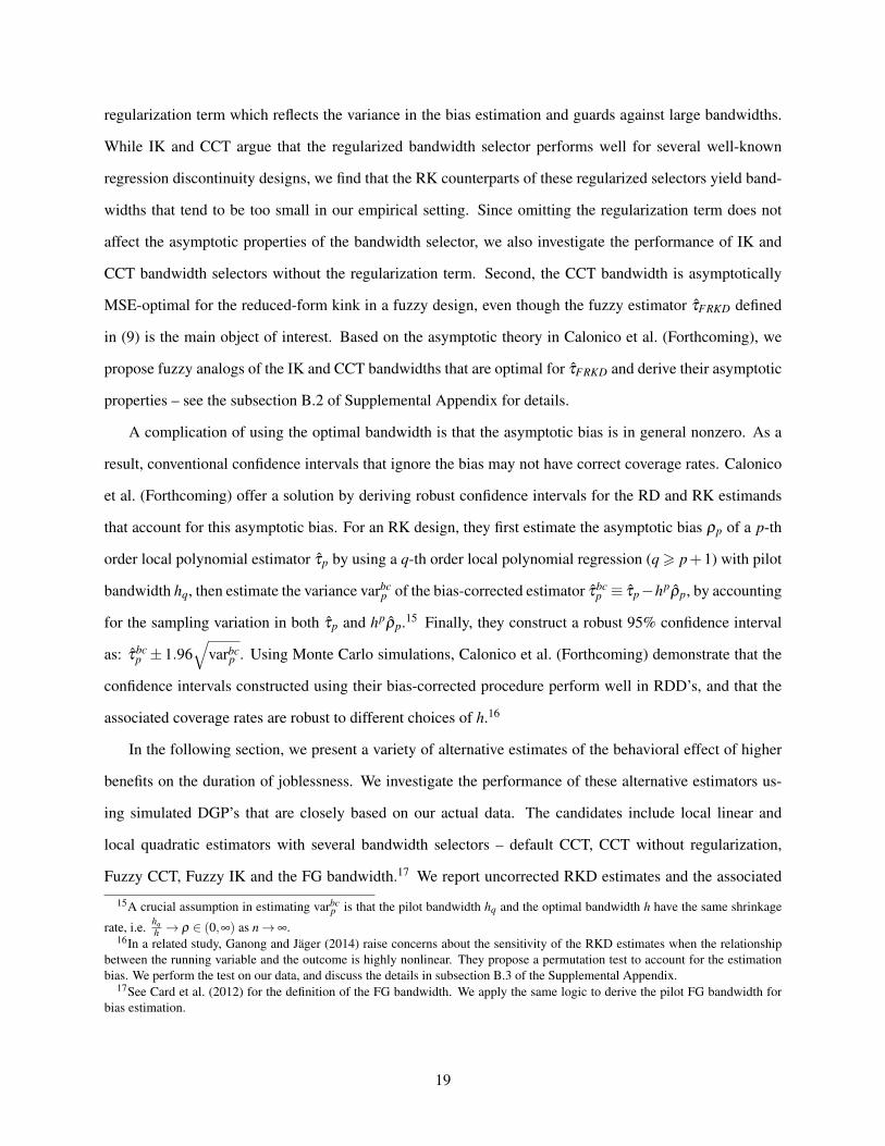
Figure 1 for our application below, the majority of the data points (B∗,V ∗) appear to lie precisely on the
benefit schedule, a feature that we interpret as evidence of a mass point at zero in the joint distribution of
(UV ,UB). Assumption 3a can be formally tested by the existence of a first-stage kink in E[B∗|V ∗ = v∗] as
stated in Remark 4 below.
Assumption 4a modifies Assumption 4: for each U = u and ε = e, there is a joint density of V and the
measurement error components that is continuously differentiable in v. Note that this allows a relatively
general measurement error structure in the sense that V,UV ′ ,UB′ can be arbitrarily correlated. Assumption 5
states that the mass point probabilities, while potentially dependent on all other variables, are smooth with
respect to V .
Assumption 6 states that the direction of the kink is either non-negative or non-positive for the entire
population, and it is analogous to the monotonicity condition of Imbens and Angrist (1994). In particular,
Assumption 6 rules out situations where some individuals experience a positive kink at V = 0, but others
experience a negative kink at V = 0. In our application below, where actual UI benefits depend on the (un-
observed) number of dependents, this condition is satisfied since the benefit schedules for different numbers
of dependents are all parallel.
Proposition 2. In a valid Fuzzy RK Design, that is, when Assumptions 1a, 2, 3a, 4a, 5 and 6 hold:
(a) Pr(U 6 u,ε 6 e|V ∗ = v∗) is continuously differentiable in v∗ at v∗ = 0 ∀(u,e) ∈ IU,ε .
(b)lim
v0→0+dE[Y |V∗=v∗ ]
dv∗
∣∣∣v∗=v0
− limv0→0−
dE[Y |V∗=v∗]dv∗
∣∣∣v∗=v0
limv0→0+
dE[B∗|V∗=v∗ ]dv∗
∣∣∣v∗=v0
− limv0→0−
dE[B∗|V∗=v∗ ]dv∗
∣∣∣v∗=v0
=∫
y1 (b(0,e) ,0,u)ϕ (u,e)dFU,ε(u,e)
where ϕ (u,e) =Pr[UV=0|V=0,U=u,ε=e](b+1 (e)−b−1 (e))
fV |U=u,ε=e(0)
fV (0)∫Pr[UV=0|V=0,ε=ω](b+1 (ω)−b−1 (ω))
fV |ε=ω(0)
fV (0) dFε (ω).
The proof is in subsection A.1 of the Supplemental Appendix.
Remark 4. The fuzzy RKD continues to estimate a weighted average of marginal effects of B on Y , but the
weight is now given by ϕ (u,e). Assumption 3a and 6 ensure that the denominator of ϕ (u,e) is nonzero.
They also ensure a kink at v∗ = 0 in the first-stage relationship between B∗ and V ∗, as seen from the proof
of Proposition 2. It follows that the existence of a first-stage kink serves as a test of Assumption 3a and 6.
Remark 5. The weight ϕ (u,e) has three components. The first component, fV |U=u,ε=e(0)fV (0)
, is analogous to
the weight in a sharp RKD and reflects the relative likelihood that an individual of type U = u,ε = e is
13

situated at the kink (i.e., has V = 0). The second component, b+1 (e)− b−0 (e), reflects the size of the kink
in the benefit schedule at V = 0 for an individual of type e. Analogously to the LATE interpretation of
a standard instrumental variables setting, the fuzzy RKD estimand upweights types with a larger kink at
the threshold V = 0. Individuals whose benefit schedule is not kinked at V = 0 do not contribute to the
estimand. An important potential difference from a standard LATE setting is that non-compliers may still
receive positive weights if the schedule they follow as non-compliers has a kink at V = 0. Finally, the
third component Pr [UV = 0|V = 0,U = u,ε = e] represents the probability that the assignment variable is
correctly measured at V = 0. Again, this has the intuitive implication that observations with a mismeasured
value of the assignment variable do not contribute to the fuzzy RKD estimand. Note that if π i j is constant
across individuals then this component of the weight is just a constant.
Remark 6. So far we have focused on a continuous treatment variable B, but the RKD framework may be
applied to estimate the treatment effect of a binary variable as well. As mentioned above, Dong (2013)
discusses the identification of the treatment effect within an RD framework where the treatment probability
conditional on the running variable is continuous but kinked. Under certain regularity conditions, Dong
(2013) shows that the RK estimand identifies the treatment effect at the RD cutoff for the group of compliers.
In practice it may be difficult to find policies where the probability of a binary treatment is statutorily
mandated to have a kink in an observed running variable. One possibility, suggested by a referee, is that the
kinked relationship between two continuous variables B and V may induce a kinked relationship between
T and V where T is a binary treatment variable of interest. In this case, we may apply the RK design to
measure the treatment effect of T . To be more specific, let
Y = y(T,V,U)
T = 1[T ∗>0] where T ∗ = t(B,V,η)
B = b(V ) is continuous in V with a kink at V = 0.
As an example, B is the amount of financial aid available, which is a kinked function of parental income
V . T ∗ is a latent index function of B, V , and a one-dimensional error term η . A student will choose to
attend college (T = 1) if T ∗ > 0. We are interested in estimating the average returns to college education,
an expectation of y(1,V,U)− y(0,V,U). Assuming that t is monotonically increasing in its third argument
and that for every (b,v) ∈ Ib(V )× IV there exists an n such that t(b(v),v,n) = 0, we can define a continuously
14

differentiable function η : Ib(V )× IV → R such that t(b,v, η(b,v)) = 0 by the implicit function theorem. We
show in subsection A.3 of the Supplemental Appendix that under additional regularity conditions, we have
the following identification result for the fuzzy RK estimand:
limv0→0+
dE[Y |V=v]dv
∣∣∣v=v0− lim
v0→0−dE[Y |V=v]
dv
∣∣∣v=v0
limv0→0+
dE[T |V=v]dv
∣∣∣v=v0− lim
v0→0−dE[T |V=v]
dv
∣∣∣v=v0
=∫
u[y(1,0,u)− y(0,0,u)]
fV,η |U=u(0,n0)
fV,η (0,n0)dFU (u) (4)
where n0 ≡ η(b0,0) is the threshold value of η when V = 0 such that n > n0⇔ T (b0,0,n) = 1. The right
hand side of equation (4) is similar to that in part (b) of Proposition 1, and the weights reflect the relative
likelihood of V = 0 and η = n0 for a student of type U .
Crucial to the point identification result above is the exclusion restriction that B does not enter the
function y as an argument, i.e. that the amount of financial aid does not have an independent effect on future
earnings conditional on parental income and college attendance. When this restriction is not met, the RK
estimand can be used to bound the effect of T on Y if theory can shed light on the sign of the independent
effect of B on Y . The details are in subsection A.3 of the Supplemental Appendix.
We can also allow the relationship between B and V to be fuzzy by writing B = b(V,ε) and introducing
measurement error in V as above. Similar to Proposition 2, we show that the fuzzy RK estimand still
identifies a weighted average of treatment effect under certain regularity assumptions. The weights are
similar to those in Proposition 2, and the exact expression is in the Supplemental Appendix.
2.3 Testable Implications of the RKD
In this section we formalize the testable implications of a valid RK design. Specifically, we show that the
key smoothness conditions given by Assumptions 4 and 4a lead to two strong testable predictions. The first
prediction is given by the following corollary of Propositions 1 and 2:
Corollary 1. In a valid Sharp RKD, fV (v) is continuously differentiable in v. In a valid Fuzzy RKD, fV ∗ (v∗)
is continuously differentiable in v∗.
The key identifying assumption of the sharp RKD is that the density of V is sufficiently smooth for
every individual. This smoothness condition cannot be true if we observe either a kink or a discontinuity
in the density of V . That is, evidence that there is “deterministic sorting” in V at the kink point implies a
violation of the key identifying sharp RKD assumption. This is analogous to the test of manipulation of the
assignment variable for RD designs, discussed in McCrary (2008). In a fuzzy RKD, both Assumption 4a, the
15

smooth-density condition, and Assumption 5, the smooth-probability-of-no-measurement-error condition,
are needed to ensure the smoothness of fV ∗ (see the proof of Lemma 5), and a kink or a discontinuity in fV ∗
indicates that either or both of the assumptions are violated.
The second prediction presumes the existence of data on “baseline characteristics” – analogous to char-
acteristics measured prior to treatment assignment in an idealized randomized controlled trial – that are
determined prior to V .
Assumption 8. There exists an observable random vector, X = x(U) in the sharp design and X = x(U,ε)
in the fuzzy design, that is determined prior to V . X does not include V or B, since it is determined prior to
those variables.
In conjunction with our basic identifying assumptions, this leads to the following prediction:
Corollary 2. In a valid Sharp RKD, if Assumption 8 holds, then d Pr[X≤x|V=v]dv is continuous in v at v = 0 for
all x. In a valid Fuzzy RKD, if Assumption 8 holds, then d Pr[X≤x|V ∗=v∗]dv∗ is continuous in v∗ at v∗ = 0 for all x.
The smoothness conditions required for a valid RKD imply that the conditional distribution function
of any predetermined covariates X (given V or V ∗) cannot exhibit a kink at V = 0 or V ∗ = 0. Therefore,
Corollary 2 can be used to test Assumption 4 in a sharp design and Assumption 4a and 5 jointly in a
fuzzy design. This test is analogous to the simple “test for random assignment” that is often conducted in a
randomized trial, based on comparisons of the baseline covariates in the treatment and control groups. It also
parallels the test for continuity of Pr[X ≤ x|V = v] emphasized by Lee (2008) for a regression discontinuity
design. Importantly, however, the assumptions for a valid RKD imply that the derivatives of the conditional
expectation functions (or the conditional quantiles) of X with respect to V (or V ∗) are continuous at the kink
point – a stronger implication than the continuity implied by the sufficient conditions for a valid RDD.
3 Nonparametric Estimation and Inference in a Regression Kink Design
In this section, we review the theory of estimation and inference in a regression kink design. We assume that
estimation is carried out via local polynomial regressions. For a sharp RK design, the first stage relationship
b(·) is a known function, and we only need to solve the following least squares problems
minβ−j
n−
∑i=1Y−i −
p
∑j=0
β−j (V
−i ) j2K(
V−ih
) (5)
16

minβ+
j
n+
∑i=1Y+
i −p
∑j=0
β+j (V
+i ) j2K(
V+ih
) (6)
where the− and + superscripts denote quantities in the regression on the left and right side of the kink point
respectively, p is the order of the polynomial, K the kernel, and h the bandwidth. Since κ+1 = limv→0+ b′(v)
and κ−1 = limv→0− b′(v) are known quantities in a sharp design, the sharp RKD estimator is defined as
τSRKD =β+1 − β
−1
κ+1 −κ
−1.
In a fuzzy RKD, the first stage relationship is no longer deterministic. We need to estimate the first-stage
slopes on two sides of the threshold by solving12
minκ−j
n−
∑i=1B−i −
p
∑j=0
κ−j (V
−i ) j2K(
V−ih
) (7)
minκ+j
n+
∑i=1B+
i −p
∑j=0
κ+j (V
+i ) j2K(
V+ih
). (8)
The fuzzy RKD estimator τFRKD can then be defined as
τFRKD =β+1 − β
−1
κ+1 − κ
−1. (9)
Lemma A1 and A2 of Calonico et al. (Forthcoming) establish the asymptotic distributions of the sharp
and fuzzy RKD estimators, respectively. It is shown that under certain regularity conditions the estimators
obtained from local polynomial regressions of order p are asymptotically normal:
√nh3(τSRKD,p− τSRKD−hp
ρSRKD,p) ⇒ N(0,ΩSRKD,p)
√nh3(τFRKD,p− τFRKD−hp
ρFRKD,p) ⇒ N(0,ΩFRKD,p)
where ρ and Ω denote the asymptotic bias and variance respectively.13 Given the identification assumptions
above, one expects the conditional expectation of Y given V to be continuous at the threshold. A natural
question is whether imposing continuity in estimation (as opposed to estimating separate local polynomials
12We omit the asterisk in B∗ and V ∗ notations in the fuzzy design to ease exposition.13In categorizing the asymptotic behavior of fuzzy estimators, both Card et al. (2012) and Calonico et al. (Forthcoming) assume
that the researcher observes the joint distribution (Y,B,V ). In practice, there may be applications where (B,V ) is observed in onedata source whereas (Y,V ) is observed in another, and the three variables do not appear in the same data set. We investigate thetwo-sample estimation problem in subsection B.1 of the Supplemental Appendix.
17

on either side of the threshold) may affect the asymptotic bias and variance of the kink estimator. Card et al.
(2012) shows that when K is uniform the asymptotic variances are not affected by imposing continuity. A
similar calculation reveals that the asymptotic biases are not affected either.
When implementing the RKD estimator in practice, one must make choices for the polynomial order p,
kernel K and bandwidth h. In the RD context where the quantities of interest are the intercept terms on two
sides of the threshold, Hahn et al. (2001) propose local linear (p = 1) over local constant (p = 0) regression
because the former leads to a smaller order of bias (Op(h2)) than the latter (Op(h)). Consequently, the local
linear model affords the econometrician a sequence of bandwidths that shrinks at a slower rate, which in
turn delivers a smaller order of the asymptotic mean-squared error (MSE). The same logic would imply that
a local quadratic (p = 2) should be preferred to local linear (p = 1) in estimating boundary derivatives in
the RK design. As we argue in Card et al. (2014), however, arguments based solely on asymptotic rates
cannot justify p = 1 as the universally preferred choice for RDD or p = 2 as the universally preferred choice
for RKD. Rather, the best choice of p in the mean squared error sense depends on the sample size and the
derivatives of the conditional expectation functions, E[Y |V = v] and E[B|V = v], in the particular data set
of interest. In Card et al. (2014), we propose two methods for picking the polynomial order for interested
empiricists: 1. evaluate the empirical performance of the alternative estimators using simulation studies
of DGP’s closely based on the actual data; 2. estimate the asymptotic mean squared error (AMSE) and
compare it across alternative estimators. Using these methods we argue in section 4 below that the local
linear estimator is a more sensible choice than the local quadratic for the Austrian UI data we study.
For the choice of K we adopt a uniform kernel following Imbens and Lemieux (2008) and the common
practice in the RD literature. The results are similar when the boundary optimal triangular kernel (c.f. Cheng
et al. (1997)) is used.
For the bandwidth choice h, we use and extend existing selectors in the literature. Imbens and Kalya-
naraman (2012) propose an algorithm to compute the MSE-optimal RD bandwidth. Building on Imbens
and Kalyanaraman (2012), Calonico et al. (Forthcoming) develop an optimal bandwidth algorithm for the
estimation of the discontinuity in the ν-th derivative, which contains RKD (ν = 1) as a special case.14
We examine alternatives to the direct analogs of the default IK and the CCT bandwidths for RKD,
addressing two specific issues that are relevant for our setting. First, both bandwidth selectors involve a
14The optimal bandwidth in Calonico et al. (Forthcoming) is developed for the unconstrained RKD estimator, i.e. withoutimposing continuity in the conditional expectation of Y , but the bandwidth is also optimal for the constrained RKD estimatorbecause it has the same asymptotic distribution as stated above.
18
regularization term which reflects the variance in the bias estimation and guards against large bandwidths.
While IK and CCT argue that the regularized bandwidth selector performs well for several well-known
regression discontinuity designs, we find that the RK counterparts of these regularized selectors yield band-
widths that tend to be too small in our empirical setting. Since omitting the regularization term does not
affect the asymptotic properties of the bandwidth selector, we also investigate the performance of IK and
CCT bandwidth selectors without the regularization term. Second, the CCT bandwidth is asymptotically
MSE-optimal for the reduced-form kink in a fuzzy design, even though the fuzzy estimator τFRKD defined
in (9) is the main object of interest. Based on the asymptotic theory in Calonico et al. (Forthcoming), we
propose fuzzy analogs of the IK and CCT bandwidths that are optimal for τFRKD and derive their asymptotic
properties – see the subsection B.2 of Supplemental Appendix for details.
A complication of using the optimal bandwidth is that the asymptotic bias is in general nonzero. As a
result, conventional confidence intervals that ignore the bias may not have correct coverage rates. Calonico
et al. (Forthcoming) offer a solution by deriving robust confidence intervals for the RD and RK estimands
that account for this asymptotic bias. For an RK design, they first estimate the asymptotic bias ρp of a p-th
order local polynomial estimator τp by using a q-th order local polynomial regression (q > p+1) with pilot
bandwidth hq, then estimate the variance varbcp of the bias-corrected estimator τbc
p ≡ τp−hpρp, by accounting
for the sampling variation in both τp and hpρp.15 Finally, they construct a robust 95% confidence interval
as: τbcp ± 1.96
√varbc
p . Using Monte Carlo simulations, Calonico et al. (Forthcoming) demonstrate that the
confidence intervals constructed using their bias-corrected procedure perform well in RDD’s, and that the
associated coverage rates are robust to different choices of h.16
In the following section, we present a variety of alternative estimates of the behavioral effect of higher
benefits on the duration of joblessness. We investigate the performance of these alternative estimators us-
ing simulated DGP’s that are closely based on our actual data. The candidates include local linear and
local quadratic estimators with several bandwidth selectors – default CCT, CCT without regularization,
Fuzzy CCT, Fuzzy IK and the FG bandwidth.17 We report uncorrected RKD estimates and the associated
15A crucial assumption in estimating varbcp is that the pilot bandwidth hq and the optimal bandwidth h have the same shrinkage
rate, i.e. hqh → ρ ∈ (0,∞) as n→ ∞.
16In a related study, Ganong and Jäger (2014) raise concerns about the sensitivity of the RKD estimates when the relationshipbetween the running variable and the outcome is highly nonlinear. They propose a permutation test to account for the estimationbias. We perform the test on our data, and discuss the details in subsection B.3 of the Supplemental Appendix.
17See Card et al. (2012) for the definition of the FG bandwidth. We apply the same logic to derive the pilot FG bandwidth forbias estimation.
19

(conventional) sampling errors associated with each polynomial order and bandwidth choice, as well as
bias-corrected estimates and the associated robust confidence intervals suggested by Calonico et al. (Forth-
coming).18
4 The Effect of UI Benefits on the Duration of Joblessness
In this section, we use a fuzzy RKD approach to estimate the effect of higher unemployment benefits on the
duration of joblessness among UI claimants in Austria. The precise magnitude of the disincentive effect of
UI benefits is of substantial policy interest. As shown by Baily (1978), for example, an optimal unemploy-
ment insurance system trades off the moral hazard costs of reduced search effort against the risk-sharing
benefits of more generous payments to the unemployed.19 Obtaining credible estimates of this effect is diffi-
cult, however, because UI benefits are determined by previous earnings, and are likely to be correlated with
unobserved characteristics of workers that affect both wages and the expected duration of unemployment.
Since the UI benefit formula in Austria has both a minimum and maximum, a regression kink approach can
provide new evidence on the impact of higher UI benefits at two different points in the benefit schedule. We
begin with a brief discussion of a job search model that we use to frame our analysis. We then describe the
benefit system in Austria, our data sources, and our main results.
4.1 Theoretical background
In a standard search model, higher UI benefits reduce the incentives for search and raise the reservation wage,
leading to increases in the expected duration of joblessness. Higher benefits can also affect the equilibrium
distribution of wages. Christensen et al. (2005), for example, derive the equilibrium distribution of wages,
given a fixed UI benefit and a latent distribution of wage offers. In their model, a twice continuously
differentiable distribution function for wage offers ensures that distribution of wages among newly laid-off
workers is twice continuously differentiable. In section C of the Supplemental Appendix we extend this
model to incorporate a UI benefit schedule that is linear in the previous wage up to some maximum T max.
In this case the value function of unemployed workers is increasing in their previous wage with a a kink at
T max. Likewise, the value function associated with a job paying a wage w has a kink at w = T max, reflecting18Even though τbc
p is not consistent under the CCT asymptotic assumptions regarding the shrinkage rate of hq and h, it may stillbe informative to report its value and shed light on the direction and magnitude of the estimated bias.
19The original analysis in Baily (1978) has been generalized to allow for liquidity constraints (Chetty (2010)) and variable takeup(Kroft (2008)).
20

the kink in the option value of UI benefits when the job ends. This kink causes a kink in the relationship
between wages and on-the-job search effort which leads to a kink in the density of wages at T max (see the
Supplemental Appendix for details). Assuming a constant rate of job destruction there is a similar kink in
the density of previous wages among job-losers. Such a kink – at precisely the threshold for the maximum
benefit rate – violates the smooth density condition (i.e., Assumptions 4/4a) necessary for a valid regression
kink design based on the change in the slope of the benefit function at T max.20 Nevertheless, we also show
that if workers have some uncertainty about the location of the kink in future UI benefits, the equilibrium
density of previous wages among job losers will be smooth at T max.
Given these theoretical possibilities, it is important to examine the actual distribution of pre-displacement
wages among job seekers and test for the presence of kinks around the minimum and maximum benefit
thresholds, as well as for kinks in the conditional distributions of predetermined covariates. While we do
not necessarily expect to find kinks in our setting (given the difficulty of forecasting future benefit schedules
in Austria), a kink could exist in other settings where minimum or maximum UI benefits are often fixed for
several years at the same nominal value.
4.2 The Unemployment Insurance System in Austria
Job-losers in Austria who have worked at least 52 weeks in the past 24 months are eligible for UI benefits,
with a rate that depends on their average daily earnings in the “base year” for their benefit claim, which
is either the previous calendar year, or the second most recent year. The daily UI benefit is calculated as
55% of net daily earnings, subject to a maximum benefit level that is adjusted each year. Claimants with
dependent family members are eligible for supplemental benefits based on the number of dependents. There
is also a minimum benefit level for lower-wage claimants, subject to the proviso that total benefits cannot
exceed 60% (for a single individual) or 80% (for a claimant with dependents) of base year net earnings.
These rules create a piecewise linear relationship between base year earnings and UI benefits that de-
pends on the Social Security and income tax rates as well as the replacement rate and the minimum and
maximum benefit amounts. To illustrate, Figure 1 plots actual daily UI benefits against annual base year
earnings for a sample of UI claimants in 2004. The high fraction of claimants whose observed UI benefits
20In the model as written all workers are identical: hence a kink in the density of wages at T max will not actually invalidate anRK design. More realistically, however, workers differ in their cost of search (and in other dimensions) and the kink at T max islarger for some types than others, causing a discontinuity in the conditional distribution of unobserved heterogeneity at T max thatleads to bias in an RKD.
21

are exactly equal to the amount predicted by the formula leads to a series of clearly discernible lines in the
figure, though there are also many observations scattered above and below these lines.21 Specifically, in the
middle of the figure there are 5 distinct upward-sloping linear segments, corresponding to claimants with 0,
1, 2, 3, or 4 dependents. These schedules all reach an upper kink point at the maximum benefit threshold
(which is shown in the graph by a solid vertical line). At the lower end, the situation is more complicated:
each of the upward-sloping segments reaches the minimum daily benefit at a different level of earnings,
reflecting the fact that the basic benefit includes family allowances, but the minimum does not. Finally,
among the lowest-paid claimants the benefit schedule becomes upward-sloping again, with two major lines
representing single claimants (whose benefit is 60% of their base earnings, net of taxes) and those with
dependents (whose benefits are 80% of their net base year earnings).22
Our RKD analysis exploits the kinks induced by the minimum and maximum benefit levels. Since we do
not observe the number of dependents claimed by a job loser, we adopt a fuzzy RKD approach in which the
number of dependents is treated as an unobserved determinant of benefits. This does not affect the location
of the “top kink” associated with the maximum benefit, since claimants with different numbers of dependents
all have the same threshold earnings level T max for reaching the maximum. For the “bottom kink” associated
with the minimum benefit, we define T min as the kink point for a single claimant: this is the level of annual
earnings shown in the figure by a solid vertical line. To the right of T min the benefit schedules for all
claimant groups are upward-sloping. To the left, benefits for claimants with no dependents are constant,
whereas benefits for claimants with dependents continue to fall. Thus we expect to measure a kink in the
average benefit function at T min that is proportional to the fraction of claimants with no dependents. We
limit our analysis to claimants whose earnings are high enough to avoid the “subminimum” portion of the
benefit schedule: this cutoff is shown by the dashed line on the left side of Figure 1. We also focus on
claimants whose annual earnings are below the Social Security contribution cap, since earnings above this
level are censored. This cutoff is shown by the dashed line on the right side of Figure 1.
21These are attributable to some combination of errors in the calculation of base year earnings (due to errors in the calculation ofthe claim start date, for example), errors in the Social Security earnings records that are over-ridden by benefit administrators, andmis-reported UI benefits. Similar errors have been found in many other settings – e.g., Kapteyn and Ypma (2007).
22The line for low-earning single claimants actually bends, reflecting the earnings threshold at which a single claimant beginspaying income taxes.
22

4.3 Data and Analysis Sample
Our data are drawn from the Austrian Social Security Database (ASSD), which records employment and
unemployment spells on a daily basis for all individuals employed in the Austrian private sector (see
Zweimüller et al. (2009)). The ASSD contains information on starting and ending dates of spells and
earnings (up to the Social Security contribution cap) received by each individual from each employer in a
calendar year. We merge the ASSD with UI claims records that include the claim date, the daily UI benefit
actually received by each claimant, and the duration of the benefit spell. We use the UI claim dates to assign
the base calendar year for each claim, and then calculate base year earnings for each claim, which is the
observed assignment variable for our RKD analysis (i.e., V ∗ in the notation of section 2). In addition, we
observe the claimant’s age, gender, education, marital status, job tenure, and industry. Our main outcome
variable is the time between the end of the old job and the start of any new job (which we censor at 1 year).
Our analysis sample includes claimants from 2001-2012 with at least one year of tenure on their previous
job who initiated their claim within four weeks of the job ending date (eliminating job-quitters, who face
a four-week waiting period). We drop people with zero earnings in the base year, claimants older than
50, and those whose earnings are above the Social Security earnings cap or so low that they fall on the
“subminimum” portion of the benefit schedule. We pool observations from different years as follows. First,
we divide the claimants in each year into two (roughly) equal groups based on their gross base year earnings:
those below the 50th percentile are assigned to the “bottom kink” sample, while those above this threshold
are assigned to the “top kink” sample. Since earnings have a right-skewed distribution, the cutoff threshold
is closer to T min than T max, implying a narrower support for our observed assignment variable V ∗ (observed
annual base year earnings) around the bottom kink than the top kink. Next we re-center base year earnings
for observations in the bottom kink subsample around T min , and base year earnings for those in the top kink
subsample around T max, so both kinks occur at V ∗ = 0. Finally, we pool the yearly re-centered subsamples
into bottom and top kink samples, yielding about 275,000 observations in each sample.
Table 1 reports basic summary statistics for the bottom and top kink samples. Mean base year earnings
for the bottom kink group are about C22,000, with a relatively narrow range of variation (standard deviation
= C2,800), while mean earnings in the top kink group are higher (mean = C34,000) and more dispersed
(standard deviation = C6,700). Mean daily UI benefits are C25.2 for the bottom kink group (implying an
annualized benefit of C9,200, about 44% of T min), while mean benefits for the top kink sample are C33.5
23

(implying an annualized benefit of C12,300, about 28% of T max). Claimants in the bottom kink sample are
more likely to be female, are a little younger, less likely to be married, more likely to have had a blue-collar
occupation, and are less likely to have post-secondary education. Despite the differences in demographic
characteristics and mean pay, the means of the main outcome variable are quite similar in the two samples:
the average duration of joblessness is around 150 days. Only about 10 percent of claimants exhaust their
regular UI benefits.
A key assumption for valid inference in an RK design is that the density of the assignment variable (in
our case, base year earnings) is smooth at the kink point. Figures 2a and 2b show the frequency distributions
of base year earnings in our two subsamples, using 100-Euro bins for the bottom kink sample and 300-Euro
bins for the top kink sample (each with about 4,200 observations per bin). While the histograms look quite
smooth, we tested this more formally by fitting a series of polynomial models that allow the first and higher-
order derivatives of the binned density function to jump at the kink point.23 We test for a kink by testing
for a jump in the linear term of the polynomial at the kink. Appendix Table 1 shows the goodness of fit and
Akaike model selection statistics for polynomial models of order 2, 3, 4, or 5, as well as the estimated kinks
at T min and T max. We show the fitted values from the models with the lowest Akaike criterion – a 3rd order
model for the bottom kink sample and a 4th order model for the top kink sample – in Figures 2a and 2b. In
both cases the fitted densities appear to be quite smooth.
4.4 Graphical Overview of the Effect of Kinks in the UI Benefit Schedule
As a starting point for our RKD analysis, Figures 3 and 4 show the relationships between base year earnings
and actual UI benefits around the bottom and top kinks. We plot the data using the same bin sizes as in
Figures 2a and 2b.24 The Figures show clear kinks in the empirical relationship between average benefits
and base year earnings, with a sharp increase in slope as earnings pass through the lower threshold T min and
a sharp decrease as they pass through the upper threshold T max.25 Figures 5 and 6 present parallel figures for
the mean log time to the next job. These figures also show discernible kinks, though there is clearly more
variability in the relationship with base year earnings.
23We use a minimum chi-squared objective, which Lindsay and Qu (2003) show can be interpreted as a optimally weightedminimum distance objective for the multinomial distribution of histogram frequencies.
24See Calonico et al. (2014a) for nonparametric procedures for picking the bin size in RD-type plots.25The slopes in the mean benefit functions to the left of T min and to the right of T maxare mainly attributable to family allowances.
Moving left from T min the average number of dependent allowances is falling, as claimants with successively higher numbers ofdependents hit the minimum benefit level (see Figure 1). Likewise, moving right from T max the average number of allowances isrising, reflecting a positive correlation between earnings and family size.
24

Given the relatively short duration of UI benefits in our sample (20 - 39 weeks), it is also interesting to
look at the probability a claimant exhausts benefits. Appendix Figure 1a shows this probability around the
bottom kink. The discrete increase in the slope with respect to base year earnings suggests that higher UI
benefits increase the probability of exhaustion. Appendix Figure 1b presents a parallel graph around the top
kink. The exhaustion probability exhibits a kink in the expected direction, though as with our main outcome
variable, the probabilities are relatively noisy in the range of earnings just above T max.
Finally, we examine the patterns of the predetermined covariates around T min and T max. Appendix Fig-
ures 2 and 3 show the conditional means of four main covariates around the two kink points: age, gender,
blue-collar occupation, and an indicator for whether the claimant had been recalled to the previous job.26
The graphs show some evidence of non-smoothness in the conditional means of the covariates in the bottom
kink sample, particularly for claimant age. To increase the power of this analysis we constructed a “covari-
ate index” – the predicted duration of joblessness from a simple linear regression model relating the log of
time to next job to a total of 59 predetermined covariates, including gender, occupation, age, previous job
tenure, quintile of the previous daily wage, industry, region, year of the claim, previous firm size, and the
recall rates of the previous employer.27 This estimated covariate index function can be interpreted as the
best linear prediction of mean log time to next job given the vector of predetermined variables.
Figures 7 and 8 plot the mean values of the estimated covariate indices around the top and bottom kinks.
Visually, the predicted time to next job appears to evolve relatively smoothly through both the top and
bottom kinks. In the next subsection, we provide a more formal comparison of the estimated slopes of the
conditional mean functions for the covariate indices.
4.5 RKD Estimation Results
4.5.1 Reduced Form Kinks in Assignment and Outcome Variables
Table 2a presents reduced form estimates of the kinks in our endogenous policy variable (log daily benefits)
and our main outcome variable (log of time to next job) around T min and T max. For each variable we show
results using three different bandwidth selection procedures: the default CCT procedure; the CCT bandwidth
selection procedure without regularization; and the FG bandwidth. We show the estimated kink arising from
26Many seasonal jobs in Austria lay off workers at the end of the season and re-hire them again at the start of the next season.Having been recalled from unemployment to the recently lost job is a good indicator that the present spell may end with recall tothat job again – see Del Bono and Weber (2008).
27We fit a single prediction model using the pooled bottom kink and top kink samples.
25

each selected bandwidth, as well as the corresponding bias-corrected estimate and the associated robust 95%
confidence interval.28 We present estimates from local linear models in columns 1 and 3, and from local
quadratic models in columns 2 and 4.
Despite the strong visual evidence of kinks in the benefit formula in Figures 3 and 4, an examination of
the estimated “first stage” kinks in Panel A of Table 2 suggests that not all the procedures yield statistically
significant kink estimates. In particular, the default CCT bandwidth selector chooses relatively small band-
widths for the local linear model and yields an insignificant estimate of the bottom kink (t = 1.7) and only
a marginally significant estimate of the top kink (t = 2.1). The corresponding bias-corrected kink estimates
are substantially less precise, with sampling errors about 40% larger than the uncorrected estimates. Al-
though the default CCT procedure chooses somewhat larger bandwidths for the local quadratic models, this
is offset by the difficulty of precisely estimating the slopes on either side of the kink point once the quadratic
terms are included, and neither the estimated bottom kink or the estimated top kink in the quadratic mod-
els is close to significant. As with the local linear models, the corresponding bias-corrected quadratic kink
estimates are even less precise, with very wide confidence intervals.
Relative to the default CCT bandwidth selector, the CCT selector without regularization yields substan-
tially larger bandwidths – over 2 times larger for the local linear models, and 30-50% larger for the local
quadratic models. These larger bandwidths yield uncorrected first stage kink estimates from the local linear
models that are relatively precise (t > 10 for the bottom kink sample, t = 6 for the top kink sample). The es-
timated kinks from the local quadratic estimates, however, are still relatively noisy, as are the bias-corrected
estimates from either the local linear or local quadratic models. By comparison the bandwidths selected
by the FG procedure are relatively large, and deliver seven significant first stage estimates in eight cases.
Interestingly, a comparison of the uncorrected and bias-corrected estimates from the FG selection procedure
suggests that the biases associated with the naive FG bandwidth choice are relatively small, except in the
case of the local quadratic estimate for the top kink.
Turning to the reduced form outcome models in Panel B, the estimated kinks in the duration of jobless-
ness are less precisely estimated than the kinks in log benefits. Again, the default CCT bandwidth selector
chooses relatively small bandwidths and yields very noisy estimates of the kink. The bandwidths under the
CCT procedure without the regularization term are substantially larger, and yield marginally significant es-
28Robust confidence intervals and the CCT bandwidths are obtained based on a variant of the Stata package described in Calonicoet al. (in press) with the nearest-neighbor variance estimator, which we also use in the simulations below. Using the CCT Statapackage generates very similar empirical estimates.
26

timated kinks in the outcome variable from the local linear models. The FG bandwidths are even larger, and
yield estimated kinks that are significant or marginally significant in both the linear and quadratic models.
The bias-corrected estimates are in all but one case insignificant, however, reflecting the additional uncer-
tainty associated with the bias correction term.29 Interestingly, the bias-corrected local linear estimates for
the bottom and top kink are both larger in absolute value than the corresponding uncorrected estimates,
suggesting that the uncorrected estimates may be conservative. Finally, as we found with the first stage kink
estimates, the local quadratic estimates in the reduced form model are quite imprecise, and the bias-corrected
local quadratic models are essentially uninformative.
In finite samples, the use of higher order polynomial models and bias correction may come at the cost
of an increase in variance relative to lower-order uncorrected models. In the remainder of this section we
examine the tradeoff between bias and variance associated with the CCT bias correction procedure. We
defer a discussion of the polynomial order choice to subsection 4.5.3. As mentioned in section 3, the intent
of CCT’s bias correction is to eliminate the bias in the p-th order polynomial estimator τp by subtracting off
the estimated asymptotic bias, hpρp. The cost of bias correction, however, is that the bias term is imprecisely
estimated, leading to a potential increase in the overall variance of the corrected estimator τbcp relative to the
uncorrected estimator τp.30 The usual metric for trading off bias and variance is the (asymptotic) mean
squared error of the estimator, which is the sum of its squared bias and its variance. By Lemma A1 and
Theorem A1 of Calonico et al. (Forthcoming), the asymptotic mean squared errors of τp and τbcp+1 are
AMSE(τp) = (hpρp)2 +op(h2p)+ var(τp) and AMSE(τbc
p ) = op(h2p)+varbcp . It follows that the change in
the AMSE associated with bias correction is asymptotically −(hpρp)2 +varbc
p − var(τp).
In Table 2b, we report the estimated bias hpρp, its square, and the change in estimated variance, varbcp −
var(τp), for the first stage and reduced form estimators presented in Table 2a. The increase in variance is
larger than the estimated squared bias for both the local linear and local quadratic estimates using either the
default CCT bandwidth selector, or the alternative version that ignores the regularization term. This is also
the case for the FG bandwidth in the bottom kink sample. In the top kink sample, however, the estimated
bias for the FG bandwidth is quite large, and bias correction appears to decrease the AMSE. This suggests
that bias correction could be important for estimators based on the FG bandwidth in the top kink sample. At
29The one exception is the bias-corrected local linear estimate for the top kink sample. In this case, the robust confidence intervalis relatively wide but the bias-corrected point estimate is also relatively large in magnitude.
30Remark 5 of Calonico et al. (Forthcoming) states that the variance of τbcp is smaller than that of τp for a large n, but this
asymptotic advantage may not materialize in a given finite sample, and does not appear to hold in our samples.
27

the same time, since the bias term is estimated, it may deviate from the actual bias. So in section 4.5.3, we
evaluate the performance of the various estimators in Monte Carlo simulations using DGP’s approximating
our data, where we can directly obtain the mean squared errors without having to estimate the bias.
4.5.2 Kinks in Conditional Means of Predetermined Covariates
As discussed in subsection 2.3, a key implication of the smooth density assumption underlying a valid RK
design is that the conditional distributions of any pre-determined covariates should evolve smoothly around
the kink points in the observed running variable. In the context of our UI example, this means that the
conditional means of all pre-determined claimant characteristics should vary smoothly with base-period
earnings around the bottom and top kink points. Table 3 presents tests of this smoothness prediction for the
covariate index introduced in Figure 7 and 8, as well as for the four main sub-components of this index. We
show estimated kinks from local linear and local quadratic models using the FG bandwidth selector, as well
as the corresponding bias-corrected kink estimates (and robust 95% confidence intervals).
For the bottom kink sample (Panel A), the estimates point to some reason for concern. In particular,
the conditional mean of the predicted mean of joblessness exhibits a positive kink at T min about 30% as
large as the kink in actual log time to next job (comparing the estimated kink of 0.9 for predicted log time
to the estimate of 3.0 for log actual time in Table 2a from a local linear model using the FG bandwidth).
Looking at the individual covariates, there are relatively large kinks in the conditional means of age and the
indicator for blue collar status. These kinks are visually evident in Appendix Figures 2a and 2c, and suggest
that the conditional distribution of the observed characteristics of claimants with earnings around T min is
not smooth. Given this situation, we have to interpret the estimated parameters derived from the bottom
kink sample carefully, acknowledging that there is a likely upward bias in the RKD estimate of the elasticity
of the duration of joblessness with respect to UI benefits, driven by the non-smoothness in the observed
determinants of joblessness durations.
For the top kink sample (Panel B) there is less evidence of non-smoothness, though we note that the
bias-corrected local linear model and the local quadratic models point to a possible negative kink in the
predicted log time to next job. Taken together with the relatively smooth patterns in Figure 8 and Appendix
Figures 3a-3d, however, we believe that the assumptions for a valid regression kink are plausibly satisfied
around the top kink.
28

4.5.3 Fuzzy RKD Estimates and Comparison of Alternative Estimators
As a final step in our empirical analysis we present fuzzy RKD estimates of the elasticity of the duration of
joblessness with respect to the level of UI benefits and evaluate the performance of alternative estimators.
As noted in subsections 2.2.2 and 4.2, the fuzzy RK estimand in the bottom kink sample identifies the
behavioral response for claimants whose baseline earnings are close to T min and who follow the benefit
schedule intended for single claimants. In the top kink sample, the fuzzy RK estimand identifies the elasticity
for claimants close to T max who follow any of the benefit schedules seen in Figure 1. Therefore, applying a
regression kink approach to the two samples allows us to estimate the elasticity of joblessness with respect
to UI benefit generosity for two very different subpopulations.31 Table 4 presents estimated elasticities for
the local linear and quadratic estimators under the FG bandwidth. We show both the conventional estimates
(columns 2 and 5) and the bias-corrected estimates (columns 3 and 6) with robust confidence intervals that
take account of the sampling variability of the bias corrections. Without bias correction, the local linear
models yield estimated elasticities of 1.4 and 2.0 for the bottom kink and top kink samples, respectively. In
both cases, the corresponding bias-corrected estimates are larger in magnitude, as are the estimates from the
local quadratic models, suggesting that if anything, the uncorrected local linear estimates are “conservative”.
In Table 5, we present elasticities along with first-stage estimates for four alternative bandwidth selec-
tion procedures. The alternatives we consider are: default CCT, CCT with no regularization, Fuzzy CCT
and Fuzzy IK. (Expressions for the latter two bandwidths are given in subsection B.2 of the Supplemental
Appendix). For each bandwidth selector we present the value of the main and pilot bandwidth (the pilot
bandwidth is for bias estimation in constructing the CCT confidence interval), the uncorrected and bias-
corrected first stage kink estimates, and the uncorrected and bias-corrected structural elasticities. The first
stage kink estimates are generally similar to the estimates presented in Panel A of Table 2a, but they are
not identical because the bandwidths in Table 5 are selected to be optimal for the numerator of the RKD
estimand, or for the estimand itself (in the case of the fuzzy CCT and fuzzy IK procedures) rather than for
the first stage equation.
The pattern of estimates in Table 5 point to three main conclusions. First, as we noted in the discussion
of Table 2a, many of the bandwidth selectors choose relatively small bandwidths that lead to relatively im-
31It may be tempting to apply a sharp RK design to only the observations that lie on the UI schedule. However, this approach doesnot in general identify an interpretable treatment effect, just as an analysis of the subset of “compliers” in a randomized experimentis likely to be highly problematic.
29

precise first-stage and structural coefficient estimates. A second observation is that, as in Table 2a, the local
quadratic estimators are generally quite noisy. Third, the bias-corrected estimates from the local linear mod-
els are typically not too different from the uncorrected estimates, but the added imprecision associated with
uncertainty about the magnitude of the bias correction factor is large, leading to relatively wide confidence
intervals for the bias corrected estimates.
Given the wide range of estimates in Tables 4 and 5, which specification should we pick? The line of
argument advanced in Calonico et al. (Forthcoming) suggests that one might prefer the bias-corrected esti-
mates from local quadratic models using the CCT bandwidth selector with regularization. In our application,
these estimates are imprecise. For the bottom kink sample this choice suggests the elasticity of joblessness
with respect to UI benefits is 19.0 whereas for the top kink sample the estimate is wrong-signed and equal
to -6.9. However, given the wide confidence intervals both estimates are essentially uninformative. At the
opposite extreme, the uncorrected estimates from local linear specifications using the FG bandwidth selector
(in Table 4) are relatively precisely determined and point to behavioral elasticities in the range of 1 to 2.
To gain additional insight, we decided to conduct a series of Monte Carlo simulations based on DGP’s
that closely resemble our actual samples. Because we are interested in the power of the candidate estimators,
we impose the first-stage kink parameter and the elasticity parameter in constructing the DGP’s. For the
bottom kink sample, we impose the first-stage kink as τB = 2.3× 10⁻⁵ and the elasticity τFRKD = 1.3,
which implies a reduced-form kink of τY = τB · τFRKD = 3.0× 10⁻⁵. For the top kink sample, we set
τB = −1.4× 10⁻⁵ and τFRKD = 2.0 with an implied τY = −2.8× 10⁻⁵. We then specify the DGP’s for
E[B|V ] and E[Y |V ] as separate quintics on each side of the threshold, where the parameters of the quintics
are estimated by regressing, respectively, B− τB ·D ·V and Y − τY ·D ·V on the polynomial terms V j and
D ·V k where D = 1[V>0], j = 0,1...,5 and k = 2, ...,5. For our simulation, we sample V from its empirical
distribution and the errors (εB, εY ) jointly from the residuals from the quintic regressions, and construct
B = E[B|V ]+ εB and Y = E[Y |V ]+ εY . We draw 1,000 repeated samples in our Monte Carlo exercise.
Tables 6a and 6b summarize the performance of the alternative estimators for the simulated bottom kink
and top kink samples, respectively. The two polynomial orders (linear and quadratic), two bias-correction
choices (uncorrected and bias-corrected) and six bandwidth selection procedures (default CCT, CCT with
no regularization, Fuzzy CCT, Fuzzy IK, FG, and Global) give rise to 24 candidate estimators in total. For
each estimator, we report the associated bandwidth(s) and its performance in estimating the first-stage and
the elasticity parameters.
30

The two main criteria for evaluating estimator performance are (1) the root mean squared error (RMSE)
of the elasticity estimator; and (2) how often its confidence interval covers the true parameter τFRKD. In
column (6) and (7) we report two measures of RMSE. Column (6) shows the raw RMSE as a ratio of the
imposed τFRKD. Because we worry that outliers may drive the numbers in column (6), we report in column
(7) a “trimmed” RMSE ratio by first discarding 5% of the simulation sample with the greatest deviation
between τFRKD and τFRKD. In column (8), we report the coverage rates of the confidence interval.
As seen from Table 6, none of the estimators consistently achieves the lowest RMSE and delivers the
correct coverage rate, but the conventional local linear estimator with the FG bandwidth (LLFG for short)
appears to be a reasonable choice. In the bottom kink sample, this estimator and the global conventional
linear estimator outperform all other candidates, and the two are very similar in terms of their RMSE’s and
coverage rates (96% and 94% respectively). In the top kink sample, the LLFG estimator has the smallest
RMSE, although the coverage rate of the corresponding confidence interval is a lower 82%. The lower
coverage rate is indicative of the bias of the LLFG estimator, but the bias is quite small in magnitude
(0.11) as compared to the imposed elasticity (2.0). A viable alternative for the top kink sample is the local
linear estimator with the fuzzy IK bandwidth (LLIK for short): it has a moderately higher RMSE, but the
corresponding confidence interval has a better coverage rate of 94% than LLFG. As shown in Table 5, using
LLIK also points to a statistically significant high elasticity, which is consistent with the LLFG result.
Analogously to Table 2b, we also break down the (trimmed) MSE and report the bias, squared bias
and variance of each of the estimators in columns (9)-(11) of Table 6. Bias correction appears to increase
both the squared bias and the variance for all estimators in the bottom kink simulations and for 8 out of 12
estimators in the top kink simulations. In 23 out of the 24 cases, bias correction increases the (trimmed)
RMSE, with the only exception being the global quadratic estimator for the top kink.
In a parallel simulation study, we assess the performance of the estimators in DGP’s where we impose
the true elasticity τFRKD to be zero: the results are presented in Appendix Table 2. In terms of RMSE, the FG
bandwidth still outperforms the four local alternatives, and within each bandwidth choice, the conventional
linear estimator dominates the other three candidates. In terms of the coverage rate of the corresponding 95%
confidence interval, however, LLFG no longer performs well: the coverage rate is 2% for the bottom kink
simulation and 20% for the top. Moreover, there does not appear to be an attractive alternative estimator:
those with a coverage rate above 90% have a variance at least 30 times higher than LLFG in the top kink
sample and at least 80 times higher in the bottom kink sample.
31

The poor coverage rates of the LLFG confidence interval in Appendix Table 2 raise the concern that the
structural elasticities arising from applying this procedure to our actual data may be misleading. However,
the value of the bias-corrected LLFG estimator is higher than the conventional LLFG estimator in our actual
data (1.95 versus 1.37 for the bottom kink; 3.67 versus 2.04 for the top kink), and this empirical regularity
is matched by the DGP’s underlying Table 6 but not by the DGP’s underlying Appendix Table 2. Therefore,
we believe that the simulation DGP’s underlying Table 6, as opposed to those underlying Appendix Table 2,
are better approximations to the actual data.
In another exercise, we provide further evidence that the local linear estimator should be preferred to the
local quadratic by directly estimating the AMSE’s for the local linear and quadratic estimators, per Card et
al. (2014). As shown in Appendix Table 3, using the default CCT bandwidth selection procedure the AMSE
for the local quadratic model is at least an order of magnitude larger than the AMSE for the local linear
model.32 For the other bandwidth choices, the linear AMSE is also much smaller (at least 68% smaller)
than the quadratic AMSE and we omit them from Appendix Table 3 for ease of exposition.
As a final robustness check, we investigate how sensitive the elasticity estimates are with respect to the
choice of bandwidth. Figures 9 and 10 plot the elasticity estimates for the bottom and top kink samples
associated with a range of potential bandwidths. Ruppert (1997) argues that one can use the relationship
between the point estimates and the bandwidth choice as an indicator of potential bias, with stability in the
estimate indicating the absence of significant bias. Figure 9 shows that the estimated elasticity of time to
next job with respect to UI benefits around the bottom kink is relatively stable at close to 1.4 for a very
wide range of bandwidths. Figure 10 shows that the estimated elasticity around the top kink is a little
more sensitive to bandwidth choice, with a larger estimate (between 2 and 3) for lower bandwidths, but an
elasticity of 2 or less for bandwidths above C5,000.
Overall, we conclude that the conventional local linear estimator with the FG bandwidth does reasonably
well for our empirical application. The corresponding estimates lead us to two main findings. First, for job-
losers from the upper part of the earnings distribution (around T max), the elasticity of the time to next job
with respect to UI benefits is around 2. Our confidence in this estimate is strengthened by the fact that tests
for the validity of an RK design around the top kink show little evidence that the design is compromised by
sorting.
32Note that the estimated bias component for the local quadratic estimator is substantially larger than its local linear counterpart,even though the former shrinks to zero at a faster rate.
32

A second, more tentative conclusion is that the corresponding elasticity for job-losers in the lower part
of the earnings distribution (around T min) is of a smaller magnitude – perhaps closer to 1. Our cautious
assessment stems from the fact that the tests for the validity of an RKD approach show that the conditional
distributions of observed worker characteristics change slopes around T min. These changes are not associ-
ated with any discernible “bunching” at the kink point in the benefit schedule, but they are large enough to
cause a 30% upward bias in the estimated jobless elasticity.
How do our estimated benefit elasticities compare to those in the existing literature? Appendix Table 4
contains a brief summary of the existing literature, drawing on the survey by Krueger and Meyer (2002) for
the earlier U.S.-based literature, all of which use administrative records on unemployment insurance claims
and estimate the effect of UI benefits on the duration of the initial spell of insured unemployment. These
studies point to a benefit elasticity in the range of 0.3 to 0.8.33 A recent study by Landais (Forthcoming)
applies a regression kink design to some of the same data used in these earlier studies and obtains estimates
of the elasticity of the initial UI benefit spell that range from 0.20 to 0.70. Another recent study by Chetty
(2010) uses retrospective interview data from the Survey of Income and Program Participation and obtains
an average benefit elasticity of about 0.5. Taken together these U.S. studies suggest a benchmark of around
0.5 for the elasticity of initial UI claim duration on the UI benefit. Most of the European studies included
in Appendix Table 4 estimate the effect of benefits on the time to first exit from the UI system, and obtain
benefit elasticities that are similar to the U.S. studies. An exception is Carling et al. (2011), who study the
effect of a reduction in the benefit replacement rate in Sweden in 1996 on the exit rate from unemployment
recipiency to employment. Their estimate of the elasticity of time to next job with respect to the benefit
level is 1.6, which is not far from our point estimate of 2.0 for the top kink sample.
In Card et al. (2012), we argued that the high elasticity we find may be a consequence of using time
to next job as an outcome measure as opposed to the insured unemployment duration typically used in the
literature. Our findings underscore the potential value in being able to measure time to next job in assessing
the incentive effects of the UI system.
33Krueger and Meyer attribute an estimated elasticity of 1.0 to Solon (1985) who studies the effect of making UI benefits taxableon the unemployment duration of high-earning claimants. He finds that the introduction of taxation caused a 22% reduction in theaverage duration of initial UI claims by higher-earning claimants (with no effect on low-earners). Assuming an average tax rate of30%, this implies an elasticity of 0.73, which is our preferred interpretation of Solon (1985)’s results.
33

5 Conclusion
In many institutional settings a key policy variable (like unemployment benefits or public pensions) is set
by a deterministic formula that depends on an endogenous assignment variable (like previous earnings).
Conventional approaches to causal inference, which rely on the existence of an instrumental variable that
is correlated with the covariate of interest but independent of underlying errors in the outcome, will not
work in these settings. When the policy function is continuous but kinked (i.e., non-differentiable) at a
known threshold, a regression kink design provides a potential way forward (Guryan (2001); Nielsen et
al. (2010); Simonsen et al. (Forthcoming)). The sharp RKD estimand is simply the ratio of the estimated
kink in the relationship between the assignment variable and the outcome of interest at the threshold point,
divided by the corresponding kink in the policy function. In settings where there is incomplete compliance
with the policy rule (or measurement error in the actual assignment variable), a “fuzzy RKD” replaces
the denominator of the RKD estimand with the estimated kink in the relationship between the assignment
variable and the policy variable.
In this paper we provide sufficient conditions for a sharp and fuzzy RKD to identify interpretable causal
effects in a general nonseparable model (e.g., Blundell and Powell (2003)). The key assumption is that the
conditional density of the assignment variable, given the unobserved error in the outcome, is continuously
differentiable at the kink point. This smooth density condition rules out situations where the value of the
assignment variable can be precisely manipulated, while allowing the assignment variable to be correlated
with the latent errors in the outcome. Thus, extreme forms of “bunching” predicted by certain behavioral
models (e.g., Saez (2010)) violate the smooth density condition, whereas similar models with errors in
optimization (e.g., Chetty (2010)) are potentially consistent with an RKD approach. In addition to yielding
a testable smoothness prediction for the observed distribution of the assignment variable, we show that the
smooth density condition also implies that the conditional distributions of any predetermined covariates will
be smooth functions of the assignment variable at the kink point. These two predictions are very similar
in spirit to the predictions for the density of the assignment variable and the distribution of predetermined
covariates in a regression discontinuity design (Lee (2008)).
We also provide a precise characterization of the treatment effects identified by a sharp or fuzzy RKD.
The sharp RKD identifies a weighted average of marginal effects, where the weight for a given unit reflects
the relative probability of having a value of the assignment variable close to the kink point. Under an addi-
34

tional monotonicity assumption we show that the fuzzy RKD identifies a slightly more complex weighted
average of marginal effects, where the weight also incorporates the relative size of the kink induced in the
actual value of the policy variable for that unit.
We illustrate the use of a fuzzy RKD approach by studying the effect of unemployment benefits on
the duration of joblessness in Austria, where the benefit schedule has kinks at the minimum and maximum
benefit level. We present a variety of simple graphical evidence showing that these kinks induce kinks in
the duration of total joblessness between the end of the previous job and the start of the next job. We also
present a variety of tests of the smooth density assumption around the thresholds for the minimum and
maximum benefit amounts. We present alternative estimates of the behavioral effect of higher benefits on
the duration of joblessness and evaluate the empirical performance of the alternative estimators using Monte
Carlo simulation. Our preferred estimates point to elasticities that are higher than most of the previous
studies in the U.S. and Europe.
35

References
Altonji, Joseph G. and Rosa L. Matzkin, “Cross Section and Panel Data Estimators for NonseparableModels with Endogenous Regressors,” Econometrica, 2005, 73 (4), 1053–1102.
Ando, Michihito, “How Much Should We Trust Regression-Kink-Design Estimates?,” January 2014.
Arraz, Jose M., Fernando Munoz-Bullon, and Juan Muro, “Do Unemployment Benefit LegislativeChanges Affect Job Finding?,” Working Paper, Universidad de Alcalä 2008.
Baily, Martin N., “Some Aspects of Optimal Unemployment Insurance,” Journal of Public Economics,1978, 10 (3), 379–402.
Blundell, Richard and James L. Powell, “Endogeneity in Nonparametric and Semiparametric Regres-sion Models,” in Mathias Dewatripont, Lars Peter Hansen, and Stephen J. Turnovsky, eds., Advances ineconomics and econometrics theory and applications : Eighth World Congress., Vol. II of EconometricSociety monographs no. 36, Cambridge: Cambridge University Press, 2003, pp. 312–357.
Calonico, Sebastian, Matias D. Cattaneo, and Rocio Titiunik, “Optimal Data-driven Regression Discon-tinuity Plots,” October 2014.
, , and , “rdrobust: An R Package for Robust Inference in Regression-Discontinuity Designs,” Tech-nical Report, University of Michigan 2014.
, , and , “Robust Nonparametric Confidence Intervals for Regression-Discontinuity Designs,” Econo-metrica, Forthcoming.
, , and , “Robust Data-Driven Inference in the Regression-Discontinuity Design,” Stata Journal, inpress.
Card, David, David Lee, Zhuan Pei, and Andrea Weber, “Local Polynomial Order in Regression Dis-continuity Designs,” October 2014.
, David S. Lee, Zhuan Pei, and Andrea Weber, “Nonlinear Policy Rules and the Identification andEstimation of Causal Effects in a Generalized Regression Kink Design,” NBER Working Paper 18564November 2012.
Carling, Kenneth, Bertil Holmlund, and Altin Vejsiu, “Do Benefit Cuts Boost Job Finding? SwedishEvidence from the 1990s,” Economic Journal, 2011, 111 (474), 766–790.
Cheng, Ming-Yen, Jianqing Fan, and J. S. Marron, “On automatic boundary corrections,” The Annals ofStatistics, 08 1997, 25 (4), 1691–1708.
Chesher, Andrew, “Identification in Nonseparable Models,” Econometrica, 2003, 71 (5), 1405–1441.
Chetty, Raj, “Moral Hazard versus Liquidity and Optimal Unemployment Insurance,” Journal of PoliticalEconomy, 2010, 116 (2), 173–234.
, “Bounds on Elasticities with Optimization Frictions: A Synthesis of Micro and Macro Evidence onLabor Supply,” Econometrica, 2012, 80 (3), 969–1018.
Christensen, Bent Jesper, Rasmus Lenz, Dale T. Mortensen, George R. Neumann, and Axel Werwatz,“On the Job Search and the Wage Distribution,” Journal of Labor Economics, 2005, 23 (1), 181–221.
36

Classen, K. P., “The Effect of Unemployment Insurance on the Duration of Unemployment and SubsequentEarnings,” Industrial and Labor Relations Review, 1977, 30(8), 438–444.
Classen, Kathleen P., “Unemployment Insurance and Job Search,” in S.A. Lippman and J.J. McCall, eds.,Studies in the Economics of Search, Amsterdam: North-Holland, 1977, pp. 191–219.
Dahlberg, Matz, Eva Mork, Jorn Rattso, and Hanna Agren, “Using a Discontinuous Grant Rule toIdentify the Effect of Grants on Local Taxes and Spending,” Journal of Public Economics, 2008, 92 (12),2320–2335.
Del Bono, Emilia and Andrea Weber, “Do Wages Compensate for Anticipated Working Time Restric-tions? Evidence from Seasonal Employment in Austria,” Journal of Labor Economics, 2008, 26 (1),181–221.
DiNardo, John E. and David S. Lee, “Program Evaluation and Research Designs,” in Orley Ashenfelterand David Card, eds., Handbook of Labor Economics, Vol. 4A, Elsevier, 2011.
Dong, Yinging and Arthur Lewbel, “Identifying the Effect of Changing the Policy Threshold in RegressionDiscontinuity Models,” 2014.
Dong, Yingying, “Regression Discontinuity without the Discontinuity,” Technical Report, University ofCalifornia Irvine 2013.
Fan, Jianqing and Irene Gijbels, Local Polynomial Modelling and Its Applications, Chapman and Hall,1996.
Florens, J. P., J. J. Heckman, C. Meghir, and E. Vytlacil, “Identification of Treatment Effects Using Con-trol Functions in Models With Continuous, Endogenous Treatment and Heterogeneous Effects,” Econo-metrica, 2008, 76 (5), 1191–1206.
Ganong, Peter and Simon Jäger, “A Permutation Test and Estimation Alternatives for the Regression KinkDesign,” June 2014.
Guryan, Jonathan, “Does Money Matter? Regression-Discontinuity Estimates from Education FinanceReform in Massachusetts,” Working Paper 8269, National Bureau of Economic Research 2001.
Hahn, Jinyong, Petra Todd, and Wilbert Van der Klaauw, “Identification and Estimation of TreatmentEffects with a Regression-Discontinuity Design,” Econometrica, 2001, 69 (1), 201–209.
Heckman, James J. and Edward Vytlacil, “Structural Equations, Treatment Effects, and EconometricPolicy Evaluation,” Econometrica, 2005, 73 (3), 669–738.
Imbens, Guido and Karthik Kalyanaraman, “Optimal Bandwidth Choice for the Regression Discontinu-ity Estimator.,” Review of Economic Studies, 2012, 79 (3), 933 – 959.
Imbens, Guido W. and Joshua D. Angrist, “Identification and Estimation of Local Average TreatmentEffects,” Econometrica, 1994, 62 (2), 467–475.
and Thomas Lemieux, “Regression Discontinuity Designs: A Guide to Practice,” Journal of Economet-rics, February 2008, 142 (2), 615–635.
and Whitney K. Newey, “Identification and Estimation of Triangular Simultaneous Equations ModelsWithout Additivity,” Econometrica, 2009, 77 (5), 1481–1512.
37

Inoue, Atsushi and Gary Solon, “Two-Sample Instrumental Variables Estimators,” The Review of Eco-nomics and Statistics, August 2010, 92 (3), 557–561.
Kapteyn, Arie and Jelmer Y. Ypma, “Measurement Error and Misclassification: A Comparison of Surveyand Administrative Data,” Journal of Labor Economics, 2007, 25 (3), 513–551.
Katz, Lawrence H. and Bruce D. Meyer, “The Impact of the Potential Duration of Unemployment Benefitson the Duration of Unemployment,” Journal of Public Economics, 1990, 41 (1), 45–72.
Kroft, Kory, “Takeup, Social Multipliers and Optimal Social Insurance,” Journal of Public Economics,2008, 92 (3-4), 722–737.
Krueger, Alan B. and Bruce D. Meyer, “Labor Supply Effects of Social Insurance,” in Alan J. Auerbachand Martin S Feldstein, eds., Handbook of Public Economics, Amsterdam and New York: Elsevier, 2002,pp. 2327–2392.
Lalive, Rafael, Jan C. Van Ours, and Josef Zweimüller, “How Changes in Financial Incentives Affectthe Duration of Unemployment,” Review of Economic Studies, 2006, 73 (4), 1009–1038.
Landais, Camille, “Assessing the Welfare Effects of Unemployment Benefts Using the Regression KinkDesign,” American Economic Journal: Economic Policy, Forthcoming.
Lee, David S., “Randomized Experiments from Non-random Selection in U.S. House Elections,” Journalof Econometrics, February 2008, 142 (2), 675–697.
and Thomas Lemieux, “Regression Discontinuity Designs in Economics,” Journal of Economic Litera-ture, 2010, 48 (2), 281–355.
Lewbel, Arthur, “Semiparametric Latent Variable Model Estimation with Endogenous or MismeasuredRegressors,” Econometrica, 1998, 66 (1), 105–121.
, “Semiparametric Qualitative Response Model Estimation with Unknown Heteroscedasticity or Instru-mental Variables,” Journal of Econometrics, 2000, 97, 145–177.
Lindsay, Bruce G. and Annie Qu, “Inference Functions and Quadratic Score Tests,” Statistical Science,2003, 18 (3), 394–410.
McCrary, Justin, “Manipulation of the Running Variable in the Regression Discontinuity Design: A Den-sity Test,” Journal of Econometrics, 2008, 142 (2), 698–714. The regression discontinuity design: Theoryand applications.
Meyer, Bruce D., “Unemployment Insurance and Unemployment Spells,” Econometrica, 1990, 58 (4),757–782.
and Wallace K. C. Mok, “Quasi-Experimental Evidence on the Effects of Unemployment Insurancefrom New York State,” NBER Working Paper No.12865 2007.
Moffitt, Robert, “Unemployment Insurance and the Distribution of Unemployment Spells,” Journal ofEconometrics, 1985, 28 (1), 85–101.
Nielsen, Helena Skyt, Torben Sørensen, and Christopher R. Taber, “Estimating the Effect of StudentAid on College Enrollment: Evidence from a Government Grant Policy Reform,” American EconomicJournal: Economic Policy, 2010, 2 (2), 185–215.
38

Roed, Knut and Tao Zhang, “Does Unemployment Compensation Affect Unemployment Duration?,” Eco-nomic Journal, 2003, 113 (484), 190–206.
Roussas, George G., An Introduction to Measure-theoretic Probability, Academic Press, 2004.
Ruppert, David, “Empirical-Bias Bandwidths for Local Polynomial Nonparametric Regression and DensityEstimation,” Journal of the American Statistical Association, 1997, 92 (439), pp. 1049–1062.
Saez, Emmanuel, “Do Taxpayers Bunch at Kink Points?,” American Economic Journal: Economic Policy,2010, 2 (3), 180–212.
Simonsen, Marianne, Lars Skipper, and Niels Skipper, “Price Sensitivity of Demand for PrescriptionDrugs: Exploiting a Regression Kink Design,” Journal of Applied Econometrics, Forthcoming.
Solon, Gary, “Work Incentive Effects of Taxing Unemployment Benefits,” Econometrica, 1985, 53 (2),295–306.
Thistlethwaite, Donald L. and Donald T. Campbell, “Regression-Discontinuity Analysis: An Alternativeto the Ex-Post Facto Experiment,” Journal of Educational Psychology, 1960, 51 (6), 309–317.
Turner, Lesley J., “The Road to Pell is Paved with Good Intentions: The Economic Incidence of FederalStudent Grant Aid,” Technical Report, University of Maryland 2013.
Vytlacil, Edward, “Independence, Monotonicity, and Latent Index Models: An Equivalence Result,”Econometrica, 2002, 70 (1), 331–341.
Welch, Finis, “What have we learned from empirical studies of unemployment insurance?,” Industrial andLabor Relations Review, July 1977, 30 (4), 451–461.
Zorich, Vladimir A., Mathematical Analysis II, Springer, 2004.
Zweimüller, Josef, Rudolf Winter-Ebmer, Rafael Lalive, Andreas Kuhn, Jean-Philippe Wuellrich,Oliver Ruf, and Simon Büchi, “Austrian Social Security Database, University of Zurich,” WorkingPaper iewwp410, Institute for Empirical Research in Economics 2009.
39
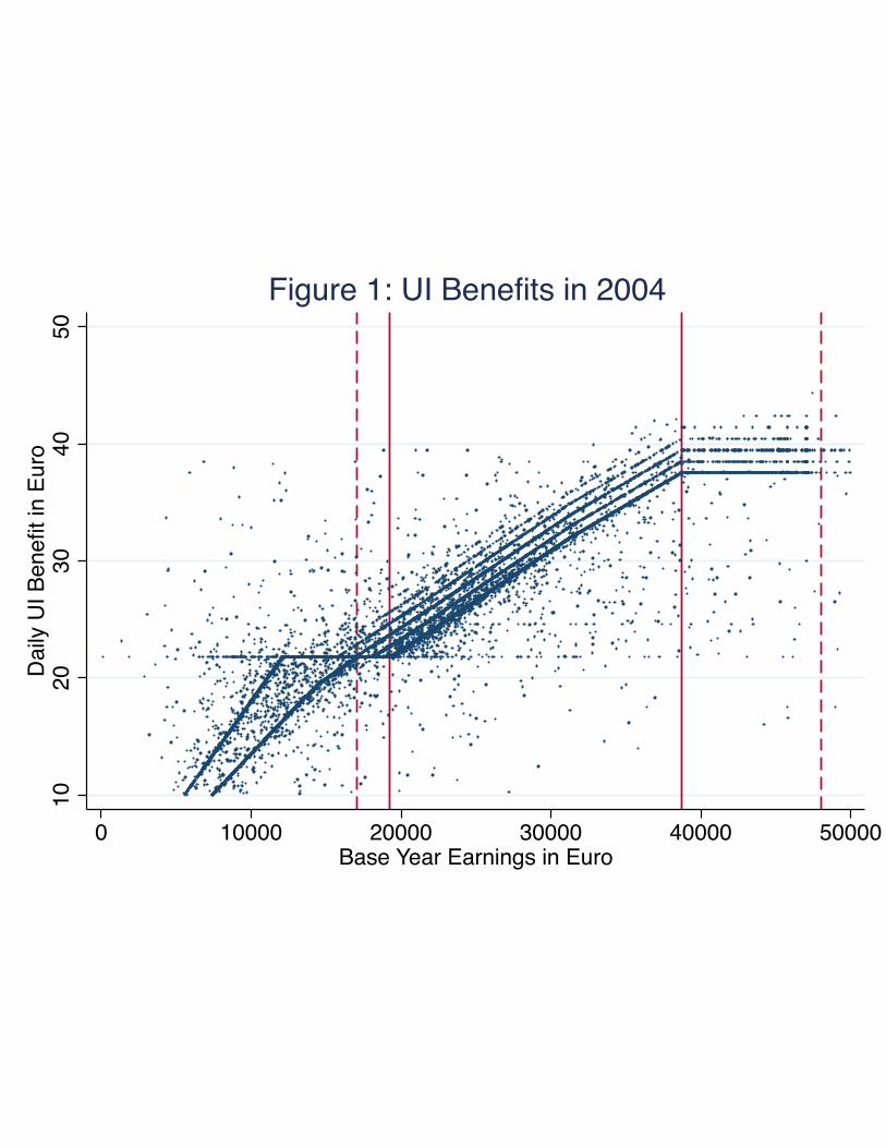
1020
3040
50D
aily
UI B
enefi
t in
Euro
0 10000 20000 30000 40000 50000Base Year Earnings in Euro
Figure 1: UI Benefits in 2004

Figure 2a: Density in Bottom Kink Sample
0.0050
0.0075
0.0100
0.0125
0.0150
0.0175
0.0200
2050 1550 1050 550 50 450 950 1450 1950 2450 2950 3450 3950 4450
Base Year Earnings Relative to T min
Freq
uency
Note: restricted cubic polynomial fit shown.T statistic for continuous slope at kink point = 0.88
Figure 2b: Density in Top Kink Sample
0.000
0.005
0.010
0.015
0.020
0.025
0.030
0.035
0.040
0.045
13950 12450 10950 9450 7950 6450 4950 3450 1950 450 1050 2550 4050 5550
Base Year Earnings Relative to T max
Freq
uency
Note: restricted quartic polynomial fit shown.T statistic for continuous slope at kink point=1.61

2324
2526
2728
Ave
rage
Dai
ly U
I Ben
efit
-2000 -1000 0 1000 2000 3000 4000 5000Base Year Earnings Relative to T-min
Bottom Kink SampleFigure 3: Daily UI Benefits
3035
40A
vera
ge D
aily
UI B
enefi
t
-14000 -9000 -4000 1000 6000Base Year Earnings Relative to T-max
Top Kink SampleFigure 4: Daily UI Benefits

4.4
4.45
4.5
4.55
4.6
Log(
Dur
atio
n)
-2000 -1000 0 1000 2000 3000 4000 5000Base Year Earnings Relative to T-min
Bottom Kink SampleFigure 5: Log Time to Next Job
4.4
4.5
4.6
4.7
Log(
Dur
atio
n)
-14000 -9000 -4000 1000 6000Base Year Earnings Relative to T-max
Top Kink SampleFigure 6: Log Time to Next Job
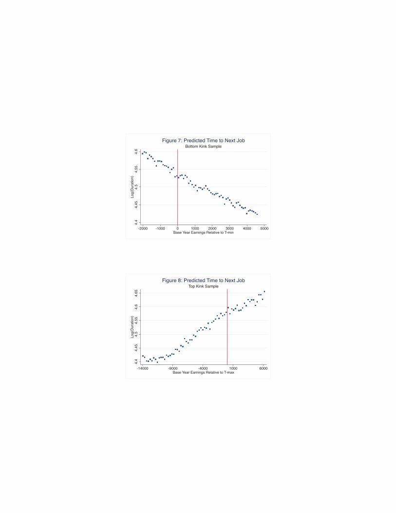
4.4
4.45
4.5
4.55
4.6
Log(
Dur
atio
n)
-2000 -1000 0 1000 2000 3000 4000 5000Base Year Earnings Relative to T-min
Bottom Kink SampleFigure 7: Predicted Time to Next Job
4.4
4.45
4.5
4.55
4.6
4.65
Log(
Dur
atio
n)
-14000 -9000 -4000 1000 6000Base Year Earnings Relative to T-max
Top Kink SampleFigure 8: Predicted Time to Next Job
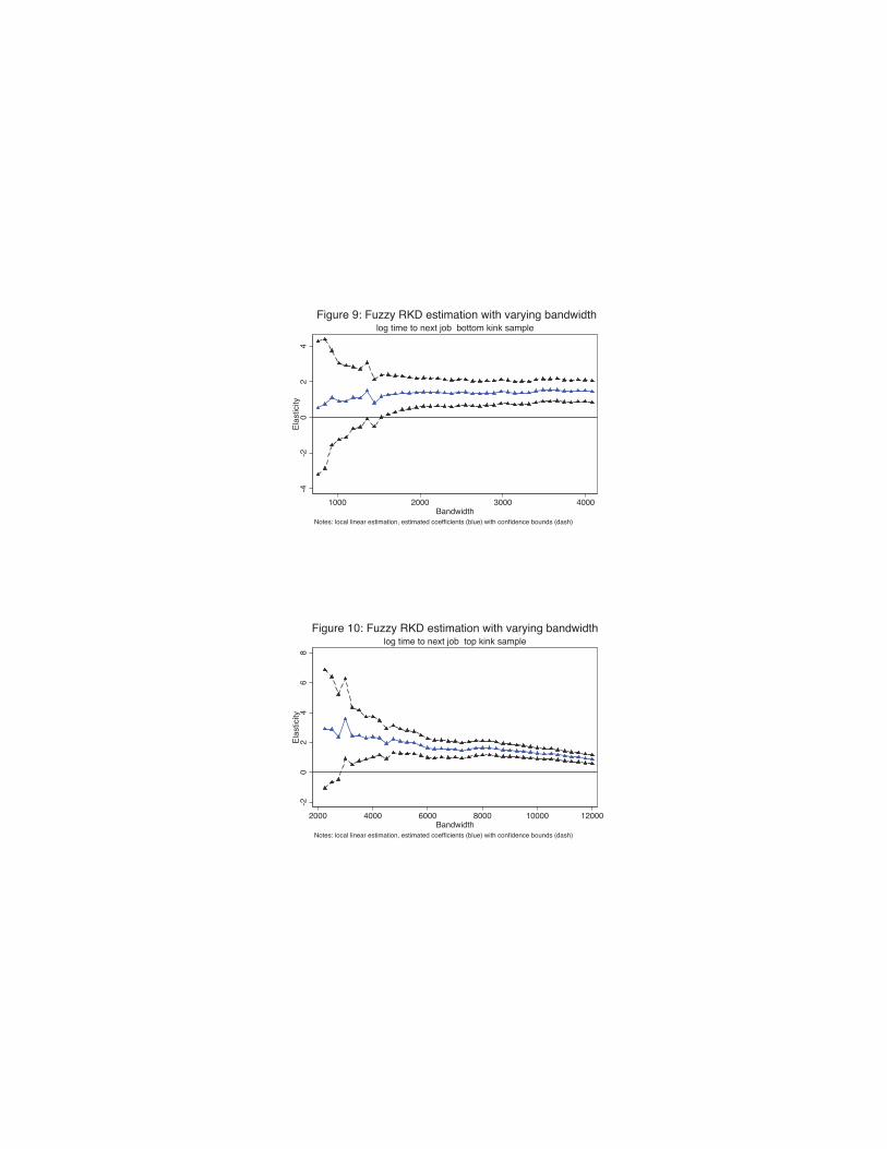
-4-2
02
4E
last
icity
1000 2000 3000 4000Bandwidth
Notes: local linear estimation, estimated coefficients (blue) with confidence bounds (dash)
Figure : Fuzzy RKD estimation with varying bandwidthlog time to next job bottom kink sample
-20
24
68
Ela
stic
ity
2000 4000 6000 8000 10000 12000Bandwidth
Notes: local linear estimation, estimated coefficients (blue) with confidence bounds (dash)
Figure 1 : Fuzzy RKD estimation with varying bandwidthlog time to next job top kink sample

Table 1: Summary Statistics for Bottom and Top Kink Samples of UI Claimants
Mean Std. Dev. Mean Std. Dev.(1) (2) (3) (4)
Baseline earnings (euros) 22,142 2,805 33,847 6,730 Daily UI benefit (euros) 25.2 3.0 33.5 5.7Time to next job (days)* 148.2 129.1 147.4 131.7Duration of initial UI spell (days)** 77.6 67.0 79.8 70.3Total days of UI received 1944.4 1707.0 2679.7 2480.1Fraction exhausted benefits*** 0.09 0.29 0.09 0.29Fraction with time to next job censored 0.19 0.39 0.20 0.40Fraction eligible for extended benefits 0.78 0.41 0.90 0.29Fraction female 0.38 0.48 0.21 0.41Mean Age 33.06 8.48 36.04 7.45Fraction Austrian nationals 0.80 0.40 0.86 0.35Fraction married 0.34 0.47 0.40 0.49Fraction bluecollar occupation 0.65 0.48 0.56 0.50Fraction with higher education 0.11 0.31 0.18 0.38Fraction in Vienna 0.19 0.39 0.21 0.41Tenure in most recent job (Years) 3.39 3.27 4.23 4.20Recalled to last job 0.20 0.40 0.25 0.44Industry: Construction 0.13 0.34 0.23 0.42 Manufacturing 0.20 0.40 0.23 0.42 Trade 0.20 0.40 0.15 0.35 Services 0.26 0.44 0.23 0.42
Number observations
* Time to next job is censored at 365 days.** Claim duration is censored at 39 weeks (maximum entitlement).*** Indicator equals 1 if claim duration = maximum entitlement.
Notes: sample contains UI claimants under the age of 50 with claims in 2001-2012, who had at least 1 year of tenure on their previous job, began their claim within 4 weeks of losing their past job, and had a valid UI claim record and non-missing earnings in the base period prior to the claim. Observations in the bottom kink sample have base period earnings in a range around the bottom kink in the UI benefit schedule; observations in the top kink sample have base period earnings in a range around top kink. See text.
275,293 275,665
Bottom Kink Sample Top Kink Sample

Table 2a: First Stage and Reduced Form Estimated Kinks
Local Linear Local Quad. Local Linear Local Quad.
(1) (2) (3) (4)
A. First Stage Model (Dependent variable = log daily benefit)
Default CCT (with regularization)
Main (Pilot) Bandwidth 448 (929) 813 (1,343) 1,374 (2,760) 1,568 (2,614)
Estimated Kink 1.7 2.1 ‐1.5 ‐1.1
(conventional std error) (1.0) (1.6) (0.7) (2.2)
Estimated Kink ‐ Bias Corrected 1.2 1.2 ‐1.6 ‐2.3
[robust confidence interval] [‐1.6,3.9] [‐2.7,5.1] [‐3.6,0.4] [‐7.6,3.1]
CCT with no regularization
Main (Pilot) Bandwidth 1,257 (1,677) 1,220 (1,646) 2,913 (3,813) 2,128 (3,031)
Estimated Kink 2.3 1.8 ‐1.2 ‐3.6
(conventional std error) (0.2) (0.9) (0.2) (1.4)
Estimated Kink ‐ Bias Corrected 2.1 1.1 ‐0.9 ‐4.7
[robust confidence interval] [1.0,3.1] [‐1.6,3.7] [‐2.0,0.2] [‐8.7,‐0.7]
FG
Main (Pilot) Bandwidth 2,466 (2,380) 2,628 (4,146) 11,603 (6,343) 7,003 (13,081)
Estimated Kink 2.2 2.2 ‐1.9 ‐1.4
(conventional std error) (0.1) (0.3) (0.4) (0.2)
Estimated Kink ‐ Bias Corrected 2.4 1.9 ‐1.4 ‐0.8
[robust confidence interval] [1.7,3.1] [0.4,3.4] [‐2.1,‐0.7] [‐1.9,0.3]
B. Reduced Form Model (Dependent variable = log time to next jobt)
Default CCT (with regularization)
Main (Pilot) Bandwidth 537 (1,062) 598 (986) 1,593 (3,189) 2,546 (4,015)
Estimated Kink 2.2 27.0 2.5 9.2
(conventional std error) (6.7) (23.0) (3.4) (6.7)
Estimated Kink ‐ Bias Corrected 1.3 38.5 3.7 11.0
[robust confidence interval] [‐19.5,22.0] [‐20,97] [‐6.5,13.9] [‐6.9,28.9]
CCT with no regularization
Main (Pilot) Bandwidth 1,330 (1,574) 4,736 (1,971) 2,825 (3,053) 4,225 (4,997)
Estimated Kink 3.1 5.5 ‐3.0 ‐1.4
(conventional std error) (1.7) (2.3) (1.4) (3.1)
Estimated Kink ‐ Bias Corrected 0.9 ‐24.5 ‐1.3 1.4
[robust confidence interval] [‐9.7,11.5] [‐90,41] [‐9.5,7.0] [‐10.8,13.5]
FG
Main (Pilot) Bandwidth 2,501 (3,858) 4,259 (4,918) 4,465 (7,255) 8,001 (12,383)
Estimated Kink 3.0 4.8 ‐3.0 ‐4.1
(conventional std error) (0.8) (2.4) (0.7) (1.5)
Estimated Kink ‐ Bias Corrected 4.2 9.9 ‐5.2 0.0
[robust confidence interval] [‐1.4,9.8] [‐3.6,23.4] [‐8.4,‐1.9] [‐7.0,6.9]
Bottom Kink Top Kink
Notes: Estimated kinks, conventional standard errors and robust confidence intervals are all multiplied by 105. Point estimates and
standard errors are obtained from regressions described in Card et al (2012). Robust CI's and the CCT bandwidths are obtained by a
variant of the Stata package described in Calonico et al (in press).
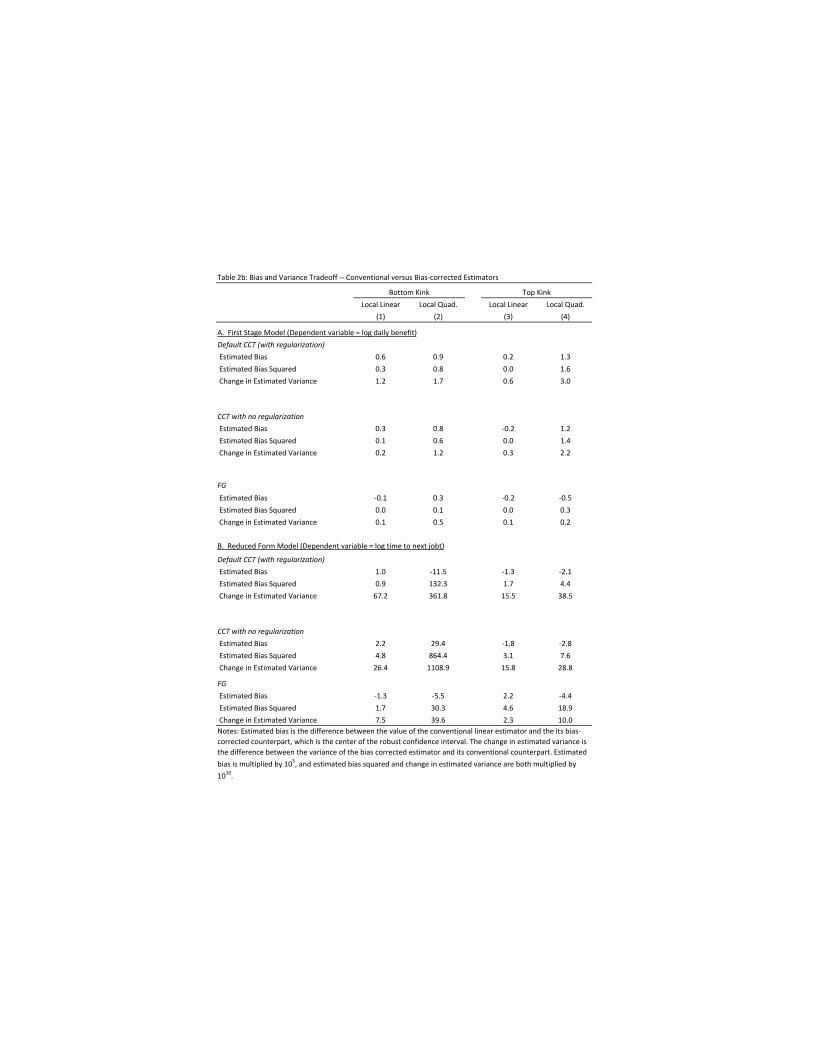
Table 2b: Bias and Variance Tradeoff ‐‐ Conventional versus Bias‐corrected Estimators
Local Linear Local Quad. Local Linear Local Quad.
(1) (2) (3) (4)
A. First Stage Model (Dependent variable = log daily benefit)
Default CCT (with regularization)
Estimated Bias 0.6 0.9 0.2 1.3
Estimated Bias Squared 0.3 0.8 0.0 1.6
Change in Estimated Variance 1.2 1.7 0.6 3.0
CCT with no regularization
Estimated Bias 0.3 0.8 ‐0.2 1.2
Estimated Bias Squared 0.1 0.6 0.0 1.4
Change in Estimated Variance 0.2 1.2 0.3 2.2
FG
Estimated Bias ‐0.1 0.3 ‐0.2 ‐0.5
Estimated Bias Squared 0.0 0.1 0.0 0.3
Change in Estimated Variance 0.1 0.5 0.1 0.2
B. Reduced Form Model (Dependent variable = log time to next jobt)
Default CCT (with regularization)
Estimated Bias 1.0 ‐11.5 ‐1.3 ‐2.1
Estimated Bias Squared 0.9 132.3 1.7 4.4
Change in Estimated Variance 67.2 361.8 15.5 38.5
CCT with no regularization
Estimated Bias 2.2 29.4 ‐1.8 ‐2.8
Estimated Bias Squared 4.8 864.4 3.1 7.6
Change in Estimated Variance 26.4 1108.9 15.8 28.8
FG
Estimated Bias ‐1.3 ‐5.5 2.2 ‐4.4
Estimated Bias Squared 1.7 30.3 4.6 18.9
Change in Estimated Variance 7.5 39.6 2.3 10.0
Bottom Kink Top Kink
Notes: Estimated bias is the difference between the value of the conventional linear estimator and the its bias‐
corrected counterpart, which is the center of the robust confidence interval. The change in estimated variance is
the difference between the variance of the bias corrected estimator and its conventional counterpart. Estimated
bias is multiplied by 105, and estimated bias squared and change in estimated variance are both multiplied by
1010.

FG
Bandwidth
Estimated
Kink
Bias
Corrected
Kink
FG
Bandwidth
Estimated
Kink
Bias
Corrected
Kink
(1) (2) (3) (4) (5) (6)
A. Bottom Kink:
Predicted log time 3,344 0.9 0.8 4,564 1.2 4.0
to next job (0.2) [‐1.0,2.5] (0.8) [‐0.4,8.3]
Female 1,094 0.6 ‐1.1 3,440 ‐0.3 ‐2.1
(1.0) [‐4.0,1.9] (1.2) [‐8.1,4.0]
Age 1,627 29.5 46.8 3,311 32.9 ‐16.5
(9.8) [‐0.4,94] (20.9) [‐122, 89]
Blue collar occup. 2,530 ‐1.5 ‐1.8 4,564 ‐1.5 ‐6.3
(0.3) [‐4.1,0.6] (1.0) [‐12.1,‐0.4]
Recalled to last job 3,199 ‐0.8 0.5 3,194 0.5 ‐2.9
(0.3) [‐1.9,2.9] (1.1) [‐8.1,2.4]
B. Top Kink:
Predicted log time 13,708 0.0 ‐1.5 8,095 ‐1.2 ‐1.9
to next job (0.1) [‐3.0,0.01] (0.5) [‐4.3,0.6]
Female 5,364 ‐0.2 ‐0.9 13,908 ‐1.2 ‐1.5
(0.2) [‐1.9,0.2] (0.4) [‐4,1.1]
Age 6,160 ‐4.6 ‐5.3 9,776 ‐6.1 ‐14.0
(2.6) [‐23.1,12.6] (7.8) [‐55.0,27.0]
Blue collar occup. 2,067 1.5 1.8 5,401 2.6 4.0
(1.0) [‐0.7,4.3] (0.9) [0.7,7.2]
Recalled to last job 5,013 0.6 1.1 13,908 2.7 1.1
(0.2) [‐0.02,2.2] (0.4) [‐1.6,3.7]
Table 3: Estimates of Kinks in Conditional Means of Covariates
Local Quadratic Models
Notes: standard errors in parentheses, robust confidence intervals in square brackets. See notes to
Table 2. All estimates are multiplied by 105. Predicted log time to next job is the estimated
covariate index for this outcome, fit on the pooled bottom and top kink samples. The vector of 59
covariates includes dummies for gender, blue collar occupation, and being recalled to the previous
job, decile of age (9 dummies), decile of previous job tenure (9 dummies), quintile of previous daily
wage (4 dummies), major industry (6 dummies), region (3 dummies), year of claim (7 dummies),
decile of previous firm size (9 dummies), and decile of previous firm's recall rate (9 dummies).
Local Linear Models
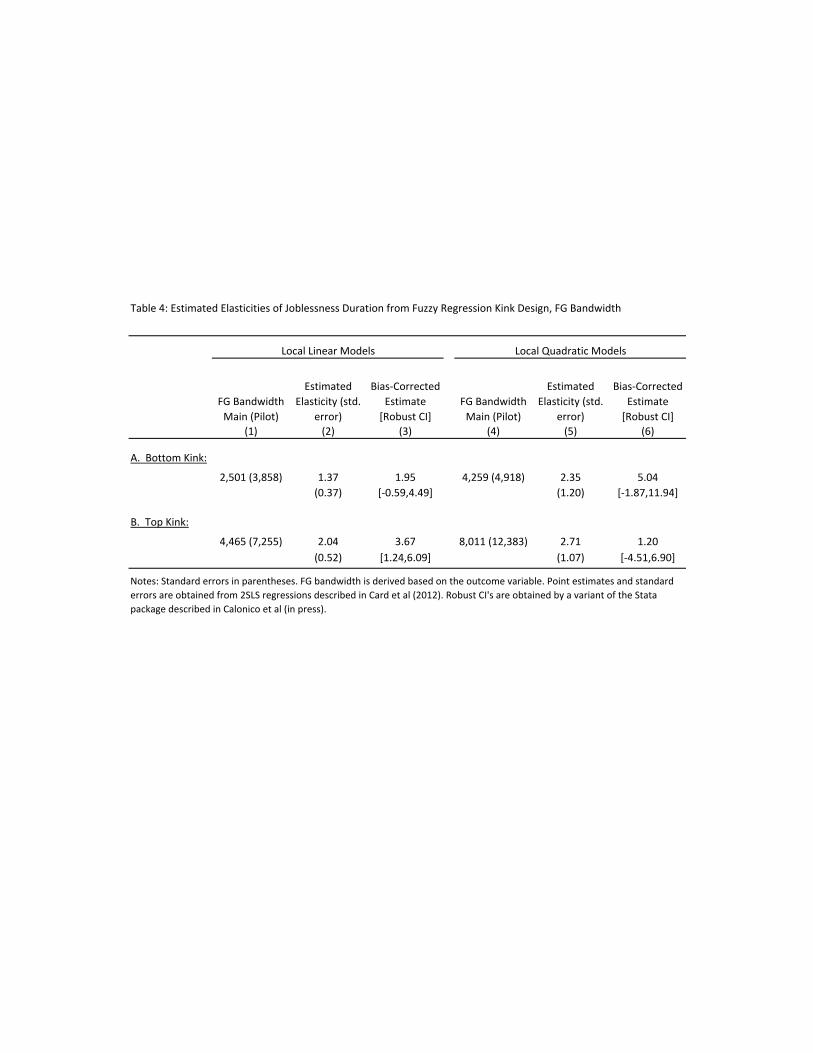
FG Bandwidth
Main (Pilot)
Estimated
Elasticity (std.
error)
Bias‐Corrected
Estimate
[Robust CI]
FG Bandwidth
Main (Pilot)
Estimated
Elasticity (std.
error)
Bias‐Corrected
Estimate
[Robust CI]
(1) (2) (3) (4) (5) (6)
A. Bottom Kink:
2,501 (3,858) 1.37 1.95 4,259 (4,918) 2.35 5.04
(0.37) [‐0.59,4.49] (1.20) [‐1.87,11.94]
B. Top Kink:
4,465 (7,255) 2.04 3.67 8,011 (12,383) 2.71 1.20
(0.52) [1.24,6.09] (1.07) [‐4.51,6.90]
Local Linear Models Local Quadratic Models
Table 4: Estimated Elasticities of Joblessness Duration from Fuzzy Regression Kink Design, FG Bandwidth
Notes: Standard errors in parentheses. FG bandwidth is derived based on the outcome variable. Point estimates and standard
errors are obtained from 2SLS regressions described in Card et al (2012). Robust CI's are obtained by a variant of the Stata
package described in Calonico et al (in press).
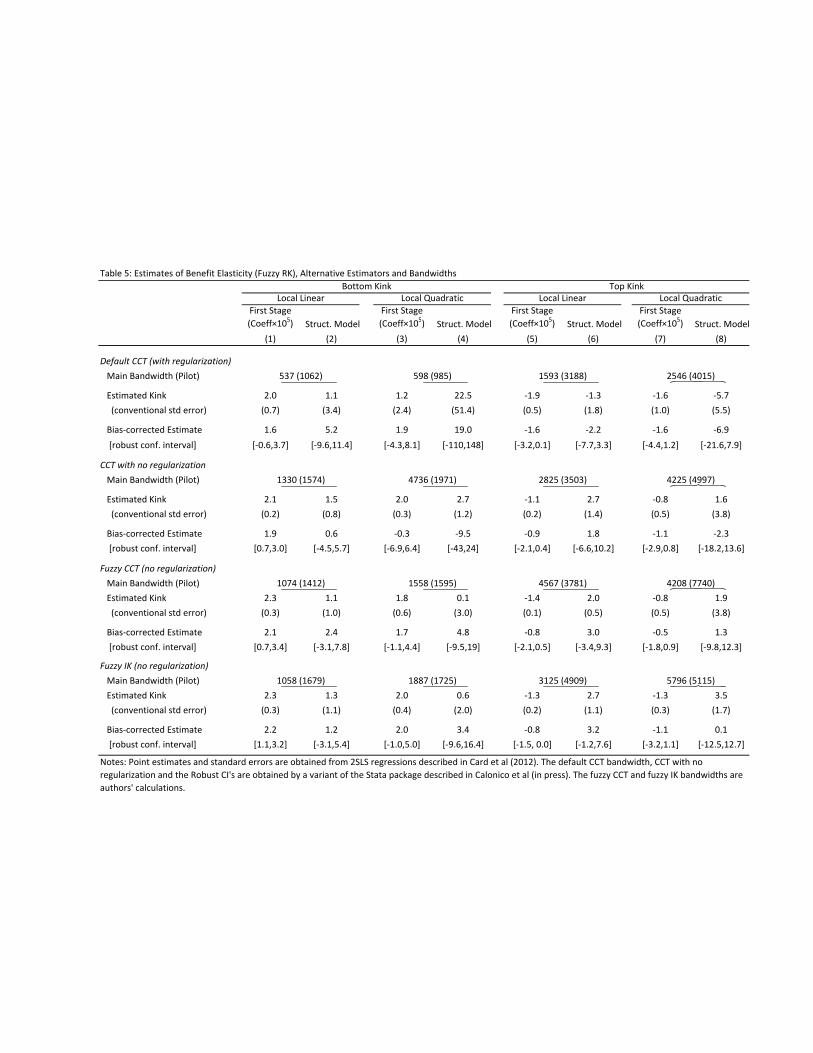
Table 5: Estimates of Benefit Elasticity (Fuzzy RK), Alternative Estimators and Bandwidths
First Stage First Stage First Stage First Stage
(Coeff×105) Struct. Model (Coeff×105) Struct. Model (Coeff×105) Struct. Model (Coeff×105) Struct. Model
(1) (2) (3) (4) (5) (6) (7) (8)
Default CCT (with regularization)
Main Bandwidth (Pilot)
Estimated Kink 2.0 1.1 1.2 22.5 ‐1.9 ‐1.3 ‐1.6 ‐5.7
(conventional std error) (0.7) (3.4) (2.4) (51.4) (0.5) (1.8) (1.0) (5.5)
Bias‐corrected Estimate 1.6 5.2 1.9 19.0 ‐1.6 ‐2.2 ‐1.6 ‐6.9
[robust conf. interval] [‐0.6,3.7] [‐9.6,11.4] [‐4.3,8.1] [‐110,148] [‐3.2,0.1] [‐7.7,3.3] [‐4.4,1.2] [‐21.6,7.9]
CCT with no regularization
Main Bandwidth (Pilot)
Estimated Kink 2.1 1.5 2.0 2.7 ‐1.1 2.7 ‐0.8 1.6
(conventional std error) (0.2) (0.8) (0.3) (1.2) (0.2) (1.4) (0.5) (3.8)
Bias‐corrected Estimate 1.9 0.6 ‐0.3 ‐9.5 ‐0.9 1.8 ‐1.1 ‐2.3
[robust conf. interval] [0.7,3.0] [‐4.5,5.7] [‐6.9,6.4] [‐43,24] [‐2.1,0.4] [‐6.6,10.2] [‐2.9,0.8] [‐18.2,13.6]
Fuzzy CCT (no regularization)
Main Bandwidth (Pilot)
Estimated Kink 2.3 1.1 1.8 0.1 ‐1.4 2.0 ‐0.8 1.9
(conventional std error) (0.3) (1.0) (0.6) (3.0) (0.1) (0.5) (0.5) (3.8)
Bias‐corrected Estimate 2.1 2.4 1.7 4.8 ‐0.8 3.0 ‐0.5 1.3
[robust conf. interval] [0.7,3.4] [‐3.1,7.8] [‐1.1,4.4] [‐9.5,19] [‐2.1,0.5] [‐3.4,9.3] [‐1.8,0.9] [‐9.8,12.3]
Fuzzy IK (no regularization)
Main Bandwidth (Pilot)
Estimated Kink 2.3 1.3 2.0 0.6 ‐1.3 2.7 ‐1.3 3.5
(conventional std error) (0.3) (1.1) (0.4) (2.0) (0.2) (1.1) (0.3) (1.7)
Bias‐corrected Estimate 2.2 1.2 2.0 3.4 ‐0.8 3.2 ‐1.1 0.1
[robust conf. interval] [1.1,3.2] [‐3.1,5.4] [‐1.0,5.0] [‐9.6,16.4] [‐1.5, 0.0] [‐1.2,7.6] [‐3.2,1.1] [‐12.5,12.7]
Notes: Point estimates and standard errors are obtained from 2SLS regressions described in Card et al (2012). The default CCT bandwidth, CCT with no
regularization and the Robust CI's are obtained by a variant of the Stata package described in Calonico et al (in press). The fuzzy CCT and fuzzy IK bandwidths are
authors' calculations.
1074 (1412) 1558 (1595) 4567 (3781) 4208 (7740)
1058 (1679) 1887 (1725) 3125 (4909) 5796 (5115)
537 (1062) 598 (985) 1593 (3188) 2546 (4015)
1330 (1574) 4736 (1971) 2825 (3503) 4225 (4997)
Bottom Kink Top KinkLocal Linear Local Quadratic Local Linear Local Quadratic
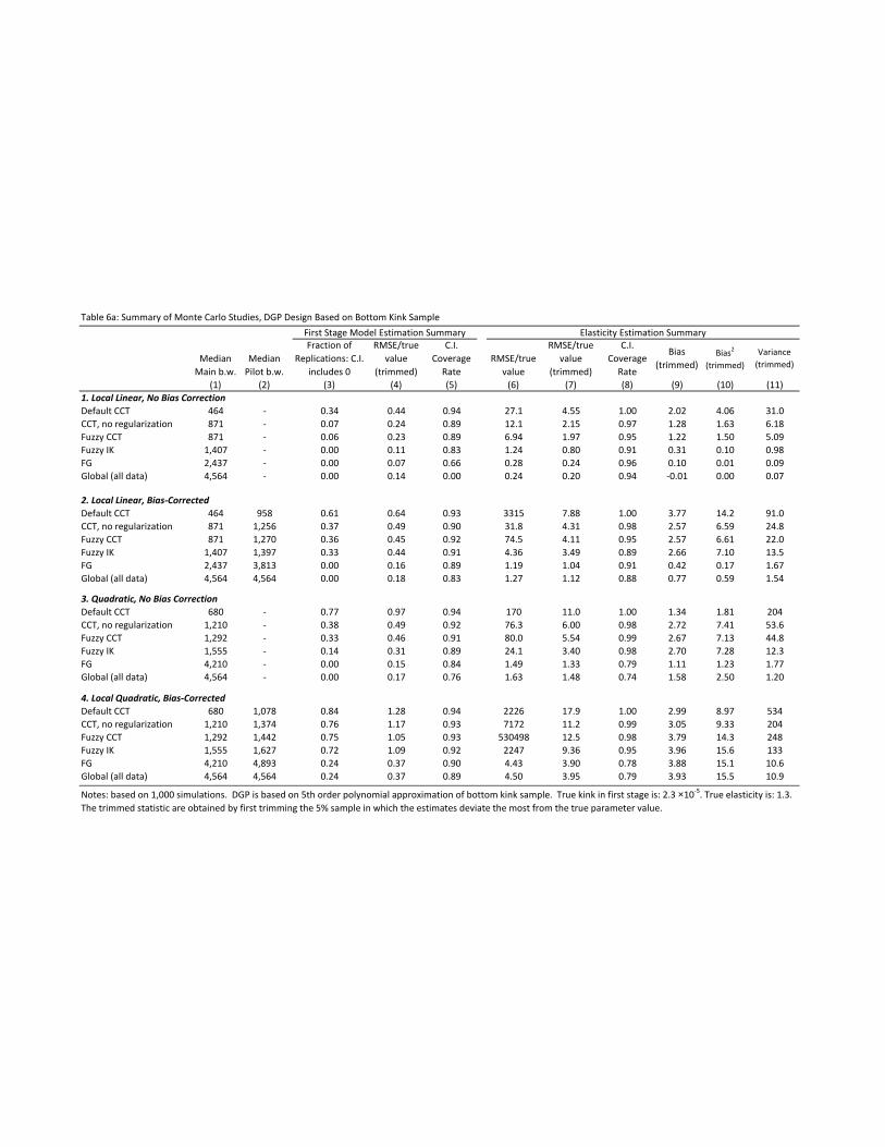
Table 6a: Summary of Monte Carlo Studies, DGP Design Based on Bottom Kink Sample
(1) (2) (3) (4) (5) (6) (7) (8) (9) (10) (11)1. Local Linear, No Bias CorrectionDefault CCT 464 - 0.34 0.44 0.94 27.1 4.55 1.00 2.02 4.06 31.0CCT, no regularization 871 - 0.07 0.24 0.89 12.1 2.15 0.97 1.28 1.63 6.18Fuzzy CCT 871 - 0.06 0.23 0.89 6.94 1.97 0.95 1.22 1.50 5.09Fuzzy IK 1,407 - 0.00 0.11 0.83 1.24 0.80 0.91 0.31 0.10 0.98FG 2,437 - 0.00 0.07 0.66 0.28 0.24 0.96 0.10 0.01 0.09Global (all data) 4,564 - 0.00 0.14 0.00 0.24 0.20 0.94 -0.01 0.00 0.07
2. Local Linear, Bias-CorrectedDefault CCT 464 958 0.61 0.64 0.93 3315 7.88 1.00 3.77 14.2 91.0CCT, no regularization 871 1,256 0.37 0.49 0.90 31.8 4.31 0.98 2.57 6.59 24.8Fuzzy CCT 871 1,270 0.36 0.45 0.92 74.5 4.11 0.95 2.57 6.61 22.0Fuzzy IK 1,407 1,397 0.33 0.44 0.91 4.36 3.49 0.89 2.66 7.10 13.5FG 2,437 3,813 0.00 0.16 0.89 1.19 1.04 0.91 0.42 0.17 1.67Global (all data) 4,564 4,564 0.00 0.18 0.83 1.27 1.12 0.88 0.77 0.59 1.54
3. Quadratic, No Bias CorrectionDefault CCT 680 - 0.77 0.97 0.94 170 11.0 1.00 1.34 1.81 204CCT, no regularization 1,210 - 0.38 0.49 0.92 76.3 6.00 0.98 2.72 7.41 53.6Fuzzy CCT 1,292 - 0.33 0.46 0.91 80.0 5.54 0.99 2.67 7.13 44.8Fuzzy IK 1,555 - 0.14 0.31 0.89 24.1 3.40 0.98 2.70 7.28 12.3FG 4,210 - 0.00 0.15 0.84 1.49 1.33 0.79 1.11 1.23 1.77Global (all data) 4,564 - 0.00 0.17 0.76 1.63 1.48 0.74 1.58 2.50 1.20
4. Local Quadratic, Bias-CorrectedDefault CCT 680 1,078 0.84 1.28 0.94 2226 17.9 1.00 2.99 8.97 534CCT, no regularization 1,210 1,374 0.76 1.17 0.93 7172 11.2 0.99 3.05 9.33 204Fuzzy CCT 1,292 1,442 0.75 1.05 0.93 530498 12.5 0.98 3.79 14.3 248Fuzzy IK 1,555 1,627 0.72 1.09 0.92 2247 9.36 0.95 3.96 15.6 133FG 4,210 4,893 0.24 0.37 0.90 4.43 3.90 0.78 3.88 15.1 10.6Global (all data) 4,564 4,564 0.24 0.37 0.89 4.50 3.95 0.79 3.93 15.5 10.9
Notes: based on 1,000 simulations. DGP is based on 5th order polynomial approximation of bottom kink sample. True kink in first stage is: 2.3 ×10⁻⁵. True elasticity is: 1.3. The trimmed statistic are obtained by first trimming the 5% sample in which the estimates deviate the most from the true parameter value.
RMSE/true value
RMSE/true value
(trimmed)
C.I. Coverage
Rate
Elasticity Estimation Summary
Bias (trimmed)
Bias2
(trimmed)Variance
(trimmed)Median Main b.w.
Median Pilot b.w.
First Stage Model Estimation SummaryFraction of
Replications: C.I. includes 0
RMSE/true value
(trimmed)
C.I. Coverage
Rate

Table 6b: Summary of Monte Carlo Studies, DGP Design Based on Top Kink Sample
(1) (2) (3) (4) (5) (6) (7) (8) (9) (10) (11)1. Local Linear, No Bias CorrectionDefault CCT 1,371 - 0.62 0.59 0.81 78.8 3.66 0.99 0.50 0.25 53.5CCT, no regularization 2,683 - 0.15 0.34 0.72 7.37 1.25 0.91 -0.02 0.00 6.30Fuzzy CCT 2,301 - 0.25 0.43 0.72 81.0 1.97 0.94 0.04 0.00 15.5Fuzzy IK 3,254 - 0.00 0.20 0.74 0.76 0.52 0.94 0.39 0.15 0.94FG 4,465 - 0.00 0.15 0.77 0.48 0.36 0.82 0.11 0.01 0.52Global (all data) 13,908 - 0.00 0.55 0.00 0.81 0.80 0.00 -1.60 2.56 0.01
2. Local Linear, Bias-CorrectedDefault CCT 1,371 2,842 0.88 0.90 0.79 12323 10.1 0.99 2.32 5.40 400CCT, no regularization 2,683 3,673 0.68 0.76 0.69 473 3.12 0.93 0.01 0.00 39.1Fuzzy CCT 2,301 3,570 0.68 0.79 0.69 18102 5.12 0.95 0.61 0.38 104Fuzzy IK 3,254 4,604 0.44 0.59 0.64 2.36 1.67 0.90 0.77 0.59 10.5FG 4,465 7,300 0.00 0.19 0.88 1.17 0.95 0.81 1.50 2.26 1.36Global (all data) 13,908 13,908 0.00 0.22 0.72 0.92 0.87 0.44 1.57 2.45 0.55
3. Quadratic, No Bias CorrectionDefault CCT 2,033 - 0.90 1.10 0.89 93.6 7.95 1.00 -2.04 4.18 249CCT, no regularization 3,459 - 0.66 0.77 0.72 52.6 6.70 0.96 -0.39 0.15 180Fuzzy CCT 3,613 - 0.64 0.72 0.69 97.2 6.00 0.97 -0.59 0.35 144Fuzzy IK 4,964 - 0.34 0.49 0.71 43.4 3.03 0.92 0.26 0.07 36.7FG 8,060 - 0.00 0.15 0.91 1.06 0.93 0.84 1.59 2.53 0.94Global (all data) 13,908 - 0.00 0.20 0.58 2.07 1.97 0.03 3.79 14.3 1.16
4. Local Quadratic, Bias-CorrectedDefault CCT 2,033 3,232 0.91 1.40 0.90 1013 15.0 1.00 -1.40 1.96 904CCT, no regularization 3,459 4,088 0.91 1.42 0.78 21785 26.5 0.99 1.25 1.55 2803Fuzzy CCT 3,613 4,264 0.92 2.17 0.79 16114 25.9 0.98 3.77 14.2 2677Fuzzy IK 4,964 5,033 0.93 1.44 0.68 65325 14.3 0.93 1.03 1.05 821FG 8,060 12,471 0.71 0.63 0.62 1.89 1.53 0.93 0.36 0.13 9.2Global (all data) 13,908 13,908 0.79 0.71 0.49 2.36 1.89 0.93 0.94 0.88 13.5
Bias2
(trimmed)Variance
(trimmed)
Notes: based on 1,000 simulations. DGP is based on 5th order polynomial approximation of top kink sample. True kink in first stage is: -1.4 × 10⁻⁵ . True elasticity is: 2.0. The trimmed statistic are obtained by first trimming the 5% sample in which the estimates deviate the most from the true parameter value.
Elasticity Estimation SummaryRMSE/true
value (trimmed)
C.I. Coverage
Rate
First Stage Model Estimation Summary
Median Main b.w.
Median Pilot b.w.
Fraction of Replications: C.I.
includes 0
RMSE/true value
(trimmed)
C.I. Coverage
RateRMSE/true
value
Bias (trimmed)

Supplemental Appendix
A Identification
A.1 Proofs of Proposition 1 and 2
In order to prove Proposition 1, we first present and prove the following Lemmas.
Lemma 1. Let ϕ(x, t) : I× [c,d]→ R where I is a compact subset of Rm. Suppose ϕ(x, t) and its partial
derivative, ϕ2(x, t), are continuous and that ϕ is integrable with respect to the probability measure α for
each t. Then f (t) =∫
ϕ(x, t)dα(x) is continuously differentiable on [c,d].
Proof: By Theorem 5 (p.97) of Roussas (2004), f ′(t) =∫
ϕ2(x, t)dα(x) for all t ∈ [c,d]. Let s1,s2 ∈ [c,d]
| f ′(s1)− f ′(s2)| = |∫
ϕ2(x,s1)dα(x)−∫
ϕ2(x,s2)dα(x)|
6∫|ϕ2(x,s1)−ϕ2(x,s2)|dα(x)
The continuity of ϕ2(x, t) on the compact set I× [c,d] implies uniform continuity, and therefore we can
choose a δ such that |s1− s2| < δ | implies |ϕ2(x,s1)−ϕ2(x,s2)| < ε
α(I) for all x ∈ I, which in turn implies
that | f ′(s1)− f ′(s2)|< ε . QED
Lemma 2. Under Assumptions 1(i), 3(ii) and 4, f (v) is continuously differentiable and strictly positive on
IV .
Proof: The continuous differentiability of f (v) follows from Assumption 1(i), Assumption 4 and Lemma
1. f (V )>∫
AUfV |U=u(v)dFU(u)> 0 follows directly from Assumption 3(ii).
In order to prove Proposition 2, we present and prove the following lemmas. Let S be a sub-vector of
the random vector (U,ε,UB′ ,UV ′) that at least includes U and ε , and let S∗denote the vector of the random
variables in (U,ε,UB′ ,UV ′) but not in S. Let Q be a sub-vector of the random vector (ε,UB′ ,UV ′) that at least
includes ε , and let Q∗denote the vector of the random variables in (U,ε,UB′ ,UV ′) but not in Q. Let IV ∗ , IS,
IS∗ , IQ and IQ∗ be the smallest closed rectangle that contains the support of V ∗, S, S∗,Q and Q∗, respectively.
In the proofs, we only consider the case where π i j(V,U,ε,UV ′ ,UB′)> 0 for all i, j = 0,1 since the proofs for
the cases where some of the π i j = 0 are similar in spirit and simpler. Also, we abstract away in the following

lemmas from the potential issues in situations where the conditioning set, e.g. S = s, is of measure 0 (cf
Borel-Kolmogorov paradox) because the integrals in Proposition is 2 are over the distribution of S.
Lemma 3. a) fS∗|S=s (s∗) is continuous on IS∗,S; b) fQ∗|Q=q(q∗) is continuous on IQ∗,Q.
Proof: We prove part a), and the proof for part b) is similar. There are three cases 1) S∗ = UV ′ , 2)
S∗ =UB′ and 3) S∗ = (UV ′ ,UB′). For case 1),
fUV ′ |UB′=uB′ ,U=u,ε=e(uV ′) =fUV ′ ,UB′ |U=u,ε=e(uV ′ ,uB′)
fUB′ |U=u,ε=e(uB′)(10)
=
∫fV,UV ′ ,UB′ |U=u,ε=e(v,uV ′ ,uB′)dv∫ ∫
fV,UV ′ ,UB′ |U=u,ε=e(v,uV ′ ,uB′)dvduV ′
Note that the numerator of (10) is exactly fS∗|S=s (s∗) in case 3). Both the numerator and the denominator
are continuous as guaranteed by Assumption 4a and Proposition 1 in 17.5 of Zorich (2004). Since the
denominator is strictly positive, fUV ′ |UB′=uB′ ,U=u,ε=e(uV ′) is continuous. The proof for case 2) is analogous
with the roles of UV ′ and UB′ exchanged.
Lemma 4. a) ∂
∂v fV |S=s (v) is continuous on IV,S. b) ∂
∂v fV |Q=q (v) is continuous on IV,Q.
Proof: We only prove part a), and the proof of part b) is similar. Note that
fV |S=s,S∗=s∗(v) =fV,UV ′ ,UB′ |U=u,ε=e(v,uV ′ ,uB′)
fUV ′ ,UB′ |U=u,ε=e(uV ′ ,uB′)
fV |S=s(v) =∫ fV,UV ′ ,UB′ |U=u,ε=e(v,uV ′ ,uB′)
fUV ′ ,UB′ |U=u,ε=e(uV ′ ,uB′)fS∗|S=s (s
∗)ds∗
where the first line follows by Bayes’ rule, and we integrate both sides over fS∗|S=s (s∗) to arrive at the
second line. Taking derivatives with respect to v on both sides, interchanging differentiation and integration
(permitted by Assumption 4a, Lemma 3 and Roussas (2004)), we obtain the result following Lemma 1.
Lemma 5. a) ∂
∂v∗ fV ∗|S=s(v∗) is continuous on IV ∗,S. b) ∂
∂v∗ fV ∗|Q=q(v∗) is continuous on IV ∗,Q.
Proof: We only prove part a), and the proof of part b) is similar. Note that after applying Bayes’ Rule

and re-arranging, we obtain
fV ∗ |S=s,S∗=s∗ (v∗) = Pr [UV = 0|S = s,S∗ = s∗] fV |S=s,S∗=s∗ ,UV =0 (v
∗)
+Pr [UV 6= 0|S = s,S∗ = s∗] fV ∗ |S=s,S∗=s∗ ,UV 6=0 (v∗)
= Pr [UV = 0|S = s,S∗ = s∗]Pr [UV = 0|V = v∗,S = s,S∗ = s∗]fV |S=s,S∗=s∗ (v∗)
Pr [UV = 0|S = s,S∗ = s∗]
+Pr [UV 6= 0|S = s,S∗ = s∗]Pr [UV 6= 0|V = v∗−uV ′ ,S = s,S∗ = s∗]fV |S=s,S∗=s∗ (v∗−uV ′ )
Pr [UV 6= 0|S = s,S∗ = s∗]
= Pr [UV = 0|V = v∗,S = s,S∗ = s∗] fV |S=s,S∗=s∗ (v∗)
+Pr [UV 6= 0|V = v∗−uV ′ ,S = s,S∗ = s∗] fV |S=s,S∗=s∗ (v∗−uV ′ )
Multiplying both sides of the last line by fS∗|S=s (s∗) and integrating over s∗, taking the partial derivative
with respect to v∗, and applying Assumptions 4a and 5 and Lemmas 3 and 4, we have the desired result.
Lemma 6. a) ∂
∂v∗ Pr[GV = i,GB = j|V ∗ = v∗,S = s] and ∂
∂v∗ Pr[GV = i|V ∗ = v∗,S = s] are continuous on
the set (v∗,s) : fV ∗|S=s(v∗) > 0 for i, j = 0,1. b) ∂
∂v∗ Pr[GV = i,GB = j|V ∗ = v∗,Q = q] and ∂
∂v∗ Pr[GV =
i|V ∗ = v∗,Q = q] are continuous on the set (v∗,q) : fV ∗|Q=q(v∗)> 0 for i, j = 0,1.
Proof: Again we only prove part a). First, note that the continuous differentiability of Pr[GV = i,GB =
j|V ∗ = v∗,S = s] and Pr[GV = i|V ∗ = v∗,S = s] is only needed on the set (v∗,s) : fV ∗|S=s(v∗) > 0 for the
purpose of proving Proposition 2 because these quantities are always multiplied by fV ∗|S=s(v∗) when they
appear in subsequent proofs. We consider the two cases of i = 0,1 separately. For case 1 where i = 0,
Pr [GV = 0,GB = j|V ∗ = v∗,S = s] = fV ∗ |S=s,GV =0,GB= j (v∗)
Pr [GV = 0,GB = j|S = s]fV ∗ |S=s (v∗)
= fV |S=s,GV =0,GB= j (v∗)
Pr [GV = 0,GB = j|S = s]fV ∗ |S=s (v∗)
= fV |S=s,GV =0,GB= j (v∗)
Pr [GV = 0,GB = j|S = s]fV |S=s (v∗)
fV |S=s (v∗)fV ∗ |S=s (v∗)
= Pr [GV = 0,GB = j|V = v∗,S = s]fV |S=s (v∗)fV ∗ |S=s (v∗)
=∫
π0 j (v∗,u,ε,uV ′ ,uB′ ) fS∗ |V=v∗,S=s (s
∗)ds∗fV |S=s (v∗)fV ∗ |S=s (v∗)
=∫
π0 j (v∗,u,ε,uV ′ ,uB′
)fV |S∗=s∗ ,S=s (v
∗)fS∗|S=s (s∗)fV |S=s (v∗)
ds∗fV |S=s (v∗)fV ∗ |S=s (v∗)
.
The partial derivative of the right hand side w.r.t. v∗ in the last line is continuous on IV ∗,S by Assumption 5
and Lemmas 3, 4 and 5. For case 2 where i = 1,

Pr[GV = 1,GB = j|V ∗ = v∗,S = s]
=∫
Pr[GV = 1,GB = j|V ∗ = v∗,S = s,S∗ = s∗] fS∗ |V ∗=v∗ ,S=s(s∗)ds∗
=∫
Pr[GV = 1,GB = j|V = v∗−uV ′ ,S = s,S∗ = s∗]fV ∗ |S=s,S∗=s∗ (v∗) fS∗ |S=s(s∗)
fV ∗ |S=s(v∗)ds∗
=∫
π1 j(v∗−uV ′ ,u,ε,uV ′ ,uB′ )
fV ∗ |S=s,S∗=s∗ (v∗) fS∗ |S=s(s∗)fV ∗ |S=s(v∗)
ds∗.
Its partial derivative w.r.t. v∗ is continuous on IV ∗,S for the same reason as in case 1.Since Pr[GV = i|V ∗ = v∗,S = s] = ∑ j Pr[GV = i,GB = j|V ∗ = v∗,S = s], the continuous differentiability with respect to v∗
of Pr[GV = i,GB = j|V ∗ = v∗,S = s] implies that of Pr[GV = i|V ∗ = v∗,S = s].
Proof of Proposition 2
For part (a), the proof is the same as for part (a) in Proposition 1, replacing V with V ∗, letting the pair
(U,ε) serve the role of U and using Lemma 5.For part (b), we can write
E [Y |V ∗ = v∗] =∫
E [Y |V ∗ = v∗,U = u,ε = e]dFU,ε|V ∗=v∗ (u,e)
=∫
(E [Y |UV = 0,V ∗ = v∗,U = u,ε = e]Pr [UV = 0|V ∗ = v∗,U = u,ε = e]+
E [Y |UV 6= 0,V ∗ = v∗,U = u,ε = e]Pr [UV 6= 0|V ∗ = v∗,U = u,ε = e])dFU,ε|V ∗=v∗ (u,e)
=∫ (
z1z2 +
[∫z3z4duV ′
]· [1− z2]
)z5dFU,ε (u,e). (11)
where the second line follows from the law of iterated expectations, and to ease exposition below, we use
the notation:
z1 ≡ y(b(v∗,e) ,v∗,u)
z2 ≡ Pr [V =V ∗|V ∗ = v∗,U = u,ε = e]
z3 ≡ y(b(v∗−uV ′ ,e) ,v∗−uV ′ ,u)
z4 ≡ fUV ′ |UV 6=0,V ∗=v∗,U=u,ε=e (uV ′)
z5 ≡fV ∗|U=u,ε=e(v∗)
fV ∗(v∗).
The derivative of E [Y |V ∗ = v∗] in equation (11) with respect to v∗ is
dE [Y |V ∗ = v∗]dv∗
=∫
z′1z2z5dFU,ε (u,e)+∫
z1∂ (z2z5)
∂v∗dFU,ε (u,e)
+∫
∂ [(∫
z3z4duV ′) [1− z2]z5]
∂v∗dFU,ε (u,e) (12)
where z′j denotes the partial derivative of z j with respect to v∗, provided that the integrands are continuous.

In a parallel fashion, we can write
E[B∗|V ∗ = v∗] =∫[z6 + z8(1− z7)]z13
+[(∫
z9z10duV ′ )z11 +(∫(z9 +uB′ )z12duV ′duB′ )(1− z11)](1− z13)z14dFε (e)
with
z6 ≡ b(v∗,e)
z7 ≡ Pr[UB = 0|UV = 0,V ∗ = v∗,ε = e]
z8 ≡∫
uB′ fUB′ |UV=0,UB 6=0,V ∗=v∗,ε=e(uB′)duB′
z9 ≡ b(v∗−uV ′ ,e)
z10 ≡ fUV ′ |UB=0,UV 6=0,V ∗=v∗,ε=e(uV ′)
z11 ≡ Pr[UB = 0|UV 6= 0,V ∗ = v∗,ε = e]
z12 ≡ fUV ′ ,UB′ |UV 6=0,UB 6=0,V ∗=v∗,ε=e(uV ′ ,uB′)
z13 ≡ Pr[V =V ∗|V ∗ = v∗,ε = e]
z14 ≡fV ∗|ε=e(v∗)
fV ∗(v∗).
And the analogous derivative with respect to v∗ is
dE [B∗|V ∗ = v∗]dv∗
=∫
z′6z13z14dFε (e)+∫
z6∂
∂v∗(z13z14)dFε (e)
+∂
∂v∗
∫[z8(1− z7)z13z14]dFε (e)
+∂
∂v∗
∫∫
z9z10duV ′ · z11 +∫ ∫(z9 +uB′)z12duV ′duB′ · (1− z11)(1− z13z14)dFε (e), (13)
provided that the integrands are continuous.
The proof of part (b) follows from showing that the partial derivatives of z2,∫
z3z4duV ′ , z5, z7, z8,∫z9z10duV ′ , ,z11,
∫ ∫(z9 + uB′)z12duV ′duB′ and z13z14, with respect to v∗ are continuous, and noting that z1
and z6 are continuous by Assumptions 1a, 2, and 3a. From this it follows that there is no discontinuity in all
but the first term on the right hand side of (12) and (13) at v∗ = 0 and that the RKD estimand is the ratio of
the discontinuities in the first terms of those two equations.
As shown by Lemma 6, z2 is continuously differentiable in v∗.

z4 is continuously differentiable in v∗ because
fUV ′ |UV 6=0,V ∗=v∗ ,U=u,ε=e (uV ′ ) =Pr [UV 6= 0|UV ′ = uV ′ ,V ∗ = v∗,U = u,ε = e] fUV ′ |V ∗=v∗ ,U=u,ε=e (uV ′ )
Pr [UV 6= 0|V ∗ = v∗,U = u,ε = e]
=(1−Pr [UV = 0|UV ′ = uV ′ ,V ∗ = v∗,U = u,ε = e])
fV∗|UV ′=uV ′ ,U=u,ε=e(v∗) fUV ′ |U=u,ε=e(uV ′ )
fV∗|U=u,ε=e(v∗)
1− z2,
and the derivative of the last line is continuous by Lemmas 3, 5 and 6.
We break up the integral∫
z3z4duV ′ into two pieces
∫z3z4duV ′ =
∫ v∗
cUV ′
z3z4duV ′ +∫ dUV ′
v∗z3z4duV ′
=∫ v∗
cUV ′
y(b+ (v∗−uV ′ ,e) ,v
∗−uV ′ ,u)
z4duV ′
+∫ dUV ′
v∗y(b− (v∗−uV ′ ,e) ,v
∗−uV ′ ,u)
z4duV ′
where cUV ′ and dUV ′ are the lower and upper end point of the support of UV ′ , b+(v,e) = b(v,e) for v > 0 and
all e and b−(v,e) = b(v,e) for v 6 0 and all e. Denote y(b± (v∗−uV ′ ,e) ,v∗−uV ′ ,u) by z±3 . Note that z+3and z−3 are continuously differentiable in v∗ on [cUV ′ ,v
∗] and [v∗,dUV ′ ] respectively by Assumptions 1a, 2 and
3a, where cUV ′ and dUV ′ are the lower and upper endpoints of the support IU ′V . Since z4 is also continuously
differentiable as shown above, we can apply the Newton-Leibniz formula, which yields
∂
∂v∗(∫ v∗
cUV ′
z+3 z4duV ′ +∫ dUV ′
v∗z−3 z4duV ′) =
∫ v∗
cUV ′
∂
∂v∗(z+3 z4)duV ′ +
∫ dUV ′
v∗
∂
∂v∗(z−3 z4)duV ′
+z+3 z4|uV ′=v∗ − z−3 z4|uV ′=v∗ .
By Assumptions 1a and 3a, z3 is continuous, and it follows that z+3 z4|uV ′=v∗ − z−3 z4|uV ′=v∗ = 0. Since∫ v∗cUV ′
∂
∂v∗ (z+3 z4)duV ′ and
∫ dUV ′v∗
∂
∂v∗ (z−3 z4)duV ′ are continuous,
∫z3z4duV ′ is continuously differentiable in v∗.
z5 is continuously differentiable in v∗ by Lemma 5 and Assumption 3a–note that the continuous differ-
entiability of fV ∗(v∗) =∫
fV ∗|U=u,ε=edFU,ε(u,e) is a part of Corollary 1, and it follows directly from Lemma
5; z6 is continuously differentiable by Assumption 3a, and z7 is continuously differentiable in v∗ because
Pr[UB = 0|UV = 0,V ∗ = v∗,ε = e] =Pr[UV = 0,UB = 0|V ∗ = v∗,ε = e]
Pr[UV = 0|V = v∗,ε = e]
where the derivative of the right hand side is continuous in v∗ by Lemma 6.

z8 is continuously differentiable in v∗ because
∫uB′ fUB′ |UV =0,UB 6=0,V ∗=v∗ ,ε=e(uB′ )duB′
=∫
uB′ Pr[UV = 0|UB′ = uB′ ,V∗ = v∗,ε = e]
fUB′ |V ∗=v∗ ,ε=e(uB′ )
Pr[UV = 0|V ∗ = v∗,ε = e]duB′
=∫
uB′ Pr[UV = 0|UB′ = uB′ ,V∗ = v∗,ε = e]
fV ∗ |UB′=uB′ ,ε=e(v∗) fUB′ |ε=e(uB′ )
fV ∗ |ε=e(v∗)Pr[UV = 0|V = v∗,ε = e]duB′
where the continuous differentiability of the last line in v∗ is implied by Lemmas 3, 5 and 6. By a similar
application of the Bayes’ Rule, we can show that z10 is continuously differentiable in v∗. Consequently,∫z9z10duV ′ is continuously differentiable in v∗ by applying the same argument used for
∫z3z4duV ′ .
The quantity z11 is continuously differentiable in v∗ because of Lemma 6 and that
z11 =Pr[UB = 0,UV 6= 0|V ∗ = v∗,ε = e]
Pr[UV 6= 0|V ∗ = v∗,ε = e]
z12 can be expressed as
fUV ′ ,UB′ |UV 6=0,UB 6=0,V ∗=v∗ ,ε=e(uV ′ ,uB′ )
=Pr[UV 6= 0,UB 6= 0|UV ′ = uV ′ ,UB′ = uB′ ,V ∗ = v∗,ε = e]
Pr[UV 6= 0,UB 6= 0|V ∗ = v∗,ε = e]fUV ′ ,UB′ |V ∗=v∗ ,ε=e(uV ′ ,uB′ )
=Pr[UV 6= 0,UB 6= 0|UV ′ = uV ′ ,UB′ = uB′ ,V ∗ = v∗,ε = e]
Pr[UV 6= 0,UB 6= 0|V ∗ = v∗,ε = e]·
fV ∗ |UV ′=uV ′ ,UB′=uB′ ,ε=e(v∗)
fV ∗|ε=e(v∗)fUV ′ ,UB′ |ε=e(uV ′ ,uB′ ),
and z12 is continuously differentiable by Lemmas 3, 5 and 6. It follows that∫ ∫
(z9 + uB′)z12duV ′duB′ is
continuously differentiable by the same argument as that for∫
z3z4duV ′ .Finally, z13 is continuously differen-
tiable in v∗ by Lemma 6 and z14 by Lemma 5 and Assumption 3a.
As a result of the smoothness of the above terms and Theorem 5 on p. 97 of Roussas (2004), we can
write
limv0→0+
dE[Y |V ∗ = v∗]dv∗
∣∣∣∣v∗=v0
− limv0→0−
dE[Y |V ∗ = v∗]dv∗
∣∣∣∣v∗=v0
= limv0→0+
∫z′1z2z5dFU,ε (u,e)− lim
v0→0−
∫z′1z2z5dFU,ε (u,e)
=∫ (
limv0→0+
z′1− limv0→0−
z′1
)z2z5|v∗=v0
dFU,ε (u,e)
=∫
y1 (b(0,e) ,0,u)(b+1 (e)−b−1 (e)
)z2z5|v∗=v0
dFU,ε (u,e). (14)
The interchange of limit of integration is allowed by the dominated convergence theorem since z′1z2z5 is

continuous over a compact rectangle. The last line follows from Assumptions 1a and 3a.
Similarly, we can write
limv0→0+
dE [B∗|V ∗ = v∗]dv∗
∣∣∣∣v∗=v0
− limv0→0−
dE [B∗|V ∗ = v∗]dv∗
∣∣∣∣v∗=v0
= limv0→0+
∫z′6z13z14dFε (e)− lim
v0→0−
∫z′6z13z14dFε (e)
=∫ (
limv0→0+
z′6− limv0→0−
z′6
)z13z14|v∗=v0
dFε (e)
=∫ (
b+1 (e)−b−1 (e))
z13z14|v∗=v0dFε (e). (15)
Finally, consider the term z2z5|v∗=v0. First, a similar argument as in 6 leads to
z2 = Pr [V =V ∗|V = v∗,U = u,ε = e]fV |U=u,ε=e (v∗)
fV ∗|U=u,ε=e (v∗).
After applying Bayes’ Rule and re-arranging, we have
z2z5|v∗=v0= Pr [V =V ∗|V = 0,U = u,ε = e]
fV |U=u,ε=e (0)fV ∗|U=u,ε=e (0)
fV ∗|U=u,ε=e(0)fV ∗(0)
= Pr [V =V ∗|V = 0,U = u,ε = e]fV |U=u,ε=e (0)
fV (0)fV (0)fV ∗ (0)
.
Similarly, we can derive
z13z14|v∗=v0= Pr [V =V ∗|V = 0,ε = e]
fV |ε=e (0)fV (0)
fV (0)fV ∗ (0)
.
Because fV (0)fV∗ (0)
can be pulled out of the integral in both (14) and (15), we have the result
limv0→0+
dE[Y |V ∗=v∗]dv∗
∣∣∣v∗=v0
− limv0→0−
dE[Y |V ∗=v∗]dv∗
∣∣∣v∗=v0
limv0→0+
dE[B∗|V ∗=v∗]dv∗
∣∣∣v∗=v0
− limv0→0−
dE[B∗|V ∗=v∗]dv∗
∣∣∣v∗=v0
=∫
y1 (b(0,e) ,0,u)ϕ (u,e)dFU,ε (u,e)
where ϕ (u,e) =Pr[UV=0|V=0,U=u,ε=e](b+1 (e)−b−1 (e))
fV |U=u,ε=e(0)
fV (0)∫Pr[UV=0|V=0,ε=ω](b+1 (ω)−b−1 (ω))
fV |ε=ω(0)
fV (0) dFε (ω).
Note that Assumptions 3a and 6 guarantee non-negative, finite weights and that∫
ϕ (u,e)dFU,ε(u,e) = 1.
A.2 Identification in the Presence of Both Slope and Level Changes–Remark 3
In Remark 3, we consider the identification of the treatment effect when there is both a level change and a
slope change at the threshold V = 0. To ease exposition, define limv0→0+
b′(v0) = b′(0+), limv0→0−
b′(v0) = b′(0−),
limv0→0+
b(v0) = b(0+) and limv0→0−
b(v0) = b(0−). We study the case where b′(0+) 6= b′(0−) and b(0+) 6= b(0−),
but b() is still a smooth function on IV/0. Similar to the derivation in the proof of Proposition 1, we can
show that the RK estimand identifies the following parameter

limv0→0+
dE[Y |V=v]dv
∣∣∣v=v0− lim
v0→0−dE[Y |V=v]
dv
∣∣∣v=v0
limv0→0+
db(v)dv
∣∣∣v=v0− lim
v0→0−db(v)
dv
∣∣∣v=v0
=b′(0+)
∫y1(b(0+),0,u)
fV |U=u(0)fV (0) dFU (u)−b′(0−)
∫y1(b(0−),0,u)
fV |U=u(0)fV (0) dFU (u)
b′(0+)−b′(0−)
+
∫[y2(b(0+),0,u)− y2(b(0−),0,u)]
fV |U=u(0)fV (0) +[y(b(0+),0,u)− y(b(0−),0,u)] ∂
∂vfV |U=u(0)
fV (0) dFU (u)
b′(0+)−b′(0−),
which is in general not readily interpretable as a weighted average of the causal effect.On the other hand, we can show that the RD estimand identifies a weighted average of the causal effect
of interest
limv0→0+
E[Y |V = v0]− limv0→0−
E[Y |V = v0]
limv0→0+
b(v0)− limv0→0−
b(v0)=
limv0→0+
E[y(b(v0),v0,U)|V = v0]− limv0→0−
E[y(b(v0),v0,U)|V = v0]
limv0→0+
b(v0)− limv0→0−
b(v0)
= E[y(b(0+),0,U)− y(b(0−),0,U)
b(0+)−b(0−)|V = 0]
= E[y1(b,0,U)|V = 0]
where b is between b(0+) and b(0−) and the last line follows from the mean value theorem.
Similarly, in the fuzzy framework of section 2.2.2, it can be shown that the RK estimand no longer
identifies the causal effect of interest if we allow a discontinuity in b(·,e) for some e at the threshold.
However, the RD estimand still identifies a weighted average of the causal effect y1. To see this, let
limv∗0→0+
b(v∗0,e)≡ b(0,+ e), limv∗0→0−
b(v∗0,e)≡ b(0−,e) and modify Assumption 3a and Assumption 6 by replacing
b±1 (e) with b(0±,e); using notations from the proof of Proposition 2, we have
limv0→0+
E[Y |V ∗ = v0]− limv0→0−
E[Y |V ∗ = v0]
limv0→0+
E[B∗|V ∗ = v0]− limv0→0−
E[B∗|V ∗ = v0]=
limv0→0+
∫z1z2z5dFU,ε (u,e)− lim
v0→0−
∫z1z2z5dFU,ε (u,e)
limv0→0+
∫z6z13z14dFU,ε (u,e)− lim
v0→0−
∫z6z13z14dFU,ε (u,e)
=
∫[y(b(0+,e),0,u)− y(b(0−,e),0,u)]Pr [UV = 0|V = 0,U = u,ε = e]
fV |U=u,ε=e(0)fV (0) dFU,ε (u,e)∫
[b(0+,e)−b(0−,e)]Pr [UV = 0|V = 0,ε = e]fV |ε=e(0)
fV (0) dFε (e)
=
∫ y(b(0+,e),0,u)−y(b(0−,e),0,u)b(0+,e)−b(0−,e) [b(0+,e)−b(0−,e)]Pr [UV = 0|V = 0,U = u,ε = e]
fV |U=u,ε=e(0)fV (0) dFU,ε (u,e)∫
[b(0+,e)−b(0−,e)]Pr [UV = 0|V = 0,ε = e]fV |ε=e(0)
fV (0) dFε (e)
=∫
y(b(e),0,u)ψ(e,u)dFU,ε (u,e)
where b(e) is a value between b(0+,e) and b(0−,e) for each e and ψ(e,u)=[b(0+,e)−b(0−,e)]Pr[UV=0|V=0,U=u,ε=e]
fV |U=u,ε=e(0)
fV (0)∫[b(0+,e)−b(0−,e)]Pr[UV=0|V=0,ε=e]
fV |ε=e(0)
fV (0) dFε (e).

A.3 Applying RKD When the Treatment Variable is Binary–Remark 6
We provide details on the RK identification result stated in Remark 6. The identifying assumptions are:
Assumption 1c. (Regularity) (i) The support of U and η are bounded: they are subsets of the arbitrarily
large compact set IU ⊂Rm and Iη = [cη ,dη ]⊂R respectively. (ii) y(t,v,u) is continuous on IV,U for t = 0,1.
(iii) t(b,v,n) is continuously differentiable on Ib(V ),V,η and is strictly increasing in n for all b,v ∈ Ib(V ),V .
By Assumption 1c and the implicit function theorem, we can define the continuously differentiable
function η : Ib(V )× IV → R such that t(b,v, η(b,v)) = 0. Let η(b(V ),V ) be the image of Ib(V ),V under the
mapping η .
Assumption 2c. (Smooth effect of V ) y2(t,v,u) is continuous on IV,U for each t = 0,1.
Assumption 3c. (First stage and non-negligible population at the kink) (i) b(·) is a known function,
everywhere continuous and continuously differentiable on IV\0, but limv→0+
b′(v) 6= limv→0−
b′(v). (ii) The set
AU ≡ u : fV,η |U=u (v,n) > 0 ∀(v,n) ∈ IV,η(b(V ),V ) has a positive measure under U :∫
AUdFU(u) > 0. (iii)
t1(b0,0,n0) 6= 0.
Assumption 4c. (Smooth density) The conditional density fV,η |U=u(v,n) and its partial derivative w.r.t.
v, ∂ fV,η |U=u(v,n)∂v , are continuous on IV,η ,U .
Proposition 3. Under Assumptions 1c-4c:
(a) Pr(U 6 u|V = v) is continuously differentiable in v at v = 0 ∀u ∈ IU .(b)
limv0→0+
dE[Y |V=v]dv
∣∣∣v=v0− lim
v0→0−dE[Y |V=v]
dv
∣∣∣v=v0
limv0→0+
dE[T |V=v]dv
∣∣∣v=v0− lim
v0→0−dE[T |V=v]
dv
∣∣∣v=v0
=∫[y(1,0,u)− y(0,0,u)]
fV,η |U=u(0,n0)
fV,η (0,n0)dFU (u)
Proof: The proof of (a) is analogous to that of Proposition 1(a).
For part (b), note that
ddv
E[T |V = v] =ddv
E[1[T ∗>0]|V = v]
=ddv
∫ dη
η(b(v),v)fη |V=v(n)dn
=∫ dη
η(b(v),v)
∂
∂v[ fη |V=v(n)]dn
−[η1(b(v),v)b′(v)+ η2(b(v),v)] fη |V=v(η(b(v),v)).
where ηk denotes the the partial derivative of η with respect to its k-th argument. The second line follows
from Assumption 1c, and the interchange of differentiation and integration in the third line is permitted by

Assumption 4c. It follows that the denominator can be expressed as:
limv0→0+
dE[T |V = v]dv
∣∣∣∣v=v0
− limv0→0−
dE[T |V = v]dv
∣∣∣∣v=v0
= −[ limv0→0+
b′(v0)− limv0→0−
b′(v0)]η1(b0,0) fη |V=0(η(b0,0))
= −[ limv0→0+
b′(v0)− limv0→0−
b′(v0)]η1(b0,0)fV,η (0,n0)
fV (0).
Similarly, by Assumptions 1c, 2c and 4c
ddv
E[Y |V = v] =ddv
E[y(T,V,U)|V = v]
=ddv
∫∫ dη
η(b(v),v)y(1,v,u) fη |V=v,U=u(n)dn
+∫
η(b(v),v)
cη
y(0,v,u) fη |V=v,U=u(n)dndFU |V=v(u)
=∫∫ dη
η(b(v),v)
∂
∂v[y(1,v,u) fη |V=v,U=u(n)]dn
+∫
η(b(v),v)
cη
∂
∂v[y(0,v,u) fη |V=v,U=u(n)]dndFU |V=v(u)
−∫[y(1,v,u)− y(0,v,u)] fη |V=v,U=u(η(b(v),v))[η1(b(v),v)b′(v)+ η2(b(v),v)]dFU |V=v(u),
and it follows that the numerator is:
limv0→0+
dE[Y |V = v]dv
∣∣∣∣v=v0
− limv0→0−
dE[Y |V = v]dv
∣∣∣∣v=v0
= −[ limv0→0+
b′(v0)− limv0→0−
b′(v0)]η1(b0,0)∫[y(1,0,u)− y(0,0,u)] fη |V=0,U=u(n
0)dFU |V=0(u)
= −[ limv0→0+
b′(v0)− limv0→0−
b′(v0)]η1(b0,0)
∫[y(1,0,u)− y(0,0,u)]
fV,η |U=u(0,n0)
fV (0)dFU (u).
Assumption 3c(iii) and the implicit function theorem imply that η1(b0,0) 6= 0, and therefore,
limv0→0+
dE[Y |V=v]dv
∣∣∣v=v0− lim
v0→0−dE[Y |V=v]
dv
∣∣∣v=v0
limv0→0+
dE[T |V=v]dv
∣∣∣v=v0− lim
v0→0−dE[T |V=v]
dv
∣∣∣v=v0
=∫[y(1,0,u)− y(0,0,u)]
fV,η |U=u(0,n0)
fV,η (0,n0)dFU (u) (16)
by Assumption 3c.
When the benefit variable b directly affects the outcome, i.e. Y = y(T,B,V,U), the fuzzy RKD estimand
no longer identifies the causal effect of T on Y ; rather, the effect of T on Y is confounded by the direct effect
of B on Y . If Assumptions 1c-4c are modified accordingly, it can be shown that the RK estimand identifies
the parameter

∫[y(1,0,u)− y(0,0,u)]
fV,η |U=u(0,n0)
fV,η (0,n0)dFU (u)︸ ︷︷ ︸
(i)
− E[y2(T,b(V ),V,U)|V = 0]η1(b0,0) fη |V=0(n0)︸ ︷︷ ︸
(ii)
where term (i) is the same as the RHS of equation (16) and term (ii) is the component that depends on the
direct impact of B on Y . To the extent that the researcher can determine the sign of (ii), which involves
signing E[y2(T,b(V ),V,U)|V = 0] and η1(b0,0), she can bound the treatment effect (i) with the RKD esti-
mand. For example, when η represents a student’s ability in the empirical example in Remark 6, we may
assert that η1(b0,0) < 0 because the expected return from college attendance increases with the amount of
financial aid. The conditional expectation of the direct impact of B on Y , E[y2(T,b(V ),V,U)|V = 0], may
be positive because a more generous aid package allows a student more time to focus on her study. If these
arguments were true, then the RKD estimand would serve as an upper bound on the economic returns to
college attendance.
As stated in Remark 6, we can also allow the relationship between B and V to be fuzzy as in section
2.2.2.: B = b(V,ε). In addition, we allow measurement error in V , UV , which has a point mass at 0, and
we only observe V ∗ = V +UV . We do not need to consider the measurement error in B since the observed
value of B does not appear in the RK estimand. We abstract away from potential measurement error in T ,
and leave it for future research. The modified set of identifying assumptions are:
Assumption 1d. (Regularity) In addition to the conditions in Assumption 1c, the support of ε is
bounded: it is a subset of the arbitrarily large compact set Iε ⊂ Rk.
Assumption 3d. (First stage and non-negligible population at the kink) (i) b(v,e) is continuous on
IV,ε and b1(v,e) is continuous on (IV\0)× Iε . Let b+1 (e) ≡ limv→0+
b1(v,e), b−1 (e) ≡ limv→0−
b1(v,e), Aε ≡ e :
fV |ε=e(0)> 0 and n0(e)≡ η(b(0,e),0), then∫|b+1 (e)−b−1 (e)||η1(b(0,e),0)|Pr[UV = 0|V = 0,ε = e,η =
n0(e)] fV,η |ε=e(0,n0(e))dFε(e)> 0.
Assumption 4d. (Smooth density) The conditional density fV,η ,UV ′ |U=u,ε=e(v,n,uV ′) and its partial
derivative w.r.t. v,∂ fV,η ,UV ′ |U=u,ε=e(v,n,uV ′ )
∂v , are continuous on IV,η ,UV ′ ,U,ε .
Assumption 5d. (Smooth probability of no error in V and B) As a function of the realized values of
V , U , ε , η and UV ′ , the conditional probability of UV = 0, denoted by π (v,u,e,uV ′ ,uB′), and its partial
derivative w.r.t. v are continuous on IV,U,ε,η ,UV ′ .
Assumption 6d. (Monotonicity) (i) Either b+1 (e) ≥ b−1 (e) for all e or b+1 (e) ≤ b−1 (e) for all e. (ii)
t1(b(0,e),0,n0(e))> 0 for all e or t1(b(0,e),0,n0(e))6 0 for all e.

Proposition 4. Under Assumptions 1d, 2, 3d-6d:
(a) Pr(U 6 u,ε = e,η = n|V ∗ = v∗) is continuously differentiable in v∗ at v∗ = 0 ∀(u,e,n) ∈ IU,ε,η .(b)
limv0→0+
dE[Y |V=v]dv
∣∣∣v=v0− lim
v0→0−dE[Y |V=v]
dv
∣∣∣v=v0
limv0→0+
dE[T |V=v]dv
∣∣∣v=v0− lim
v0→0−dE[T |V=v]
dv
∣∣∣v=v0
=∫[y(1,0,u)− y(0,0,u)]ϕ (u,e)dFU,ε (u,e)
where ϕ (u,e)≡ [b+1 (e)−b−1 (e)]η1(b(0,e),0)Pr[UV=0|V=0,U=u,ε=e,η=n0(e)] fV,η |U=u,ε=e(0,n0(e))∫[b+1 (e)−b−1 (e)]η1(b(0,e),0)Pr[UV=0|V=0,ε=e,η=n0(e)] fV,η |ε=e(0,n0(e))dFε (e)
.
Proof: The proof is similar to that of Proposition 2 and is omitted.
B Estimation
B.1 Two-sample RKD
As suggested by a referee, the triplet (Y,B,V ) may not be jointly observed from a single data source. Instead,
the vectors (Yi,Vi) for i = 1, ...,n1 are observed in data set 1 and (B j,Vj) for j = 1, ...,n2 are observed in
data set 2. Because of the requirement of a zero point mass in the UV distribution in Assumption 3a, an
RKD typically calls for administrative data as opposed to surveys based on a complex sampling design.
Therefore, we assume that (Yi,Vi) and (B j,Vj) are independent i.i.d. samples as per Inoue and Solon (2010).
The variances of the first-stage and reduced-form kink estimators, τB = κ+1 − κ
−1 and τY = β
+1 − β
−1 can be
calculated by using the sharp RKD variance estimator, and the covariance between τB and τY is zero by the
independence assumption. It follows that the variance of the fuzzy RKD estimator τYτB
can be calculated by
an application of the delta-method. The robust confidence intervals in Calonico et al. (Forthcoming) can be
constructed analogously by setting the covariances between the first-stage and reduced-form estimators to
zero.
B.2 Optimal Bandwidth in Fuzzy RKD
In this section, we propose bandwidth selectors that minimize the asymptotic MSE of the fuzzy RD/RKD
estimators, building on that in Imbens and Kalyanaraman (2012) (henceforth IK bandwidth) and Calonico
et al. (Forthcoming) (henceforth CCT bandwidth). First we introduce notation similar to Calonico et al.
(Forthcoming). Define µ(ν)·+ and µ
(ν)·− as the ν-th right and left derivatives of the conditional expectation
of a random variable (Y or B) with respect to V at V = 0; let τY,ν ≡ µ(ν)Y+ − µ
(ν)Y− and τB,ν ≡ µ
(ν)B+ − µ
(ν)B− .
In addition, let σ2Y+, σ2
Y−, σ2B+, σ2
B−, σY B+ and σY B− be the conditional variances of Y and B and their

conditional covariance on two sides of the threshold. Finally, let
ςν ,p,s(h) =1
τB,ν[(µ
(ν)Y+(h)− (−1)s
µ(ν)Y−(h))− (µ
(ν)Y+ − (−1)s
µ(ν)Y−)]
+τY,ν
τ2B,ν
[(µ(ν)B+ (h)− (−1)s
µ(ν)B− (h))− (µ
(ν)B+ − (−1)s
µ(ν)B− )],
where µ(ν)·+ and µ
(ν)·− are the p-th order local polynomial estimator of µ
(ν)·+ and µ
(ν)·− respectively.
Next we propose the lemma that generalizes Lemma 2 of Calonico et al. (Forthcoming) and serves as
the fuzzy analog of its Lemma 1:
Lemma 7. Assume that Assumptions 1-3 in Calonico et al. (Forthcoming) are satisfied with S > p+1 and
ν 6 p. If h→ 0 and nh→ ∞, then MSEν ,p,s = E[(ςν ,p,s(h))2|Vini=1] = h2(p+1−ν)[B2
F,ν ,p,p+1,s + op(1)]+
1nh1+2ν
n[VF,ν ,p +op(1)] where
BF,ν ,p,r,s = (1
τB,ν
µ(r)Y+− (−1)ν+r+sµ
(r)Y−
r!− τY,ν
τ2B,ν
µ(r)B+− (−1)ν+r+sµ
(r)B−
r!)ν!e′νΓ
−1p ϑp,r
VF,ν ,p = (1
τ2B,ν
σ2Y−+σ2
Y+
f− 2τY,ν
τ3B,ν
σY B−+σY B+
f+
τ2Y,ν
τ4B,ν
σ2B−+σ2
B+
f)ν!2e′νΓ
−1p ΨpΓ
−1p eν
with eν , Γp, Ψp and ϑp,r as defined in Calonico et al. (Forthcoming). If, in addition, BF,ν ,p,r,s 6= 0, then the
asymptotic MSE-optimal bandwidth is hMSE,F,ν ,p =C1
2p+3F,ν ,p,sn
− 12p+3 where CF,ν ,p,s =
(2ν+1)VF,ν ,p
2(p+1−ν)B2F,ν ,p,p+1,s
.
Proof. The proof of Lemma 7 is analogous to that of Lemma A2 of Calonico et al. (Forthcoming).
Note that Lemma 2 of Calonico et al. (Forthcoming) is a special case of Lemma 7 above with s = 0.
As in the sharp case, the bias of the fuzzy RD estimator depends on the difference or sum of the derivative
estimator from the first stage and the outcome equation. Whether it is a difference or sum depends the
order of the derivative estimated as well as the order of the estimating polynomial. Based on Lemma 7, we
propose procedures to compute the CCT and IK bandwidths adapted to the fuzzy RD/RKD designs in the
two following subsections.

B.2.1 Fuzzy bandwidth based on the CCT procedure
Define the local variance estimator
VF,ν ,p(h) =1
τ2B,ν
VYY,ν ,p(h)−2τY,ν
τ3B,ν
VY B,ν ,p(h)+τ2
Y,ν
τ4B,ν
VBB,ν ,p(h)
where
V R1R2,ν ,p(h) = VR1R2+,ν ,p(h)+ VR1R2−,ν ,p(h)
= ν!2e′νΓ−1+,p(h)ΨR1R2+,p(h)Γ−1
+,p(h)eν/nh2ν
+ν!2e′νΓ−1−,p(h)ΨR1R2−,p(h)Γ
−1−,p(h)eν/nh2ν
with R1 and R2 serving as place holders for Y and B, and the quantities eν , Γ+,p(h) and ΨR1R2+,p(h) as
defined in Calonico et al. (Forthcoming). The constants Γp, ϑp,q, Bν ,p and Cν ,p(K) also follow the same
definitions in Calonico et al. (Forthcoming).
Step 0: Use the CCT bandwidth (optimal in the MSE sense for estimating τY,ν ) to obtain preliminary
estimates τY,ν and τB,ν .
Step 1: υ and c
1. υ =ConstK ·minSV , IQRV/1.349·n−1/5 where ConstK =( 8√
π∫
K(u)2du3(∫
u2K(u)du)2 )1/5; S2
V and IQRV denote the
sample variance and interquartile range of V . The selection of υn, which is based on the Silverman’s
rule of thumb, is the same as in Calonico et al. (Forthcoming). Use υ to compute the variance estimator
VF,q+1,q+1(υ), VF,p+1,q(υ) and VF,ν ,p(υ).
2. Run global polynomials of order q+ 2 separately for B and Y on each side of the threshold. Obtain
estimators of the (q+ 2)-th derivatives on both sides of the threshold e′q+2γY±,q+2 and e′q+2γB±,q+2,
and use them to calculate the bandwidth c: c = C1/(2q+5)F,q+1,q+1,ν+qn−1/(2q+5),
CF,q+1,q+1,ν+q =(2q+3)nυ
2q+3n VF,q+1,q+1(υ)
2B2q+1,q+1
1τB,ν
[e′q+2 γY+,q+2−(−1)ν+qe′q+2 γY−,q+2]−τY,ντ2B,ν
[e′q+2 γB+,q+2−(−1)ν+qe′q+2 γB−,q+2]2.
Step 2: hq
Perform local regressions with bandwidth c to estimate the (q+ 1)-th derivatives on both sides of the
threshold and calculate bandwidth hq: hq = C1/(2q+3)F,p+1,q,ν+q+1n−1/(2q+3),
CF,p+1,q,ν+q+1 =(2p+3)nυ
2p+3n VF,p+1,q(υ)
2(q−p)B2p+1,q
1τB,ν
[e′q+1βY+,q+1(c)−(−1)ν+q+1e′q+1βY−,q+1(c)]−τY,ντ2B,ν
[e′q+1βB+,q+1(c)−(−1)ν+q+1e′q+1βB−,q+1(c)]2.
Step 3: h

Perform local regression with bandwidth hq to estimate the bias in the fuzzy RD/RKD estimator τF,ν ,p
and calculate the resulting main bandwidth h: h = C1/(2p+3)F,ν ,p,ν+p+1n−1/(2p+3),
CF,ν ,p,ν+p+1 =(2ν+1)nυ2ν+1
n VF,ν ,p(υ)
2(p+1−ν)B2ν ,p 1
τB,ν[e′p+1βY+,q(hq)−(−1)ν+p+1e′p+1βY−,q(hq)]−
τY,ντ2B,ν
[e′p+1βB+,q(hq)−(−1)ν+p+1e′p+1βB−,q(hq)]2.
Similar to Calonico et al. (Forthcoming), we have the following consistency result for the fuzzy CCT
bandwidth selectors proposed above.
Proposition 5. (Consistency of the CCT Bandwidth Selectors) Let ν 6 p < q. Suppose Assumptions 1-3 in
Calonico et al. (Forthcoming) hold with S > q+2 and that
1τB,ν
[e′q+2γY+,q+2− (−1)ν+qe′q+2γY−,q+2]−τY,ν
τ2B,ν
[e′q+2γB+,q+2− (−1)ν+qe′q+2γB−,q+2]p→ c 6= 0.
Step 1. If BF,p+1,q,q+1,ν+p+1 6= 0, then
hq
hMSE,F,p+1,q,ν+p+1
p→ 1 andMSEF,p+1,q,ν+p+1(hq)
MSEp+1,q,ν+p+1(hMSE,p+1,q,ν+p+1)
p→ 1
Step 2. If BF,ν ,p,p+1,0 6= 0, then
hhMSE,F,ν ,p,0
p→ 1 andMSEF,ν ,p,0(h)
MSEF,ν ,p,0(hMSE,F,ν ,p,0)
p→ 1
Proof: Because the CCT bandwidth optimal for estimating τY,ν shrinks at the rate of n−1
2p+3 , the prelim-
inary estimators, τY,ν and τB,ν , are consistent. The rest of the proof follows the arguments in the proof of
Theorem A4 in Calonico et al. (Forthcoming).
The optimal fuzzy RD bandwidth is proposed in Imbens and Kalyanaraman (2012). We suggest an
extension to be used in the fuzzy RKD case (ν = 1) and state the bandwidth selectors for a generic ν .
Calonico et al. (Forthcoming), Calonico et al. (in press) and Calonico et al. (2014b) adapt the IK bandwidth
selection procedure to hq so that it can be used to bias-correct the RD estimator. Building upon these studies,
we propose a further extension of the bandwidth selector for hq to a general fuzzy design with a discontinuity
in the ν-th derivative.

B.2.2 Fuzzy bandwidth based on the IK procedure
Step 1: Use the sharp IK bandwidth (optimal in the MSE sense for estimating τY,ν ) to obtain preliminary
estimates τY,ν and τB,ν
Step 2: υ
1. υ = 1.84 ·SV ·n−1/5
2. Use h1 to estimate σ2Y±(υ), σ2
B±(υ), σY B±(υ) and f (υ) as specified in Imbens and Kalyanaraman
(2012) (note that Imbens and Kalyanaraman (2012) use W to denote the treatment variable and use h1
to denote this preliminary bandwidth).
Step 3: hq
Run global regressions:
Y = δY ·1[V>0] ·V ν +α
Y0 +α
Y1 V + ...+α
Yq+2V q+2 + ε
Y
B = δB ·1[V>0] ·V ν +α
B0 +α
B1 V + ...+α
Bq+2V q+2 + ε
B
and use αYq+2 and αB
q+2 to construct
• hY−,q+1 = (Cq+1,q+1(KU)σ2
Y−(υ)/ f (υ)n−(αY
q+2)2 )
12q+5
• hY+,q+1 = (Cq+1,q+1(KU)σ2
Y+(υ)/ f (υ)n+(αY
q+2)2 )
12q+5
• hB−,q+1 = (Cq+1,q+1(KU)σ2
B−(υ)/ f (υ)n−(αB
q+2)2 )
12q+5
• hB+,q+1 = (Cq+1,q+1(KU)σ2
B+(υ)/ f (υ)n+(αB
q+2)2 )
12q+5 .
Perform (q + 1)-th order local regressions of Y and B on each side of the threshold with the uniform
kernel KU and bandwidths hY±,q+1and hB±,q+1. Using in the resulting estimators βY±,q+1(hY±,q+1) and
βB±,q+1(hB±,q+1), we obtain hq = C1/(2q+3)F,p+1,q,ν+q+1n−1/(2q+3),
CF,p+1,q,ν+q+1 =Cp+1,q(K)
1f (υ) 1
τ2B,ν
[σ 2Y+(υ)+σ 2
Y−(υ)]−2τY,ντ3B,ν
[σ 2Y B−(υ)+σ 2
Y B+(υ)]+τ2Y,ν
τ4B,ν
[σ 2B−(υ)+σ 2
B+(υ)]
1τB,ν
[e′q+1βY+,q+1(hY+,q+1)−(−1)ν+q+1e′q+1βY−,q+1(hY−,q+1)]−τY,ντ2B,ν
[e′q+1βB+,q+1(hB+,q+1)−(−1)ν+q+1e′q+1βB−,q+1(hB−,q+1)]2.
Step 4: h

Run global regressions:
Y = δY ·1[V>0] ·V ν + γ
Y0 + γ
Y1 V + ...+ γ
Yq+1V q+1 + ε
Y
B = δB ·1[V>0] ·V ν + γ
B0 + γ
B1 V + ...+ γ
Bq+1V q+1 + ε
B
and use γYq+1 and γB
q+1 to construct
• hY−,q = (Cp+1,q(KU)σ2
Y−(υ)/ f (υ)n−(γY
q+1)2 )
12q+3
• hY+,q = (Cp+1,q(KU)σ2
Y+(υ)/ f (υ)n+(γY
q+1)2 )
12q+3
• hB−,q = (Cp+1,q(KU)σ2
B−(υ)/ f (υ)n−(γB
q+1)2 )
12q+3
• hB+,q = (Cp+1,q(KU)σ2
B+(υ)/ f (υ)n+(γB
q+1)2 )
12q+3 .
Perform q-th order local regressions of Y and B on each side of the threshold with bandwidths hY±,qand
hB±,q and obtain local regression estimators βY±,q(hY±,q) and βB±,q(hB±,q). Plugging them in, we have an
estimate of the main bandwidth h: h = C1/(2p+3)F,ν ,p,ν+p+1n−1/(2p+3),
CF,ν ,p,ν+p+1 =Cν ,p(K)
1f (υ) 1
τ2B,ν
[σ 2Y+(υ)+σ 2
Y−(υ)]−2τY,ντ3B,ν
[σ 2Y B−(υ)+σ 2
Y B+(υ)]+τ2Y,ν
τ4B,ν
[σ 2B−(υ)+σ 2
B+(υ)]
1τB,ν
[e′p+1βY+,q(hY+,q)−(−1)ν+p+1e′p+1βY−,q(hY−,q)]−τY,ντ2B,ν
[e′p+1βB+,q(hB+,q)−(−1)ν+p+1e′p+1βB−,q(hB−,q)]2.
We have a similar consistency result for the IK bandwidth selectors below.
Proposition 6. (Consistency of the IK Bandwidth Selectors) Let ν 6 p < q. Suppose Assumptions 1-3 in
Calonico et al. (Forthcoming) hold with S > q+2 and that αYq+2, αB
q+2, γYq+1 and γB
q+1 are nonzero.
Selector for hq: If BF,p+1,q,q+1,ν+p+1 6= 0, then
hq
hMSE,F,p+1,q,ν+p+1
p→ 1 andMSEF,p+1,q,ν+p+1(hq)
MSEp+1,q,ν+p+1(hMSE,p+1,q,ν+p+1)
p→ 1
Selector for h. If BF,ν ,p,p+1,0 6= 0, then
hhMSE,F,ν ,p,0
p→ 1 andMSEF,ν ,p,0(h)
MSEF,ν ,p,0(hMSE,F,ν ,p,0)
p→ 1
Proof: Because the IK bandwidth optimal for estimating τY,ν shrinks at the rate of n−1
2p+3 , the preliminary
estimators, τY,ν and τB,ν , are consistent. The density, variance and covariance estimators are consistent as
argued in Imbens and Kalyanaraman (2012). Since the higher derivative estimators also converge to their

population counterparts, CF,p+1,q,ν+q+1p→ CF,p+1,q,ν+q+1 and CF,ν ,p,ν+p+1
p→ CF,ν ,p,ν+p+1, and the results
of the proposition follow.

B.3 Discussion of Ganong and Jaeger (2014)
If we plot the relationship between baseline earnings and the log time to next job not just locally around the
kink points as in Figures 5-8, but globally for the whole range of baseline earnings available in the data, it
turns out that this relationship is highly nonlinear. The upper- and lower-left panels in Appendix Figure 4
show the raw data plots, with observations centered at the annual cutoff values for the bottom and top-kink
points in the unemployment benefit formula. These graphs clearly show the slope change at the kink points.
But over the full range of baseline earnings the relationship appears to follow a u-shape.
We are interested in whether this shape is driven by institutional features of the UI system that are
not accounted for in our analysis, or whether it is due to compositional changes in observables along the
distribution of baseline earnings. For example, the fraction of low educated or female individuals is higher at
low levels of baseline earnings than for high levels. To assess the role of compositional changes, we perform
a regression of log time to the next job on all observable characteristics on a 5% subsample over the full
range of baseline earnings.34 Then we plot the residuals from predictions based on this regression for the
remaining 95% of observation in the right column of Appendix Figure 4. To account for changing thresholds
over time, we center the data around the annual bottom and top kink threshold levels. Appendix Figure
4 shows that most of the curvature in the global relationship can be explained by changes in observable
characteristics. The residual plots are mostly flat along the range of baseline earnings, and the nonlinearity
at the kink points becomes even more salient.
Ganong and Jäger (2014) raise concerns about the sensitivity of the RKD estimates when the relationship
between the running variable and the outcome is highly nonlinear. To assess this sensitivity, they suggest a
permutation test which shifts the threshold value for the kink across the support of the running variable and
estimates slope changes in these placebo samples. One example to demonstrate their method is based on the
raw data plot for the bottom kink sample in Appendix Figure 4. Ganong and Jäger (2014) argue that because
of the curvature in the global relationships many of the placebo estimates result in large and significant slope
changes.
We replicate this exercise based on the raw individual level data. Following Ganong and Jäger (2014),
we randomly draw 200 cutoff values for both the bottom and top kink samples over the range of baseline
34The list of covariates includes: indicator variables for gender, marital status, Austrian citizenship, education (6 categories),deciles for age, tenure, size, and recall rate at the firm of the last job, monthly wage last job (quintiles), days worked over the last 5years (quartiles), 8 industry groups interacted with blue collar status, region, year, and month dummies.

earning where there is no kink in the benefit formula. The empirical c.d.f.’s of the coefficient estimate
and the corresponding t-statistic are shown by the solid lines in Appendix Figure 5, where the graphs in
the top row correspond to the bottom kink sample and those in the bottom row correspond to the top kink
sample.35 The c.d.f. of the placebo coefficient estimate is similar to Figure 3 in Ganong and Jäger (2014),
although the median value is somewhat lower in our sample. But the placebo estimates find a high share
of coefficient estimates that are significantly different from zero. The same pattern appears for the top kink
sample, although in this case the sign of the placebo estimates is the opposite of that of the reduced-from
RKD estimate in Table 2.
Since the curvature in the global relationship can be explained by observable characteristics, we repeat
the permutation test on the residuals. The corresponding c.d.f.’s of the placebo coefficient estimate and t-
statistic are plotted using the dashed lines in the graphs in Appendix Figure 5. The placebo point estimates
now have a high density around zero and the absolute values of the t-statistics are below 2.
Our exercise highlights the importance of the role of curvature heterogeneity in the permutation test of
Ganong and Jäger (2014). Specifically, the test may not be informative when the curvature of the conditional
expectation function µ(v) ≡ E[Y |V = v] changes. Suppose µ(v) is locally piece-wise linear around the
threshold v = 0 with a non-zero kink but has substantial curvature far away from the threshold, as appears
to be true in our data. In this case, the permutation test may fail to detect the kink at the threshold, as
the curvature away from the threshold can lead to many significant local linear estimates. Based on a
similar argument, the permutation test may also have poor size control when the curvature of µ(v) changes.
Hence, if researchers wish to conduct the permutation test, it will be important to control for confounding
nonlinearities by taking the distribution of observables into account, as pointed out by Ando (2014). We
conclude, that after controlling for covariates our design passes the Ganong and Jäger (2014) permutation
test.
In addition to the permutation test, Ganong and Jäger (2014) also assess the performance of various
estimators in two DGP’s based on sine functions. Relying upon their simulation results, they advise prac-
titioners to use either 1) what we call the bias-corrected local quadratic estimator with the default CCT
bandwidth or 2) cubic spline with the generalized cross validation bandwidth. In an additional simulation
study, we have modified the Ganong and Jäger (2014) DGP’s slightly,36 yielding a Monte Carlo exercise
35We estimate local linear models with a fixed bandwidth of 2500 for the bottom kink sample and a fixed bandwidth of 4000 forthe top kink sample.
36The DGP’s in Ganong and Jäger (2014) are µ(v) = 10x×1[x>0]+ sin(k(v−0.1))+v2 +ε where k = 5,15. In our DGP, we set

in which the robust confidence interval for the local quadratic estimator with the default CCT bandwidth
selector has a much lower coverage rate (13.9%) than its local linear counterpart (80.4%).37 Despite the
inferior performance of the bias-corrected local quadratic estimator in this particular DGP, we do not argue
that a local quadratic estimator should never be used. Rather, we believe that caution is needed in attempt-
ing to draw practical advice from specific Monte Carlo studies, and suggest instead that researchers use a
combination of methods – including simulations studies based on DGP’s that closely resemble their actual
data – to determine a preferred estimator (or set of estimators) for their particular setting.
k = 25.37In each repetition, we compute the main and the pilot CCT bandwidths and the robust confidence interval using the nearest-
neighbor variance estimator. The lower coverage rates of the local quadratic confidence interval is a result of the larger CCT mainbandwidth (0.14) as compared to its linear counterpart (0.04).

C A Job Search Model with Wage-Dependent UI Benefits
This Appendix describes an equilibrium wage posting model with a wage-dependent UI benefit, and a
maximum benefit level. We ask to what extent the model is consistent the RKD identifying assumptions, and
reach two main conclusions. First, when there is a kink in the UI benefit formula, a baseline model predicts
a kink in the density of wages among job-losers at the level of wages corresponding to the maximum benefit.
Second, this prediction relies on complete information about the location of the kink in the benefit schedule
and is not robust to allowing for small errors in agents beliefs about the location of the kink in the benefit
schedule.
Setup. Consider an infinite horizon, discrete-time, posted-wage model of job search with an exogenous
distribution of wage offers, and equally efficient search among employed and unemployed agents. With a
level of search intensity s the arrival rate of job offers is λ · s; there is also an exogenous job destruction
rate of δ . There is a strictly increasing and convex cost-of-search function c(·) with c(0) = 0. Wage offers
come from a stationary, twice continuously differentiable c.d.f. F (·). The setup is identical to the model
used by Christensen et al. (2005), except that we cast the problem in discrete time (with a discount rate β )
and assume a wage-dependent UI benefit.38
Specifically, we assume that the UI benefit b is a function of the last wage received before being laid off,
w−1, given by the formula b(w−1)≡ b+ρ min(w−1,T max), where ρ < 1 and b(w)< w for all w. As in most
actual benefit systems, agents with a previous wage above the threshold T max receive a maximum benefit
level b = b+ρT max. The dependence of benefits on previous wages adds two novel considerations to the
standard search model: 1) when choosing search intensity and whether to accept a wage offer, an agent must
take into account the effect of the wage on future UI benefits; 2) when taking a new job, an unemployed
worker resets their benefit level. Because we assume that UI benefits last indefinitely, and that the benefit
is reset immediately upon taking a new job, our model arguably over-emphasizes both these considerations
relative to a more realistic setting where benefits can expire, and UI entitlement is based on earnings over a
previous base period of several quarters’ duration.
An agent’s choice problem is characterized by two value functions: Wem(w), the value function for being
38To translate the model to our generalized regression setting, note that we can allow for unrestricted heterogeneity and index allthe model’s elements by U , the unobserved type. The discussion below is conditional on the type U , and we suppress any notationindicating the value of U .

employed with current wage w, and Wun(w−1), for being unemployed with previous wage w−1:
Wem(w) = maxs≥0
w− c(s)+β
[(1−δ )
[λ s∫
maxWem(x),Wem(w)dF(x)+(1−λ s)Wem(w)]+δWun(w)
](17)
Wun(w−1) = maxs≥0
b(w−1)− c(s)+β
[λ s∫
maxWem(x),Wun(w−1)dF(x)+(1−λ s)Wun(w−1)
]. (18)
Note that Wun is an increasing function of the previous wage for w−1 < T max, since a higher previous
wage entitles the agent to higher benefits. Once the previous wage reaches the threshold T max, how-
ever, there is no further increase in Wun: thus the value function Wun is kinked at w−1 = T max, with
W ′un(w−1)> 0 for w−1 < T max and W ′un(w−1) = 0 for w−1 > T max. Inspection of the value functions shows
that this in turn induces a kink in Wem(w) at w = T max, provided that δ > 0.
Optimal Search Behavior. It can be shown that the optimal behavior is characterized by a reservation
wage strategy while employed, another reservation wage strategy while unemployed, and a choice of opti-
mal search intensity sem (w) when employed at wage w and sun (w−1) when unemployed with previous wage
w−1.39 Clearly, an employed worker will accept any wage offer that exceeds her current wage. An unem-
ployed worker with previous wage w−1 will accept any wage offer w with Wem (w)≥Wun (w−1), implying a
reservation wage R(w−1) such that Wem(R(w−1)) =Wum(w−1).
It is well known that when the UI benefit is a fixed constant b the optimal strategy for an unemployed
worker is to take any job with w≥ b , implying R(w−1) = b, since there is no extra disutility of work versus
unemployment, and the arrival rate and search costs are the same whether working or not. This simple rule is
no longer true when the benefits depend on w−1. Consider an unemployed worker with an offer w= b(w−1) .
Taking the job will yield the same flow utility as remaining on unemployment, but when the job ends she
will receive a lower future UI benefit (assuming that the benefit-replacement rate is less than 1). Thus, a
higher wage offer is required for indifference, implying that R(w−1)> b(w−1) when w−1 < T max.
Given the value functions above, and a strictly increasing, convex, and twice continuously differentiable
cost function c(·), we can implicitly solve for the optimal search functions sun (·) and sem (·) via the first
39It can be shown that Wem (w) is strictly increasing in w and that Wun (w−1) is increasing in w−1, which leads to reservationwage strategies in each case.

order conditions for interior solutions for (17) and (18),
c′(sem(w)) = β (1−δ )λ∫ w
w[Wem(x)−Wem(w)]dF(x) (19)
c′(sun(w−1)) = βλ
∫ w
R(w−1)[Wem(x)−Wun(w−1)]dF(x),
where w is the upper bound of the support of the offer distribution. Consideration of these first order
conditions shows that the optimal levels of search intensity both have a kink at the wage threshold T max. For
example, the right derivative of sem(w) at w = T max is:
s′em(Tmax+) =
−β (1−δ )λ (1−F(T ))c′′(sem(T ))
W ′em(Tmax+),
while the derivative from the left is:
s′em(Tmax−) =
−β (1−δ )λ (1−F(T ))c′′(sem(T ))
W ′em(Tmax−).
Since Wem(w) has a kink at w = T max, W ′(T max+) 6=W ′(T max−) and the left and right limits of the derivative
of sem(w) are different at w = T max. A similar argument applies to the derivative of sun(w−1) at w−1 = T max.
Steady State Wage Distribution. A standard wage posting model yields a steady state unemployment
rate u and a steady state distribution of wages G(w) that stochastically dominates the distribution of wage
offers F(w), reflecting the fact that employed workers are always searching for higher wage offers. When
the benefit level varies across unemployed workers, and workers with different benefit levels have different
reservation wages, there is also a steady state distribution of previous wages in the stock of unemployed
workers, which we denote by H(w).40
In the steady state, the inflow into the set of workers employed with a wage of w or less must equal the
outflow:
uλ
∫ w
0sun(x) [maxF(w)−F(R(x)),0]dH(x) = δG(w)(1−u)+
[(1−δ )λ (1−u)
∫ w
0sem(x)dG(x)
](1−F(w)) (20)
In f low(w) = Layo f f (w)+O f f er (w) · (1−F (w)) . (21)
40It can be shown that:
H (w) =
∫ w0
dG(x)λ sun(x)−λ sun(x)F(R(x))∫ w
0dG(x)
λ sun(x)−λ sun(x)F(R(x))
.

The quantity In f low(w) is the fraction of the stock of unemployed workers who receive a wage offer that
exceeds their reservation wage, but is less than w. On the right hand side, the proportion with a wage less
than w and displaced with probability δ is given by Layo f f (w)), while the proportion of individuals who
will leave jobs that pay less than w for jobs that pay more than w is given by (O f f er (w) · (1−F (w))).
Now consider a w within a neighborhood of the threshold T max.41 Consider the above flow equation for
observed wages between w+h and w. Some re-arrangement yields:
In f low(w+h)− In f low(w)+O f f er (w)((F (w+h))−F (w)) = Layo f f (w+h)−Layo f f (w)
+(O f f er (w+h)−O f f er (w))(1−F (w+h)) .
Applying a mean value theorem for Stieltjes integrals on the right hand side, re-arranging, and dividing by
h, we obtain
In f low(w+h)−In f low(w)h +O f f er (w) F(w+h)−F(w)
hδ (1−u)+(1−δ )λ (1−u)cO (1−F (w+h))
=G(w+h)−G(w)
h
where infx∈[w,w+h] sem (x)≤ cO ≤ supx∈[w,w+h] sem (x).
By assumption the distribution of wage offers F (·) is differentiable. Moreover, it can be shown that
the search intensity choice of employed workers is continuous, and that In f low(w) is differentiable in a
neighborhood of T .42 Taking the limit as h→ 0, we obtain:
In f low′ (w)+O f f er (w) f (w)(δ (1−u)+(1−δ )λ (1−u)sem (w)(1−F (w)))
= g(w) (22)
which means that the density of wages g(w) is well-defined in this neighborhood.
It can be shown that every function of w on the left-hand side of this equation is continuously differ-
entiable at w = T max except the search intensity function sem (·), which is kinked at T max. As noted above,
this arises because of the kinks in the value functions Wem(·) and Wum(·) at the wage threshold T max. As a
consequence, the density of wages among employed workers has a kink at w = T max. Assuming that the job
destruction rate is constant across all jobs, the population of new UI claimants has the same distribution of
previous wages as the pool of employed workers. As a consequence, this model implies that the density of
41We choose a neighborhood of T max in which w > R(T max). Such a neighborhood always exists because T max > R(T max)–aworker who accepts a wage T max will be strictly better off than remaining unemployed with the maximum benefit b.
42Differentiability of In f low(·) follows because in a neighborhood of T , w > R(x) for all x. Thus In f low(w) =uλ∫ w
0 sun(x) [F(w)−F(R(x))]dH(x). We can differentiate under the integral sign because the derivative of the integrand withrespect to w is continuous in the rectangle defined by the neighborhood of T and [0,w], and F (·) is differentiable by assumption.

wages among new UI claimants has a kink at w = T max.
Model with Imperfect Information About Benefit Schedules. We now consider a variant of the
preceding model in which agents have imperfect information on the location of the kink point in the benefit
schedules. We show that the prediction of a kinked density is not robust to small errors. To proceed, assume
that the true kink in the benefit schedule occurs at w = T max, but the agent makes choices assuming the kink
is at T max + ε . This leads to value functions, indexed by the error ε , W εem(w) and W ε
un(w) parallel to those in
equations (17) and (18). In addition, there is another value function defined by:
W ε∗un (w−1) = max
s≥0
b(w−1)− c(s)+β
[λ s∫
maxW εem(x),W
ε∗un (w−1)dF(x)+(1−λ s)W ε∗
un (w−1)
].
W εun(w−1) is the perceived value of unemployment for a worker using an incorrect benefit formula, whereas
W ε∗un (w−1) is the perceived value of unemployment of an unemployed worker who is receiving benefits
b(w−1) based on the correct formula, but is evaluating the value of potential future employment using W εem.
The result of this small optimization error is that actual search intensity for an individual (in the em-
ployed and unemployed state) will be given by the first-order conditions
c′(sεem(w)) = β (1−δ )λ
∫ w
w[W ε
em(x)−W εem(w)]dF(x)
c′(sε∗un(w−1)) = βλ
∫ w
Rε∗(w−1)[W ε
em(x)−W ε∗un (w−1)]dF(x).
Moreover, the reservation wage for employed agents is still their current wage, while the reservation wage
if unemployed is Rε∗(w−1), implicitly defined by W εem (Rε∗ (w−1)) =W ε∗
un (w−1).
With an error in the perceived kink the steady state flow equation for the wage density G(w) is the same
as in equation (20), after replacing sem (·),sun (·) with sεem(·), sε∗
un. As a result, the steady state density for
a population of agents of type ”ε” exhibits a kink at T max + ε . If the true population contains a mixture
of agents with different values of ε , drawn from a density φε (·), then the steady state flow equation for
the density of wages is the same as in equation (20), after replacing sem (·),sun (·) with E [sεem (·)], E [sε∗
un (·)]
where expectations are taken with respect to φε (·). It can be shown that if ε is continuously distributed, then
E [sεem (x)] will be continuously differentiable, leading to a continuously differentiable steady state density
g(·).43 Thus, a continuous distribution of errors in agents’ beliefs about the location of the kink point will
smooth out the kink that arises with full information.
43Specifically, E [sεem (w)] is continuously differentiable because dsε
em(w)dw is continuous at w = T max almost everywhere (it is
non-differentiable only when ε = 0, a measure zero event).
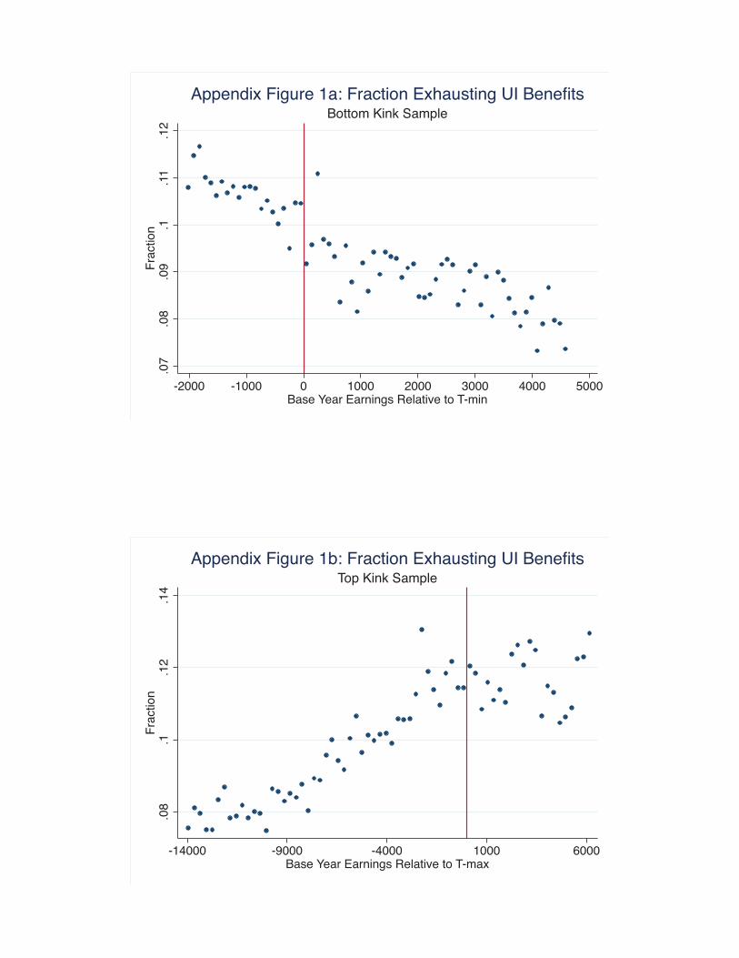
.07
.08
.09
.1.1
1.1
2F
ract
ion
-2000 -1000 0 1000 2000 3000 4000 5000Base Year Earnings Relative to T-min
Bottom Kink SampleAppendix Figure 1a: Fraction Exhausting UI Benefits
.08
.1.1
2.1
4F
ract
ion
-14000 -9000 -4000 1000 6000Base Year Earnings Relative to T-max
Top Kink SampleAppendix Figure 1b: Fraction Exhausting UI Benefits

3232
.533
33.5
3434
.5ag
e in
yea
rs
-2000 -1000 0 1000 2000 3000 4000 5000Base Year Earnings Relative to T-min
Age
.2.3
.4.5
.6ag
e in
yea
rs
-2000 -1000 0 1000 2000 3000 4000 5000Base Year Earnings Relative to T-min
Female
.58
.6.6
2.6
4.6
6.6
8ag
e in
yea
rs
-2000 -1000 0 1000 2000 3000 4000 5000Base Year Earnings Relative to T-min
Bluecollar
.1.1
5.2
.25
age
in y
ears
-2000 -1000 0 1000 2000 3000 4000 5000Base Year Earnings Relative to T-min
Recalled to Last Job
Appendix Figure 2: Covariates Bottom Kink Sample

3536
3738
age
in y
ears
-14000 -9000 -4000 1000 6000Base Year Earnings Relative to T-max
Age
.18
.2.2
2.2
4.2
6ag
e in
yea
rs
-14000 -9000 -4000 1000 6000Base Year Earnings Relative to T-max
Female
.2.3
.4.5
.6.7
age
in y
ears
-14000 -9000 -4000 1000 6000Base Year Earnings Relative to T-max
Bluecollar
.1.1
5.2
.25
.3ag
e in
yea
rs
-14000 -9000 -4000 1000 6000Base Year Earnings Relative to T-max
Recalled to Last Job
Appendix Figure 3: Covariates Top Kink Sample

Appendix Figure 4: Global Relationship between Log Time to Next Job and Baseline Earnings
4.4
4.5
4.6
4.7
0 5000 10000 15000 20000baseline earnings
Bottom kink sampleLog Time to Next Job - Raw Data
-.1-.0
50
.05
.1
0 5000 10000 15000 20000baseline earnings
Bottom kink sampleLog Time to Next Job - Residual
4.4
4.5
4.6
4.7
-20000 -15000 -10000 -5000 0 5000baseline earnings
Top kink sampleLog Time to Next Job - Raw Data
-.1-.0
50
.05
.1
-20000 -15000 -10000 -5000 0 5000baseline earnings
Top kink sampleLog Time to Next Job - Residual
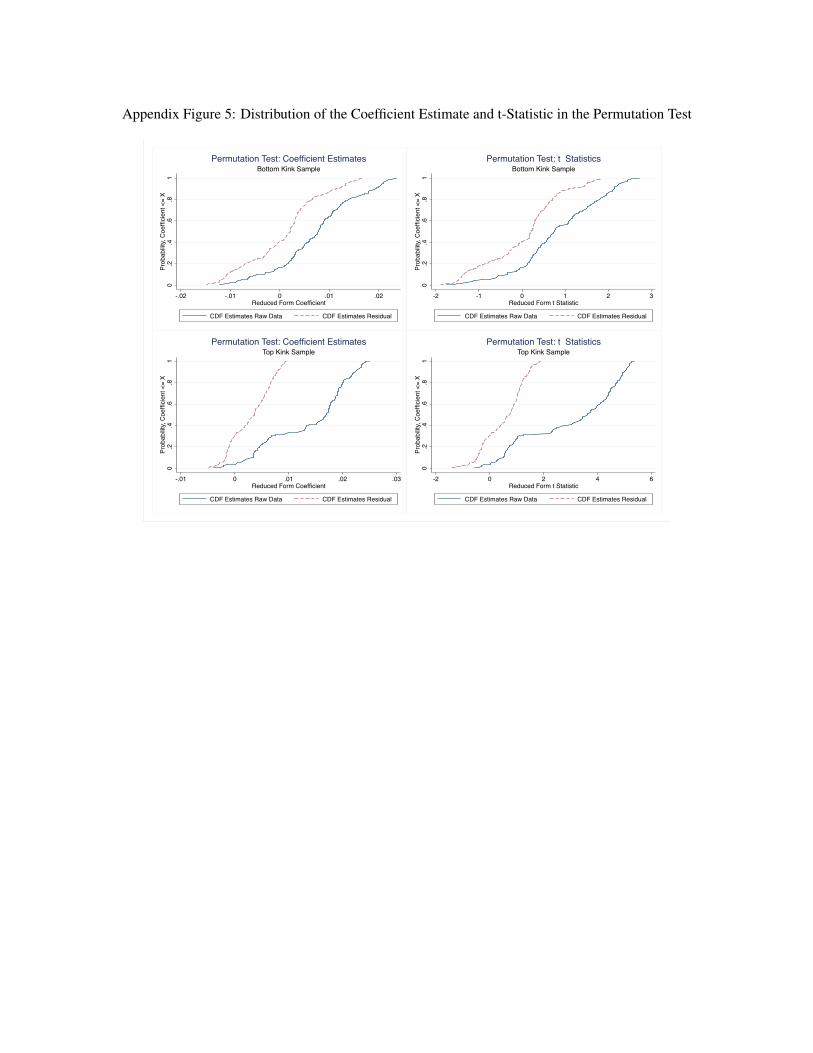
Appendix Figure 5: Distribution of the Coefficient Estimate and t-Statistic in the Permutation Test
0.2
.4.6
.81
Prob
abilit
y, C
oeffi
cien
t <=
X
-.02 -.01 0 .01 .02Reduced Form Coefficient
CDF Estimates Raw Data CDF Estimates Residual
Bottom Kink SamplePermutation Test: Coefficient Estimates
0.2
.4.6
.81
Prob
abilit
y, C
oeffi
cien
t <=
X
-2 -1 0 1 2 3Reduced Form t Statistic
CDF Estimates Raw Data CDF Estimates Residual
Bottom Kink SamplePermutation Test: t Statistics
0.2
.4.6
.81
Prob
abilit
y, C
oeffi
cien
t <=
X
-.01 0 .01 .02 .03Reduced Form Coefficient
CDF Estimates Raw Data CDF Estimates Residual
Top Kink SamplePermutation Test: Coefficient Estimates
0.2
.4.6
.81
Prob
abilit
y, C
oeffi
cien
t <=
X
-2 0 2 4 6Reduced Form t Statistic
CDF Estimates Raw Data CDF Estimates Residual
Top Kink SamplePermutation Test: t Statistics

Appendix Table 1: Testing for Smooth Density of Previous Earnings Using Parametric Models of Frequency
Distributions in Bottom Kink and Top Kink Samples
Estimated Kink x 1000 Pearson χ2 Akaike
(Standard Error) (P‐value) Criterion
(1) (2) (3) (4)
A. Bottom Kink Sample (65 bins of width = 100 Euro/year)
2 0.446 83.02 93.02
(0.172) (2.6%)
3 ‐0.080 73.81 87.81
(0.091) (7.9%)
4 ‐0.240 72.43 90.43
(0.181) (6.9%)
5 0.109 69.39 91.39
(0.308) (7.7%)
B. Top Kink Sample (66 bins of width = 300 Euro/year)
2 ‐0.070 142.55 152.55
(0.035) (0.0%)
3 ‐0.220 124.15 138.15
(0.081) (0.0%)
4 0.200 75.62 93.62
(0.124) (5.0%)
5 0.158 75.50 97.50
(0.213) (3.5%)
Notes: See text. Bottom kink sample includes 254,489 observations (2,803 observations in left‐most and right‐
most bins deleted). Top kink sample includes 271,277 observations (4,388 observations in left‐most and left‐
most bins deleted). Models are estimated by minimum chi‐square. Model for fraction of observations in a bin
is a polynomial function (of the order indicated in column 1) of the bin counter, with interactions of poynomial
terms with indicator for bins to the right of the kink point (main effect of indicator is excluded). Estimated
kink in column 2 is coefficient of interaction between linear term and indicator for bins to right of kinkpoint.
Akaike criterion in column 4 is chi‐squared model fit statistic plus 2 times the number of parameters in the
model.
Polynomial Order of
Model for Histogram

Appendix Table 2a: Summary of Monte Carlo Studies, DGP Design Based on Bottom Kink Sample
(1) (2) (3) (4) (5) (6) (7) (8) (9) (10) (11)1. Local Linear, No Bias CorrectionDefault CCT 470 - 0.31 0.43 0.94 20.3 4.81 1.00 0.72 0.52 22.6CCT, no regularization 998 - 0.04 0.22 0.89 4.7 2.04 0.77 0.68 0.46 3.69Fuzzy CCT 973 - 0.04 0.22 0.89 22.3 1.90 0.77 0.75 0.56 3.06Fuzzy IK 1,415 - 0.00 0.11 0.85 1.60 1.30 0.55 0.83 0.69 1.01FG 2,600 - 0.00 0.08 0.60 1.40 1.35 0.02 1.32 1.75 0.09Global (all data) 4,564 - 0.00 0.14 0.00 1.29 1.25 0.01 1.22 1.49 0.07
2. Local Linear, Bias-CorrectedDefault CCT 470 970 0.60 0.62 0.94 7.0E+02 8.5 1.00 0.71 0.51 71.1CCT, no regularization 998 1,311 0.33 0.47 0.92 10.6 3.96 0.97 0.38 0.14 15.6Fuzzy CCT 973 1,363 0.29 0.45 0.92 1.2E+03 3.76 0.98 0.39 0.16 14.0Fuzzy IK 1,415 1,615 0.21 0.36 0.90 3.84 2.96 0.92 0.31 0.10 8.70FG 2,600 3,367 0.00 0.16 0.89 1.89 1.69 0.82 0.87 0.75 2.10Global (all data) 4,564 4,564 0.00 0.18 0.83 2.17 1.97 0.75 1.54 2.36 1.54
3. Quadratic, No Bias CorrectionDefault CCT 681 - 0.78 0.93 0.95 540 13.5 1.00 -0.38 0.15 183CCT, no regularization 1,211 - 0.38 0.50 0.91 84 6.6 0.98 0.41 0.16 43.2Fuzzy CCT 1,291 - 0.35 0.47 0.91 67 5.6 0.98 0.57 0.32 31.1Fuzzy IK 1,778 - 0.09 0.27 0.90 135 2.77 0.95 0.39 0.15 7.55FG 3,718 - 0.00 0.14 0.88 2.12 1.90 0.72 1.27 1.60 2.00Global (all data) 4,564 - 0.00 0.17 0.76 2.56 2.39 0.54 2.13 4.54 1.15
4. Local Quadratic, Bias-CorrectedDefault CCT 681 1,079 0.85 1.25 0.95 703252 22.4 1.00 1.03 1.07 499CCT, no regularization 1,211 1,384 0.76 1.02 0.92 2.2E+04 13.2 1.00 0.48 0.23 175Fuzzy CCT 1,291 1,462 0.76 1.00 0.94 4058 12.8 0.99 0.38 0.15 165Fuzzy IK 1,778 1,657 0.73 1.21 0.92 5.2E+05 10.6 0.96 0.55 0.30 113FG 3,718 4,945 0.24 0.37 0.90 3.54 3.00 0.95 -0.01 0.00 9.03Global (all data) 4,564 4,564 0.24 0.37 0.89 3.67 3.11 0.95 -0.01 0.00 9.70
Notes: based on 1,000 simulations. DGP is based on 5th order polynomial approximation of top kink sample. True kink in first stage is: -1.4 × 10⁻⁵ . True elasticity is: 0. The trimmed statistic are obtained by first trimming the 5% sample in which the estimates deviate the most from the true parameter value.
Bias (trimmed)
Bias2
(trimmed)Variance
(trimmed)
C.I. Coverage
RateRMSE RMSE
(trimmed)
C.I. Coverage
Rate
Elasticity Estimation Summary
Median Main b.w.
Median Pilot b.w.
First Stage Model Estimation SummaryFraction of
Replications: C.I. includes 0
RMSE/true value
(trimmed)
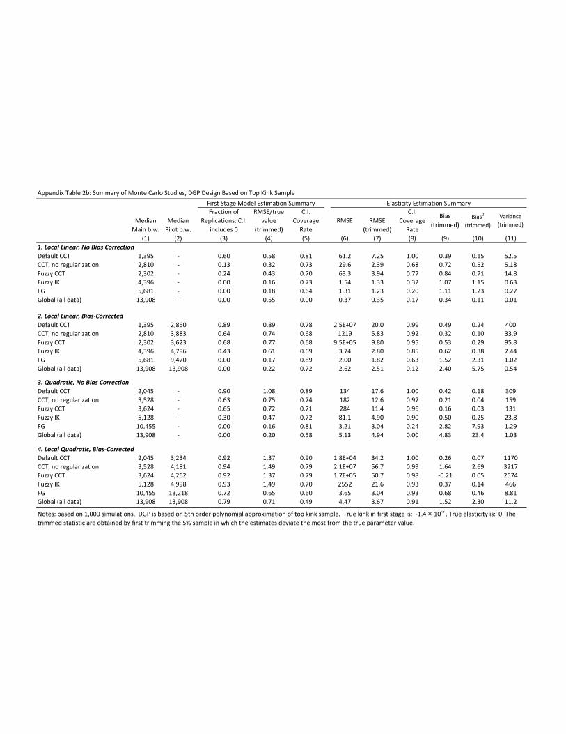
Appendix Table 2b: Summary of Monte Carlo Studies, DGP Design Based on Top Kink Sample
(1) (2) (3) (4) (5) (6) (7) (8) (9) (10) (11)1. Local Linear, No Bias CorrectionDefault CCT 1,395 - 0.60 0.58 0.81 61.2 7.25 1.00 0.39 0.15 52.5CCT, no regularization 2,810 - 0.13 0.32 0.73 29.6 2.39 0.68 0.72 0.52 5.18Fuzzy CCT 2,302 - 0.24 0.43 0.70 63.3 3.94 0.77 0.84 0.71 14.8Fuzzy IK 4,396 - 0.00 0.16 0.73 1.54 1.33 0.32 1.07 1.15 0.63FG 5,681 - 0.00 0.18 0.64 1.31 1.23 0.20 1.11 1.23 0.27Global (all data) 13,908 - 0.00 0.55 0.00 0.37 0.35 0.17 0.34 0.11 0.01
2. Local Linear, Bias-CorrectedDefault CCT 1,395 2,860 0.89 0.89 0.78 2.5E+07 20.0 0.99 0.49 0.24 400CCT, no regularization 2,810 3,883 0.64 0.74 0.68 1219 5.83 0.92 0.32 0.10 33.9Fuzzy CCT 2,302 3,623 0.68 0.77 0.68 9.5E+05 9.80 0.95 0.53 0.29 95.8Fuzzy IK 4,396 4,796 0.43 0.61 0.69 3.74 2.80 0.85 0.62 0.38 7.44FG 5,681 9,470 0.00 0.17 0.89 2.00 1.82 0.63 1.52 2.31 1.02Global (all data) 13,908 13,908 0.00 0.22 0.72 2.62 2.51 0.12 2.40 5.75 0.54
3. Quadratic, No Bias CorrectionDefault CCT 2,045 - 0.90 1.08 0.89 134 17.6 1.00 0.42 0.18 309CCT, no regularization 3,528 - 0.63 0.75 0.74 182 12.6 0.97 0.21 0.04 159Fuzzy CCT 3,624 - 0.65 0.72 0.71 284 11.4 0.96 0.16 0.03 131Fuzzy IK 5,128 - 0.30 0.47 0.72 81.1 4.90 0.90 0.50 0.25 23.8FG 10,455 - 0.00 0.16 0.81 3.21 3.04 0.24 2.82 7.93 1.29Global (all data) 13,908 - 0.00 0.20 0.58 5.13 4.94 0.00 4.83 23.4 1.03
4. Local Quadratic, Bias-CorrectedDefault CCT 2,045 3,234 0.92 1.37 0.90 1.8E+04 34.2 1.00 0.26 0.07 1170CCT, no regularization 3,528 4,181 0.94 1.49 0.79 2.1E+07 56.7 0.99 1.64 2.69 3217Fuzzy CCT 3,624 4,262 0.92 1.37 0.79 1.7E+05 50.7 0.98 -0.21 0.05 2574Fuzzy IK 5,128 4,998 0.93 1.49 0.70 2552 21.6 0.93 0.37 0.14 466FG 10,455 13,218 0.72 0.65 0.60 3.65 3.04 0.93 0.68 0.46 8.81Global (all data) 13,908 13,908 0.79 0.71 0.49 4.47 3.67 0.91 1.52 2.30 11.2
Notes: based on 1,000 simulations. DGP is based on 5th order polynomial approximation of top kink sample. True kink in first stage is: -1.4 × 10⁻⁵ . True elasticity is: 0. The trimmed statistic are obtained by first trimming the 5% sample in which the estimates deviate the most from the true parameter value.
Bias (trimmed)
Bias2
(trimmed)Variance
(trimmed)
C.I. Coverage
RateRMSE RMSE
(trimmed)
C.I. Coverage
Rate
Elasticity Estimation Summary
Median Main b.w.
Median Pilot b.w.
First Stage Model Estimation SummaryFraction of
Replications: C.I. includes 0
RMSE/true value
(trimmed)

Appendix Table 3: Estimated AMSE for Local Linear and Local Quadratic Models Default CCT bandwidth
AMSE Variance Bias2 AMSE Variance Bias2
(1) (2) (3) (4) (5) (6)
Bottom Kink 12.51 12.47 0.04 2434 2406 28
Top Kink 3.98 3.17 0.81 20.41 18.98 1.43
Table entries are estimates of AMSE for the local linear and local quadratic estimators under the default CCT bandwidth, with asymptotic variance and asymptotic squared bias components.
Local Linear Local Quadratic

App
endi
xTa
ble
4:Su
mm
ary
ofE
stim
ated
Ben
efitE
last
iciti
esin
Exi
stin
gL
itera
ture
Aut
hors
(dat
e)D
ata
Des
ign
Ela
stic
ityE
stim
ate
orR
ange
U.S
.Stu
dies
Cla
ssen
(197
7b)
CW
BH
*,A
rizo
naPr
e/po
st,R
KD
0.6
-1.0
Mof
fitt(
1985
)C
WB
H,1
3st
ates
Cro
ss-s
ectio
nal
0.4
Solo
n(1
985)
CW
BH
,Geo
rgia
Diff
-in-
diff
,tax
polic
ych
ange
0.7
Mey
er(1
990)
CW
BH
,all
stat
esSt
ate-
by-y
ear
0.8
Kat
zan
dM
eyer
(199
0)C
WB
H,a
llst
ates
Stat
e-by
-yea
r0.
8M
eyer
and
Mok
(200
7)N
ewY
ork
Stat
eU
IRec
ords
Pre/
post
0.3
Che
tty(2
010)
SIPP
(ret
rosp
ectiv
ein
terv
iew
s)St
ate-
by-y
ear
0.5
Lan
dais
(For
thco
min
g)C
WB
H,L
ouis
iana
/Was
hing
ton
RK
D,m
axim
umbe
nefit
0.2-
0.7
Eur
opea
nSt
udie
sC
arlin
get
al.(
2011
)Sw
eden
,reg
iste
rdat
aD
iff-i
n-di
ff,r
epl.
rate
chan
ge1.
6(o
utco
me
=tim
eto
next
job)
Roe
dan
dZ
hang
(200
3)N
orw
ay,r
egis
terd
ata,
prev
ious
Cal
enda
rvs.
spel
ldat
ing
0.3
(fem
ale)
job
<2
year
s0.
9(m
ale)
Lal
ive
etal
.(20
06)
Aus
tria
,reg
iste
r/So
cial
Secu
rity
data
Diff
-in-
diff
,rep
l.ra
tech
ange
0.15
Arr
azet
al.(
2008
)Sp
ain,
regi
ster
data
Pre/
post
0.8
*N
ote:
CW
BH
isth
eC
ontin
uous
Wor
kan
dB
enefi
tHis
tory
data
set,
base
don
empl
oym
enta
ndun
empl
oym
entr
ecor
ds.