recommendations for the quantitative analysis of landslide ... · recommendations for the...

ORIGINAL PAPER

Recommendations for the quantitative analysis of landslide risk

J. Corominas • C. van Westen • P. Frattini • L. Cascini • J.-P. Malet •

S. Fotopoulou • F. Catani • M. Van Den Eeckhaut • O. Mavrouli •

F. Agliardi • K. Pitilakis • M. G. Winter • M. Pastor • S. Ferlisi • V. Tofani •

J. Hervas • J. T. Smith

Received: 4 June 2013 / Accepted: 11 October 2013 / Published online: 24 November 2013

� The Author(s) 2013. This article is published with open access at Springerlink.com

Abstract This paper presents recommended methodolo-

gies for the quantitative analysis of landslide hazard, vul-

nerability and risk at different spatial scales (site-specific,

local, regional and national), as well as for the verification

and validation of the results. The methodologies described

focus on the evaluation of the probabilities of occurrence of

different landslide types with certain characteristics.

Methods used to determine the spatial distribution of

landslide intensity, the characterisation of the elements at

risk, the assessment of the potential degree of damage and

the quantification of the vulnerability of the elements at

risk, and those used to perform the quantitative risk ana-

lysis are also described. The paper is intended for use by

scientists and practising engineers, geologists and other

landslide experts.

Keywords Landslides � Risk � Hazard �Vulnerability � Susceptibility � Methodology for

quantitative analysis � Rockfalls � Debris flow �Slow-moving landslides

Introduction

Despite considerable improvements in our understanding

of instability mechanisms and the availability of a wide

J. Corominas (&) � O. Mavrouli

Department of Geotechnical Engineering and Geosciences,

Technical University of Catalonia, 08034 Barcelona, Spain

e-mail: [email protected]

C. van Westen

Faculty of Geo-information Sciences and Earth Observation,

University of Twente, 7500 AE Enschede, The Netherlands

P. Frattini � F. Agliardi

Department of Earth and Environmental Science, Universita

degli Studi di Milano-Bicocca, 20126 Milan, Italy

L. Cascini � S. Ferlisi

Department of Civil Engineering, University of Salerno,

84084 Salerno, Italy

J.-P. Malet

Centre National de la Recherche Scientifique, Institut de

Physique du Globe de Strasbourg, 67084 Strasbourg, France

S. Fotopoulou � K. Pitilakis

Research Unit of Geotechnical Earthquake Engineering and Soil

Dynamics, Department of Civil Engineering, Aristotle

University of Thessaloniki, 54124 Thessaloniki, Greece

F. Catani � V. Tofani

Department of Earth Sciences, University of Firenze,

50121 Florence, Italy

M. Van Den Eeckhaut � J. Hervas

Institute for Environment and Sustainability, Joint Research

Centre, European Commission, 21027 Ispra, Italy

M. G. Winter

Transport Research Laboratory (TRL), 13 Swanston Steading,

109 Swanston Road, Edinburgh EH10 7DS, UK

M. Pastor

ETS Ingenieros de Caminos, Universidad Politecnica de Madrid,

28071 Madrid, Spain

J. T. Smith

Golder Associates (formerly TRL), Cavendish House, Bourne

End Business Park, Cores End Road, Bourne End SL8 8AS, UK

123

Bull Eng Geol Environ (2014) 73:209–263

DOI 10.1007/s10064-013-0538-8

range of mitigation techniques, landslides still cause a

significant death toll and significant economic losses all

over the world. Recent studies (Petley 2012) have shown

that loss of life is concentrated in less developed countries,

where there is relatively little investment in understanding

the hazards and risks associated with landslides, due lar-

gely to a lack of appropriate resources. Cooperative

research and greater capacity-building efforts are required

to support the local and regional administrations which are

in charge of landslide risk management in most of the

countries.

Authorities and decision makers need maps depicting

the areas that may be affected by landslides so that they are

considered in development plans and/or that appropriate

risk mitigation measures are implemented. A wide variety

of methods for assessing landslide susceptibility, hazard

and risk are available and, to assist in risk management

decisions, several institutions and scientific societies have

proposed guidelines for the preparation of landslide hazard

maps (i.e. OFAT, OFEE, OFEFP 1997; GEO 2006; AGS

2007; Fell et al. 2008a, b), with the common goal being to

use a unified terminology and highlight the fundamental

data needed to prepare the maps and guide practitioners in

their analyses. Some of them are intended to be introduced

into legislated standards (OFAT, OFEE, OFEFP 1997;

AGS 2007). However, the methodologies implemented

diverge significantly from country to country, and even

within the same country (Corominas et al. 2010).

To manage risk, it must be first analysed and evaluated.

The landslide risk for an object or an area must be calcu-

lated with reference to a given time frame for which the

expected frequency or probability of occurrence of an

event of intensity higher than a minimum established value

is evaluated. In that respect, there is an increasing need to

perform quantitative risk analysis (QRA). QRA is distin-

guished from qualitative risk analysis by the input data, the

procedures used in the analysis and the final risk output. In

contrast with qualitative risk analysis, which yields results

in terms of weighted indices, relative ranks (e.g. low,

moderate and high) or numerical classification, QRA

quantifies the probability of a given level of loss and the

associated uncertainties.

QRA is important for scientists and engineers because it

allows risk to be quantified in an objective and reproduc-

ible manner, and the results can be compared from one

location (site, region, etc.) to another. Furthermore, it helps

with the identification of gaps in the input data and the

understanding of the weaknesses of the analyses used. For

landslide risk managers, it is also useful because it allows a

cost–benefit analysis to be performed, and it provides the

basis for the prioritisation of management and mitigation

actions and the associated allocation of resources. For

society in general, QRA helps to increase the awareness of

existing risk levels and the appreciation of the efficacy of

the actions undertaken.

For QRA, more accurate geological and geomechanical

input data and a high-quality DEM are usually necessary to

evaluate a range of possible scenarios, design events and

return periods. Lee and Jones (2004) warned that the

probability of landsliding and the value of adverse conse-

quences are only estimates. Due to limitations in the

available information, the use of numbers may conceal the

fact that the potential for error is great. In that respect,

QRA is not necessarily more objective than the qualitative

estimations, as, for example, probability may be estimated

based on personal judgment. It does, however, facilitate

communication between geoscience professionals, land

owners and decision makers.

Risk for a single landslide scenario may be expressed

analytically as follows:

R ¼ PðMiÞP XjjMi

� �P T jXj

� �VijC; ð1Þ

where R is the risk due to the occurrence of a landslide of

magnitude Mi on an element at risk located at a distance

X from the landslide source, P(Mi) is the probability of

occurrence of a landslide of magnitude Mi, P(Xj|Mi) is the

probability of the landslide reaching a point located at a

distance X from the landslide source with an intensity j,

P(T|Xj) is the probability of the element being at the point

X at the time of occurrence of the landslide, Vij is the

vulnerability of the element to a landslide of magnitude

i and intensity j, and C is the value of the element at risk.

Three basic components appear in Eq. 1 that must be

specifically considered in the assessment: the hazard, the

exposure of the elements at risk, and their vulnerability.

They are characterised by both spatial and nonspatial

attributes. Landslide hazard is characterised by its proba-

bility of occurrence and intensity (see the ‘‘Landslide

hazard assessment’’ section); the latter expresses the

severity of the hazard. The elements at risk are the popu-

lation, property, economic activities, including public ser-

vices, or any other defined entities exposed to hazards in a

given area (UN-ISDR 2004). The elements at risk also have

spatial and nonspatial characteristics. The interaction of

hazard and the elements at risk involves the exposure and

the vulnerability of the latter. Exposure indicates the extent

to which the elements at risk are actually located in the

path of a particular landslide. Vulnerability refers to the

conditions, as determined by physical, social, economic

and environmental factors or processes, which make a

community susceptible to the impact of hazards (UN-ISDR

2004). Physical vulnerability is evaluated as the interaction

between the intensity of the hazard and the type of ele-

ments at risk, making use of so-called vulnerability curves

(see ‘‘Vulnerability assessment’’ section). For further

explanations of hazard and risk analysis, the reader is

210 J. Corominas et al.

123

referred to textbooks such as Lee and Jones (2004), Glade

et al. (2005) and Smith and Petley (2008).

Probably the most critical issue is the determination of

the temporal occurrence of landslides. In many regions, a

lack of data prevents the performance of a quantitative

determination of the probability of slope failure or land-

slide reactivation within a defined time span. Despite this

limitation, landslide risk management decisions are some-

times taken considering the spatial distribution of existing

or potential landslides. This is carried out by means of the

analysis of the landslide predisposing factors or suscepti-

bility analysis (see the ‘‘Suggested methods for landslide

susceptibility assessment’’ section).

The goal of these recommendations is to present an

overview of the existing methodologies for the quantitative

analysis and zoning of landslide susceptibility, hazard and

risk at different scales, and to provide guidance on how to

implement them. They are not intended to become stan-

dards. The aim is to provide a selection of quantitative

tools to researchers and practitioners involved in landslide

hazard and risk analysis, and mapping procedures. Users

must be aware of the information and tasks required to

characterise the landslide areas, to assess the hazard level,

and to evaluate the potential risks as well as the associated

uncertainties.

The paper is structured similarly to the JTC-1 Guide-

lines (Fell et al. 2008a, b); indeed, some of the authors

were deeply involved in the preparation of those Guide-

lines. However, all of the sections have been updated. The

sections ‘‘QRA framework’’, ‘‘Landslide zoning at differ-

ent scales’’, and ‘‘Input data for landslide risk analysis’’

describe the framework of the QRA and its main compo-

nents; the requirements associated with the scale of work as

well as the hazard and risk descriptors; and the input data

and their sources. The sections ‘‘Suggested methods for

landslide susceptibility assessment’’, ‘‘Landslide hazard

assessment’’, and ‘‘Suggested methods for quantitative

landslide risk analysis’’ discuss, respectively, the available

methods for quantifying and mapping landslide suscepti-

bility, hazard and risk. Finally, the ‘‘Evaluation of the

performance of landslide zonation maps’’ section presents

procedures to check the reliability of the maps and validate

the results. At the end of the document, an ‘‘Appendix’’

section is included with basic definitions of the terms used.

These recommendations focus on quantitative approa-

ches only. Significant efforts have been made to expound

on topics that were only marginally treated in previously

published guidelines, and this sometimes required novel

developments: (a) the procedures for preparing landslide

hazard maps from susceptibility maps; (b) the analysis of

hazards from multiple landslide types; (c) the assessment

of the exposure of the elements at risk; (d) the assessment

of the vulnerability, particularly the physical vulnerability

and the construction of vulnerability curves; and (e) the

verification of the models and the validation of the land-

slide maps.

QRA framework

The general framework involves the complete process of

risk assessment and risk control (or risk treatment). Risk

assessment includes the process of risk analysis and risk

evaluation. Risk analysis uses available information to

estimate the risk to individuals, population, property or the

environment from hazards. Risk analysis generally con-

tains the following steps: hazard identification, hazard

assessment, inventory of elements at risk and exposure,

vulnerability assessment and risk estimation. Since all of

these steps have an important spatial component, risk

analysis often requires the management of a set of spatial

data and the use of geographic information systems. Risk

evaluation is the stage at which values and judgments enter

the decision process, explicitly or implicitly, including

considerations of the importance of the estimated risks and

the associated social, environmental, and economic con-

sequences, in order to identify a range of alternatives for

managing the risks.

Landslide hazard assessment requires a multi-hazard

approach, as different types of landslides may occur, each

with different characteristics and causal factors, and with

different spatial, temporal and size probabilities. Also,

landslide hazards often occur in conjunction with other

types of hazards (e.g. flooding or earthquakes). Figure 1,

based on Van Westen et al. (2005), gives the framework of

multi-hazard landslide risk assessment, with an indication

of the various steps (A–H). The first step (A) deals with the

input data required for a multi-hazard risk assessment,

focussing on the data needed to generate susceptibility

maps for initiation and runout, triggering factors, multi-

temporal inventories and elements at risk.

The second step (B) focuses on susceptibility assess-

ment, and is divided into two components. The first, which

is the most frequently used, deals with the modelling of

potential initiation areas (initiation susceptibility), which

can make use of a variety of different methods (inventory-

based, heuristic, statistical, deterministic), which will be

discussed later in this document. The resulting maps will

display the source areas for the modelling of potential

runout areas (reach probability).

The third step (C) deals with landslide hazard

assessment, which heavily depends on the availability of

so-called event-based landslide inventories, which are

inventories of landslides caused by the same triggering

event. By linking landslide distributions to the temporal

probability of the triggering event, it is possible to carry

Quantitative analysis of landslide risk 211

123

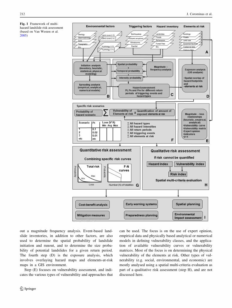
out a magnitude frequency analysis. Event-based land-

slide inventories, in addition to other factors, are also

used to determine the spatial probability of landslide

initiation and runout, and to determine the size proba-

bility of potential landslides for a given return period.

The fourth step (D) is the exposure analysis, which

involves overlaying hazard maps and elements-at-risk

maps in a GIS environment.

Step (E) focuses on vulnerability assessment, and indi-

cates the various types of vulnerability and approaches that

can be used. The focus is on the use of expert opinion,

empirical data and physically based analytical or numerical

models in defining vulnerability classes, and the applica-

tion of available vulnerability curves or vulnerability

matrices. Most of the focus is on determining the physical

vulnerability of the elements at risk. Other types of vul-

nerability (e.g. social, environmental, and economic) are

mostly analysed using a spatial multi-criteria evaluation as

part of a qualitative risk assessment (step H), and are not

discussed here.

Fig. 1 Framework of multi-

hazard landslide risk assessment

(based on Van Westen et al.

2005)


123

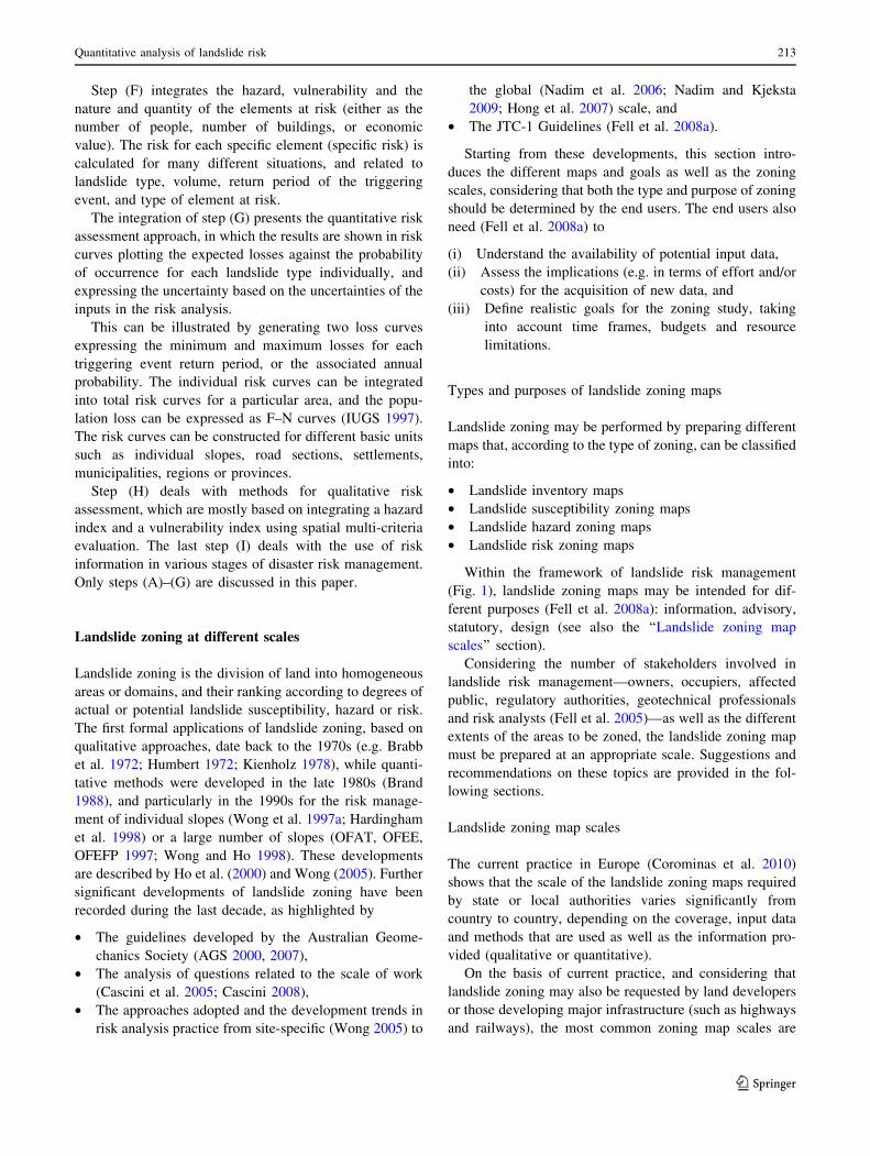
Step (F) integrates the hazard, vulnerability and the

nature and quantity of the elements at risk (either as the

number of people, number of buildings, or economic

value). The risk for each specific element (specific risk) is

calculated for many different situations, and related to

landslide type, volume, return period of the triggering

event, and type of element at risk.

The integration of step (G) presents the quantitative risk

assessment approach, in which the results are shown in risk

curves plotting the expected losses against the probability

of occurrence for each landslide type individually, and

expressing the uncertainty based on the uncertainties of the

inputs in the risk analysis.

This can be illustrated by generating two loss curves

expressing the minimum and maximum losses for each

triggering event return period, or the associated annual

probability. The individual risk curves can be integrated

into total risk curves for a particular area, and the popu-

lation loss can be expressed as F–N curves (IUGS 1997).

The risk curves can be constructed for different basic units

such as individual slopes, road sections, settlements,

municipalities, regions or provinces.

Step (H) deals with methods for qualitative risk

assessment, which are mostly based on integrating a hazard

index and a vulnerability index using spatial multi-criteria

evaluation. The last step (I) deals with the use of risk

information in various stages of disaster risk management.

Only steps (A)–(G) are discussed in this paper.

Landslide zoning at different scales

Landslide zoning is the division of land into homogeneous

areas or domains, and their ranking according to degrees of

actual or potential landslide susceptibility, hazard or risk.

The first formal applications of landslide zoning, based on

qualitative approaches, date back to the 1970s (e.g. Brabb

et al. 1972; Humbert 1972; Kienholz 1978), while quanti-

tative methods were developed in the late 1980s (Brand

1988), and particularly in the 1990s for the risk manage-

ment of individual slopes (Wong et al. 1997a; Hardingham

et al. 1998) or a large number of slopes (OFAT, OFEE,

OFEFP 1997; Wong and Ho 1998). These developments

are described by Ho et al. (2000) and Wong (2005). Further

significant developments of landslide zoning have been

recorded during the last decade, as highlighted by

• The guidelines developed by the Australian Geome-

chanics Society (AGS 2000, 2007),

• The analysis of questions related to the scale of work

(Cascini et al. 2005; Cascini 2008),

• The approaches adopted and the development trends in

risk analysis practice from site-specific (Wong 2005) to

the global (Nadim et al. 2006; Nadim and Kjeksta

2009; Hong et al. 2007) scale, and

• The JTC-1 Guidelines (Fell et al. 2008a).

Starting from these developments, this section intro-

duces the different maps and goals as well as the zoning

scales, considering that both the type and purpose of zoning

should be determined by the end users. The end users also

need (Fell et al. 2008a) to

(i) Understand the availability of potential input data,

(ii) Assess the implications (e.g. in terms of effort and/or

costs) for the acquisition of new data, and

(iii) Define realistic goals for the zoning study, taking

into account time frames, budgets and resource

limitations.

Types and purposes of landslide zoning maps

Landslide zoning may be performed by preparing different

maps that, according to the type of zoning, can be classified

into:

• Landslide inventory maps

• Landslide susceptibility zoning maps

• Landslide hazard zoning maps

• Landslide risk zoning maps

Within the framework of landslide risk management

(Fig. 1), landslide zoning maps may be intended for dif-

ferent purposes (Fell et al. 2008a): information, advisory,

statutory, design (see also the ‘‘Landslide zoning map

scales’’ section).

Considering the number of stakeholders involved in

landslide risk management—owners, occupiers, affected

public, regulatory authorities, geotechnical professionals

and risk analysts (Fell et al. 2005)—as well as the different

extents of the areas to be zoned, the landslide zoning map

must be prepared at an appropriate scale. Suggestions and

recommendations on these topics are provided in the fol-

lowing sections.

Landslide zoning map scales

The current practice in Europe (Corominas et al. 2010)

shows that the scale of the landslide zoning maps required

by state or local authorities varies significantly from

country to country, depending on the coverage, input data

and methods that are used as well as the information pro-

vided (qualitative or quantitative).

On the basis of current practice, and considering that

landslide zoning may also be requested by land developers

or those developing major infrastructure (such as highways

and railways), the most common zoning map scales are


123

described hereafter, together with some considerations

regarding the outputs and pursued purposes.

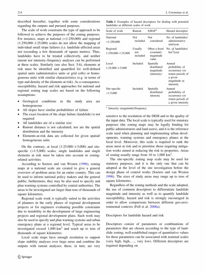
The scale of work constrains the type of approach to be

followed to achieve the purposes of the zoning purposes.

For instance, maps at national (\1:250,000) and regional

(1:250,000–1:25,000) scales do not allow the mapping of

individual small slope failures (i.e. landslide-affected areas

not exceeding a few thousands of square metres). Thus,

landslides have to be treated collectively, and neither

runout nor intensity–frequency analyses can be performed

at these scales. Similarly (see also Sect. 5.6), elements at

risk must be identified and quantified for well-defined

spatial units (administrative units or grid cells) or homo-

geneous units with similar characteristics (e.g. in terms of

type and density of the elements at risk). As a consequence,

susceptibility, hazard and risk approaches for national and

regional zoning map scales are based on the following

assumptions:

• Geological conditions in the study area are

homogeneous

• All slopes have similar probabilities of failure

• The exact location of the slope failure (landslide) is not

required

• All landslides are of a similar size

• Runout distance is not calculated; nor are the spatial

distribution and the intensity

• Elements-at-risk data are collected for given spatial/

homogeneous units

On the contrary, at local (1:25,000–1:5,000) and site-

specific ([1:5,000) scales, single landslides and single

elements at risk must be taken into account in zoning-

related activities.

According to Soeters and van Westen (1996), zoning

maps at a national scale are created to give a general

overview of problem areas for an entire country. This can

be used to inform national policy makers and the general

public; furthermore, they may be also used to specify and

plan warning systems controlled by central authorities. The

areas to be investigated are larger than tens of thousands of

square kilometres.

Regional scale work is typically suited to the activities

of planners in the early phases of regional development

projects or for engineers evaluating possible constraints

due to instability in the development of large engineering

projects and regional development plans. Such work may

also be used to specify and plan warning systems and urban

emergency plans at a regional level. Typical areas to be

investigated exceed 1,000 km2 and reach up to tens of

thousands of square kilometres.

Local scale maps have enough resolution to support

slope stability analyses over large areas and combine the

outputs with runout analyses; these, in turn, are very

sensitive to the resolution of the DEM and to the quality of

the input data. The local scale is typically used for statutory

purposes (the zoning maps may be legally binding for

public administrators and land users), and it is the reference

scale used when planning and implementing urban devel-

opments, warning systems and emergency planes at the

local level. Moreover, this scale is required to rank the

areas most at risk and to prioritise those requiring mitiga-

tion works aimed at reducing the risk to properties. Areas

of zoning usually range from 10 to 1,000 km2.

The site-specific zoning map scale may be used for

statutory purposes, and it is the only one that can be

adopted at the level of the site investigation before the

design phase of control works (Soeters and van Westen

1996). The sizes of study areas may range up to tens of

square kilometres.

Regardless of the zoning methods and the scale adopted,

the use of common descriptors to differentiate landslide

magnitude and intensity as well as to quantify landslide

susceptibility, hazard and risk is strongly encouraged in

order to allow comparisons between different geo-envi-

ronmental contexts (Fell et al. 2008a).

Descriptors for landslide hazard and risk

Descriptors consist of parameters or combinations of

parameters that are chosen according to the type of land-

slide zoning; well-established ranges of quantitative values

for these parameters can be associated with nominal scales

(very high, high,…., very low). Different descriptors are

required depending on

Table 1 Examples of hazard descriptors for dealing with potential

landslides at different scales of work

Scale of work Runout I(M)/Fa Hazard descriptor

National

\1:250,000

Not

included

Not

considered

No. of landslides/

administrative

unit/year

Regional

1:250,000–1:25,000

Usually

not

included

Often a fixed

(constant)

magnitude

value

No. of landslides/

km2/year

Local

1:25,000–1:5,000

Included Spatially

distributed

magnitude

(intensity)

Annual

probability of

occurrence (or

return period) of

a given

magnitude or

intensity

Site-specific

[1:5,000

Included Spatially

distributed

intensity

Annual

probability of

occurrence (or

return period) of

a given intensity

a Intensity (magnitude)/frequency


123

• The scale of analysis (the mapping units adopted for the

national scale may be different to those adopted at the

site-specific scale) and the related zoning purposes

(information, advisory, statutory and design)

• The landslide type (potential or existing) and the

characteristics of the landslides (e.g. magnitude)

• The characteristics of the exposed elements (e.g. linear

infrastructures, urbanised areas, other)

• The adopted risk acceptability/tolerability criteria,

which may vary from country to country (Leroi et al.

2005).

Table 1 provides examples of landslide hazard

descriptors that should be considered in zoning activity.

Input data for landslide risk analysis

This section reviews the input data required for assessing

landslide susceptibility, hazard and risk. Taking into

account the huge amount of literature on this topic, a

summary will be given of the parameters that are most

suitable for analysing the occurrence of, and the potential

for, different landslide mechanisms (rockfalls, shallow

landslides and debris flows, and slow-moving large land-

slides). The main data layers required for landslide sus-

ceptibility, hazard and risk analysis can be subdivided into

four groups: landslide inventory data, environmental fac-

tors, triggering factors and elements at risk (Soeters and

van Westen 1996; Van Westen et al. 2008). Of these, the

landslide inventory is the most important, as it gives insight

in the location of past landslide occurrences, as well as

their failure mechanisms, causal factors, frequency of

occurrence, volumes and the damage that has been caused.

Parameters controlling the occurrence of landslides

The occurence and frequency–magnitude of mass move-

ments are controlled by a large number of factors, which

can be subdivided into intrinsic, or predisposing, factors

that contribute to the instability of the slope and the factors

that actually trigger the event. The type and weighting of

each factor depends on the environmental setting (e.g.

climatic conditions, internal relief, geological setting,

geomorphological evolution and processes) and may also

differ substantially within a given area due to subtle dif-

ferences in terrain conditions (e.g. soil properties and

depth, subsurface hydrology, density and orientation of

discontinuities, local relief). Different combinations of

factors may control different types of landslides within the

same area. A recent overview of landslide mechanisms and

triggers is presented by Crosta et al. (2012). They provide a

detailed description of the different landslide triggers, such

as rainfall and changes in slope hydrology, changes in

slope geometry due to excavation or erosion, earthquakes

and related dynamic actions, snowmelt and permafrost

degradation, deglaciation and related processes in the

paraglacial environment, rock/soil weathering and related

degradation, volcanic processes, and human activity.

The large diversity in predisposing and triggering fac-

tors complicates the analysis of landslide susceptibility and

hazard, for which the methods and approaches, and the data

required, differ from case to case. Also, the scale at which

the analysis takes place plays an important role. Glade and

Crozier (2005) present a discussion of the relation between

data availability, model complexity and predictive capac-

ity. It is not possible to provide strict guidelines on the type

of data required for a landslide hazard and risk analysis in

the form of a prescribed uniform list of predisposing and

triggering factors. The selection of causal factors differs

depending on the scale of analysis, the characteristics of

the study area, the landslide type, and the failure mecha-

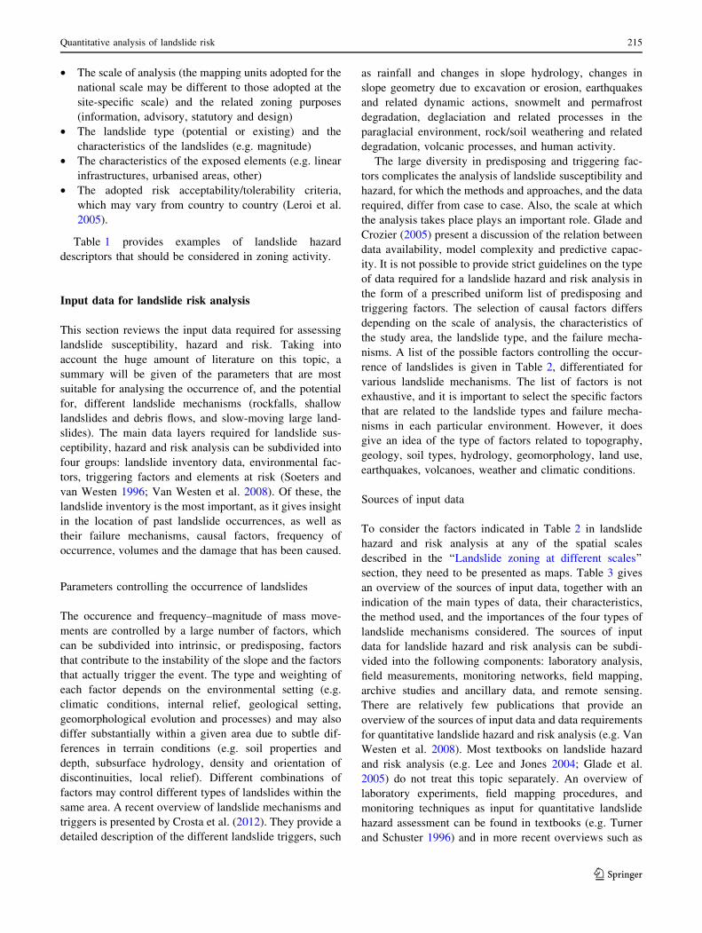
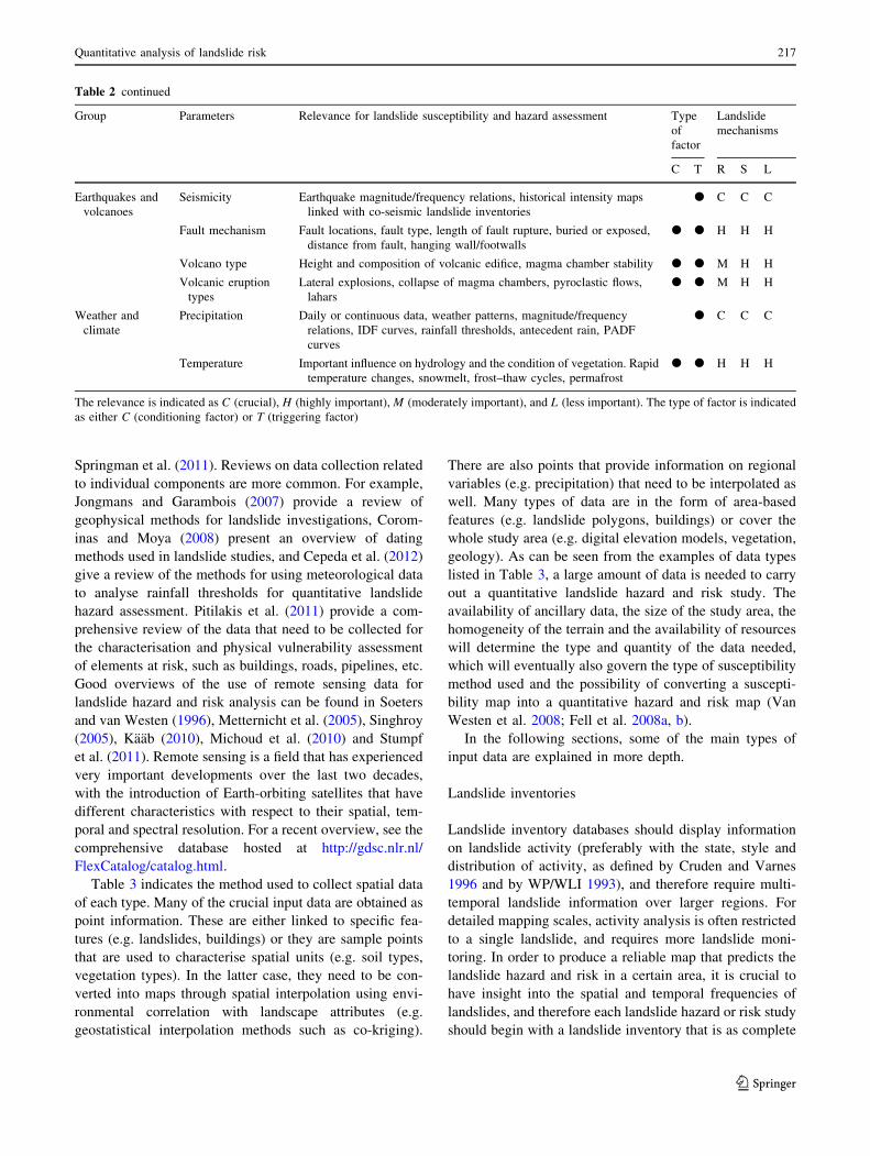
nisms. A list of the possible factors controlling the occur-

rence of landslides is given in Table 2, differentiated for

various landslide mechanisms. The list of factors is not

exhaustive, and it is important to select the specific factors

that are related to the landslide types and failure mecha-

nisms in each particular environment. However, it does

give an idea of the type of factors related to topography,

geology, soil types, hydrology, geomorphology, land use,

earthquakes, volcanoes, weather and climatic conditions.

Sources of input data

To consider the factors indicated in Table 2 in landslide

hazard and risk analysis at any of the spatial scales

described in the ‘‘Landslide zoning at different scales’’

section, they need to be presented as maps. Table 3 gives

an overview of the sources of input data, together with an

indication of the main types of data, their characteristics,

the method used, and the importances of the four types of

landslide mechanisms considered. The sources of input

data for landslide hazard and risk analysis can be subdi-

vided into the following components: laboratory analysis,

field measurements, monitoring networks, field mapping,

archive studies and ancillary data, and remote sensing.

There are relatively few publications that provide an

overview of the sources of input data and data requirements

for quantitative landslide hazard and risk analysis (e.g. Van

Westen et al. 2008). Most textbooks on landslide hazard

and risk analysis (e.g. Lee and Jones 2004; Glade et al.

2005) do not treat this topic separately. An overview of

laboratory experiments, field mapping procedures, and

monitoring techniques as input for quantitative landslide

hazard assessment can be found in textbooks (e.g. Turner

and Schuster 1996) and in more recent overviews such as


123

Table 2 Overview of factors controlling the occurrence of landslides, and their relevance in landslide susceptibility and hazard assessment for

different landslide mechanisms (R = rockfalls, S = shallow landslides and debris flows, L = large, slow-moving landslides)

Group Parameters Relevance for landslide susceptibility and hazard assessment Type

of

factor

Landslide

mechanisms

C T R S L

Topography Elevation, internal

relief

Elevation differences result in potential energy for slope movements d H C H

Slope gradient Slope gradient is the predominant factor in landslides d d C C C

Slope direction Might reflect differences in soil moisture and vegetation, and plays an

important role in relation to discontinuities

d C M M

Slope length, shape,

curvature,

roughness

Indicator of slope hydrology, important for runout trajectory modelling d C H H

Flow direction and

accumulation

Used in slope hydrological modelling, e.g. for the wetness index d M C H

Geology Rock types Determine the engineering properties of rock types d C H C

Weathering Types of weathering (physical/chemical), depth of weathering,

individual weathering zones and age of cuts are important factors

d C H H

Discontinuities Discontinuity sets and characteristics, relation with slope directions and

inclination

d C M H

Structural aspects Geological structure in relation to the slope angle/direction d H H H

Faults Distance from active faults or widths of fault zones d H H H

Soils Soil types Origin of the soil determines its properties and geometry d L C H

Soil depth In superficial formations, depth determines the potential movable

volume

d L C H

Geotechnical

properties

Grain size, cohesion, friction angle, bulk density d L C H

Hydrological

properties

Pore volume, saturated conductivity, PF curve d L H H

Hydrology Groundwater Spatial and temporal variations in depth to groundwater table, perched

groundwater tables, wetting fronts, pore water pressure, soil suction

d d L H H

Soil moisture Spatial and temporal variations in soil moisture content d d L H H

Hydrological

components

Interception, evapotranspiration, throughfall, overland flow, infiltration,

percolation, etc.

d d M H H

Stream network and

drainage density

Buffer zones around streams; in small scale assessment, drainage

density may be used as an indicator for type of terrain

d L H H

Geomorphology Geomorphological

environment

Alpine, glacial, periglacial, denudational, coastal, tropical, etc. d H H H

Old landslides Material and terrain characteristics have changed, making these

locations more prone to reactivations

d M H C

Past landslide

activity

Historical information on landslide activity is often crucial for

determining landslide hazards and risk

d C C C

Land use and

anthropogenic

factors

Current land use Type of land use/land cover, vegetation type, canopy cover, rooting

depth, root cohesion, weight

d H H H

Land-use changes Temporal variations in land use/land cover d d M C H

Transportation

infrastructure

Buffers around roads in sloping areas with road cuts d M H H

Buildings Slope cuts made for building construction d d M H H

Drainage and

irrigation networks

Leakages from such networks may be an important cause of landslides d d L H H

Quarrying and

mining

These activities alter the slope geometry and stress distribution.

Vibrations due to blasting can trigger landslides

d d H H H

Dams and reservoirs Reservoirs change the hydrological conditions. Tailing dams may fail d d L H H


123

Springman et al. (2011). Reviews on data collection related

to individual components are more common. For example,

Jongmans and Garambois (2007) provide a review of

geophysical methods for landslide investigations, Corom-

inas and Moya (2008) present an overview of dating

methods used in landslide studies, and Cepeda et al. (2012)

give a review of the methods for using meteorological data

to analyse rainfall thresholds for quantitative landslide

hazard assessment. Pitilakis et al. (2011) provide a com-

prehensive review of the data that need to be collected for

the characterisation and physical vulnerability assessment

of elements at risk, such as buildings, roads, pipelines, etc.

Good overviews of the use of remote sensing data for

landslide hazard and risk analysis can be found in Soeters

and van Westen (1996), Metternicht et al. (2005), Singhroy

(2005), Kaab (2010), Michoud et al. (2010) and Stumpf

et al. (2011). Remote sensing is a field that has experienced

very important developments over the last two decades,

with the introduction of Earth-orbiting satellites that have

different characteristics with respect to their spatial, tem-

poral and spectral resolution. For a recent overview, see the

comprehensive database hosted at http://gdsc.nlr.nl/

FlexCatalog/catalog.html.

Table 3 indicates the method used to collect spatial data

of each type. Many of the crucial input data are obtained as

point information. These are either linked to specific fea-

tures (e.g. landslides, buildings) or they are sample points

that are used to characterise spatial units (e.g. soil types,

vegetation types). In the latter case, they need to be con-

verted into maps through spatial interpolation using envi-

ronmental correlation with landscape attributes (e.g.

geostatistical interpolation methods such as co-kriging).

There are also points that provide information on regional

variables (e.g. precipitation) that need to be interpolated as

well. Many types of data are in the form of area-based

features (e.g. landslide polygons, buildings) or cover the

whole study area (e.g. digital elevation models, vegetation,

geology). As can be seen from the examples of data types

listed in Table 3, a large amount of data is needed to carry

out a quantitative landslide hazard and risk study. The

availability of ancillary data, the size of the study area, the

homogeneity of the terrain and the availability of resources

will determine the type and quantity of the data needed,

which will eventually also govern the type of susceptibility

method used and the possibility of converting a suscepti-

bility map into a quantitative hazard and risk map (Van

Westen et al. 2008; Fell et al. 2008a, b).

In the following sections, some of the main types of

input data are explained in more depth.

Landslide inventories

Landslide inventory databases should display information

on landslide activity (preferably with the state, style and

distribution of activity, as defined by Cruden and Varnes

1996 and by WP/WLI 1993), and therefore require multi-

temporal landslide information over larger regions. For

detailed mapping scales, activity analysis is often restricted

to a single landslide, and requires more landslide moni-

toring. In order to produce a reliable map that predicts the

landslide hazard and risk in a certain area, it is crucial to

have insight into the spatial and temporal frequencies of

landslides, and therefore each landslide hazard or risk study

should begin with a landslide inventory that is as complete

Table 2 continued

Group Parameters Relevance for landslide susceptibility and hazard assessment Type

of

factor

Landslide

mechanisms

C T R S L

Earthquakes and

volcanoes

Seismicity Earthquake magnitude/frequency relations, historical intensity maps

linked with co-seismic landslide inventories

d C C C

Fault mechanism Fault locations, fault type, length of fault rupture, buried or exposed,

distance from fault, hanging wall/footwalls

d d H H H

Volcano type Height and composition of volcanic edifice, magma chamber stability d d M H H

Volcanic eruption

types

Lateral explosions, collapse of magma chambers, pyroclastic flows,

lahars

d d M H H

Weather and

climate

Precipitation Daily or continuous data, weather patterns, magnitude/frequency

relations, IDF curves, rainfall thresholds, antecedent rain, PADF

curves

d C C C

Temperature Important influence on hydrology and the condition of vegetation. Rapid

temperature changes, snowmelt, frost–thaw cycles, permafrost

d d H H H

The relevance is indicated as C (crucial), H (highly important), M (moderately important), and L (less important). The type of factor is indicated

as either C (conditioning factor) or T (triggering factor)


123

http://gdsc.nlr.nl/FlexCatalog/catalog.html

http://gdsc.nlr.nl/FlexCatalog/catalog.html

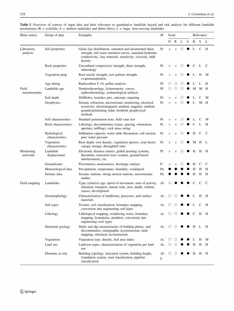
Table 3 Overview of sources of input data and their relevance to quantitative landslide hazard and risk analysis for different landslide

mechanisms (R = rockfalls, S = shallow landslides and debris flows, L = large, slow-moving landslides

Main source Group of data Examples M Scale Relevance

N R L S R S L

Laboratory

analysis

Soil properties Grain size distribution, saturated and unsaturated shear

strength, soil water retention curves, saturated hydraulic

conductivity, clay minerals, sensitivity, viscosity, bulk

density

Ps 9 9 s d L C H

Rock properties Unconfined compressive strength, shear strength,

mineralogy

Ps 9 9 s d C L C

Vegetation prop Root tensile strength, root pullout strength,

evapotranspiration

Ps 9 9 s d L H M

Age dating Radiocarbon C-14, pollen analysis Pf s s s d L L H

Field

measurements

Landslide age Dendrochronology, lichenometry, varves,

tephrochronology, archaeological artifacts

Pf s s s d M M H

Soil depth Drillholes, trenches, pits, outcrops, auguring Ps 9 9 s d L C M

Geophysics Seismic refraction, microseismic monitoring, electrical

resistivity, electromagnetic method, magnetic method,

ground-penetrating radar, borehole geophysical

methods

Ps 9 9 s d L M H

Soil characteristics Standard penetration tests, field vane test Ps 9 9 s d L C M

Rock characteristics Lithology, discontinuities (types, spacing, orientation,

aperture, infilling), rock mass rating

Ps 9 9 s d C L H

Hydrological

characteristics

Infiltration capacity, water table fluctuation, soil suction,

pore water pressure

Ps 9 9 s d H C C

Vegetation

characteristics

Root depth, root density, vegetation species, crop factor,

canopy storage, throughfall ratio

Ps 9 9 s d M H L

Monitoring

networks

Landslide

displacement

Electronic distance meters, global positing systems,

theodolite, terrestrial laser scanner, ground-based

interferometry, etc.

Pf 9 9 s d H H H

Groundwater Piezometers, tensiometers, discharge stations P 9 9 s d H C C

Meteorological data Precipitation, temperature, humidity, windspeed Pn d d d d H H H

Seismic data Seismic stations, strong motion stations, microseismic

studies

Pn d d d d H H H

Field mapping Landslides Type, (relative) age, speed of movement, state of activity,

initiation, transport, runout zone, area, depth, volume,

causes, development

Af s d d d C C C

Geomorphology Characterisation of landforms, processes, and surface

materials

Ac s s d d L H H

Soil types Texture, soil classification, boundary mapping,

conversion into engineering soil types

Ac s s d d L C H

Lithology Lithological mapping, weathering zones, boundary

mapping, formations, members, conversion into

engineering rock types

Ac s s d d C H H

Structural geology Strike and dip measurements of bedding planes, and

discontinuities, stratigraphic reconstruction, fault

mapping, structural reconstruction

Ac s s d d H L H

Vegetation Vegetation type, density, leaf area index Ac s s d d L H M

Land use Land-use types, characterisation of vegetation per land

use

Ac s s d d H H H

Elements at risk Building typology, structural system, building height,

foundation system, road classification, pipeline

classification

Af

L

s s d d H H H


123

as possible in both space and time, and which follows

international nomenclature (IAEG Commission on Land-

slides 1990).

Landslide inventories can be carried out using a variety

of techniques. A recent overview of the methods used for

landslide inventory mapping is given by Guzzetti et al.

(2012). Visual interpretation of stereoscopic imagery

(either aerial photographs or very high resolution optical

satellite images) remains the most widely used method, and

results in inventories of high resolution (Cardinali 2002)

when specific local conditions (such as vegetation limita-

tions) are met and when it is carried out by expert inter-

preters. Nowadays, the use of Google Earth data is a good

alternative for many areas, and many parts of the world are

covered by high-resolution imagery which can be down-

loaded and combined in GIS with a digital elevation model

to generate stereoscopic images, which are essential in

landslide interpretation. One of the most important devel-

opments is the use of shaded relief images produced from

LiDAR DEMs, from which the objects (e.g. vegetation) on

the Earth’s surface have been removed, for the visual

interpretation of landslide phenomena (Haugerud et al.

2003; Ardizzone et al. 2007; Van Den Eeckhaut et al. 2009;

Razak et al. 2011).

Landslide inventory mapping using visual stereo image

interpretation is a time-consuming task, and requires

extensive skills, training and perseverance. In many cases,

such skilled interpreters are not available, or landslide

inventories have to be produced within a short period of

time after the occurrence of a triggering event, requiring

the application of automated detection methods based on

remote sensing. Michoud et al. (2010) and Stumpf et al.

(2011) provide complete overviews of the various remote

sensing methods and tools that can be used for (semi-)

automated landslide mapping and monitoring. A large

number of methods make use of passive optical remote

sensing tools, such as pixel-based classification of or

change detection from spaceborne images (Hervas et al.

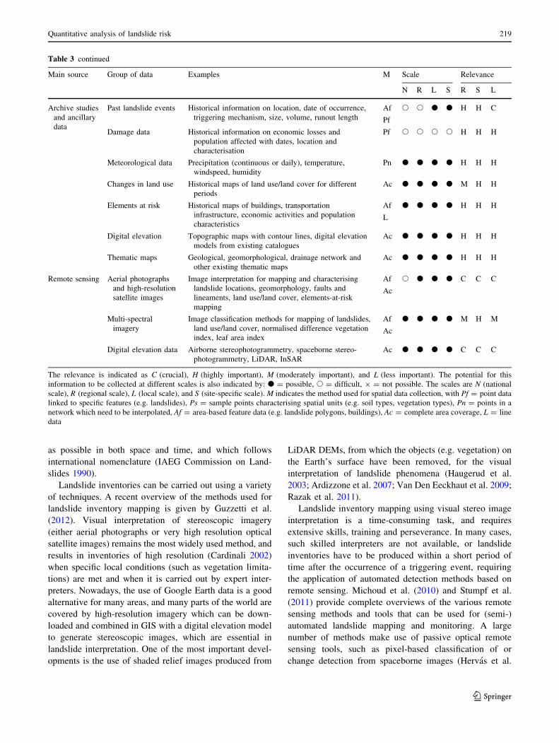
Table 3 continued

Main source Group of data Examples M Scale Relevance

N R L S R S L

Archive studies

and ancillary

data

Past landslide events Historical information on location, date of occurrence,

triggering mechanism, size, volume, runout length

Af

Pf

s s d d H H C

Damage data Historical information on economic losses and

population affected with dates, location and

characterisation

Pf s s s s H H H

Meteorological data Precipitation (continuous or daily), temperature,

windspeed, humidity

Pn d d d d H H H

Changes in land use Historical maps of land use/land cover for different

periods

Ac d d d d M H H

Elements at risk Historical maps of buildings, transportation

infrastructure, economic activities and population

characteristics

Af

L

d d d d H H H

Digital elevation Topographic maps with contour lines, digital elevation

models from existing catalogues

Ac d d d d H H H

Thematic maps Geological, geomorphological, drainage network and

other existing thematic maps

Ac d d d d H H H

Remote sensing Aerial photographs

and high-resolution

satellite images

Image interpretation for mapping and characterising

landslide locations, geomorphology, faults and

lineaments, land use/land cover, elements-at-risk

mapping

Af

Ac

s d d d C C C

Multi-spectral

imagery

Image classification methods for mapping of landslides,

land use/land cover, normalised difference vegetation

index, leaf area index

Af

Ac

d d d d M H M

Digital elevation data Airborne stereophotogrammetry, spaceborne stereo-

photogrammetry, LiDAR, InSAR

Ac d d d d C C C

The relevance is indicated as C (crucial), H (highly important), M (moderately important), and L (less important). The potential for this

information to be collected at different scales is also indicated by: d = possible, s = difficult, 9 = not possible. The scales are N (national

scale), R (regional scale), L (local scale), and S (site-specific scale). M indicates the method used for spatial data collection, with Pf = point data

linked to specific features (e.g. landslides), Ps = sample points characterising spatial units (e.g. soil types, vegetation types), Pn = points in a

network which need to be interpolated, Af = area-based feature data (e.g. landslide polygons, buildings), Ac = complete area coverage, L = line

data


123

2003; Borghuis et al. 2007; Mondini et al. 2011), or object-

oriented classification of or change detection from space-

borne images (Martha et al. 2010a; Lu et al. 2011).

Many methods used for landslide mapping and moni-

toring make use of digital elevation measurements that may

be derived from a wide range of tools, such as terrestrial

photographs (Travelletti et al. 2010), terrestrial videos,

UAV-based aerial photographs (Niethammer et al. 2011),

airborne stereophotogrammetry and spaceborne stereo-

photogrammetry (Martha et al. 2010b). Also, the applica-

tion of LiDAR data from both airborne laser scanning

(ALS) and terrestrial laser scanning (TLS) has proven very

successful (Jaboyedoff et al. 2012). Apart from LiDAR, the

most useful tool for landslide inventory mapping and

monitoring using remote sensing is in the InSAR domain.

Interferometric synthetic aperture radar (InSAR) has been

used extensively for measuring surface displacements.

Multi-temporal InSAR analyses using techniques such as

persistent scatterer (PS) InSAR (Ferretti et al. 2001) and

small baseline (SB) InSAR (Berardino et al. 2002) can be

used to measure the displacements of permanent scatterers

such as buildings with millimetre accuracy, and allow the

deformation history to be reconstructed (Farina et al.

2006).

Predisposing factors

Since topographic information and its various derivatives

play an important role in landslide hazard analysis, the use

of high-resolution digital elevation models (DEMs) is

crucial. DEMs can be derived through a large variety of

techniques, such as by digitising contours from existing

topographic maps, topographic levelling, electronic dis-

tance measurement (EDM), differential GPS measure-

ments, (digital) photogrammetry using imagery taken from

the ground or a wide range of platforms, InSAR, and

LiDAR. Global DEMs are now available from several

sources, such as the SRTM (Shuttle Radar Topography

Mission: Farr et al. 2007) and the ASTER (Advanced

Spaceborne Thermal Emission and Reflection Radiometer:

METI/NASA 2009). In the near future, a more accurate

global DEM is expected from TanDEM-X (TerraSAR-X

Add-On for Digital Elevation Measurements), which will

provide a DEM for the entire Earth’s surface to a vertical

accuracy of \2 m and a spatial accuracy of 12 m (Nelson

et al. 2009; Smith and Pain 2009). Many types of maps

(such as those of slope steepness, orientation, length, cur-

vature, upslope contributing area) can be derived from

DEMs using GIS operations.

Traditionally, geological maps represent a standard

component in heuristic and statistical landslide hazard

assessment methods (Aleotti and Chowdhury 1999; Dai

et al. 2002; Chacon et al. 2006). It is recommended that the

traditional legend of a geological map, which focuses on

the litho-stratigraphical subdivision into formations, should

be converted into an engineering geological classification

with more emphasis on Quaternary sediments and more

information on the rock composition and rock mass

strength. In detailed hazard studies, specific engineering

geological maps are generated and rock types are charac-

terised using field tests and laboratory measurements

(Dobbs et al. 2012). 3-D geological maps have been used

for detailed analyses, although the amount of outcrop and

borehole information collected limits this method to scales

of 1:5,000 or larger. Its use is generally restricted to the site

investigation level (e.g. Xie et al. 2003) at present,

although this may be expected to change in the future when

more detailed information becomes available from bore-

holes and geophysical studies, as computer technology and

data availability has transformed our ability to construct 3D

digital models of the shallow subsurface (e.g. Culshaw

2005).

Aside from lithological information, structural infor-

mation is very important for landslide hazard assessments.

At the medium and large scales, attempts have been made

to generate maps indicating dip direction and dip angle that

are based on field measurements, but the success of this

depends very strongly upon the number of structural

measurements and the complexity of the geological struc-

ture (Ghosh et al. 2010).

Representation of soil properties is a key problem in the

use of physically based slope stability models for landslide

hazard assessments, particularly for shallow failures such

as debris avalanches and debris slides, as well as deep-

seated slumps in soil (Guimaraes et al. 2003). Regolith

depth, often referred to by geomorphologists and engineers

as soil depth, is defined as the depth from the surface to

more-or-less consolidated material. Despite being a major

factor in landslide modelling, most studies have ignored its

spatial variability by using constant values over generalised

land units in their analyses (Bakker et al. 2005; Bathurst

et al. 2007; Talebi et al. 2008; Montgomery and Dietrich

1994; Santacana et al. 2003). Soil thickness can be mod-

elled using physically based methods that model rates of

weathering, denudation and accumulation (Dietrich et al.

1995; D’Odorico 2000) or empirical methods that deter-

mine correlations with topographical factors such as slope,

or it can be predicted using geostatistical methods (Tsai

et al. 2001; Van Beek 2002; Penızek and Boruvka 2006;

Catani et al. 2007). Such methods have also been used to

model the distributions of relevant geotechnical and

hydrological properties of soils (Hengl et al. 2004). How-

ever, the accurate modeling of soil thickness and parame-

ters over large areas remains difficult due to high spatial

variability. This implies that the final prediction of slope

hydrology and stability will still have a large component of


123

randomness. In addition to the limitations on accurately

determining the spatial variability, the measurement accu-

racy and the temporal variability of the parameters are two

other significant sources of error which will propagate into

the final simulation of slope hydrology and stability (Ku-

riakose et al. 2009).

Soil samples collected at different depths with the dril-

ling of boreholes and analysis of the grain-size distribution

curves provide additional information about soil depth and

bedrock topography, which is also important for deter-

mining subsurface hydrology.

Geomorphological maps are generated at various scales

to show land units based on their shapes, materials, pro-

cesses and genesis. Although some countries, such as

Germany, the Netherlands, Poland and Belgium, have

established legend systems to this end (Gustavsson et al.

2006), there is no generally accepted legend for geomor-

phological maps, and there may be large variations in

content based on the experience of the geomorphologist.

An important field within geomorphology is the quantita-

tive analysis of terrain forms from DEMs—called geo-

morphometry or digital terrain analysis. This combines

elements from the earth sciences, engineering, mathemat-

ics, statistics and computer science (Pike 2000). Part of the

work focuses on the automatic classification of geomor-

phological land units based on morphometric characteris-

tics at small scales (Asselen and Seijmonsbergen 2006), or

on the extraction of slope facets at medium scales which

can be used as the basic mapping units in statistical ana-

lysis (Cardinali 2002).

Land use is often considered a static factor in landslide

hazard studies, and relatively few studies have considered

changing land use as a factor in the analysis (Matthews

et al. 1997; Van Beek and Van Asch 2004). However, there

are an increasing number of studies that have analysed the

effect of land-use changes in landslide susceptibility

assessment (Glade 2003). For physically based modelling,

it is very important to have temporal land-use/land-cover

maps and to find the changes in the mechanical and

hydrological effects of vegetation. Land-use maps are

made on a routine basis from medium-resolution satellite

imagery. Although change detection techniques such as

post-classification comparison, temporal image differenc-

ing, temporal image ratioing, or Bayesian probabilistic

methods have been widely applied in land-use applications,

only fairly limited work has been done on the inclusion of

multi-temporal land-use change maps in landslide hazard

studies (Kuriakose 2010).

Triggering factors

Data relating to triggering factors represent another

important set of input data for landslide hazard assessment.

Data on precipitation, seismicity and anthropogenic activ-

ities have very important temporal components, knowledge

of which is required in the conversion of landslide sus-

ceptibility maps to hazard maps. The magnitude–frequency

relation for the triggering event is used to determine the

probability of landslide occurrences caused by that partic-

ular trigger. Magnitude–frequency relations of triggering

events can be linked to landslide occurrence in several

ways, as will be discussed in the ‘‘Derivation of M–F

relations’’ section. Rainfall and temperature data are col-

lected at meteorological stations, and values throughout the

study area are then derived through interpolation of the

station data. After that, correlations between precipitation

indicators and dates of historical landslide occurrences are

elucidated in order to establish rainfall thresholds (Cepeda

et al. 2012). A good example in Europe is the European

Climate Assessment & Dataset project (http://eca.knmi.nl/).

The use of weather radar for rainfall prediction in landslide

studies is a promising approach, as it allows storm cells to

be tracked with high spatial resolution, which in turn per-

mits short-term forecasts or warnings (e.g. Crosta and

Frattini 2003).

Physically based models for landslide susceptibility can

incorporate rainfall as a dynamic input of the model, which

allows susceptibility maps for future scenarios with cli-

matic change to be prepared (Collison et al. 2000; Mel-

chiorre and Frattini 2012; Comegna et al. 2012). Analysis

of earthquake-triggered landslide susceptibility and hazard

is still not very well developed due to the difficulty

involved in determining possible earthquake scenarios, for

example with respect to the antecedent moisture conditions

and their associated co-seismic landslide distributions

(Keefer 2002; Meunier et al. 2007; Gorum et al. 2011). In

order to establish better relationships between seismic,

geological and terrain factors for the prediction of co-

seismic landslide distributions, more digital event-based

co-seismic landslide inventories need to be produced for

different environments, earthquake magnitudes and fault-

ing mechanisms. Another approach to earthquake-induced

landslide susceptibility mapping uses a heuristic rule-based

approach in GIS with factor maps related to shaking

intensity (using the USGS ShakeMap data), slope angle,

material type, moisture, slope height and terrain roughness

(Miles and Keefer 2009).

Elements at risk

Elements at risk are all of the elements that may be affected

by the occurrence of hazardous phenomena, such as pop-

ulation, property or the environment. The consequences of

a landslide and subsequently the risk depend on the type of

elements that are present in an area. Inventories of ele-

ments at risk can be carried out at various levels, depending


123

http://eca.knmi.nl/

on the objectives of the study (Alexander 2005). Elements-

at-risk data should be collected for certain basic spatial

units, which may be grid cells, administrative units or

homogeneous units with similar characteristics in terms of

type and density of elements at risk. Risk can also be

analysed for linear features (e.g. transportation lines) and

specific sites (e.g. a dam site).

Building information can be obtained in several ways.

Ideally, it is available as building footprint maps, with

associated attribute information on building typology,

structural system, building height, foundation type, as well

as the value of the building and its contents (Pitilakis et al.

2011). It can also be derived from existing cadastral dat-

abases and (urban) planning maps, or it may be available in

an aggregated form as the number and types of buildings

per administrative unit. If such data are not available,

building footprint maps can be generated using screen

digitisation from high-resolution images, or through auto-

mated building mapping using high-resolution multispec-

tral satellite images and LiDAR (Brenner 2005).

Population data sets have static and dynamic compo-

nents. The static component relates to the number of

inhabitants per mapping unit and their characteristics,

whereas the dynamic component refers to their activity

patterns and their distribution in space and time. Population

distributions can be expressed in terms of either the abso-

lute number of people per mapping unit or the population

density. Census data are the obvious source of demo-

graphic data. However, for many areas, census data are

unavailable, outdated or unreliable. Therefore, other

approaches may also be used to model the population

distribution along with remote sensing and GIS, in order to

refine the spatial resolution of population data from avail-

able population information (so-called dasymetric map-

ping, Chen et al. 2004).

Data quality

The occurrence of landslides is governed by complex

interrelationships between factors, some of which cannot

be determined in detail, and others only with a large degree

of uncertainty. Some important aspects in this respect are

the error, accuracy, uncertainty and precision of the input

data, and the objectivity and reproducibility of the input

maps (see the ‘‘Evaluation of the performance of landslide

zonation maps’’ section). The accuracy of input data refers

to the degree of closeness of the measured or mapped

values or classes of a map to its actual (true) value or class

in the field. An error is defined as the difference between

the mapped value or class and the true one. The precision

of a measurement is the degree to which repeated mea-

surements under unchanged conditions show the same

results. Uncertainty refers to the degree to which the actual

characteristics of the terrain can be represented spatially in

a map.

The error in a map can only be assessed if another map

or other field information is available that is error-free and

can be used for verification (e.g. elevation). DEM error

sources have been described by Heuvelink (1998) and Pike

(2000); these can be related to the age of data, incomplete

density of observations or spatial sampling, processing

errors such as numerical errors in the computer, interpo-

lation errors or classification and generalisation problems

and measurement errors such as positional inaccuracy (in

the x- and y-directions), data entry faults, or observer bias.

Reviews of the uncertainties associated with digital ele-

vation models are provided by Fisher and Tate (2006),

Wechsler (2007) and Smith and Pain (2009). The quality of

the input data used for landslide hazard and risk analysis is

related to many factors, such as the scale of the analysis,

the time and money allocated for data collection, the size of

the study area, the experience of the researchers, and the

availability and reliability of existing maps. Also, existing

landslide databases often present several drawbacks (Ar-

dizzone et al. 2002; Van Den Eeckhaut and Hervas 2012)

related to their spatial and (especially) temporal com-

pleteness (or incompleteness), and the fact that they are

biased toward landslides that have affected infrastructure

such as roads.

Suggested methods for landslide susceptibility

assessment

A landslide susceptibility map subdivides the terrain into

zones with differing likelihoods that landslides of a certain

type may occur. Landslide susceptibility assessment can be

considered the initial step towards a landslide hazard and

risk assessment, but it can also be an end product in itself

that can be used in land-use planning and environmental

impact assessment. This is especially the case in small-

scale analyses or in situations where insufficient informa-

tion is available on past landslide occurrence to allow the

spatial and temporal probabilities of events to be assessed.

Landslide susceptibility maps contain information on

the type of landslides that might occur and on their spatial

likelihood of occurrence in terms of identifying the most

probable initiation areas (based on a combination of geo-

logical, topographical and land-cover conditions) and the

possibility of extension (upslope through retrogression and/

or downslope through runout). The likelihood may be

indicated quantitatively through indicators (such as the

density as the number per square kilometre, or the area

affected per square kilometre).

The methods used for landslide susceptibility analysis

are usually based on two assumptions. The first is that past


123

conditions are indicative of future conditions. Therefore,

areas that have experienced landslides in the past are likely

to experience them in the future too, as they maintain

similar environmental settings (e.g. topography, geology,

soil, geomorphology and land use).

• Methods used for landslide susceptibility analysis are

usually based on the assumption that terrain units that

have similar environmental settings (e.g. topography,

lithology, engineering soils, geomorphology and land

use) and were affected by landslides in the past are

likely to experience landslides in the future. This

approach emphasises the need to collect detailed

landslide inventories before conducting any landslide

susceptibility assessment.

• In terms of visualisation, landslide susceptibility maps

should include

• Zones with different classes of susceptibility to

landslide initiation and runout for particular land-

slide types; for the purpose of clarity, the number of

classes should be limited to less than five

• An inventory of historic landslides, which allows

the user to compare the susceptibility classes with

actual historic landslides

• A legend with an explanation of the susceptibility

classes, including information on expected landslide

densities

As landslide susceptibility maps primarily provide a

proposed ranking of terrain units in terms of spatial prob-

ability of occurrence, they do not explicitly convey infor-

mation on landslide return periods.

Landslide susceptibility assessment

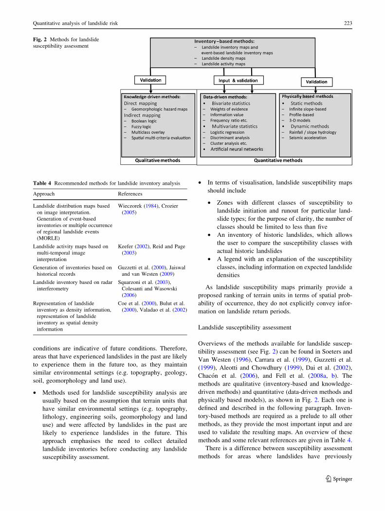
Overviews of the methods available for landslide suscep-

tibility assessment (see Fig. 2) can be found in Soeters and

Van Westen (1996), Carrara et al. (1999), Guzzetti et al.

(1999), Aleotti and Chowdhury (1999), Dai et al. (2002),

Chacon et al. (2006), and Fell et al. (2008a, b). The

methods are qualitative (inventory-based and knowledge-

driven methods) and quantitative (data-driven methods and

physically based models), as shown in Fig. 2. Each one is

defined and described in the following paragraph. Inven-

tory-based methods are required as a prelude to all other

methods, as they provide the most important input and are

used to validate the resulting maps. An overview of these

methods and some relevant references are given in Table 4.

There is a difference between susceptibility assessment

methods for areas where landslides have previously

Table 4 Recommended methods for landslide inventory analysis

Approach References

Landslide distribution maps based

on image interpretation.

Generation of event-based

inventories or multiple occurrence

of regional landslide events

(MORLE)

Wieczorek (1984), Crozier

(2005)

Landslide activity maps based on

multi-temporal image

interpretation

Keefer (2002), Reid and Page

(2003)

Generation of inventories based on

historical records

Guzzetti et al. (2000), Jaiswal

and van Westen (2009)

Landslide inventory based on radar

interferometry

Squarzoni et al. (2003),

Colesanti and Wasowski

(2006)

Representation of landslide

inventory as density information,

representation of landslide

inventory as spatial density

information

Coe et al. (2000), Bulut et al.

(2000), Valadao et al. (2002)

Fig. 2 Methods for landslide

susceptibility assessment


123

occurred and susceptibility assessment methods for areas

where landslides might occur but no landslide has occurred

previously. It should be noted that there is a direct relation

between the scale of the zoning map and the complexity of

the landslide susceptibility assessment method, with more

complex methods being applied at larger scales due to the

increased amount of data required. In knowledge-driven or

heuristic methods, the landslide susceptibility map can be

prepared directly in the field by expert geomorphologists,

or created in the office as a derivative map of a geomor-

phological map. The method is direct, as the expert inter-

prets the susceptibility of the terrain directly in the field,

based on the observed phenomena and the geomorpholo-

gical/geological setting. In the direct method, GIS is used

as a tool for entering the final map without extensive

modelling. Knowledge-driven methods can also be applied

indirectly using a GIS, by combining a number of factor

maps that are considered to be important for landslide

occurrence. On the basis of his/her expert knowledge on

past landslide occurrences and their causal factors within a

given area, an expert assigns particular weights to certain

combinations of factors. In knowledge-driven methods,

susceptibility is expressed in a qualitative form. In the

following, only quantitative methods are discussed.

Data-driven landslide susceptibility assessment methods

In data-driven landslide susceptibility assessment methods,

the combinations of factors that have triggered landslides

in the past are evaluated statistically, and quantitative

predictions are made for current non-landslide-affected

areas with similar geological, topographical and land-cover

conditions. No information on the historicity of the terrain

units in relation to multiple landslide events is considered.

The output may be expressed in terms of probability.

These methods are termed ‘‘data-driven’’, as data from past

landslide occurrences are used to obtain information on the

relative importances of the factor maps and classes. Three

main data-driven approaches are commonly used: bivari-

ate, multivariate and active learning statistical analysis

(Table 5). In bivariate statistical methods, each factor map

is combined with the landslide distribution map, and

weight values based on landslide densities are calculated

for each parameter class. Several statistical methods can be

applied to calculate weight values, such as the information

value method, weights of evidence modelling, Bayesian

combination rules, certainty factors, the Dempster–Shafer

method, and fuzzy logic. Bivariate statistical methods are a

good learning tool that the analyst can use to determine

which factors or combination of factors play a role in the

initiation of landslides. It does not take into account the

interdependence of variables, and it has to serve as a guide

when exploring the dataset before multivariate statistical

methods are used. Multivariate statistical models evaluate

the combined relationship between a dependent variable

(landslide occurrence) and a series of independent vari-

ables (landslide controlling factors). In this type of ana-

lysis, all relevant factors are sampled either on a grid basis

or in slope morphometric units. For each of the sampling

units, the presence or absence of landslides is determined.

The resulting matrix is then analysed using multiple

regression, logistic regression, discriminant analysis, ran-

dom forest or active learning. The results can be expressed

in terms of probability. Data-driven susceptibility methods

can be affected by shortcomings such as (a) the general

assumption that landslides occur due to the same combi-

nation of factors throughout a study area, (b) ignorance of

the fact that the occurrence of certain landslide types is

controlled by certain causal factors that should be analysed/

investigated individually, (c) the extent of control over

some spatial factors can vary widely in areas with complex

geological and structural settings, and (d) the lack of

suitable expert opinion on different landslide types, pro-

cesses and causal factors. These techniques have become

standard in regional scale landslide susceptibility

assessment.

Physically based landslide susceptibility assessment

methods

Physically based landslide susceptibility assessment

methods are based on the modelling of slope failure pro-

cesses. The methods are only applicable over large areas

when the geological and geomorphological conditions are

fairly homogeneous and the landslide types are simple

(Table 6). Most physically based models that are applied at

a local scale make use of the infinite slope model and are

Table 5 Recommended methods for data-driven landslide suscepti-

bility assessment

Method References

Bivariate

statistical

methods

Likelihood ratio

model (LRM)

Lee (2005)

Information

value method

Yin and Yan (1988)

Weights of

evidence

modelling

van Westen (1993), Bonham-

Carter (1994), Suzen and

Doyuran (2004)

Favourability

functions

Chung and Fabbri (1993), Luzi

(1995)

Multivariate

statistical

method

Discriminant

analysis

Carrara (1983), Gorsevski et al.

(2000)

Logistic

regression

Ohlmacher and Davis (2003),

Gorsevski et al. (2006a)

ANN Artificial neural

networks

Lee et al. (2004), Ermini et al.

(2005), Kanungo et al. (2006)


123

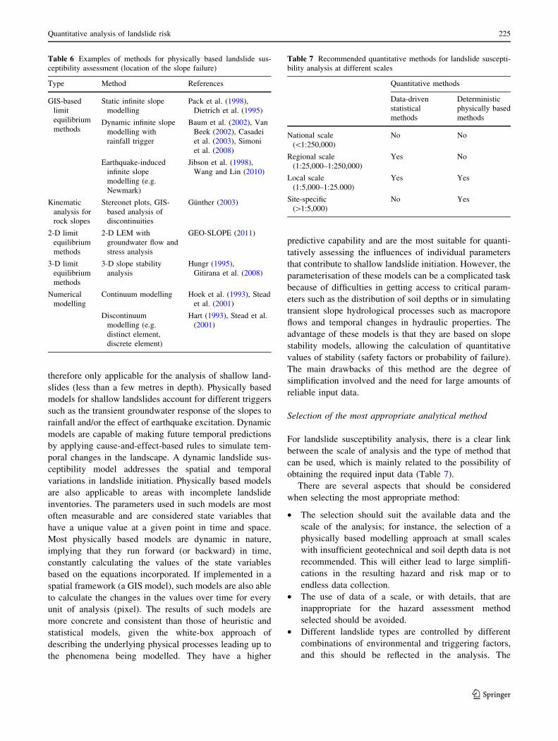
therefore only applicable for the analysis of shallow land-

slides (less than a few metres in depth). Physically based

models for shallow landslides account for different triggers

such as the transient groundwater response of the slopes to

rainfall and/or the effect of earthquake excitation. Dynamic

models are capable of making future temporal predictions

by applying cause-and-effect-based rules to simulate tem-

poral changes in the landscape. A dynamic landslide sus-

ceptibility model addresses the spatial and temporal

variations in landslide initiation. Physically based models

are also applicable to areas with incomplete landslide

inventories. The parameters used in such models are most

often measurable and are considered state variables that

have a unique value at a given point in time and space.

Most physically based models are dynamic in nature,

implying that they run forward (or backward) in time,

constantly calculating the values of the state variables

based on the equations incorporated. If implemented in a

spatial framework (a GIS model), such models are also able

to calculate the changes in the values over time for every

unit of analysis (pixel). The results of such models are

more concrete and consistent than those of heuristic and

statistical models, given the white-box approach of

describing the underlying physical processes leading up to

the phenomena being modelled. They have a higher

predictive capability and are the most suitable for quanti-

tatively assessing the influences of individual parameters

that contribute to shallow landslide initiation. However, the

parameterisation of these models can be a complicated task

because of difficulties in getting access to critical param-

eters such as the distribution of soil depths or in simulating

transient slope hydrological processes such as macropore

flows and temporal changes in hydraulic properties. The

advantage of these models is that they are based on slope

stability models, allowing the calculation of quantitative

values of stability (safety factors or probability of failure).

The main drawbacks of this method are the degree of

simplification involved and the need for large amounts of

reliable input data.

Selection of the most appropriate analytical method

For landslide susceptibility analysis, there is a clear link

between the scale of analysis and the type of method that

can be used, which is mainly related to the possibility of

obtaining the required input data (Table 7).

There are several aspects that should be considered

when selecting the most appropriate method:

• The selection should suit the available data and the

scale of the analysis; for instance, the selection of a

physically based modelling approach at small scales

with insufficient geotechnical and soil depth data is not

recommended. This will either lead to large simplifi-

cations in the resulting hazard and risk map or to

endless data collection.

• The use of data of a scale, or with details, that are

inappropriate for the hazard assessment method

selected should be avoided.

• Different landslide types are controlled by different

combinations of environmental and triggering factors,

and this should be reflected in the analysis. The

Table 6 Examples of methods for physically based landslide sus-

ceptibility assessment (location of the slope failure)

Type Method References

GIS-based

limit

equilibrium

methods

Static infinite slope

modelling

Pack et al. (1998),

Dietrich et al. (1995)

Dynamic infinite slope

modelling with

rainfall trigger

Baum et al. (2002), Van

Beek (2002), Casadei

et al. (2003), Simoni

et al. (2008)

Earthquake-induced

infinite slope

modelling (e.g.

Newmark)

Jibson et al. (1998),

Wang and Lin (2010)

Kinematic

analysis for

rock slopes

Stereonet plots, GIS-

based analysis of

discontinuities

Gunther (2003)

2-D limit

equilibrium

methods

2-D LEM with

groundwater flow and

stress analysis

GEO-SLOPE (2011)

3-D limit

equilibrium

methods

3-D slope stability

analysis

Hungr (1995),

Gitirana et al. (2008)

Numerical

modelling

Continuum modelling Hoek et al. (1993), Stead

et al. (2001)

Discontinuum

modelling (e.g.

distinct element,

discrete element)

Hart (1993), Stead et al.

(2001)

Table 7 Recommended quantitative methods for landslide suscepti-

bility analysis at different scales

Quantitative methods

Data-driven

statistical

methods

Deterministic

physically based

methods

National scale

(\1:250,000)

No No

Regional scale

(1:25,000–1:250,000)

Yes No

Local scale

(1:5,000–1:25.000)

Yes Yes

Site-specific

([1:5,000)

No Yes


123

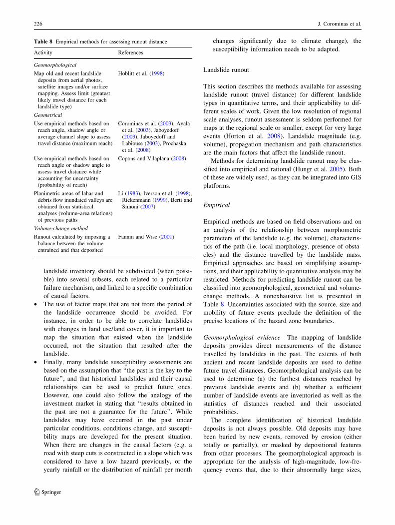
landslide inventory should be subdivided (when possi-

ble) into several subsets, each related to a particular

failure mechanism, and linked to a specific combination

of causal factors.

• The use of factor maps that are not from the period of

the landslide occurrence should be avoided. For

instance, in order to be able to correlate landslides

with changes in land use/land cover, it is important to

map the situation that existed when the landslide

occurred, not the situation that resulted after the

landslide.

• Finally, many landslide susceptibility assessments are

based on the assumption that ‘‘the past is the key to the

future’’, and that historical landslides and their causal

relationships can be used to predict future ones.

However, one could also follow the analogy of the

investment market in stating that ‘‘results obtained in

the past are not a guarantee for the future’’. While

landslides may have occurred in the past under

particular conditions, conditions change, and suscepti-

bility maps are developed for the present situation.

When there are changes in the causal factors (e.g. a

road with steep cuts is constructed in a slope which was

considered to have a low hazard previously, or the

yearly rainfall or the distribution of rainfall per month

changes significantly due to climate change), the

susceptibility information needs to be adapted.

Landslide runout

This section describes the methods available for assessing

landslide runout (travel distance) for different landslide

types in quantitative terms, and their applicability to dif-

ferent scales of work. Given the low resolution of regional

scale analyses, runout assessment is seldom performed for

maps at the regional scale or smaller, except for very large

events (Horton et al. 2008). Landslide magnitude (e.g.

volume), propagation mechanism and path characteristics

are the main factors that affect the landslide runout.

Methods for determining landslide runout may be clas-

sified into empirical and rational (Hungr et al. 2005). Both

of these are widely used, as they can be integrated into GIS

platforms.

Empirical

Empirical methods are based on field observations and on

an analysis of the relationship between morphometric

parameters of the landslide (e.g. the volume), characteris-

tics of the path (i.e. local morphology, presence of obsta-

cles) and the distance travelled by the landslide mass.

Empirical approaches are based on simplifying assump-

tions, and their applicability to quantitative analysis may be

restricted. Methods for predicting landslide runout can be

classified into geomorphological, geometrical and volume-

change methods. A nonexhaustive list is presented in

Table 8. Uncertainties associated with the source, size and

mobility of future events preclude the definition of the

precise locations of the hazard zone boundaries.

Geomorphological evidence The mapping of landslide

deposits provides direct measurements of the distance

travelled by landslides in the past. The extents of both

ancient and recent landslide deposits are used to define

future travel distances. Geomorphological analysis can be

used to determine (a) the farthest distances reached by

previous landslide events and (b) whether a sufficient

number of landslide events are inventoried as well as the

statistics of distances reached and their associated

probabilities.

The complete identification of historical landslide

deposits is not always possible. Old deposits may have

been buried by new events, removed by erosion (either

totally or partially), or masked by depositional features

from other processes. The geomorphological approach is

appropriate for the analysis of high-magnitude, low-fre-

quency events that, due to their abnormally large sizes,

Table 8 Empirical methods for assessing runout distance

Activity References

Geomorphological

Map old and recent landslide

deposits from aerial photos,

satellite images and/or surface

mapping. Assess limit (greatest

likely travel distance for each

landslide type)

Hoblitt et al. (1998)

Geometrical

Use empirical methods based on

reach angle, shadow angle or

average channel slope to assess

travel distance (maximum reach)

Corominas et al. (2003), Ayala

et al. (2003), Jaboyedoff

(2003), Jaboyedoff and

Labiouse (2003), Prochaska

et al. (2008)

Use empirical methods based on

reach angle or shadow angle to

assess travel distance while

accounting for uncertainty

(probability of reach)

Copons and Vilaplana (2008)

Planimetric areas of lahar and

debris flow inundated valleys are

obtained from statistical

analyses (volume–area relations)

of previous paths

Li (1983), Iverson et al. (1998),

Rickenmann (1999), Berti and

Simoni (2007)

Volume-change method

Runout calculated by imposing a

balance between the volume

entrained and that deposited

Fannin and Wise (2001)


123

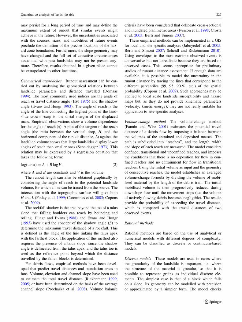
may persist for a long period of time and may define the

maximum extent of runout that similar events might

achieve in the future. However, the uncertainties associated

with the sources, sizes, and mobilities of future events

preclude the definition of the precise locations of the haz-

ard zone boundaries. Furthermore, the slope geometry may

have changed and the full set of causative circumstances

associated with past landslides may not be present any-

more. Therefore, results obtained in a given place cannot

be extrapolated to other locations.

Geometrical approaches Runout assessment can be car-

ried out by analysing the geometrical relations between

landslide parameters and distance travelled (Domaas

1994). The most commonly used indices are the angle of

reach or travel distance angle (Hsu 1975) and the shadow

angle (Evans and Hungr 1993). The angle of reach is the

angle of the line connecting the highest point of the land-

slide crown scarp to the distal margin of the displaced

mass. Empirical observations show a volume dependence

for the angle of reach (a). A plot of the tangent of the reach

angle (the ratio between the vertical drop, H, and the

horizontal component of the runout distance, L) against the

landslide volume shows that large landslides display lower

angles of reach than smaller ones (Scheidegger 1973). This

relation may be expressed by a regression equation that

takes the following form:

logðtan aÞ ¼ Aþ B log V; ð2Þ

where A and B are constants and V is the volume.

The runout length can also be obtained graphically by

considering the angle of reach to the potential landslide

volume, for which a line can be traced from the source. The

intersection with the topographic surface will give both

H and L (Finlay et al. 1999; Corominas et al. 2003; Copons

et al. 2009).

The rockfall shadow is the area beyond the toe of a talus

slope that falling boulders can reach by bouncing and

rolling. Hungr and Evans (1988) and Evans and Hungr

(1993) have used the concept of the shadow angle (b) to

determine the maximum travel distance of a rockfall. This

is defined as the angle of the line linking the talus apex

with the farthest block. The application of this method also

requires the presence of a talus slope, since the shadow

angle is delineated from the talus apex, and the talus toe is

used as the reference point beyond which the distance

travelled by the fallen blocks is determined.

For debris flows, empirical methods have been devel-

oped that predict travel distances and inundation areas in

fans. Volume, elevation and channel slope have been used

to estimate the total travel distance (Rickenmann 1999,

2005) or have been determined on the basis of the average

channel slope (Prochaska et al. 2008). Volume balance

criteria have been considered that delineate cross-sectional

and inundated planimetric areas (Iverson et al. 1998; Crosta

et al. 2003; Berti and Simoni 2007).

These empirical methods can be implemented in a GIS

for local and site-specific analyses (Jaboyedoff et al. 2005;

Berti and Simoni 2007; Scheidl and Rickenmann 2010).

Using envelopes to the most extreme observed events is

conservative but not unrealistic because they are based on

observed cases. This seems appropriate for preliminary

studies of runout distance assessment. If enough data are

available, it is possible to model the uncertainty in the

runout distance by tracing the lines that correspond to the

different percentiles (99, 95, 90 %, etc.) of the spatial

probability (Copons et al. 2009). Such approaches may be

applied to local scale landslide susceptibility and hazard

maps but, as they do not provide kinematic parameters

(velocity, kinetic energy), they are not really suitable for

application to site-specific analyses.

Volume-change method The volume-change method

(Fannin and Wise 2001) estimates the potential travel

distance of a debris flow by imposing a balance between

the volumes of the entrained and deposited masses. The

path is subdivided into ‘‘reaches’’, and the length, width

and slope of each reach are measured. The model considers

confined, transitional and unconfined reaches, and imposes

the conditions that there is no deposition for flow in con-

fined reaches and no entrainment for flow in transitional

reaches. Using the initial volume as input and the geometry

of consecutive reaches, the model establishes an averaged

volume-change formula by dividing the volume of mobi-

lised material by the length of the debris trail. The initial

mobilised volume is then progressively reduced during

downslope flow until the movement stops (i.e. the volume

of actively flowing debris becomes negligible). The results

provide the probability of exceeding the travel distance,

which is compared with the travel distances of two

observed events.

Rational methods

Rational methods are based on the use of analytical or

numerical models with different degrees of complexity.

They can be classified as discrete or continuum-based

models.

Discrete models These models are used in cases where

the granularity of the landslide is important, i.e. where

the structure of the material is granular, so that it is

possible to represent grains as individual discrete ele-

ments. The simplest case is that of a block which falls

on a slope. Its geometry can be modelled with precision

or approximated by a simpler form. The model checks


123

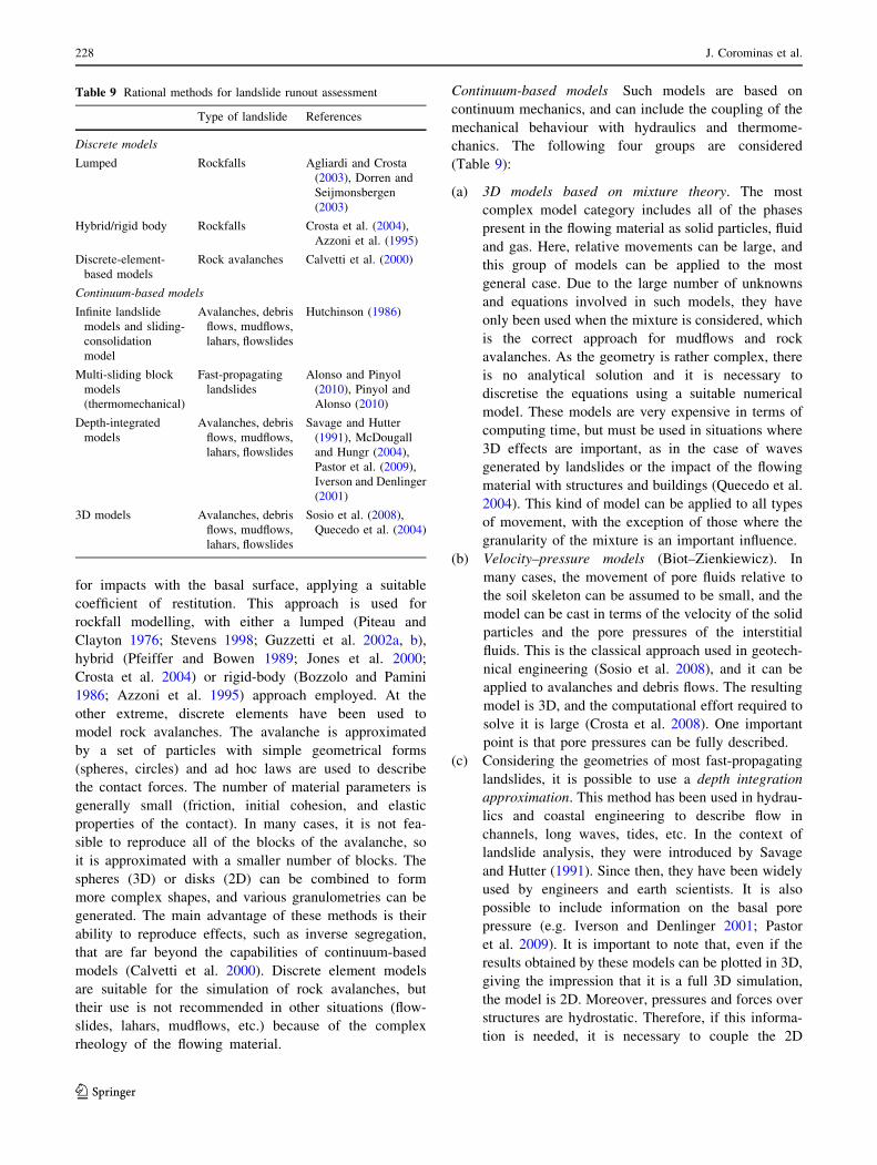
for impacts with the basal surface, applying a suitable

coefficient of restitution. This approach is used for

rockfall modelling, with either a lumped (Piteau and

Clayton 1976; Stevens 1998; Guzzetti et al. 2002a, b),

hybrid (Pfeiffer and Bowen 1989; Jones et al. 2000;

Crosta et al. 2004) or rigid-body (Bozzolo and Pamini

1986; Azzoni et al. 1995) approach employed. At the

other extreme, discrete elements have been used to

model rock avalanches. The avalanche is approximated

by a set of particles with simple geometrical forms

(spheres, circles) and ad hoc laws are used to describe

the contact forces. The number of material parameters is

generally small (friction, initial cohesion, and elastic

properties of the contact). In many cases, it is not fea-

sible to reproduce all of the blocks of the avalanche, so

it is approximated with a smaller number of blocks. The

spheres (3D) or disks (2D) can be combined to form

more complex shapes, and various granulometries can be

generated. The main advantage of these methods is their

ability to reproduce effects, such as inverse segregation,

that are far beyond the capabilities of continuum-based

models (Calvetti et al. 2000). Discrete element models

are suitable for the simulation of rock avalanches, but

their use is not recommended in other situations (flow-

slides, lahars, mudflows, etc.) because of the complex

rheology of the flowing material.

Continuum-based models Such models are based on

continuum mechanics, and can include the coupling of the

mechanical behaviour with hydraulics and thermome-

chanics. The following four groups are considered

(Table 9):

(a) 3D models based on mixture theory. The most

complex model category includes all of the phases

present in the flowing material as solid particles, fluid

and gas. Here, relative movements can be large, and

this group of models can be applied to the most

general case. Due to the large number of unknowns

and equations involved in such models, they have

only been used when the mixture is considered, which

is the correct approach for mudflows and rock

avalanches. As the geometry is rather complex, there

is no analytical solution and it is necessary to

discretise the equations using a suitable numerical

model. These models are very expensive in terms of

computing time, but must be used in situations where

3D effects are important, as in the case of waves

generated by landslides or the impact of the flowing

material with structures and buildings (Quecedo et al.

2004). This kind of model can be applied to all types

of movement, with the exception of those where the

granularity of the mixture is an important influence.

(b) Velocity–pressure models (Biot–Zienkiewicz). In

many cases, the movement of pore fluids relative to

the soil skeleton can be assumed to be small, and the

model can be cast in terms of the velocity of the solid

particles and the pore pressures of the interstitial

fluids. This is the classical approach used in geotech-

nical engineering (Sosio et al. 2008), and it can be

applied to avalanches and debris flows. The resulting

model is 3D, and the computational effort required to

solve it is large (Crosta et al. 2008). One important

point is that pore pressures can be fully described.

(c) Considering the geometries of most fast-propagating

landslides, it is possible to use a depth integration

approximation. This method has been used in hydrau-

lics and coastal engineering to describe flow in

channels, long waves, tides, etc. In the context of

landslide analysis, they were introduced by Savage

and Hutter (1991). Since then, they have been widely

used by engineers and earth scientists. It is also

possible to include information on the basal pore

pressure (e.g. Iverson and Denlinger 2001; Pastor

et al. 2009). It is important to note that, even if the

results obtained by these models can be plotted in 3D,

giving the impression that it is a full 3D simulation,

the model is 2D. Moreover, pressures and forces over

structures are hydrostatic. Therefore, if this informa-

tion is needed, it is necessary to couple the 2D

Table 9 Rational methods for landslide runout assessment

Type of landslide References

Discrete models

Lumped Rockfalls Agliardi and Crosta

(2003), Dorren and

Seijmonsbergen

(2003)

Hybrid/rigid body Rockfalls Crosta et al. (2004),

Azzoni et al. (1995)

Discrete-element-

based models

Rock avalanches Calvetti et al. (2000)

Continuum-based models

Infinite landslide

models and sliding-

consolidation

model

Avalanches, debris

flows, mudflows,

lahars, flowslides

Hutchinson (1986)

Multi-sliding block

models

(thermomechanical)

Fast-propagating

landslides

Alonso and Pinyol

(2010), Pinyol and

Alonso (2010)

Depth-integrated

models

Avalanches, debris

flows, mudflows,

lahars, flowslides

Savage and Hutter

(1991), McDougall

and Hungr (2004),

Pastor et al. (2009),

Iverson and Denlinger

(2001)

3D models Avalanches, debris

flows, mudflows,

lahars, flowslides

Sosio et al. (2008),

Quecedo et al. (2004)


123

depth-integrated model with the full 3D model in the

proximity of the obstacle. Depth-integrated models

represent an excellent compromise between computer

time and accuracy. They have been used to describe

rock avalanches, lahars, mudflows, debris flows and

flowslides (Agliardi and Crosta 2003; Hungr 1995;

McDougall and Hungr 2004; Pastor et al. 2002, 2009;

Quecedo et al. 2004; Savage and Hutter 1991; Sosio

et al. 2008, Laigle and Coussot 1997).

(d) Depth-integrated models can be simplified still

further, as in the case of so-called infinite landslide

approaches. Indeed, the block analysis performed in

many cases consists of a succession of infinite

landslides evolving over a variable topography. Pore

pressure dissipation can be included in such models

(e.g. Hutchinson 1986).

Landslide hazard assessment

Hazard assessment aims to determine the spatial and tem-

poral probability of occurrence of landslides in the target

area, along with their mode of propagation, size and

intensity. A complete analysis has to take into account all

of the possible failure mechanisms, the reactivation of

dormant landslides, and the acceleration of active ones. A

well-known definition of landslide hazard refers to the

probability of occurrence of a landslide of a given mag-

nitude (Varnes 1984). The magnitude is the measure of the

landslide size, which is usually expressed as either an area

or volume. However, the landslide magnitude is not an

appropriate hazard descriptor. Even though it may be

expected that the larger the landslide, the higher the

potential for damage, this does not hold true in all cases. A

large creeping landslide mobilizing hundreds of millions of

cubic metres at a rate of displacement of a few mm/year

would cause only slight damage to buildings or infra-

structure, and a negligible threat to people. In contrast, a

rockfall of a few hundreds of cubic metres travelling at tens

of m/s has the capacity to cause significant damage to

structures and loss of life.

Landslide destructiveness is best represented by its

intensity (Hungr 1997). Intensity is expressed differently

depending on the propagation mechanism. For landslides

that cause localised impacts, such as rockfalls, the velocity

of the event coupled with its volume or the kinetic energy

can be used. For slow-moving landslides, the differential

displacement or the total displacement (which may cause

damage or disturbance to structural elements) is used. The

depth of debris, the peak discharge per unit of width, or the

impact pressure can be used to characterise the intensities

of flow-like movements. Assessing landslide intensity is

not a straightforward task, because it is not an intrinsic

characteristic of the landslide. It changes along the path

and must be either measured or computed using dynamic

models that take the landslide volume as an input param-

eter. In areas affected by slow-moving landslides, magni-

tude has been used as a proxy for the landslide intensity

(Guzzetti et al. 2005). Although it is not conceptually

correct, it may be a practical way to decide between dif-

ferent land-use planning options.

Irrespective of the scale of work, hazard assessment

must specify a time frame for the occurrence of all

potential landslide types and their intensities at any con-

sidered location. This is the most difficult part of the

assessment because (a) different landslide types may occur

within different time frames, (b) the target area may be

affected by landslides originating from different source

areas, (c) the landslide frequency observed at any given

location or section will change with the distance from the

landslide source. Further discussion of these issues can be

found in the ‘‘Landslide hazard evaluation’’ section.

Temporal occurrence of landslides

The temporal occurrence of landslides is normally

expressed in terms of frequency, return period, or

exceedance probability. The frequency represents the

number of events in a certain time interval (e.g. annual

frequency), and it can conveniently be assessed from

empirical data. The return period is the inverse of the

annual probability, and refers to the average time interval

in which an event of a certain magnitude is expected to

occur. The exceedance can be considered the probability

that one or more events will occur in a certain period,

regardless of the magnitude of the events (Crovelli 2000).

Otherwise, if the magnitude of the events is accounted for,

the exceedance probability can be considered the proba-

bility that an event with a magnitude equal to or larger than

a certain value will occur in a certain period. The

exceedance probability is preferable as a measure of the

temporal occurrence of landslides for a quantitative prob-

abilistic hazard analysis, and can be derived from the fre-

quency (or return period) using an appropriate probabilistic

model, such as a binomial or Poisson model (Crovelli

2000) or a power-law distribution (Dussauge-Peisser et al.

2002).

Frequency may be absolute or relative (Corominas and

Moya 2008). Absolute frequency expresses the number of

observed events in a terrain unit (i.e. slope, debris fan,

watershed, etc.). It may consist of either the repeated

occurrence of first-time slope failures, reactivation events

of dormant landslides, or acceleration episodes (surges) of

active landslides. Rockfalls and debris flows are typical


123

landslide types treated as repetitive events. Relative fre-

quency is a normalised frequency. It is usually expressed as

the ratio of the number of observed landslide events to the

unit area or length (i.e. landslides/km2/year). The relative

frequency of landslides is appropriate when working with

large areas and/or at small scales, and particularly when

dealing with multiple-occurrence regional landslide events

or MORLE (Crozier 2005). Maps prepared at scales

smaller than 1:25,000 cannot effectively address the fre-

quency of individual small-sized landsides (up to a few

several thousands of cubic metres) because they are too

small to be mapped and treated individually.

The approaches traditionally followed to assess the

probability of occurrence of landslides are now described.

Heuristic methods (judgemental approach)

Heuristic methods are based on the expert judgements of a

group of specialists, whose opinions may be quantified by

assigning probabilities. One of the ways to systematise

heuristic evaluation is through event trees. An event tree

analysis is a graphical representation of all of the events

that can occur in a system. Using a logic model, the

probabilities of the possible outcomes following an initi-

ating event may be identified and quantified. As the num-

ber of possible outcomes increases, the figure spreads out

like the branches of a tree (Wong et al. 1997b). The

branching node probabilities have to be determined in

order to quantify the probabilities of the different alterna-

tives. The probability of a path giving a particular outcome,

such as a slope failure, is simply the product of the

respective branching node probabilities (Lee et al. 2000;

Budetta 2002; Wong 2005).

Rational methods (geomechanical approach)

The probability of slope failure may be determined by

means of stability analysis and numerical modelling. It is

important to point out that the outputs for these methods

can be implemented on GIS platforms and used to prepare

maps showing the potential for landslide occurrence from

hillslope source areas. However, they are not intended to

depict landslide paths or landslide deposition areas.

The geomechanical approach considers slope failure to

be dependent on space, time and stresses within the soil.

This allows the calculation of the factor of safety, or the

probability of failure. The latter is assumed to be the

probability of the factor of safety being less than unity.

Several methods have been developed to estimate this

probability, such as the first-order second moment (FOSM)

method, point estimate methods and Monte Carlo simula-

tions (Wu et al. 1996; Haneberg 2004; Wu and Abdel-Latif

2000). These methods take the uncertainties in the input

parameters into account. In order to assign a probability of

occurrence, it is necessary to explicitly couple the stability

analysis to a triggering factor with a known probability.

Slope stability may be coupled with hydrological models

to simulate the effect of rainfall on slope stability. For single

landslides at either the local or regional scale, transient

hydrogeological 2D or 3D finite-element or difference

models can be applied (Miller and Sias 1998; Tacher et al.

2005; Malet et al. 2005; Shrestha et al. 2008). For shallow

landslides, it is possible to implement regional scale analyses

by using simplified hydrological methods that can be

implemented in a spatially distributed GIS analysis (Mont-

gomery and Dietrich 1994; Pack et al. 1998; Iverson 2000;

Crosta and Frattini 2003; Baum et al. 2005; Godt et al. 2008).

Empirical probability

Probabilistic models may be developed based upon the

observed frequency of past landslide events. This approach

is implemented in a similar manner to the hydrological

analyses, and the annual probability of occurrence is

obtained. In this case, landslides are considered recurrent

events that occur randomly and independently. These

assumptions do not hold completely true for landslides,

particularly that the events are independent, and that

external (e.g. climatic) conditions are static. However, they

may be accepted as a first-order approach and, quite often,

frequency analysis is the only feasible method of estimat-

ing the temporal probability of occurrence of landslides.

The binomial or the Poisson distribution is typically

used to obtain the probability of landsliding (Crovelli

2000). The binomial distribution can be applied to the

cases in which discrete time intervals are considered and

only one observation is made per interval (usually per

year), as is typically the case in flood frequency analysis.

The annual probability of a landslide event of a given

magnitude which occurs on average once every T years is

P N ¼ 1; t ¼ 1ð Þ ¼ 1

T¼ k; ð3Þ

where T is the return period of the event and k is the

expected frequency of future occurrences.

The Poisson distribution arises as a limit case of the

binomial distribution when the increments of time are very

small (tending to 0), which is why the Poisson distribution is

said to be a continuous-time distribution. The annual prob-

ability of having n landslide events for a Poisson model is

P N ¼ n; t ¼ 1ð Þ ¼ ðktÞn

n!e�kt; ð4Þ

where k is the expected frequency of future landslides. On

the other hand, the probability of occurrence of one or

more landslides in t years is


123

P N� 1; tð Þ ¼ 1� e�kt; ð5Þ

which strongly depends on the magnitude of the landslide

events. Consequently, magnitude–frequency (M–F) rela-

tions should be established in order to carry out the

quantitative assessment of the landslide hazard. It must be

taken into account that different landslide types occur with

different temporal patterns. In the event that the same

location is potentially affected by the arrival of different

landslide types from different sources, an increase in the

probability of occurrence will result, and the combined

frequency must be calculated.

Indirect approaches

The definition of landslide-triggering rainfall and earth-

quake thresholds has been a topic of great interest in recent

decades. Plotting rainfall intensity versus rainfall duration

for observed landslide events allows the construction of

region-specific curves which identify precipitation inten-

sity-durations that cause shallow landslides and debris

flows (Guzzetti et al. 2007, 2008).

Once the critical rainfall (or the earthquake) magnitude

has been determined, the return period of the landslides is

assumed to be that of the critical trigger. These types of

relationships give an estimate of how often landslides

occur in the study area, but not which slopes will fail; nor

do they indicate the size of the failure. In this case, the

probability of occurrence of the landslide triggering rainfall

allows the calculation of the relative frequency of land-

slides (i.e. the number of landslides/km2/year), which is

useful for regional analyses of homogeneously sized

landslides (Reid and Page 2003).

Regional landslide triggering events might co-exist with

other regional triggers (e.g. snow melt), and with other

landslide triggers occurring at a local scale (e.g. river

erosion). In this case, the return period obtained from the

regional landslide trigger is only a minimum estimate of

the landslide frequency.

Magnitude–frequency relations

The landslide magnitude–frequency relation is the basis of

quantitative hazard assessment. Without a sound assess-

ment of the landslide occurrence probability, expressed in

terms of the expected annual frequency of landslide events

of a given magnitude, or exceeding a magnitude threshold,

a quantitative assessment of landslide hazard is not feasi-

ble. In this case, the problem can only be dealt with in

terms of susceptibility (e.g. spatial probability; Brabb

1984).

Specific relationships between the frequency of events

falling in different magnitude classes (i.e. magnitude–

frequency relationships) have been observed for different

natural hazards (e.g. earthquakes, floods). The first well-

established magnitude–frequency relationship was pro-

posed in seismology, where a relation between earthquake

magnitude and cumulative frequency was observed (the

Gutenberg–Richter equation), which is expressed as

logN mð Þ ¼ a� bM; ð6Þ

where N(m) is the cumulative number of earthquake events

with magnitudes equal or greater than M, and a and b are

constants.

The probability density function according to the

Gutenberg–Richter relation can be calculated as the

derivative of the corresponding cumulative density func-

tion. In practice, when simulating earthquakes, bounded

versions of the Gutenberg–Richter relation are used that

account for a lower cutoff for earthquake magnitude of

completeness as well as an expected upper one (Kramer

1996).

Early analyses of landslides (Hovius et al. 1997; Pelle-

tier et al. 1997) found that magnitude versus cumulative

frequency of the number of landslides is scale invariant and

that, for a wide range of landslide magnitudes, the relation

follows a power law which is formally equivalent to the

Gutenberg–Richter equation:

NCL ¼ CA�aL ; ð7Þ

where NCL is the cumulative number of landslide events

with magnitudes equal or greater than A, and AL is the

landslide magnitude (usually expressed as its size: volume

or area), while C and a are constants.

A similar distribution may be used for the noncumula-

tive distribution of landslides (Guzzeti et al. 2002b):

NL ¼ C0A�bL ; ð8Þ

where NL is the noncumulative number of landslide events

with magnitudes equal or greater than A, and AL is the

landslide magnitude (usually expressed as its size: volume

or area), while C0 and b are constants.

The construction and interpretation of frequency–mag-

nitude relations have been discussed by several researchers

(e.g. Guzzetti et al. 2002b; Brardinoni and Church 2004;

Malamud et al. 2004; Guthrie et al. 2008; Brunetti et al.

2009). Power laws can usually be adjusted to the frequency

distribution of events in a given magnitude class above a

particular magnitude threshold. Below this threshold, a

characteristic ‘‘rollover’’ effect may occur, resulting in a

deviation from the power law and an unrealistic underes-

timation of smaller events. While some researchers con-

sider that the rollover effect is usually not observed in

complete inventories, and that flattening of the magnitude–

frequency curves towards small magnitude values is related

to censoring effects (Hungr et al. 1999; Stark and Hovius


123

2001; Malamud et al. 2004), others consider that rollover is

the result of actual physiographic limitations (Pelletier

et al. 1997; Guthrie et al. 2008) or the effect of cohesion

(Van Den Eeckhaut et al. 2007).

Derivation of M–F relations

Different approaches may be followed depending on

whether M–F relations have been derived at a regional

scale or at particular locations. Lists of possible works on

how to prepare M–F relationships using different approa-

ches or different datasets are given in Tables 10 and 11.

Landslide magnitude may be expressed in terms of either

MORLE or individual landslide size.

In regional scale analyses, a relation may be estab-

lished between the intensity of the trigger (accumulated

rainfall, rainfall intensity, earthquake magnitude) and the

magnitude of the MORLE, which is given by either the

total number of landslides or, preferably, by landslide

areal density (i.e. number of landslides/km2) (Frattini

et al. 2009). Such a relation has been obtained in some

documented cases for storms (Reid and Page 2003) and

earthquakes (Keefer 2002). M–F relations can also be

prepared from the analysis of aerial photographs or

satellite images obtained at known time intervals. These

M–F relations may be valid at a regional level, but not

for any particular slope or subregion. It is important to

note that, in the aforementioned regional approaches,

landslide runout is not considered in the analyses

(Table 10).

In local scale analysis, the F–M relation calculated at the

source area can be significantly different from that calcu-

lated further downhill, as the volume of the landslide

influences the travel distance and the area covered by the

deposit. Consequently, the landslide frequency at any ter-

rain unit is due to both the occurrence of a slope failure and

the probability of being affected by landslides from

neighbouring areas.

The probability that a given slope unit is affected by

a landslide thus depends on the frequency of initiation,

which must be scaled according to the frequency of

reach, which in turn depends on the landslide dynam-

ics, as simulated by suitable models (Crosta and Ag-

liardi 2003). For hazard zoning purposes, such scaling

may be regarded as negligible for short-runout land-

slides, and hazard can be evaluated with respect to the

Table 10 Activities required to prepare non-spatially explicit mag-

nitude–frequency relations for landslides

Methodologies and data sources References

Occurrence of multiple-landslide-triggering events

Landslide density is related to the

intensity of the landslide-

triggering storm

Reid and Page (2003)

Landslide density (magnitude) is

related to the intensity of the

landslide-triggering earthquake

Keefer (2002)

Factor relating safety to rainfall or

piezometric level

Salciarini et al. (2008)

Cumulative occurrence of landslides over known time intervals

Analysis of landside records and

historical archives

Jaiswal and Van Westen (2009)

Identification and inventory of

landslides from aerial

photographs or satellite images

Hungr et al. (1999), Guthrie and

Evans (2004)

Landslide series completed by

dating landslide deposits and

field work

Schuster et al. (1992), Bull et al.

(1994), Bull and Brandon

(1998)

Landslide series completed using

proxy data such as silent

witnesses (e.g. tree damage)

Van Steijn (1996)

Table 11 Activities required to prepare spatially explicit magnitude–

frequency relations for landslides

Methodologies and data sources References

Source area

Landslide reactivation event

series prepared by dating the

associated landslide

reactivation features

Agliardi et al. (2009a)

Sizes of landslide scars Pelletier et al. (1997)

Probabilistic analysis of cliff

recession rates

Lee et al. (2002)

Reference section or location

Incident databases of roads and

railway maintenance teams

Bunce et al. (1997), Hungr et al.

(1999), Chau et al. (2003)

Spatial probability of occurrence

combined with the expected

probability of occurrence at

each slope

Guzzetti et al. (2005)

Landslide series completed using

proxy data such as silent

witnesses (e.g. tree damage)

Jakob and Friele (2010), Stoffel

(2010), Corominas and Moya

(2010), Lopez Saez et al.

(2012)

Landslide series completed by

dating landslide deposits and

field work

Van Dine et al. (2005), Jakob

(1996, 2012)

Integrated approach

Landslide frequency at the source

area combined with runout

models to obtain frequencies of

different landslide magnitudes

at a given control section

Corominas et al. (2005)

Landslide frequency at the source

area combined with runout

models to obtain spatial

distributions of different

landslide magnitudes

Agliardi et al. (2009b)


123

landslide source. Conversely, when coping with long-

runout landslides at the local or site-specific scale,

M–F relations derived at the landslide source must be

combined with runout models to obtain the areal fre-

quencies of different landslide magnitudes (Tables 10

and 11).

Restrictions on M–F relations

M–F curves must be applied with care. Limitations on

their validity and practical applicability include statistical

reliability and the degree to which the processes used to

determine them are fully representative of the physical

process in play. The statistical reliability of M–F curves

is affected by the fact that historical databases and

inventories of landslide events (the preferred source of

M–F information) are rarely available, and also by the

reality that site-specific data collection may not be fea-

sible for large areas or when there are budget constraints.

Moreover, landslide size values reported in historical

databases may be incomplete or estimated (Jakob 2012)

at the order-of-magnitude level of accuracy (Hungr et al.

1999). Data may be incomplete in both space (i.e. data

sampling was only performed in specific subareas) and

time (i.e. data were only recorded for specific time

windows). Undersampling of low-magnitude events may

be related to the existence of a detection cutoff threshold

(e.g. for rockfalls along roads, very small blocks may not

be considered ‘‘landslide events’’; or, even if they are,

they may not be reported) or to ‘‘systemic censoring’’

due to factors affecting the physical processes involved

in landsliding (e.g. effective countermeasures upslope of

the sampling area). M–F curves derived from inventories

prepared from a single aerial photogram or image, or

from a single field campaign, should be discouraged.

These types of inventories do not reflect the actual fre-

quencies of different landslide magnitudes, as many

small landslides have disappeared due to erosion, and

they do not adequately account for the reactivation

events that can affect large landslides (Corominas and

Moya 2008).

A key question is whether the rate of occurrence of

small landslides in a region can be extrapolated to predict

the rate of occurrence of large landslides, and vice versa.

The answer to this question is not evident. As stated by

Hungr et al. (2008), based on the analysis of debris flows

and debris avalanches, an M–F derived from a region

would underestimate the magnitudes if it was applied to a

smaller subregion of relatively tall slopes, and overestimate

them in a nearby subregion with lower relief. An even

greater error could result if one was to attempt to estimate

the probability of slides of a certain magnitude on a specific

slope segment of known height.

Landslide intensity–frequency relation

Combinations of magnitude–frequency pairs do not yield

landslide hazard data because landslide magnitude values

are not suitable for use in vulnerability curves for risk

analysis. In order to assign a probability or frequency to

events leading to a certain degree of damage (assessed

through vulnerability curves), it is therefore necessary to

assess intensity. The intensity parameter that should be

chosen depends on the typology of the landslides and the

nature of the element at risk. For instance, kinetic energy is

the most frequently used parameter for rockfalls (Cor-

ominas et al. 2005; Agliardi et al. 2009b), whereas peak

discharge (Jakob 2005), velocity (Hungr 1997; Bovolin and

Taglialatela 2002; Calvo and Savi 2009), depth (Borter

1999; Fuchs et al. 2007), and velocity squared multiplied

by depth (Jakob et al. 2012) are used for debris flows. For

large slides and earthflows, the displacement or the dis-

placement rate (Saygili and Rathje 2009; Mansour et al.

2011) can be suitable parameters.

Techniques to derive intensity–frequency relationships

for each location along the slope can vary as a function of

the typology of the landslide and the scale of the analysis.

For local scale analysis of single landslides, it is possible to

simulate various scenarios with different volumes and

associated probabilities (e.g. M–F relationships) through

numerical models in order to determine the spatial distri-

bution of intensity during landslide movement (Archetti

and Lamberti 2003; Jaboyedoff et al. 2005; Friele et al.

2008). Hence, for each location on the slope, it is possible

to build the intensity–frequency curves by adopting the

frequency values of M–F relationships and the intensities

calculated by the models (Jakob et al. 2012).

For slopes which are potentially affected by landslides

that can fail at different source areas, the intensity at each

location along the slope is not a single value for each

frequency scenario but a distribution of values. A simple

statistic of the distribution is normally used to characterise

this distribution, such as the arithmetic average (Agliardi

et al. 2009b) or the maximum value (Gentile et al. 2008;

Calvo and Savi 2009), and the intensity–frequency curves

are derived using this value of intensity and the frequency

derived from M–F relationships.

However, this approach introduces a strong assumption

about the distribution of intensity, because the arithmetic

mean is appropriate only for normally distributed intensi-

ties, and the maximum value only consider outliers of the

distribution, strongly overestimating the actual hazard.

An alternative approach for the calculation of intensity–

frequency relationships for rockfalls is to consider the

probability distribution of kinetic energy for a given loca-

tion and volume scenario (Jaboyedoff et al. 2005). Using

3D rockfall models, it is also possible to analyse the


123

convergence of different trajectories in the same location,

thus characterising the frequency distribution of kinetic

energy (Frattini et al. 2012).

Landslide hazard evaluation

The object of the hazard analysis

The purpose of a landslide hazard analysis determines the

scale, the methodology and its results. The hazard analysis

may have different target areas and spatial arrangements

(Corominas and Moya 2008), including the following:

• Areal analysis is usually performed for either regional

or local planning zoning. The potential for slope failure

is evaluated at every single terrain unit (pixel, cell,

polygon, basin), and the temporal occurrence may be

expressed in relative terms as the number of landslides

(of a given magnitude) per unit area (km2, pixel, etc.)

per year, or as an exceedance probability. The intensity

may later be integrated by combining the outputs with

runout analysis.

• Linear analysis is performed for infrastructure and

facilities (motorways, railways, pipelines, etc.) with a

linear layout. The analysis may be performed at the

source area (Michoud et al. 2012), but it usually focuses

on the landslides that (potentially) affect the infrastruc-

ture. The hazard may be expressed as the number of

landslides of a given magnitude that reach the infra-

structure per unit length and per year, or as the total

number of landslides per year across the whole stretch.

In both cases, frequency is expressed in relative terms

and should be determined for segregated landslide

volumes (e.g. Jaiswal and Van Westen 2009; Jaiswal

et al. 2010).

• Object-oriented (point-like) hazard analysis is per-

formed at specific sites such as debris fans, talus

slopes, or for an element or set of exposed elements.

Hazard analysis is restricted to landslides that (poten-

tially) affect the site. Frequency may be expressed in

absolute terms as the number of landslides of a given

magnitude that reach the site per year, or as the return

period (the inverse).

Depending on whether the exact location of the slope

failure is shown, the landslide runout is shown, or both are

shown, the analyses are considered to be spatially or non-

spatially explicit.

Consideration of landslide runout

Areal hazard analysis can be addressed with or without the

mobility of the landslides. Short-displacement landslides

are well contained geographically and remain at or very

close to the initiation zone. In this case, hazard assessment

and mapping considers the potential for slope failure or

landslide reactivation at each terrain unit, but intensity is

not calculated (Cardinali 2002). Long-runout landslides

can travel considerable distances from the source area. In

this case, besides the potential for slope failure, landslide

frequency (and consequently intensity level) must be

determined along the path (spatially explicit analysis).

Different landslide magnitudes will result in different tra-

vel distances and intensities.

Two approaches to including landslide runout may be

considered (Roberds 2005). In the first, the probability of

failure of each slope is first determined, propagation is

calculated separately, and then they are combined mathe-

matically. To achieve this, a magnitude–frequency relation

is required for each slope or land unit and, afterwards, the

estimation of the runout distance for each landslide mag-

nitude. Alternatively, hazard is calculated directly for each

combination of slope instability mode and runout as, for

instance, the magnitude–frequency of a rockfall at a road

based on the statistics of past rockfall events (i.e. Bunce

et al. 1997; Hungr et al. 1999) or on a debris fan (Van Dine

et al. 2005).

Non-spatially explicit hazard analyses

National and regional maps in which the scale usually does

not allow accurate slope stability and runout analyses to be

performed are non-spatially explicit. Hazard assessment is

not fully achieved because intensity is not considered. This

analysis is typically performed for shallow landslides,

which are assumed to be recurrent events that occur within

a region as failures scattered throughout the study area over

time or are generated by particular landslide-triggering

events (i.e. rainstorms or earthquakes) acting over a large

area (MORLE).

Hazard over defined time intervals can be assessed

based on landslide inventories prepared from successive

aerial photographs or images. Landslide frequency is cal-

culated by counting the number of new landslides between

photographs. Landslide hazard is expressed as the number

of landslides that occur per unit area in a given time span.

This method provides valid estimates of the short-term

average frequency. It may only be used for a medium- and

long-term average frequency if the sampling period

includes the average distribution of landslide-producing

events (Corominas and Moya 2008).

For MORLE, a relationship must first be established

between the occurrence of landslide events and the trigger,

either storm precipitation (e.g. Guzzetti et al. 2008) or

seismic events (e.g. Keefer 1984; Jibson et al. 1998). Given

sufficient spatial resolution of records of storm rainfall or

earthquake magnitude, knowledge of the distribution of


123

landslides over the area should make it possible to establish

rainfall intensity/landslide density or epicentral distance/

landslide density functions. In a second step, the exceed-

ance probability of either the rainfall intensity or earth-

quake magnitude can be related to the landslide density

(e.g. number of landslides/km2) (Reid and Page 2003;

Keefer 2002). However, in some areas, landslide density

changes nonlinearly with rainfall, and a reliable relation-

ship cannot be established (Govi and Sorzana 1980). This

type of relationship allows us to estimate how often land-

slides occur in the study area, but not where the slopes will

fail. However, if it is combined with landslide suscepti-

bility or probability maps, it is then possible to identify

areas where landslides are expected to occur, given

threshold-exceeding rainfall (Baum and Godt 2010).

Hazard calculated from the frequency of landslide trig-

gers, at least for supply-unlimited watersheds, does not

require a complete record of past landslides, but it is nec-

essary to determine a reliable relation between the trigger,

its magnitude and the occurrence of the landslides. It is

important to account for the fact that regional landslide

triggering events may co-exist with other regional triggers

(e.g. snow melt or rain-on-snow events, or landslide dam

failures on creeks prone to debris flows and debris floods)

and with local landslide activity (e.g. river erosion). Con-

sequently, return periods obtained from regional landslide

triggers are only a minimum estimate of the landslide

frequency. The opposite may occur if landslides remove

the mantle of susceptible material, leaving an essentially

stable residual surface—a process referred to as event

resistance or supply limitation (Crozier and Preston 1999).

Some authors propose a minimum ‘‘safety’’ threshold for

rainfall that has historically produced few landslides and an

‘‘abundant’’ threshold for rainfall that triggers many land-

slides (Wilson 2004).

Selected works on the aforementioned approaches for

non-spatially explicit hazard analyses are given in

Table 12.

Spatially explicit hazard analysis

On local and site-specific scales, the resolution of the DEM

usually allows the probability of landslide occurrence to be

calculated at each analysed unit (e.g. pixel). The analyses

may be performed by either including or excluding the

runout analysis and the subsequent intensity calculation

(Table 13):

Hazard assessment without intensity calculation This

type of analysis is usually carried out for geographically

contained landslides (e.g. slow-moving, short-runout

landslides) with displacements that cannot be represented

outside the analysed spatial unit (e.g. cell or pixel). It is

also performed for linear or point-like features located far

from the landslide source in which landslide hazard is

determined based on the observation of past events. In both

cases, intensity is not calculated and risk is assessed

assuming simplifying assumptions for the vulnerability of

the exposed elements.

a. Hazard analysis for geographically contained land-

slides.

Combined spatially distributed hydrological and sta-

bility models are used in either regional or local scale

analyses to calculate the probability of landslides in

land units (e.g. pixel, basin) containing both the

landslide source and deposition area. Hazard is

expressed as the annual probability of either failure

or reactivation at each terrain unit. More specifically,

hazard is calculated as the conditional probability of

slope failure once a landslide trigger (e.g. a critical

rainfall or earthquake event) occurs. The factor of

safety of the slope is computed at each terrain unit

using an infinite slope stability model in which the

probability of failure is obtained as the annual

exceedance probability of a critical rainfall event

(Savage et al. 2004; Baum et al. 2005; Salciarini et al.

2008). For earthquake-induced failures, a conventional

seismic hazard analysis is used to determine the peak

Table 12 Regional hazard assessment (non-spatially explicit)

Methodology Hazard

descriptor

References

Recurrence of landslides is

obtained from sets of aerial

photographs and/or satellite

images taken at known time

intervals. Landslide

frequency is then obtained

No. of

landslides/

km2/year

No. of

landslides/

pixel/year

Total slide

area/km2/

year

Remondo et al.

(2005), Guzzetti

et al. (2005)

Landslide-triggering events

of different magnitudes are

related to landslide density.

Return periods or the

exceedance probability of

the trigger are then

calculated

Probability of

having

No. of

landslides/

km2

No. of

landslides/

pixel

Total slide

area/km2

Reid and Page

(2003)

Seismic shaking probability

for given time intervals

combined with the

probability of landsliding

based on Newmark models

Probability of

landslide

occurrence

Del Gaudio et al.

(2003)


123

ground accelerations (PGA) for different return peri-

ods, and the stabilities of slopes subjected to earth-

quakes of varying return periods are examined using a

pseudo-static analysis (Dai et al. 2002).

Alternatively, the probability of landslide occurrence

may be calculated based on the observed frequency of

past landside events (Catani et al. 2005). An example

of the latter is provided by Guzzetti et al. (2005), who

defined geomorphohydrological units and obtained the

probability of spatial occurrence of landslides for each

unit by discriminant analysis.

b. Hazard analysis performed at a reference section or

point-like object.

A runout calculation is not required for a hazard

analysis that focuses on specific sections or locations.

This is typically performed for transportation corridors

in which landslide records are available and the

exposed elements (cars and people) are highly vulner-

able to low-intensity landslides. It such cases, neither

the velocity nor the kinetic energy are computed. The

magnitude of the event is used to determine, for

instance, the number of affected lanes or the width of

the landslide mass, and to calculate the encounter

probability (Bunce et al. 1997; Hungr et al. 1999;

Jaiswal and Van Westen 2009; Jaiswal et al. 2010;

Ferlisi et al. 2012). Hazard values may be expressed in

either relative terms (i.e. annual probability of occur-

rence of a given magnitude event per unit length) or in

absolute terms (i.e. number of events per year).

Combined landslide initiation and runout hazard analy-

ses This type of analysis takes into account the spatial

distribution of the landslide intensity. A given rockfall

Table 13 Spatially explicit landslide hazard analyses

Methodology Magnitude/

intensity

Frequency Hazard descriptor References

Landslide intensity not considered

Areal

analysis

Combining spatial probability

(susceptibility) with the

probability of a landslide of a

given magnitude and

probability of occurrence

Landslide

size (area,

volume)

Frequency of

landslides is

averaged based on

the time span

between sets of

images

Exceedance probability

of occurrence of a

landslide of a given

magnitude during an

established period

Guzzetti et al. (2005)

Stability models combined with

spatially distributed

hydrological models and the

probability of the critical

trigger

Landslide

density

Return periods or the

exceedance

probability of the

trigger magnitude

Exceedance probability

of the landslide trigger

during an established

period

Savage et al. (2004),

Baum et al. (2005),

Salciarini et al. (2008)

Object-

oriented

analysis

(linear or

point-like)

Hazard assessment performed at

a reference section (e.g. road

segment)

Landslide

magnitude

Frequency of

landslide

magnitude classes

is averaged based

on the recorded

time span

Probability of x

landslides of a given

size per year (this may

be normalised based on

length)

Bunce et al. (1997),

Hungr et al. (1999),

Jaiswal et al. (2010),

Ferlisi et al. (2012)

Hazard assessment performed at

a reference location (i.e. where

the exposed element is located)

Landslide

magnitude/

extent

From historical

catalogues (M–F

relations)

Or debris flow magnitude

and for established

periods

Van Dine et al. (2005)

Landslide intensity calculated

Areal

analysis

Combining the probability of

occurrence at identified

sources with empirical runout

models

Volume/

kinetic

energy/

extent

From historical

catalogues (M–F

relations)

Kinetic energy limits for

different rockfall

magnitudes and for

established periods

Guzzetti et al. (2003),

Jaboyedoff et al.

(2005), Blahut et al.

(2010a), Jaboyedoff

and Labiouse (2011)

Object-

oriented

analysis

(linear

intensity or

point-like)


occurrence with empirical-

statistical runout models

Block

volume

From slope angle

frequency

distributions

Number of events C a

given magnitude per

year

Corominas et al. (2005),

Agliardi et al. (2009b),

Michoud et al. (2012)


occurrence with physically

based runout models

Debris

volume/

velocity

From historical

catalogues (M–F

relations)

Hurlimann et al. (2006,

2008)


123

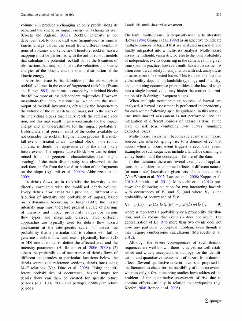
volume will produce a changing velocity profile along its

path, and the kinetic or impact energy will change as well

(Crosta and Agliardi 2003). Rockfall intensity is not

dependent solely on rockfall size (magnitude), as similar

kinetic energy values can result from different combina-

tions of volumes and velocities. Therefore, rockfall hazard

mapping must be performed with the aid of runout models

that calculate the potential rockfall paths, the locations of

obstructions that may stop blocks, the velocities and kinetic

energies of the blocks, and the spatial distribution of the

kinetic energy.

A critical issue is the definition of the characteristic

rockfall volume. In the case of fragmented rockfalls (Evans

and Hungr 1993), the hazard is caused by individual blocks

that follow more or less independent trajectories. However,

magnitude–frequency relationships, which are the usual

output of rockfall inventories, often link the frequency to

the volume of the initial detached mass, not to the sizes of

the individual blocks that finally reach the reference sec-

tion, and this may result in an overestimate for the impact

energy and an underestimate for the impact probability.

Unfortunately, at present, most of the codes available do

not consider the rockfall fragmentation process. If a rock-

fall event is treated as an individual block in the runout

analysis, it should be representative of the most likely

future events. The representative block size can be deter-

mined from the geometric characteristics (i.e. length,

spacing) of the main discontinuity sets observed on the

rock face, and/or from the size distribution of the fragments

on the slope (Agliardi et al. 2009b; Abbruzzese et al.

2009).

In debris flows, as in rockfalls, the intensity is not

directly correlated with the mobilised debris volume.

Every debris flow event will produce a different dis-

tribution of intensity and probability of impact, based

on its dynamics. According to Hungr (1997), the hazard

intensity map must therefore present a scale of pairings

of intensity and impact probability values for various

flow types and magnitude classes. Two different

approaches are typically used for debris flow hazard

assessment at the site-specific scale: (1) assess the

probability that a particular debris volume will fail to

generate a debris flow, and use a physically based (2D

or 3D) runout model to define the affected area and the

intensity parameters (Hurlimann et al. 2006, 2008); (2)

assess the probabilities of occurrence of debris flows of

different magnitudes at particular locations below the

debris source (i.e. reference sections, debris fans) using

M–F relations (Van Dine et al. 2005). Using the dif-

ferent probabilities of occurrence, hazard maps for

debris flows can then be created for specific return

periods (e.g. 100-, 500- and perhaps 2,500-year return

periods).

Landslide multi-hazard assessment

The term ‘‘multi-hazard’’ is frequently used in the literature

(Lewis 1984; Granger et al. 1999) as an adjective to indicate

multiple sources of hazard that are analysed in parallel and

finally integrated into a multi-risk analysis. Multi-hazard

assessment should, sensu stricto, refer to the joint probability

of independent events occurring in the same area in a given

time span. In practice, however, multi-hazard assessment is

often considered solely in conjunction with risk analysis, as

an assessment of expected losses. This is due to the fact that

vulnerability depends on landslide typology and intensity,

and combining occurrence probabilities at the hazard stage

into a single hazard value may hinder the correct determi-

nation of risk during subsequent stages.

When multiple noninteracting sources of hazard are

analysed, a hazard assessment is performed independently

for each source following specific guidance. In this sense, a

true multi-hazard assessment is not performed, and the

integration of different sources of hazard is done at the

level of risk (e.g. combining F–N curves, summing

expected losses).

Multi-hazard assessment becomes relevant when hazard

sources can interact, giving rise to a domino effect that

occurs when a hazard event triggers a secondary event.

Examples of such sequences include a landslide damming a

valley bottom and the consequent failure of the dam.

In the literature, there are several examples of applica-

tions that consider the combined effects of different natural

(or man-made) hazards on given sets of elements at risk

(Van Westen et al. 2002; Lacasse et al. 2008; Kappes et al.

2010; Schmidt et al. 2011). Marzocchi et al. (2012) pro-

poses the following equation for two interacting hazards

with occurrences of E1 and E2 (and where H1 is the

probability of occurrence of E1):

H1 ¼ p E1ð Þ ¼ p E1jE2ð Þp E2ð Þ þ p E1j �E2ð Þp �E2ð Þð Þ; ð9Þ

where p represents a probability or a probability distribu-

tion, and E2 means that event E2 does not occur. The

generalisation of Eq. 9 to more than two events does not

pose any particular conceptual problem, even though it

may require cumbersome calculations (Marzocchi et al.

2012).

Although the severe consequences of such domino

sequences are well known, there is, as yet, no well-estab-

lished and widely accepted methodology for the identifi-

cation and quantitative assessment of hazard from domino

effects. Several qualitative criteria have been proposed in

the literature to check for the possibility of domino events,

whereas only a few pioneering studies have addressed the

problem of the quantitative assessment of risk due to

domino effects—usually in relation to earthquakes (e.g.

Keefer 1984; Romeo et al. 2006).


123

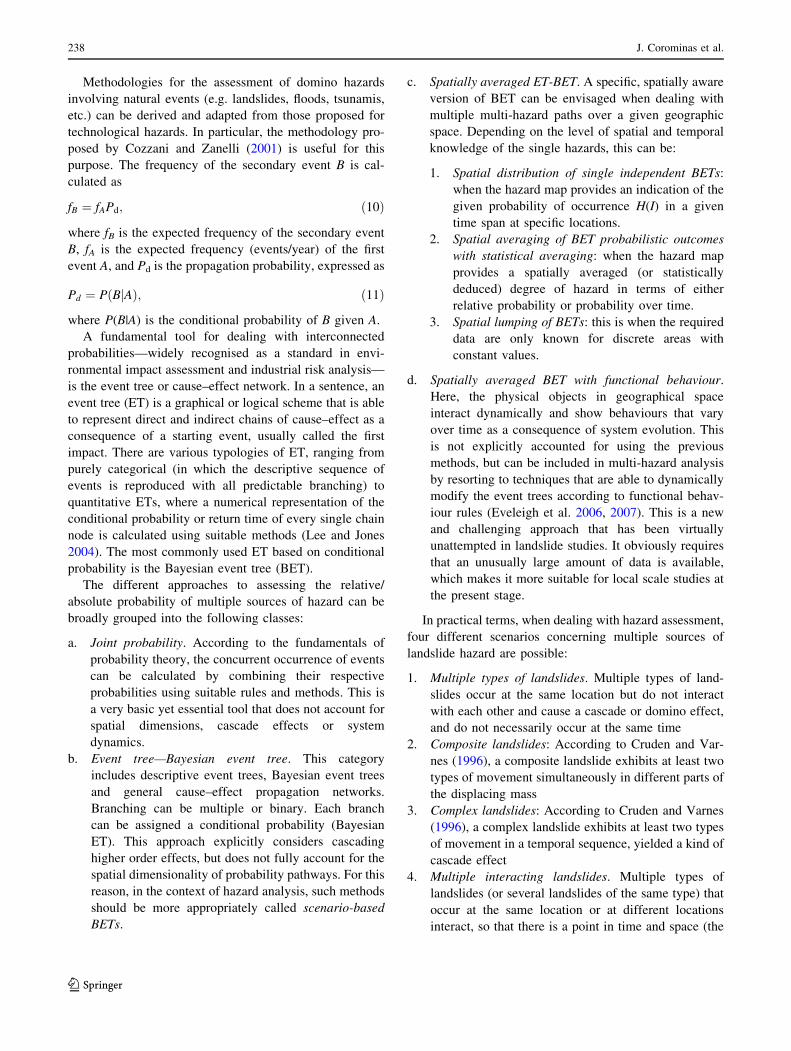
Methodologies for the assessment of domino hazards

involving natural events (e.g. landslides, floods, tsunamis,

etc.) can be derived and adapted from those proposed for

technological hazards. In particular, the methodology pro-

posed by Cozzani and Zanelli (2001) is useful for this

purpose. The frequency of the secondary event B is cal-

culated as

fB ¼ fAPd; ð10Þ

where fB is the expected frequency of the secondary event

B, fA is the expected frequency (events/year) of the first

event A, and Pd is the propagation probability, expressed as

Pd ¼ P BjAð Þ; ð11Þ

where P(B|A) is the conditional probability of B given A.

A fundamental tool for dealing with interconnected

probabilities—widely recognised as a standard in envi-

ronmental impact assessment and industrial risk analysis—

is the event tree or cause–effect network. In a sentence, an

event tree (ET) is a graphical or logical scheme that is able

to represent direct and indirect chains of cause–effect as a

consequence of a starting event, usually called the first

impact. There are various typologies of ET, ranging from

purely categorical (in which the descriptive sequence of

events is reproduced with all predictable branching) to

quantitative ETs, where a numerical representation of the

conditional probability or return time of every single chain

node is calculated using suitable methods (Lee and Jones

2004). The most commonly used ET based on conditional

probability is the Bayesian event tree (BET).

The different approaches to assessing the relative/

absolute probability of multiple sources of hazard can be

broadly grouped into the following classes:

a. Joint probability. According to the fundamentals of

probability theory, the concurrent occurrence of events

can be calculated by combining their respective

probabilities using suitable rules and methods. This is

a very basic yet essential tool that does not account for

spatial dimensions, cascade effects or system

dynamics.

b. Event tree—Bayesian event tree. This category

includes descriptive event trees, Bayesian event trees

and general cause–effect propagation networks.

Branching can be multiple or binary. Each branch

can be assigned a conditional probability (Bayesian

ET). This approach explicitly considers cascading

higher order effects, but does not fully account for the

spatial dimensionality of probability pathways. For this

reason, in the context of hazard analysis, such methods

should be more appropriately called scenario-based

BETs.

c. Spatially averaged ET-BET. A specific, spatially aware

version of BET can be envisaged when dealing with

multiple multi-hazard paths over a given geographic

space. Depending on the level of spatial and temporal

knowledge of the single hazards, this can be:

1. Spatial distribution of single independent BETs:

when the hazard map provides an indication of the

given probability of occurrence H(I) in a given

time span at specific locations.

2. Spatial averaging of BET probabilistic outcomes

with statistical averaging: when the hazard map

provides a spatially averaged (or statistically

deduced) degree of hazard in terms of either

relative probability or probability over time.

3. Spatial lumping of BETs: this is when the required

data are only known for discrete areas with

constant values.

d. Spatially averaged BET with functional behaviour.

Here, the physical objects in geographical space

interact dynamically and show behaviours that vary

over time as a consequence of system evolution. This

is not explicitly accounted for using the previous

methods, but can be included in multi-hazard analysis

by resorting to techniques that are able to dynamically

modify the event trees according to functional behav-

iour rules (Eveleigh et al. 2006, 2007). This is a new

and challenging approach that has been virtually

unattempted in landslide studies. It obviously requires

that an unusually large amount of data is available,

which makes it more suitable for local scale studies at

the present stage.

In practical terms, when dealing with hazard assessment,

four different scenarios concerning multiple sources of

landslide hazard are possible:

1. Multiple types of landslides. Multiple types of land-

slides occur at the same location but do not interact

with each other and cause a cascade or domino effect,

and do not necessarily occur at the same time

2. Composite landslides: According to Cruden and Var-

nes (1996), a composite landslide exhibits at least two

types of movement simultaneously in different parts of

the displacing mass

3. Complex landslides: According to Cruden and Varnes

(1996), a complex landslide exhibits at least two types

of movement in a temporal sequence, yielded a kind of

cascade effect

4. Multiple interacting landslides. Multiple types of

landslides (or several landslides of the same type) that

occur at the same location or at different locations

interact, so that there is a point in time and space (the


123

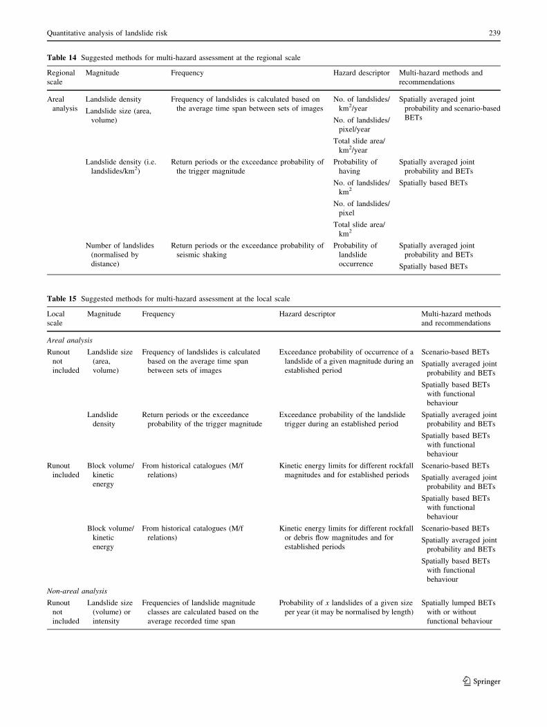
Table 14 Suggested methods for multi-hazard assessment at the regional scale

Regional

scale

Magnitude Frequency Hazard descriptor Multi-hazard methods and

recommendations

Areal

analysis

Landslide density

Landslide size (area,

volume)

Frequency of landslides is calculated based on

the average time span between sets of images

No. of landslides/

km2/year

No. of landslides/

pixel/year

Total slide area/

km2/year

Spatially averaged joint

probability and scenario-based

BETs

Landslide density (i.e.

landslides/km2)

Return periods or the exceedance probability of

the trigger magnitude

Probability of

having

No. of landslides/

km2

No. of landslides/

pixel

Total slide area/

km2


probability and BETs

Spatially based BETs

Number of landslides

(normalised by

distance)

Return periods or the exceedance probability of

seismic shaking

Probability of

landslide

occurrence




Table 15 Suggested methods for multi-hazard assessment at the local scale

Local

scale

Magnitude Frequency Hazard descriptor Multi-hazard methods

and recommendations

Areal analysis

Runout

not

included

Landslide size

(area,

volume)

Frequency of landslides is calculated

based on the average time span

between sets of images

Exceedance probability of occurrence of a

landslide of a given magnitude during an

established period

Scenario-based BETs




with functional

behaviour

Landslide

density

Return periods or the exceedance

probability of the trigger magnitude

Exceedance probability of the landslide

trigger during an established period




with functional

behaviour

Runout

included

Block volume/

kinetic

energy

From historical catalogues (M/f

relations)

Kinetic energy limits for different rockfall

magnitudes and for established periods

Scenario-based BETs




with functional

behaviour

Block volume/

kinetic

energy

From historical catalogues (M/f

relations)

Kinetic energy limits for different rockfall

or debris flow magnitudes and for

established periods

Scenario-based BETs




with functional

behaviour

Non-areal analysis

Runout

not

included

Landslide size

(volume) or

intensity

Frequencies of landslide magnitude

classes are calculated based on the

average recorded time span

Probability of x landslides of a given size

per year (it may be normalised by length)

Spatially lumped BETs

with or without

functional behaviour


123

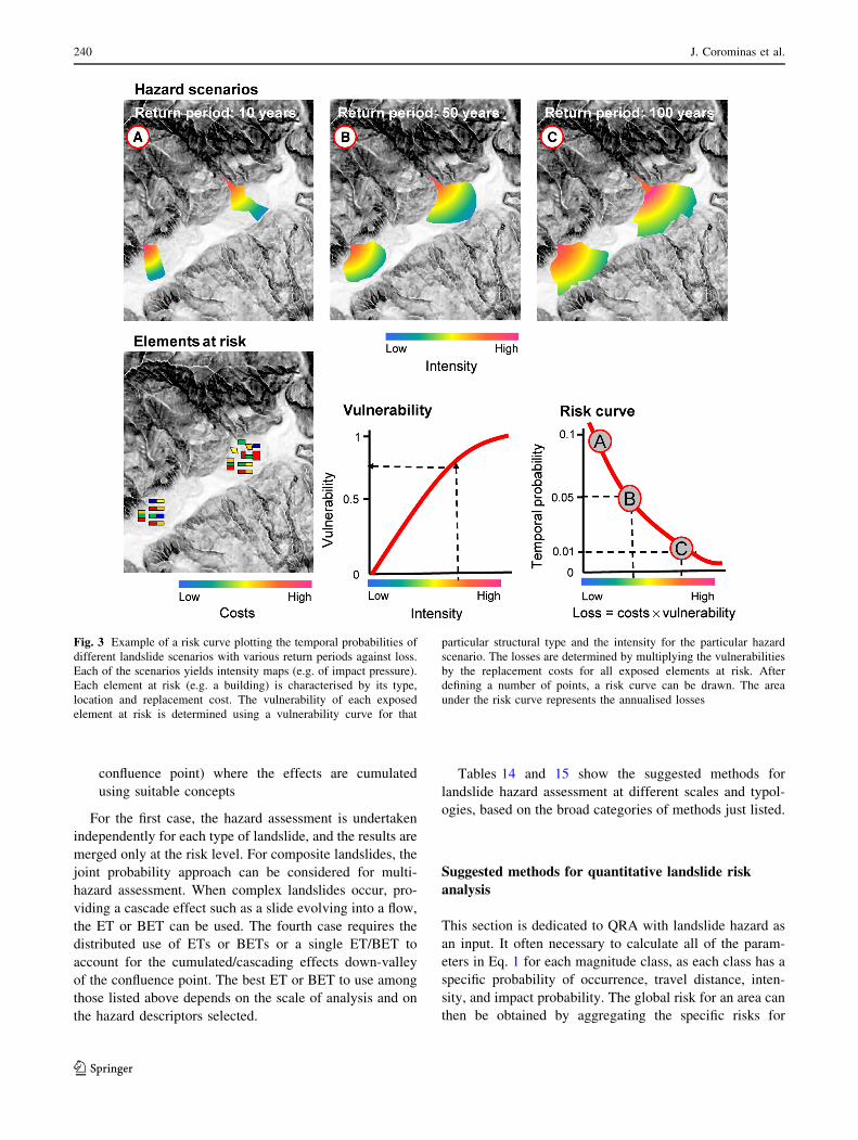
confluence point) where the effects are cumulated

using suitable concepts

For the first case, the hazard assessment is undertaken

independently for each type of landslide, and the results are

merged only at the risk level. For composite landslides, the

joint probability approach can be considered for multi-

hazard assessment. When complex landslides occur, pro-

viding a cascade effect such as a slide evolving into a flow,

the ET or BET can be used. The fourth case requires the

distributed use of ETs or BETs or a single ET/BET to

account for the cumulated/cascading effects down-valley

of the confluence point. The best ET or BET to use among

those listed above depends on the scale of analysis and on

the hazard descriptors selected.

Tables 14 and 15 show the suggested methods for

landslide hazard assessment at different scales and typol-

ogies, based on the broad categories of methods just listed.

Suggested methods for quantitative landslide risk

analysis

This section is dedicated to QRA with landslide hazard as

an input. It often necessary to calculate all of the param-

eters in Eq. 1 for each magnitude class, as each class has a

specific probability of occurrence, travel distance, inten-

sity, and impact probability. The global risk for an area can

then be obtained by aggregating the specific risks for

Fig. 3 Example of a risk curve plotting the temporal probabilities of

different landslide scenarios with various return periods against loss.

Each of the scenarios yields intensity maps (e.g. of impact pressure).

Each element at risk (e.g. a building) is characterised by its type,

location and replacement cost. The vulnerability of each exposed

element at risk is determined using a vulnerability curve for that

particular structural type and the intensity for the particular hazard

scenario. The losses are determined by multiplying the vulnerabilities

by the replacement costs for all exposed elements at risk. After

defining a number of points, a risk curve can be drawn. The area

under the risk curve represents the annualised losses


123

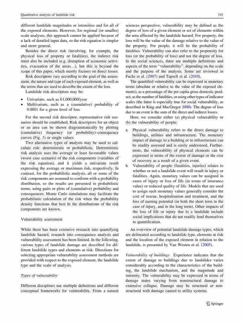
different landslide magnitudes or intensities and for all of

the exposed elements. However, for regional (or smaller)

scale analyses, this approach cannot be applied because of

a lack of detailed input data, so the risk equation is simpler

and more general.

Besides the direct risk (involving, for example, the

physical loss of property or fatalities), the indirect risk

must also be included (e.g. disruption of economic activi-

ties, evacuation of the areas…), but this is beyond the

scope of this paper, which mostly focuses on direct losses.

Risk descriptors vary according to the goal of the assess-

ment, the nature and type of each exposed element, as well as

the terms that are used to describe the extent of the loss.

Landslide risk descriptors may be:

• Univariate, such as €1,000,000/year

• Multivariate, such as a (cumulative) probability of

0.0001 for a given level of loss

For the second risk descriptor, representative risk sce-

narios should be established. Risk descriptors for an object

or an area can be shown diagrammatically by plotting

(cumulative) frequency (or probability)–consequence

curves (Fig. 3) or single values.

Two alternative types of analysis may be used to cal-

culate risk: deterministic or probabilistic. Deterministic

risk analysis uses the average or least favourable values

(worst case scenario) of the risk components (variables of

the risk equation), and it yields a univariate result

expressing the average or maximum risk, respectively. In

contrast, for the probabilistic analysis, all or some of the

risk components are assumed to conform with a probability

distribution, so the results are presented in probabilistic

terms, using pairs or plots of (cumulative) probability and

consequences. Monte Carlo simulations may facilitate the

probabilistic calculation of the risk when the probability

density functions that best fit the distributions of the risk

components are known.

Vulnerability assessment

While there has been extensive research into quantifying

landslide hazard, research into consequence analysis and

vulnerability assessment has been limited. In the following,

various types of landslide damage are described for dif-

ferent landslide types and elements at risk. Directions for

selecting appropriate vulnerability assessment methods are

provided with respect to the exposed element, the landslide

type and the scale of analysis.

Types of vulnerability

Different disciplines use multiple definitions and different

conceptual frameworks for vulnerability. From a natural

sciences perspective, vulnerability may be defined as the

degree of loss of a given element or set of elements within

the area affected by the landslide hazard. For property, the

loss will be the value of the damage relative to the value of

the property. For people, it will be the probability of

fatalities. Vulnerability can also refer to the propensity for

loss (or the probability of loss) and not the degree of loss.

In the social sciences, there are multiple definitions and

aspects of the term ‘‘vulnerability’’, depending on the scale

and the purpose of the analysis. Some are reviewed in

Fuchs et al. (2007) and Tapsell et al. (2010).

The quantified vulnerability can be expressed in monetary

terms (absolute or relative to the value of the exposed ele-

ments), as a percentage of the per capita gross domestic prod-

uct, as the number of fatalities, or using other types of indicator

scales (the latter is especially true for social vulnerability, as

described in King and MacGregor 2000). The degree of loss

due to an event is the sum of the direct and indirect losses.

Here, we consider either (a) physical vulnerability or

(b) the vulnerability of people:

a. Physical vulnerability refers to the direct damage to

buildings, utilities and infrastructure. The monetary

impact of damage to a building or to infrastructure can

be readily assessed and is easily understood. Further-

more, the vulnerability of physical elements can be

expressed in terms of the extent of damage or the cost

of recovery as a result of a given event.

b. Vulnerability of people (fatalities, injuries) relates to

whether or not a landslide event will result in injury or

fatalities. Again, monetary values can be assigned in

cases of injury or loss of life (in terms of insurance

value) or reduced quality of life. Models that are used

to assign such monetary values generally consider the

cost of rescue, hospitalisation and treatment, and the

loss of earning potential (in both the short term in the

case of injury, and in the long term). Other impacts of

the loss of life or injury due to a landslide include

social implications that do not readily lend themselves

to quantification.

An overview of potential landslide damage types, which

are delineated according to landslide type, elements at risk

and the location of the exposed element in relation to the

landslide, is presented by Van Westen et al. (2005).

Vulnerability of buildings Experience indicates that the

extent of damage to buildings due to landslides varies

considerably according to the characteristics of the build-

ing, the landslide mechanism, and the magnitude and

intensity. The vulnerability may be expressed in terms of

damage states varying from nonstructural damage to

extensive collapse. Damage may be structural or non-

structural with damage caused to utility systems.


123

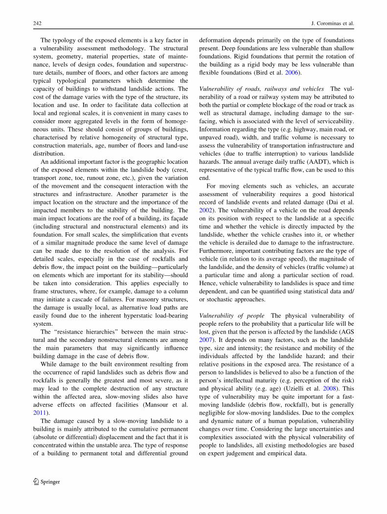
The typology of the exposed elements is a key factor in

a vulnerability assessment methodology. The structural

system, geometry, material properties, state of mainte-

nance, levels of design codes, foundation and superstruc-

ture details, number of floors, and other factors are among

typical typological parameters which determine the

capacity of buildings to withstand landslide actions. The

cost of the damage varies with the type of the structure, its

location and use. In order to facilitate data collection at

local and regional scales, it is convenient in many cases to

consider more aggregated levels in the form of homoge-

neous units. These should consist of groups of buildings,

characterised by relative homogeneity of structural type,

construction materials, age, number of floors and land-use

distribution.

An additional important factor is the geographic location

of the exposed elements within the landslide body (crest,

transport zone, toe, runout zone, etc.), given the variation

of the movement and the consequent interaction with the

structures and infrastructure. Another parameter is the

impact location on the structure and the importance of the

impacted members to the stability of the building. The

main impact locations are the roof of a building, its facade

(including structural and nonstructural elements) and its

foundation. For small scales, the simplification that events

of a similar magnitude produce the same level of damage

can be made due to the resolution of the analysis. For

detailed scales, especially in the case of rockfalls and

debris flow, the impact point on the building—particularly

on elements which are important for its stability—should

be taken into consideration. This applies especially to

frame structures, where, for example, damage to a column

may initiate a cascade of failures. For masonry structures,

the damage is usually local, as alternative load paths are

easily found due to the inherent hyperstatic load-bearing

system.

The ‘‘resistance hierarchies’’ between the main struc-

tural and the secondary nonstructural elements are among

the main parameters that may significantly influence

building damage in the case of debris flow.

While damage to the built environment resulting from

the occurrence of rapid landslides such as debris flow and

rockfalls is generally the greatest and most severe, as it

may lead to the complete destruction of any structure

within the affected area, slow-moving slides also have

adverse effects on affected facilities (Mansour et al.

2011).

The damage caused by a slow-moving landslide to a

building is mainly attributed to the cumulative permanent

(absolute or differential) displacement and the fact that it is

concentrated within the unstable area. The type of response

of a building to permanent total and differential ground

deformation depends primarily on the type of foundations

present. Deep foundations are less vulnerable than shallow

foundations. Rigid foundations that permit the rotation of

the building as a rigid body may be less vulnerable than

flexible foundations (Bird et al. 2006).

Vulnerability of roads, railways and vehicles The vul-

nerability of a road or railway system may be attributed to

both the partial or complete blockage of the road or track as

well as structural damage, including damage to the sur-

facing, which is associated with the level of serviceability.

Information regarding the type (e.g. highway, main road, or

unpaved road), width, and traffic volume is necessary to

assess the vulnerability of transportation infrastructure and

vehicles (due to traffic interruption) to various landslide

hazards. The annual average daily traffic (AADT), which is

representative of the typical traffic flow, can be used to this

end.

For moving elements such as vehicles, an accurate

assessment of vulnerability requires a good historical

record of landslide events and related damage (Dai et al.

2002). The vulnerability of a vehicle on the road depends

on its position with respect to the landslide at a specific

time and whether the vehicle is directly impacted by the

landslide, whether the vehicle crashes into it, or whether

the vehicle is derailed due to damage to the infrastructure.

Furthermore, important contributing factors are the type of

vehicle (in relation to its average speed), the magnitude of

the landslide, and the density of vehicles (traffic volume) at

a particular time and along a particular section of road.

Hence, vehicle vulnerability to landslides is space and time

dependent, and can be quantified using statistical data and/

or stochastic approaches.

Vulnerability of people The physical vulnerability of

people refers to the probability that a particular life will be

lost, given that the person is affected by the landslide (AGS

2007). It depends on many factors, such as the landslide

type, size and intensity; the resistance and mobility of the

individuals affected by the landslide hazard; and their

relative positions in the exposed area. The resistance of a

person to landslides is believed to also be a function of the

person’s intellectual maturity (e.g. perception of the risk)

and physical ability (e.g. age) (Uzielli et al. 2008). This

type of vulnerability may be quite important for a fast-

moving landslide (debris flow, rockfall), but is generally

negligible for slow-moving landslides. Due to the complex

and dynamic nature of a human population, vulnerability

changes over time. Considering the large uncertainties and

complexities associated with the physical vulnerability of

people to landslides, all existing methodologies are based

on expert judgement and empirical data.


123

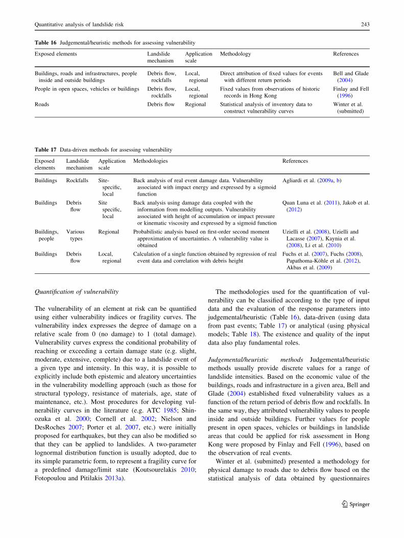
Quantification of vulnerability

The vulnerability of an element at risk can be quantified

using either vulnerability indices or fragility curves. The

vulnerability index expresses the degree of damage on a

relative scale from 0 (no damage) to 1 (total damage).

Vulnerability curves express the conditional probability of

reaching or exceeding a certain damage state (e.g. slight,

moderate, extensive, complete) due to a landslide event of

a given type and intensity. In this way, it is possible to

explicitly include both epistemic and aleatory uncertainties

in the vulnerability modelling approach (such as those for

structural typology, resistance of materials, age, state of

maintenance, etc.). Most procedures for developing vul-

nerability curves in the literature (e.g. ATC 1985; Shin-

ozuka et al. 2000; Cornell et al. 2002; Nielson and

DesRoches 2007; Porter et al. 2007, etc.) were initially

proposed for earthquakes, but they can also be modified so

that they can be applied to landslides. A two-parameter

lognormal distribution function is usually adopted, due to

its simple parametric form, to represent a fragility curve for

a predefined damage/limit state (Koutsourelakis 2010;

Fotopoulou and Pitilakis 2013a).

The methodologies used for the quantification of vul-

nerability can be classified according to the type of input

data and the evaluation of the response parameters into

judgemental/heuristic (Table 16), data-driven (using data

from past events; Table 17) or analytical (using physical

models; Table 18). The existence and quality of the input

data also play fundamental roles.

Judgemental/heuristic methods Judgemental/heuristic

methods usually provide discrete values for a range of

landslide intensities. Based on the economic value of the

buildings, roads and infrastructure in a given area, Bell and

Glade (2004) established fixed vulnerability values as a

function of the return period of debris flow and rockfalls. In

the same way, they attributed vulnerability values to people

inside and outside buildings. Further values for people

present in open spaces, vehicles or buildings in landslide

areas that could be applied for risk assessment in Hong

Kong were proposed by Finlay and Fell (1996), based on

the observation of real events.

Winter et al. (submitted) presented a methodology for

physical damage to roads due to debris flow based on the

statistical analysis of data obtained by questionnaires

Table 16 Judgemental/heuristic methods for assessing vulnerability

Exposed elements Landslide

mechanism

Application

scale

Methodology References

Buildings, roads and infrastructures, people

inside and outside buildings

Debris flow,

rockfalls

Local,

regional

Direct attribution of fixed values for events

with different return periods

Bell and Glade

(2004)

People in open spaces, vehicles or buildings Debris flow,

rockfalls

Local,

regional

Fixed values from observations of historic

records in Hong Kong

Finlay and Fell

(1996)

Roads Debris flow Regional Statistical analysis of inventory data to

construct vulnerability curves

Winter et al.

(submitted)

Table 17 Data-driven methods for assessing vulnerability

Exposed

elements

Landslide

mechanism

Application

scale

Methodologies References

Buildings Rockfalls Site-

specific,

local

Back analysis of real event damage data. Vulnerability

associated with impact energy and expressed by a sigmoid

function

Agliardi et al. (2009a, b)

Buildings Debris

flow

Site

specific,

local

Back analysis using damage data coupled with the

information from modelling outputs. Vulnerability

associated with height of accumulation or impact pressure

or kinematic viscosity and expressed by a sigmoid function

Quan Luna et al. (2011), Jakob et al.

(2012)

Buildings,

people

Various

types

Regional Probabilistic analysis based on first-order second moment

approximation of uncertainties. A vulnerability value is

obtained

Uzielli et al. (2008), Uzielli and

Lacasse (2007), Kaynia et al.

(2008), Li et al. (2010)

Buildings Debris

flow

Local,

regional

Calculation of a single function obtained by regression of real

event data and correlation with debris height

Fuchs et al. (2007), Fuchs (2008),

Papathoma-Kohle et al. (2012),

Akbas et al. (2009)


123

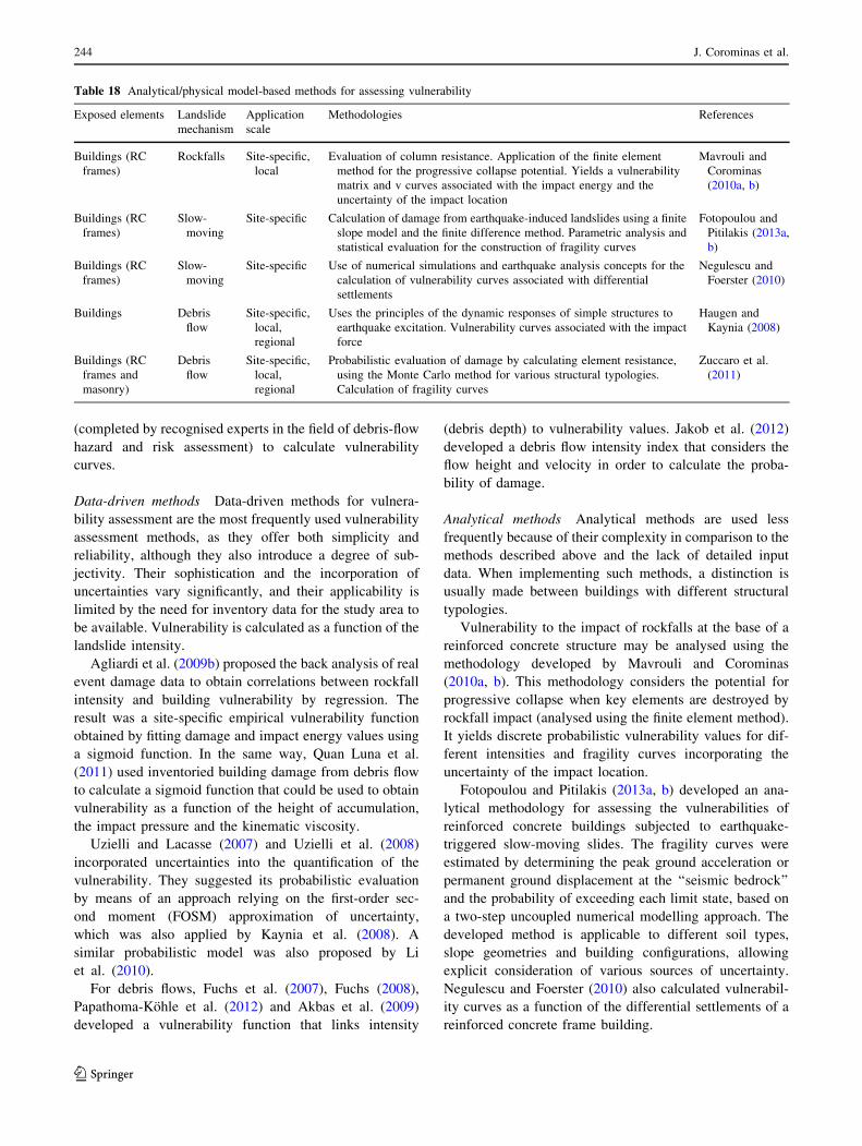
(completed by recognised experts in the field of debris-flow

hazard and risk assessment) to calculate vulnerability

curves.

Data-driven methods Data-driven methods for vulnera-

bility assessment are the most frequently used vulnerability

assessment methods, as they offer both simplicity and

reliability, although they also introduce a degree of sub-

jectivity. Their sophistication and the incorporation of

uncertainties vary significantly, and their applicability is

limited by the need for inventory data for the study area to

be available. Vulnerability is calculated as a function of the

landslide intensity.

Agliardi et al. (2009b) proposed the back analysis of real

event damage data to obtain correlations between rockfall

intensity and building vulnerability by regression. The

result was a site-specific empirical vulnerability function

obtained by fitting damage and impact energy values using

a sigmoid function. In the same way, Quan Luna et al.

(2011) used inventoried building damage from debris flow

to calculate a sigmoid function that could be used to obtain

vulnerability as a function of the height of accumulation,

the impact pressure and the kinematic viscosity.

Uzielli and Lacasse (2007) and Uzielli et al. (2008)

incorporated uncertainties into the quantification of the

vulnerability. They suggested its probabilistic evaluation

by means of an approach relying on the first-order sec-

ond moment (FOSM) approximation of uncertainty,

which was also applied by Kaynia et al. (2008). A

similar probabilistic model was also proposed by Li

et al. (2010).

For debris flows, Fuchs et al. (2007), Fuchs (2008),

Papathoma-Kohle et al. (2012) and Akbas et al. (2009)

developed a vulnerability function that links intensity

(debris depth) to vulnerability values. Jakob et al. (2012)

developed a debris flow intensity index that considers the

flow height and velocity in order to calculate the proba-

bility of damage.

Analytical methods Analytical methods are used less

frequently because of their complexity in comparison to the

methods described above and the lack of detailed input

data. When implementing such methods, a distinction is

usually made between buildings with different structural

typologies.

Vulnerability to the impact of rockfalls at the base of a

reinforced concrete structure may be analysed using the

methodology developed by Mavrouli and Corominas

(2010a, b). This methodology considers the potential for

progressive collapse when key elements are destroyed by

rockfall impact (analysed using the finite element method).

It yields discrete probabilistic vulnerability values for dif-

ferent intensities and fragility curves incorporating the

uncertainty of the impact location.

Fotopoulou and Pitilakis (2013a, b) developed an ana-

lytical methodology for assessing the vulnerabilities of

reinforced concrete buildings subjected to earthquake-

triggered slow-moving slides. The fragility curves were

estimated by determining the peak ground acceleration or

permanent ground displacement at the ‘‘seismic bedrock’’

and the probability of exceeding each limit state, based on

a two-step uncoupled numerical modelling approach. The

developed method is applicable to different soil types,

slope geometries and building configurations, allowing

explicit consideration of various sources of uncertainty.

Negulescu and Foerster (2010) also calculated vulnerabil-

ity curves as a function of the differential settlements of a

reinforced concrete frame building.

Table 18 Analytical/physical model-based methods for assessing vulnerability

Exposed elements Landslide

mechanism

Application

scale

Methodologies References

Buildings (RC

frames)

Rockfalls Site-specific,

local

Evaluation of column resistance. Application of the finite element

method for the progressive collapse potential. Yields a vulnerability

matrix and v curves associated with the impact energy and the

uncertainty of the impact location

Mavrouli and

Corominas

(2010a, b)

Buildings (RC

frames)

Slow-

moving

Site-specific Calculation of damage from earthquake-induced landslides using a finite

slope model and the finite difference method. Parametric analysis and

statistical evaluation for the construction of fragility curves

Fotopoulou and

Pitilakis (2013a,

b)

Buildings (RC

frames)

Slow-

moving

Site-specific Use of numerical simulations and earthquake analysis concepts for the

calculation of vulnerability curves associated with differential

settlements

Negulescu and

Foerster (2010)

Buildings Debris

flow

Site-specific,

local,

regional

Uses the principles of the dynamic responses of simple structures to

earthquake excitation. Vulnerability curves associated with the impact

force

Haugen and

Kaynia (2008)

Buildings (RC

frames and

masonry)

Debris

flow

Site-specific,

local,

regional

Probabilistic evaluation of damage by calculating element resistance,

using the Monte Carlo method for various structural typologies.

Calculation of fragility curves

Zuccaro et al.

(2011)


123

Vulnerability curves may be produced for unreinforced

masonry structures and reinforced masonry structures that

are subjected to debris flows using the method proposed by

Haugen and Kaynia (2008), which implements the HAZUS

software package (NIBS 2004). This method uses the

principles of the dynamic response of a simple structure to

earthquake excitation. Additionally, Zuccaro et al. (2011)

presented another analytical method for calculating vul-

nerability curves that is based on the resistances of a

reinforced concrete RC frame and the infill wall, in prob-

abilistic terms, and uses Monte Carlo simulation. The

resistance hierarchy among the distinct elements is taken

into consideration.

Risk analysis

The risk—in a similar manner to the hazard—may refer to

a single object, a linear feature or an area. Areal analysis is

usually required by local and regional governments for the

purposes of land planning or the design of protection

measures. It is very demanding in terms of the data

required to calculate the hazard and the vulnerability

parameters, and it imposes many restrictions on the

detailed runout analysis that can be performed as well as

the incorporation of landslide kinematics. The areal ana-

lysis is typically performed at a regional scale and imple-

mented in GIS platforms, with maps being used to illustrate

the risk (Agliardi et al. 2009b). The latter may be expressed

as the annual monetary loss per pixel or area unit, or as the

probability of a given risk scenario (Remondo et al. 2005).

Risk analysis for linear features, for example roads or

railways, is a very common procedure. The risk may be

calculated either for the entire line or some selected parts,

specifically those that are most at risk. This analysis does

not necessarily require an assessment of the frequency at

the source area, but the inventory of the events that reach

the infrastructure should be as complete as possible. On the

other hand, if the landslide occurrence is evaluated at the

source, propagation analysis is needed (Roberds 2005).

Even though the landslide intensity best expresses the

damage potential of the landslide, it is rarely considered in

this type of analysis (Bunce et al. 1997; Hungr et al. 1999).

Object-orientated analysis is performed for buildings,

road cuts or specific facilities. Landslide analysis is usually

undertaken using analytical and/or numerical models, and

includes the calculation of the spatial parameters that

influence the probability of a landslide of a given magni-

tude or velocity reaching the exposed element(s). Restric-

tions in this case may stem from the scarcity of the data

needed to properly assess the probability or frequency of

occurrence. Risk may be expressed as the annual monetary

loss per object or the annual probability of property dam-

age or loss of life for different risk scenarios.

Exposure

Exposure is an attribute of people, property, systems or

other elements present in areas that are potentially affected

by landslides. It is calculated as the temporal and spatial

probability that an element at risk is within the landslide

path, and it also needs to be incorporated into the risk

equation. The calculation of the exposure depends mainly

on the scale of the analysis and the type of element

potentially exposed. Whether an element is exposed or not

is determined by its location with respect to the landslide

path, which varies according to the landslide mechanism.

For exposure, there is an important distinction between

static elements (buildings, roads, other infrastructure, etc.)

and moving elements (vehicles, persons, etc.).

Static elements In the case of rockfalls, the affected ele-

ments are located within the rockfall path. Exposed ele-

ments for fragmented rockfalls have limited spatial

intersections, while the intersections are larger for rock

avalanches and rockslides. For fragmented rockfalls, and at

small scales with low resolution, all of the elements next to

rockfall-prone cliffs are assumed to be exposed. At site-

specific and local scales, and when the trajectory is inclu-

ded in the analysis, this is limited to only the elements that

are situated within the potential rockfall path. In the latter

case, the exposure component varies as a function of the

block size.

The impact probability may be obtained by considering

the percentage of the area that contains structures in one or

more reference sections reached by the rockfall path

(Corominas et al. 2005; Corominas and Mavrouli 2011b).

For large-scale analyses, where detailed information on the

spatial probability of a block reaching a building is

required, the probabilities of individual block trajectories

may be computed. Some rockfall sources produce paths

that have a higher probability of affecting some buildings

than others do, and this has to be taken into account.

Debris flows can affect larger areas than rockfalls, due

to their increased mobility and possibility of inundation. In

some cases, deposition affects an entire urban area. The

spatial exposure of an area can be calculated as the ratio of

the affected area to the total area. Whether the latter is

calculated as a function of the flow kinematics (e.g. dis-

charge rate) or not depends on the availability of propa-

gation information at the scale of analysis considered, as

previously mentioned.

For slow-moving landslides, the exposed elements may

be located on it, next to the landslide scarp or in the

landslide runout zone. Because of this, the actions applied

and the damage caused may vary. Again, the exposure of

each element may be calculated as a function of the


123

landslide kinematics if the scale and the resolution of the

analysis permit this.

Kinematic analysis is required to calculate the exposures

of linear elements such as roads and railways when the

frequency or probability of landslide occurrence is calcu-

lated at the source. If it is calculated to intersect directly

with the infrastructure, the exposure is equal to 1.

Moving elements Quantification of the temporal and

spatial probabilities of moving elements must take into

account the characteristics of their movement. Vehicles

may be exposed to landslides in different ways. They may

be affected while stationary or moving. They may be hit by

a rock or soil mass, or they may crash into a rock or soil

mass that is obstructing or blocking the road. Vehicles that

are buried or become entrained in the debris flow or

landslide, and thus become part of the moving mass, should

also be considered.

The impact probability can be calculated for the direct

impact of rocks or soil on vehicles. This depends, amongst

other factors, upon the frequency of the vehicles, the size of

the fragmented rock or the geometrical characteristics of

the debris flow or landslide, and the lengths of the vehicles.

Basic simplifying assumptions that are usually made for

the exposure of vehicles are that they are uniformly dis-

tributed temporally and spatially, and that all vehicles have

the same length (Bunce et al. 1997).

The temporal and spatial probability that a moving rock

or soil mass will intersect with a particular stationary

vehicle is proportional to the length of the infrastructure

occupied by the vehicle. For multiple events, the proba-

bility that no vehicle is hit is equal to

PðSÞ ¼ 1� 1� P S : Hð Þð ÞNr ; ð12Þ

where P(S:H) is the probability that a vehicle occupies the

portion of the road affected by a landslide, and Nr is the

number of events.

For a particular moving vehicle, the temporal probabil-

ity of intersection is also calculated as a function of the

occupying time, which depends on the frequency of the

moving vehicle as well as its average length and speed. The

width of the rock or the soil mass is usually neglected.

People are also affected by landslides in open spaces and

while occupying buildings and vehicles. In this context, the

temporal and spatial probability of intersection of a person

is calculated as a function of the exposure of the building or

vehicle the person is occupying and the percentage of time

and/or space that they spend in it (Fell et al. 2005). Thus,

for people inside buildings, the probability of intersection

depends on their usage of the building and their occupancy

of it during specific time spans. In some cases (ski resorts

for example) where the population varies between seasons,

the seasonal exposure should also be taken into account.

Risk analysis can be performed for either the most exposed

people or for those with the average exposure.

Risk calculation

Examples of the applications of QRA are summarised in

Table 19; although the risk components are not calculated

in a strictly quantitative manner in some of these applica-

tions, the proposed methodologies do yield quantitative

results.

Practical examples at site-specific and local scales are

provided in the literature for people inside vehicles during

rockfalls (Fell et al. 2005) and debris flows (Archetti and

Lamberti 2003; Budetta 2002). Wilson et al. (2005) con-

sider both the direct impact of debris on vehicles and the

risk of the vehicles running into the debris. The case study

of Jakob and Weatherly (2005) also describes the calcu-

lation of frequency–fatality curves for people; in that work,

vulnerability is calculated empirically from past data as a

function of the debris discharge rate. The procedure pre-

sented by Bell and Glade (2004) can be used at a regional

scale for risk analyses of buildings in relation to both debris

flows and rockfalls; this procedure is mainly based on

judgemental and empirical data.

If we consider more detailed scales, Agliardi et al.

(2009a, b) developed an analytical procedure for QRA

relating to rockfalls based on data from the back analysis of

a real rockfall event, which included data on the damage to

buildings. Corominas et al. (2005) showed an example of

the quantification of the risk of blocks hitting people inside

buildings. A methodology for the analysis of rockfall risk

for buildings for application at the site-specific scale was

proposed by Corominas and Mavrouli (2011a), which

included the analytical probabilistic vulnerability of

buildings as a function of the location of rock block impact.

Ferlisi et al. (2012) provided a methodology for calculating

the risk taken by people moving along a road while inside

vehicles.

For slow-moving landslides (amongst other types), Ca-

tani et al. (2005) proposed a methodology that yields

results in terms of the expected economic losses relating to

buildings, which used remote sensing techniques.

Finally, Ho et al. (2000) and Lee and Jones (2004)

presented practical cases of risk calculation for a range of

landslide types and exposed elements, with emphasis

placed on the calculation of F–N curves.

Risk scenarios

In a study area of a particular geo-environmental context,

the different stages of movement of existing or potential

landslide phenomena of a given type are controlled by

mechanisms that are often interrelated (Leroueil et al.


123

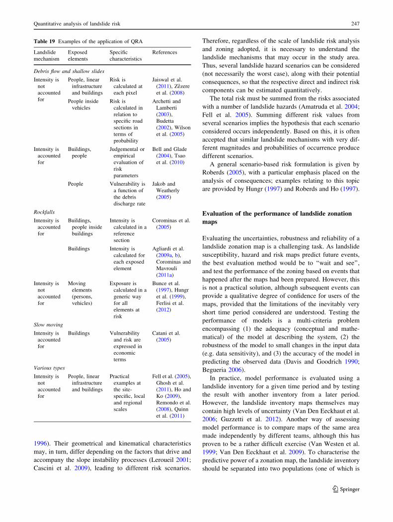
1996). Their geometrical and kinematical characteristics

may, in turn, differ depending on the factors that drive and

accompany the slope instability processes (Leroueil 2001;

Cascini et al. 2009), leading to different risk scenarios.

Therefore, regardless of the scale of landslide risk analysis

and zoning adopted, it is necessary to understand the

landslide mechanisms that may occur in the study area.

Thus, several landslide hazard scenarios can be considered

(not necessarily the worst case), along with their potential

consequences, so that the respective direct and indirect risk

components can be estimated quantitatively.

The total risk must be summed from the risks associated

with a number of landslide hazards (Amatruda et al. 2004;

Fell et al. 2005). Summing different risk values from

several scenarios implies the hypothesis that each scenario

considered occurs independently. Based on this, it is often

accepted that similar landslide mechanisms with very dif-

ferent magnitudes and probabilities of occurrence produce

different scenarios.

A general scenario-based risk formulation is given by

Roberds (2005), with a particular emphasis placed on the

analysis of consequences; examples relating to this topic

are provided by Hungr (1997) and Roberds and Ho (1997).

Evaluation of the performance of landslide zonation

maps

Evaluating the uncertainties, robustness and reliability of a

landslide zonation map is a challenging task. As landslide

susceptibility, hazard and risk maps predict future events,

the best evaluation method would be to ‘‘wait and see’’,

and test the performance of the zoning based on events that

happened after the maps had been prepared. However, this

is not a practical solution, although subsequent events can

provide a qualitative degree of confidence for users of the

maps, provided that the limitations of the inevitably very

short time period considered are understood. Testing the

performance of models is a multi-criteria problem

encompassing (1) the adequacy (conceptual and mathe-

matical) of the model at describing the system, (2) the

robustness of the model to small changes in the input data

(e.g. data sensitivity), and (3) the accuracy of the model in

predicting the observed data (Davis and Goodrich 1990;

Begueria 2006).

In practice, model performance is evaluated using a

landslide inventory for a given time period and by testing

the result with another inventory from a later period.

However, the landslide inventory maps themselves may

contain high levels of uncertainty (Van Den Eeckhaut et al.

2006; Guzzetti et al. 2012). Another way of assessing

model performance is to compare maps of the same area

made independently by different teams, although this has

proven to be a rather difficult exercise (Van Westen et al.

1999; Van Den Eeckhaut et al. 2009). To characterise the

predictive power of a zonation map, the landslide inventory

should be separated into two populations (one of which is

Table 19 Examples of the application of QRA

Landslide

mechanism

Exposed

elements

Specific

characteristics

References

Debris flow and shallow slides

Intensity is

not

accounted

for

People, linear

infrastructure

and buildings

Risk is

calculated at

each pixel

Jaiswal et al.

(2011), Zezere

et al. (2008)

People inside

vehicles

Risk is

calculated in

relation to

specific road

sections in

terms of

probability

Archetti and

Lamberti

(2003),

Budetta

(2002), Wilson

et al. (2005)

Intensity is

accounted

for

Buildings,

people

Judgemental or

empirical

evaluation of

risk

parameters

Bell and Glade

(2004), Tsao

et al. (2010)

People Vulnerability is

a function of

the debris

discharge rate

Jakob and

Weatherly

(2005)

Rockfalls

Intensity is

accounted

for

Buildings,

people inside

buildings

Intensity is

calculated in a

reference

section

Corominas et al.

(2005)

Buildings Intensity is

calculated for

each exposed

element

Agliardi et al.

(2009a, b),

Corominas and

Mavrouli

(2011a)

Intensity is

not

accounted

for

Moving

elements

(persons,

vehicles)

Exposure is

calculated in a

generic way

for all

elements at

risk

Bunce et al.

(1997), Hungr

et al. (1999),

Ferlisi et al.

(2012)

Slow moving

Intensity is

accounted

for

Buildings Vulnerability

and risk are

expressed in

economic

terms

Catani et al.

(2005)

Various types

Intensity is

not

accounted

for

People, linear

infrastructure

and buildings

Practical

examples at

the site-

specific, local

and regional

scales

Fell et al. (2005),

Ghosh et al.

(2011), Ho and

Ko (2009),

Remondo et al.

(2008), Quinn

et al. (2011)


123

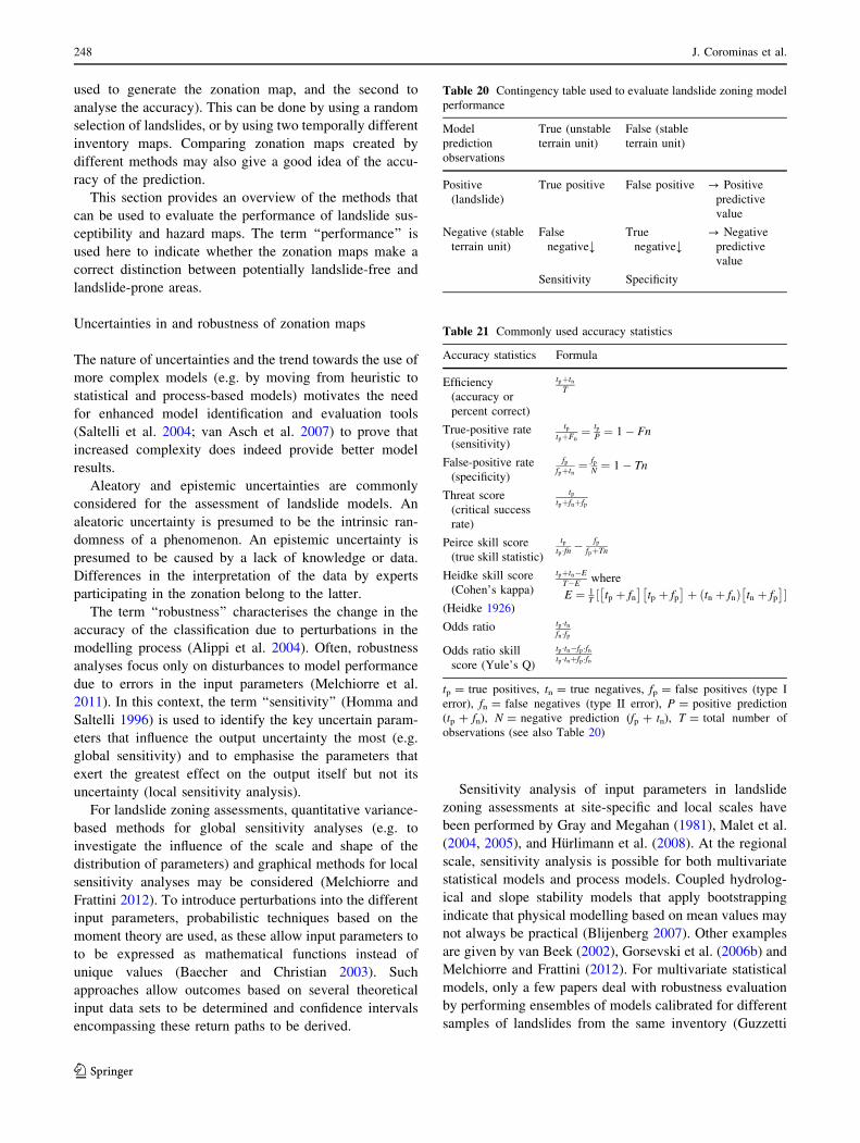
used to generate the zonation map, and the second to

analyse the accuracy). This can be done by using a random

selection of landslides, or by using two temporally different

inventory maps. Comparing zonation maps created by

different methods may also give a good idea of the accu-

racy of the prediction.

This section provides an overview of the methods that

can be used to evaluate the performance of landslide sus-

ceptibility and hazard maps. The term ‘‘performance’’ is

used here to indicate whether the zonation maps make a

correct distinction between potentially landslide-free and

landslide-prone areas.

Uncertainties in and robustness of zonation maps

The nature of uncertainties and the trend towards the use of

more complex models (e.g. by moving from heuristic to

statistical and process-based models) motivates the need

for enhanced model identification and evaluation tools

(Saltelli et al. 2004; van Asch et al. 2007) to prove that

increased complexity does indeed provide better model

results.

Aleatory and epistemic uncertainties are commonly

considered for the assessment of landslide models. An

aleatoric uncertainty is presumed to be the intrinsic ran-

domness of a phenomenon. An epistemic uncertainty is

presumed to be caused by a lack of knowledge or data.

Differences in the interpretation of the data by experts

participating in the zonation belong to the latter.

The term ‘‘robustness’’ characterises the change in the

accuracy of the classification due to perturbations in the

modelling process (Alippi et al. 2004). Often, robustness

analyses focus only on disturbances to model performance

due to errors in the input parameters (Melchiorre et al.

2011). In this context, the term ‘‘sensitivity’’ (Homma and

Saltelli 1996) is used to identify the key uncertain param-

eters that influence the output uncertainty the most (e.g.

global sensitivity) and to emphasise the parameters that

exert the greatest effect on the output itself but not its

uncertainty (local sensitivity analysis).

For landslide zoning assessments, quantitative variance-

based methods for global sensitivity analyses (e.g. to

investigate the influence of the scale and shape of the

distribution of parameters) and graphical methods for local

sensitivity analyses may be considered (Melchiorre and

Frattini 2012). To introduce perturbations into the different

input parameters, probabilistic techniques based on the

moment theory are used, as these allow input parameters to

to be expressed as mathematical functions instead of

unique values (Baecher and Christian 2003). Such

approaches allow outcomes based on several theoretical

input data sets to be determined and confidence intervals

encompassing these return paths to be derived.

Sensitivity analysis of input parameters in landslide

zoning assessments at site-specific and local scales have

been performed by Gray and Megahan (1981), Malet et al.

(2004, 2005), and Hurlimann et al. (2008). At the regional

scale, sensitivity analysis is possible for both multivariate

statistical models and process models. Coupled hydrolog-

ical and slope stability models that apply bootstrapping

indicate that physical modelling based on mean values may

not always be practical (Blijenberg 2007). Other examples

are given by van Beek (2002), Gorsevski et al. (2006b) and

Melchiorre and Frattini (2012). For multivariate statistical

models, only a few papers deal with robustness evaluation

by performing ensembles of models calibrated for different

samples of landslides from the same inventory (Guzzetti

Table 20 Contingency table used to evaluate landslide zoning model

performance

Model

prediction

observations

True (unstable

terrain unit)

False (stable

terrain unit)

Positive

(landslide)

True positive False positive ? Positive

predictive

value

Negative (stable

terrain unit)

False

negative;True

negative;? Negative

predictive

value

Sensitivity Specificity

Table 21 Commonly used accuracy statistics

Accuracy statistics Formula

Efficiency

(accuracy or

percent correct)

tpþtn

T

True-positive rate

(sensitivity)

tptpþFn

¼ tpP¼ 1� Fn

False-positive rate

(specificity)

fp

fpþtn¼ fp

N¼ 1� Tn

Threat score

(critical success

rate)

tp

tpþfnþfp

Peirce skill score

(true skill statistic)

tp

tp �fn�fp

fpþTn

Heidke skill score

(Cohen’s kappa)

(Heidke 1926)

tpþtn�E

T�Ewhere

E ¼ 1T½ tp þ fn� �

tp þ fp� �

þ tn þ fnð Þ tn þ fp� �

�

Odds ratio tp �tn

fn �fp

Odds ratio skill

score (Yule’s Q)

tp �tn�fp �fn

tp �tnþfp �fn

tp = true positives, tn = true negatives, fp = false positives (type I

error), fn = false negatives (type II error), P = positive prediction

(tp ? fn), N = negative prediction (fp ? tn), T = total number of

observations (see also Table 20)


123

et al. 2006; Van Den Eeckhaut et al. 2009; Rossi et al.

2010) or by calibrating models for different landslide

inventories of the same region (Blahut et al. 2010b). A few

studies have investigated the impact of, for example, dif-

ferent classifications of the independent variables derived

from lithological, soil or land-cover maps (Thiery et al.

2007). For instance, Melchiorre et al. (2011) defined a

robustness index showing sensitivity to variations in the

data set of independent (predictor) variables.

Accuracy of the zonation maps

None of the techniques presented in the literature to assess

the accuracy of landslide zoning models account for the

economic costs of misclassification, which become

important when landslide zoning is adopted in practice for

land planning. This is a significant limitation on landslide

susceptibility analysis, as the costs of misclassification vary

depending on the type of error:

• A type I error (false positive) means that a unit without

landslides is classified as unstable, and therefore limited

in its use and economic development. Hence, the false-

positive misclassification cost represents the loss of

economic value of these terrain units. This cost differs

for each terrain unit as it is a function of environmental

and socio-economic characteristics.

• A type II error (false negative) means that a terrain unit

with landslides is classified as stable, and can conse-

quently be used without restrictions. The false negative

misclassification cost is equal to the loss of elements at

risk that can be impacted by landslides in these units.

In landslide zoning models, costs relating to type II

errors are normally much larger than those relating to type I

errors. For example, siting a public facility such as a school

building in a terrain unit that is incorrectly identified as

stable (type II error) could lead to very large social and

economic costs.

In the following, different techniques for the evaluation

of landslide model performance are presented.

Cutoff-dependent accuracy statistics

The accuracy is assessed by analysing the agreement

between the model outputs and the observations. Since the

observed data comprise the presence/absence of landslides

within a certain terrain unit, a simpler method of assessing

the accuracy is to compare these data with a binary clas-

sification of susceptibility into stable and unstable units.

This classification requires a cutoff value in susceptibility

that divides terrains into stable (which have a susceptibility

less than the cutoff) and unstable (which have a suscepti-

bility greater than the cutoff). A comparison of the

observed data and model results after they have been

reclassified into these two classes is represented using

contingency tables (Table 20). Accuracy statistics assess

model performance by combining correctly and incorrectly

classified positives (e.g. unstable areas) and negatives (e.g.

stable areas) (Table 21).

The efficiency, which measures the percentage of

observations that are correctly classified by the model, is

unreliable because it is heavily influenced by the most

common class, usually ‘‘stable terrain unit’’, and it is not

equitable (e.g. it gives the same score for different types of

unskilled classifications), and this must be taken into

account. The true-positive (TP) rate and the false-positive

(FP) rate are insufficient performance statistics because

they ignore false positives and false negatives, respec-

tively. They are not equitable, and they are useful only

when used in conjunction (such as in ROC curves). The

threat score (Gilbert 1884) measures the fraction of

observed and/or classified events that were correctly pre-

dicted. Because it penalises both false negatives and false

positives, it does not distinguish the source of classification

error. Moreover, it depends on the event frequency (and

thus poorer accuracy scores are derived for rarer, i.e. usu-

ally larger-in-magnitude, events), since some true positives

can occur purely due to random chance. Alternatively,

Peirce’s skills score (Peirce 1884) or the odds ratio (Ste-

phenson 2000) may be used.

Accuracy statistics require the division of the classified

objects into a few classes by defining specific values of the

susceptibility index that are called cutoff values. For sta-

tistical models, there is a statistically significant probability

cutoff (p[cutoff]) that is equal to 0.5. When the groups of

stable and unstable terrain units are equal in size and they

approximate a normal distribution, this value maximises

the number of correctly predicted stable and unstable units.

However, the cutoff value used to define the susceptibility

classes is chosen arbitrarily and, unless a cost criterion is

adopted (Provost and Fawcett 1997), depends on the

objective of the map, the number of classes and the type of

modelling approach employed.

A first solution to this limitation consists of evaluating

model performance over a large range of cutoff values

using cutoff-independent performance criteria. Another

option consists of finding the optimal cutoff by minimising

the costs.

Cutoff-independent accuracy statistics: ROC curves

and SR curves

The most commonly used cutoff-independent performance

techniques for landslide zoning models are receiver oper-

ating characteristic (ROC) curves and success-rate curves

(SR).


123

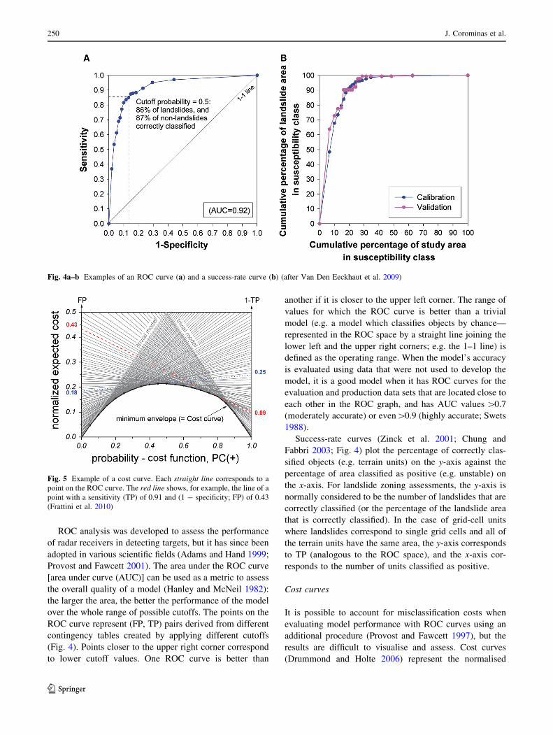
ROC analysis was developed to assess the performance

of radar receivers in detecting targets, but it has since been

adopted in various scientific fields (Adams and Hand 1999;

Provost and Fawcett 2001). The area under the ROC curve

[area under curve (AUC)] can be used as a metric to assess

the overall quality of a model (Hanley and McNeil 1982):

the larger the area, the better the performance of the model

over the whole range of possible cutoffs. The points on the

ROC curve represent (FP, TP) pairs derived from different

contingency tables created by applying different cutoffs

(Fig. 4). Points closer to the upper right corner correspond

to lower cutoff values. One ROC curve is better than

another if it is closer to the upper left corner. The range of

values for which the ROC curve is better than a trivial

model (e.g. a model which classifies objects by chance—

represented in the ROC space by a straight line joining the

lower left and the upper right corners; e.g. the 1–1 line) is

defined as the operating range. When the model’s accuracy

is evaluated using data that were not used to develop the

model, it is a good model when it has ROC curves for the

evaluation and production data sets that are located close to

each other in the ROC graph, and has AUC values [0.7

(moderately accurate) or even[0.9 (highly accurate; Swets

1988).

Success-rate curves (Zinck et al. 2001; Chung and

Fabbri 2003; Fig. 4) plot the percentage of correctly clas-

sified objects (e.g. terrain units) on the y-axis against the

percentage of area classified as positive (e.g. unstable) on

the x-axis. For landslide zoning assessments, the y-axis is

normally considered to be the number of landslides that are

correctly classified (or the percentage of the landslide area

that is correctly classified). In the case of grid-cell units

where landslides correspond to single grid cells and all of

the terrain units have the same area, the y-axis corresponds

to TP (analogous to the ROC space), and the x-axis cor-

responds to the number of units classified as positive.

Cost curves

It is possible to account for misclassification costs when

evaluating model performance with ROC curves using an

additional procedure (Provost and Fawcett 1997), but the

results are difficult to visualise and assess. Cost curves

(Drummond and Holte 2006) represent the normalised

Fig. 4a–b Examples of an ROC curve (a) and a success-rate curve (b) (after Van Den Eeckhaut et al. 2009)

Fig. 5 Example of a cost curve. Each straight line corresponds to a

point on the ROC curve. The red line shows, for example, the line of a

point with a sensitivity (TP) of 0.91 and (1 - specificity; FP) of 0.43

(Frattini et al. 2010)


123

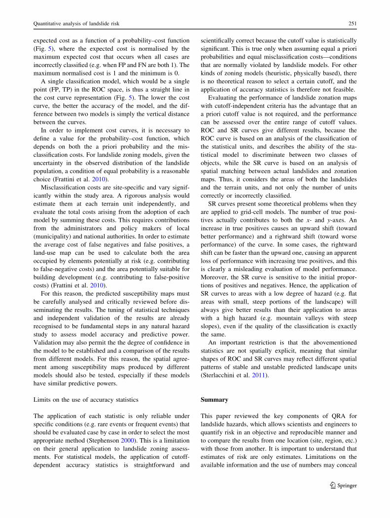
expected cost as a function of a probability–cost function

(Fig. 5), where the expected cost is normalised by the

maximum expected cost that occurs when all cases are

incorrectly classified (e.g. when FP and FN are both 1). The

maximum normalised cost is 1 and the minimum is 0.

A single classification model, which would be a single

point (FP, TP) in the ROC space, is thus a straight line in

the cost curve representation (Fig. 5). The lower the cost

curve, the better the accuracy of the model, and the dif-

ference between two models is simply the vertical distance

between the curves.

In order to implement cost curves, it is necessary to

define a value for the probability–cost function, which

depends on both the a priori probability and the mis-

classification costs. For landslide zoning models, given the

uncertainty in the observed distribution of the landslide

population, a condition of equal probability is a reasonable

choice (Frattini et al. 2010).

Misclassification costs are site-specific and vary signif-

icantly within the study area. A rigorous analysis would

estimate them at each terrain unit independently, and

evaluate the total costs arising from the adoption of each

model by summing these costs. This requires contributions

from the administrators and policy makers of local

(municipality) and national authorities. In order to estimate

the average cost of false negatives and false positives, a

land-use map can be used to calculate both the area

occupied by elements potentially at risk (e.g. contributing

to false-negative costs) and the area potentially suitable for

building development (e.g. contributing to false-positive

costs) (Frattini et al. 2010).

For this reason, the predicted susceptibility maps must

be carefully analysed and critically reviewed before dis-

seminating the results. The tuning of statistical techniques

and independent validation of the results are already

recognised to be fundamental steps in any natural hazard

study to assess model accuracy and predictive power.

Validation may also permit the the degree of confidence in

the model to be established and a comparison of the results

from different models. For this reason, the spatial agree-

ment among susceptibility maps produced by different

models should also be tested, especially if these models

have similar predictive powers.

Limits on the use of accuracy statistics

The application of each statistic is only reliable under

specific conditions (e.g. rare events or frequent events) that

should be evaluated case by case in order to select the most

appropriate method (Stephenson 2000). This is a limitation

on their general application to landslide zoning assess-

ments. For statistical models, the application of cutoff-

dependent accuracy statistics is straightforward and

scientifically correct because the cutoff value is statistically

significant. This is true only when assuming equal a priori

probabilities and equal misclassification costs—conditions

that are normally violated by landslide models. For other

kinds of zoning models (heuristic, physically based), there

is no theoretical reason to select a certain cutoff, and the

application of accuracy statistics is therefore not feasible.

Evaluating the performance of landslide zonation maps

with cutoff-independent criteria has the advantage that an

a priori cutoff value is not required, and the performance

can be assessed over the entire range of cutoff values.

ROC and SR curves give different results, because the

ROC curve is based on an analysis of the classification of

the statistical units, and describes the ability of the sta-

tistical model to discriminate between two classes of

objects, while the SR curve is based on an analysis of

spatial matching between actual landslides and zonation

maps. Thus, it considers the areas of both the landslides

and the terrain units, and not only the number of units

correctly or incorrectly classified.

SR curves present some theoretical problems when they

are applied to grid-cell models. The number of true posi-

tives actually contributes to both the x- and y-axes. An

increase in true positives causes an upward shift (toward

better performance) and a rightward shift (toward worse

performance) of the curve. In some cases, the rightward

shift can be faster than the upward one, causing an apparent

loss of performance with increasing true positives, and this

is clearly a misleading evaluation of model performance.

Moreover, the SR curve is sensitive to the initial propor-

tions of positives and negatives. Hence, the application of

SR curves to areas with a low degree of hazard (e.g. flat

areas with small, steep portions of the landscape) will

always give better results than their application to areas

with a high hazard (e.g. mountain valleys with steep

slopes), even if the quality of the classification is exactly

the same.

An important restriction is that the abovementioned

statistics are not spatially explicit, meaning that similar

shapes of ROC and SR curves may reflect different spatial

patterns of stable and unstable predicted landscape units

(Sterlacchini et al. 2011).

Summary

This paper reviewed the key components of QRA for

landslide hazards, which allows scientists and engineers to

quantify risk in an objective and reproducible manner and

to compare the results from one location (site, region, etc.)

with those from another. It is important to understand that

estimates of risk are only estimates. Limitations on the

available information and the use of numbers may conceal


123

potentially significant errors. In that respect, QRA is not

necessarily more accurate than qualitative estimations as,

for example, probability may be calculated based on per-

sonal judgement. However, QRA facilitates communica-

tion between geoscience professionals, land owners and

decision makers.

Recommended methodologies for the quantitative ana-

lysis of the landslide hazard, vulnerability and risk at dif-

ferent scales (site-specific, local, regional and national)

have been presented, as well as verification and validation

methods.

The methodologies described here focus on the evalu-

ation of the probabilities of occurrence of different land-

slide types with certain characteristics. Methods to

determine the spatial distribution of landslide intensity, the

characterisation of the elements at risk, the assessment of

the potential degree of damage and the quantification of the

vulnerability of the elements at risk, as well as the QRA,

are also described.

The paper is intended for use by scientists and practising

engineers, geologists and other landslide experts.

Acknowledgments The authors are grateful for the support of the

SafeLand project (grant agreement 226479) funded by the European

Commission within its Seventh Framework Programme.

Open Access This article is distributed under the terms of the

Creative Commons Attribution License which permits any use, dis-

tribution, and reproduction in any medium, provided the original

author(s) and the source are credited.

Appendix: Definitions and terminology

Most of the terms used in this document are consistent with

landslide hazard and risk definitions proposed by interna-

tional committees such as Fell et al. (2008a), TC32 (2004)

and UN-ISDR (2004).

Consequence The outcomes or potential outcomes aris-

ing from the occurrence of a landslide, expressed qualita-

tively or quantitatively in terms of loss, disadvantage or

gain; damage, injury or loss of life.

Danger The natural phenomenon that could lead to

damage, described in terms of its geometry and mechanical

and other characteristics. The danger can be an existing one

(such as a creeping slope) or a potential one (such as a rock

fall). The characterisation of a danger does not include any

forecasting.

Elements at risk The population, buildings and engi-

neering structures, economic activities, public services,

utilities, infrastructure, cultural and environmental features

in the area potentially affected by landslides.

Exposure The presence of people, structures, property,

systems, or other elements in zones that may be impacted

by landslides.

Frequency A measure of likelihood expressed as the

number of occurrences of an event in a given time. See also

‘‘likelihood’’ and ‘‘probability’’.

Hazard A condition with the potential for causing an

undesirable consequence. The characterisation of landslide

hazard should include the location, volume (or area),

classification and velocity of the potential landslides and

any resultant detached material, and the probability of their

occurrence within a given period of time.

Hazard zoning The subdivision of the terrain into zones

that are characterised by the temporal probability of

occurrence of landslides of a particular intensity within a

given period of time. Landslide hazard maps should indi-

cate the zones where landslides may occur as well as the

runout zones.

Individual risk to life The risk of fatality or injury to any

identifiable individual who is within the zone impacted by

the landslide, or who follows a particular pattern of life that

might subject him or her to the consequences of the

landslide.

Landslide inventory A record of recognised landslides

in a particular area combined with attribute information.

These attributes should ideally contain information on the

type of landslide, date of occurrence or relative age, size

and/or volume, current activity, and causes. Landslide

inventories are either continuous in time, or provide so-

called event-based landslide inventories, which are inven-

tories of landslides that happened as a result of a particular

triggering event (rainfall, earthquake).

Landslide activity The stage of development of a land-

slide; pre-failure, when the slope is strained throughout but

is essentially intact; failure, characterised by the formation

of a continuous surface of rupture; post-failure, which

includes movement from just after failure to when it

essentially stops; and reactivation, when the slope slides

along one or several pre-existing surfaces of rupture.

Reactivation may be occasional (e.g. seasonal) or contin-

uous (in which case the slide is ‘‘active’’).

Landslide hazard assessment The estimation of the

zones where landslides of a particular type, volume, runout

and intensity may occur within a given period of time.

Landslide hazard map A map showing the subdivision

of the terrain into zones that are characterised by the

probability of occurrence of landslides of a particular

intensity. Landslide hazard maps should indicate the zones

where landslides may occur as well as the runout zones.


123

Landslide intensity A set of spatially distributed

parameters related to the destructive power of a landslide.

The parameters may be described quantitatively or quali-

tatively, and may include maximum movement velocity,

total displacement, differential displacement, depth of the

moving mass, peak discharge per unit width or kinetic

energy per unit area.

Landslide magnitude The measure of the landslide size.

It may be quantitatively described by its volume or (indi-

rectly) by its area. The latter descriptors may refer to the

landslide scar, the landslide deposit, or both.

Landslide probability In the framework of landslide

hazard, the following types of probability are important:

• Spatial probability: the probability that a given area is

hit by a landslide

• Temporal probability: the probability that a given

triggering event will cause landslides

• Size/volume probability: the probability that the slide

has a given size/volume

• Reach probability: the probability that the slide will

travel a certain distance downslope.

Landslide risk map A map showing the subdivision of

the terrain into zones that are characterised by different

probabilities of losses that might occur due to landslides of

a given type within a given period of time. It is usually

calculated as

• The expected losses in a particular area struck by a

landslide of a given magnitude (intensity) in a given

year,

• A recurrence interval, i.e. the expected losses in a

particular area struck by the 100-year landslide event,

or

• The cumulative losses during a given time interval due

to landslides with different return periods.

Landslide susceptibility assessment A quantitative or

qualitative assessment of the classifications, volumes (or

areas) and spatial distribution of landslides which exist or

potentially may occur in an area.

Landslide susceptibility map A map showing the sub-

division of the terrain into zones that have a different

likelihood of a landslide of a given type occurring. It

should indicate the zones where landslides may occur as

well as the runout zones.

Likelihood Used as a qualitative description of proba-

bility or frequency.

Population at risk All of the people who would be

directly exposed to the consequences of landslides.

Probability A measure of the degree of certainty. This

measure has a value between zero (impossibility) and 1.0

(certainty). It is an estimate of the likelihood of the mag-

nitude of the uncertain quantity, or the likelihood of the

occurrence of the uncertain future event.

Qualitative risk analysis An analysis which uses word-

form, descriptive or numerical scales to describe the

magnitude of potential consequences and the likelihood

that those consequences will occur.

Quantitative risk analysis An analysis based on

numerical values of the probability, vulnerability and con-

sequences, and resulting in a numerical value of the risk.

Recurrence interval The long-term average elapsed

time between landslide events at a particular site or in a

specified area. Also known as ‘‘return period’’.

Reach probability/runout probability The probability

that a specified landslide will reach a certain distance.

Residual risk The degree of risk that exists given the

presence of risk-mitigation measures.

Risk A measure of the probability and severity of an

adverse effect to health, property or the environment. Risk

is often defined as the probability of the landslide event

multiplied by the consequences.

Risk analysis The use of available information to cal-

culate the risk to individuals, population, property or the

environment from hazards. Risk analyses generally contain

the following steps: scope definition, hazard identification,

vulnerability evaluation and risk estimation.

Risk assessment The process of making a recommen-

dation on whether existing risks are acceptable and present

risk control measures are adequate, and if they are not,

whether alternative risk control measures are justified or

will be implemented. Risk assessment incorporates the risk

analysis and risk evaluation phases.

Risk control/risk treatment The process of decision

making for managing risk, and the implementation or

enforcement of risk mitigation measures and the re-evalu-

ation of its effectiveness from time to time, using the

results of risk assessment as one input.

Risk evaluation The stage at which values and judge-

ments enter the decision process, explicitly or implicitly,

including consideration of the importance of the estimated

risks and the associated social, environmental and eco-

nomic consequences, in order to identify a range of alter-

natives for managing the risks.

Risk management The complete process of risk assess-

ment and risk control.


123

Societal risk The risk of multiple fatalities, injuries, or

disruption of activities in society as a whole: one where

society would have to carry the burden of a landslide

causing a number of deaths, injuries, financial, environ-

mental, and other losses.

Spatiotemporal probability of the element at risk The

probability that the element at risk is in the path of the

landslide at the time of its occurrence. It is the quantitative

expression of the exposure.

Validation The process of determining the degree to

which a model is an accurate representation of the real

world from the perspective of the intended uses of the

model.

Verification The process of determining that the imple-

mentation of the model accurately represents the devel-

oper’s conceptual description of the model and its solution.

Vulnerability The degree of loss of a given element or

set of elements exposed to the occurrence of a landslide of

a given magnitude/intensity. It is expressed on a scale of 0

(no loss) to 1 (total loss).

Zoning The act of dividing land into homogeneous areas

or domains and then ranking them according to degrees of

actual or potential landslide susceptibility, hazard or risk.

It is important that those carrying out landslide mapping

use consistent terminology to classify and characterise

landslides. It is recommended that the classification and

terminology are based on well-known schemes such as

Cruden and Varnes (1996), Hungr et al. (2001, 2012), and

IAEG (1990).

References

Abbruzzese JM, Sauthier C, Labiouse V (2009) Considerations on

Swiss methodologies for rock fall hazard mapping based on

trajectory modelling. Nat Hazards Earth Syst Sci 9:1095–1109

Adams NM, Hand DJ (1999) Comparing classifiers when the

misallocations costs are uncertain. Pattern Recogn 32:

1139–1147

Agliardi F, Crosta GB (2003) High resolution three-dimensional

numerical modelling of rockfalls. Int J Rock Mech Min Sci

40:455–471

Agliardi F, Crosta GB, Zanchi A, Ravazzi C (2009a) Onset and

timing of deep-seated gravitational slope deformations in the

eastern Alps, Italy. Geomorphology 103:113–129

Agliardi F, Crosta GB, Frattini P (2009b) Integrating rockfall risk

assessment and countermeasure design by 3D modelling tech-

niques. Nat Hazards Earth Syst Sci 9:1059–1073

AGS (2000) Landslide risk management concepts and guidelines.

Australian Geomechanics Society. Aust Geomech 35(1):49–92

AGS (2007) Guidelines for landslide susceptibility, hazard and risk

zoning for land use management. Australian Geomechanics

Society Landslide Taskforce Landslide Zoning Working Group.

Aust Geomech 42(1):13–36

Akbas SO, Blahut J, Sterlacchini S (2009) Critical assessment of

existing physical vulnerability estimation approaches for debris

flows. In: Malet JP, Remaitre A, Bogaard T (eds) Proceedings of

landslide processes: from geomorphologic mapping to dynamic

modelling. CERG Editions, Strasburg, pp 229–233

Amatruda G et al (2004) A key approach: the IMIRILAND project

method. In: Bonnard Ch, Forlati F, Scavia C (eds) Identification

and mitigation of large landslides risks in Europe. IMIRILAND

PROJECT—European Commission—Fifth Framework Program.

A.A. Balkema, Amsterdam, pp 13–43

Aleotti P, Chowdhury R (1999) Landslide hazard assessment:

summary review and new perspectives. Bull Eng Geol Environ

58:21–44

Alexander ED (2005) Vulnerability to landslides. In: Glade T,

Anderson MG, Crozier MJ (eds) Landslide risk assessment.

Wiley, London, pp 175–198

Alippi C, Sana D, Scotti F (2004) A training-time analysis of

robustness in feed-forward neural networks. In: Proceedings of

the International Joint Conference on Neural Networks

IJCNN04, Budapest, Hungary. IEEE, New York, pp 2853–2858

Alonso EE, Pinyol NM (2010) Criteria for rapid sliding I: a review of

the Vaiont case. Eng Geol 114:198–210

Archetti R, Lamberti A (2003) Assessment of risk due to debris flow

events. Nat Hazards Rev 4(3):115–125

Ardizzone F, Cardinali M, Carrara A, Guzzetti F, Reichenbach P

(2002) Impact of mapping errors on the reliability of landslide

hazard maps. Nat Hazards Earth Syst Sci 2:3–14

Ardizzone F, Cardinali M, Galli M, Guzzetti F, Reichenbach P (2007)

Identification and mapping of recent rainfall-induced landslides

using elevation data collected by airborne Lidar. Nat Hazards

Earth Syst Sci 7:637–650

Asselen SV, Seijmonsbergen AC (2006) Expert-driven semi-auto-

mated geomorphological mapping for a mountainous area using

a laser DTM. Geomorphology 78(3–4):309–320

ATC (1985) ATC-13: Earthquake damage evaluation data for

California. Applied Technology Council, Redwood City

Ayala FJ, Cubillo S, Alvarez A, Domınguez MJ, Laın L, Laın R, Ortız

G (2003) Large scale rockfall reach susceptibility maps in La

Cabrera Sierra (Madrid) performed with GIS and dynamic

analysis at 1:5,000. Nat Hazards 30:325–340

Azzoni A, La Barbera G, Zaninetti A (1995) Analysis and prediction

of rock falls using a mathematical model. Int J Rock Mech Min

Sci Geomech Abstr 32:709–724

Baecher GB, Christian JT (2003) Reliability and statistics in

geotechnical engineering. Wiley, New York

Bakker MM, Govers G, Kosmas C, Vanacker V, van Oost K,

Rounsevell M (2005) Soil erosion as a driver of land-use change.

Agric Ecosyst Environ 105(3):467–481

Bathurst JC, Moretti G, El-Hames A, Begueria S, Garcia-Ruiz JM

(2007) Modelling the impact of forest loss on shallow landslide

sediment yield, Ijuez river catchment, Spanish Pyrenees. Hydrol

Earth Syst Sci 11(1):569–583

Baum RL, Godt JW (2010) Early warning of rainfall-induced shallow

landslides and debris flows in the USA. Landslides 7:259–272

Baum RL, Savage WZ, Godt JW (2002) TRIGRS—a FORTRAN

program for transient rainfall infiltration and grid-based regional

slope stability analysis. US Geological Survey Open-File Report

02-0424. Available via http://pubs.usgs.gov/of/2002/ofr-02-424/

Baum R, Coe JA, Godt JW, Harp EL, Reid ME, Savage WZ, Schulz

WH, Brien DL, Chleborad AF, McKenna JP, Michael JA (2005)

Regional landslide-hazard assessment for Seattle, Washington,

USA. Landslides 2:266–279

Begueria S (2006) Validation and evaluation of predictive models in

hazard assessment and risk management. Nat Hazards 37(3):

315–329


123

http://pubs.usgs.gov/of/2002/ofr-02-424/

Bell R, Glade T (2004) Quantitative risk analysis for landslides—

examples from Bıldudalur, NW-Iceland. Nat Hazard Earth Syst

Sci 4(1):117–131

Berardino P, Fornaro G, Lanari R, Sansosti E (2002) A new algorithm

for surface deformation monitoring based on small baseline

differential interferograms. IEEE Trans Geosci Remote Sens

40(11):2375–2383

Berti M, Simoni A (2007) Prediction of debris flow inundation areas

using empirical mobility relationships. Geomorphology 90:144–

161

Bird JF, Bommer JJ, Crowley H, Pinho R (2006) Modelling

liquefaction-induced building damage in earthquake loss esti-

mation. Soil Dyn Earthq Eng 26(1):15–30

Blahut J, Horton P, Sterlacchini S, Jaboyedoff M (2010a) Debris flow

hazard modelling on medium scale: Valtellina di Tirano, Italy.

Nat Hazards Earth Syst Sci 10:2379–2390

Blahut J, van Westen CJ, Sterlacchini S (2010b) Analysis of landslide

inventories for accurate prediction of debris-flow source areas.

Geomorphology 119(1–2):36–51

Blijenberg HM (2007) Application of physical modelling of debris

flow triggering to field conditions: limitations posed by boundary

conditions. Eng Geol 91(1):25–33

Bonham-Carter GF (1994) Geographic information system for

geoscientists: modelling with GIS. Pergamon, Oxford, p 398

Borghuis AM, Chang K, Lee HY (2007) Comparison between

automated and manual mapping of typhoon-triggered landslides

from SPOT-5 imagery. Int J Remote Sens 28:1843–1856

Borter P (1999) Risikoanalyse bei gravitativen Naturgefahren.

Bundesamt fur Umwelt, Wald und Landschaft, Bern

Bovolin V, Taglialatela L (2002) Proceedings Scritti in onore di

Lucio Taglialatela. CNR-GNDCI publ. no. 2811. CNR-GNDCI,

Perugia, pp 429–437

Bozzolo D, Pamini R (1986) Simulation of rock falls down a valley

side. Acta Mech 63:113–130

Brabb EE (1984) Innovative approaches to landslide hazard mapping.

In: 4th Int Symp on Landslides, Toronto, Canada, 16–21 Sept

1984, 1:307–324

Brabb EE, Pampeyan EH, Bonilla MG (1972) Landslide susceptibility

in San Mateo County, California. Misc. Field Studies, map MF-

360 (scale 1:62,500). US Geological Survey, Reston

Brand EW (1988) Special lecture: landslide risk assessment in Hong

Kong. In: Proceedings of the V International Symposium on

Landslides, Lausanne, Switzerland. A.A. Balkema, Amsterdam,

2:1059–1074

Brardinoni F, Church M (2004) Representing the landslide magni-

tude–frequency relation, Capilano River Basin, British Colum-

bia. Earth Surf Proc Land 29:115–124

Brenner C (2005) Building reconstruction from images and laser

scanning. Int J Appl Earth Obs Geoinf 6(3–4):187–198

Brunetti MT, Guzzetti F, Rossi M (2009) Probability distributions of

landslide volumes. Nonlinear Process Geophys 16:179–188

Budetta PB (2002) Risk assessment from debris flows in pyroclastic

deposits along a motorway, Italy. Bull Eng Geol Environ

61(4):293–301

Bull WB, Brandon MT (1998) Lichen dating of earthquake-generated

regional rockfall events, Southern Alps, New Zealand. GSA Bull

110:60–84

Bull WB, King J, Kong F, Moutoux T, Philips WM (1994) Lichen

dating of coseismic landslide hazards in alpine mountains.

Geomorphology 10:253–264

Bulut F, Boynukalin S, Tarhan F, Ataoglu E (2000) Reliability of

isopleth maps. Bull Eng Geol Environ 58:95–98

Bunce CM, Cruden DM, Morgenstern NR (1997) Assessment of the

hazard from rock fall on a highway. Can Geotech J 34:344–356

Calvetti F, Crosta G, Tatarella M (2000) Numerical simulation of dry

granular flows: from the reproduction of small-scale experiments

to the prediction of rock avalanches. Rivista Italiana di

Geotecnica 2000:21–38

Calvo B, Savi F (2009) A real-world application of Monte Carlo

procedure for debris flow risk assessment. Comput Geosci

35(5):967–977

Cardinali M (2002) A geomorphological approach to the estimation

of landslide hazards and risk in Umbria, Central Italy. Nat

Hazards Earth Syst Sci 2:57–72

Carrara A (1983) Multivariate models for landslide hazard evolution.

Math Geol 15:403–427

Carrara A, Guzzetti F, Cardinali M, Reichenbach P (1999) Use of GIS

technology in the prediction and monitoring of landslide hazard.

Nat Hazards 20(2–3):117–135

Casadei M, Dietrich WE, Mille NL (2003) Testing a model for

predicting the timing and location of shallow landslide initiation

on soil mantled landscapes. Earth Surf Proc Land 28(9):925–950

Cascini L (2008) Applicability of landslide susceptibility and hazard

zoning at different scales. Eng Geol 102:164–177

Cascini L, Bonnard Ch, Corominas J, Jibson R, Montero-Olarte J

(2005) Landslide hazard and risk zoning for urban planning and

development—state of the art report. In: Hungr O, Fell R,

Couture R, Eberhardt E (eds) Landslide risk management. A.A.

Balkema, Amsterdam, pp 199–235

Cascini L, Cuomo S, Ferlisi S, Sorbino G (2009) Detection of

mechanisms for destructive landslides in Campania region—

southern Italy. In: Picarelli L, Tommasi P, Urciuoli G, Versace P

(eds) Proceedings of the Workshop on Rainfall-Induced Land-

slides: Mechanisms, Monitoring Techniques and Nowcasting

Models for Early Warning Systems, vol 1, Naples, 8–10 June

2009. Studio Editoriale Doppiavoce, Napoli, pp 43–51

Catani F, Casagli N, Ermini L, Righini G, Menduni G (2005)

Landslide hazard and risk mapping at catchment scale in the

Arno River basin. Landslides 2:329–342

Catani F, Segoni S, Falorni G (2007) Accurate basin scale soil depth

modelling and its impact on shallow landslides prediction.

European Geosciences Union General Assembly 2007, Vienna,

Austria. Geophys Res Abstr 9(10828)

Cepeda J, Colonnelli S, Meyer NK, Kronholm K (2012) SafeLand

Deliverable D1.5: statistical and empirical models for prediction

of precipitation-induced landslides. Available at http://www.

safeland-fp7.eu/

Chacon J, Irigaray C, Fernandez T, El Hamdouni R (2006)Engineering geology maps: landslides and geographical infor-

mation systems. Bull Eng Geol Environ 65:341–411

Chau KT, Wong RHC, Liu J, Lee CF (2003) Rockfall hazard analysis

for Hong Kong based on rockfall inventory. Rock Mech Rock

Eng 36:383–408

Chen K, McAneney J, Blong R, Leigh R, Hunter L, Magill C (2004)

Defining area at risk and its effect in catastrophe loss estimation:

a dasymetric mapping approach. Appl Geogr 24(2004):97–117

Chung CF, Fabbri AG (1993) Representation of geoscience data for

information integration. J Non-Renew Resour 2(2):122–139

Chung CF, Fabbri AG (2003) Validation of spatial prediction models

for landslide hazard mapping. Nat Hazards 30(3):451–472

Coe JA, Michael JA, Crovelli RA, Savage WA (2000) Preliminary

map showing landslides densities, mean recurrence intervals, and

exceedance probabilities as determined from historic records.

Open-file report 00-303. USGS, Seattle

Colesanti C, Wasowski J (2006) Investigating landslides with space-

borne Synthetic Aperture Radar (SAR) interferometry. Eng Geol

88:173–199

Collison A, Wade J, Griths S, Dehn M (2000) Modelling the impact

of predicted climate change on landslide frequency and magni-

tude in SE England. Eng Geol 55:205–218

Comegna L, Picarelli L, Bucchignani E, Mercogliano, P (2012)

Potential effects of incoming climate changes on the behaviour


123

http://www.safeland-fp7.eu/


of slow active landslides in clay. Landslides (in press).

doi:101007/s10346-012-0339-3

Copons R, Vilaplana JM (2008) Rockfall susceptibility zoning at a

large scale: from geomorphological inventory to preliminary

land use planning. Eng Geol 102:142–151

Copons R, Vilaplana JM, Linares R (2009) Rockfall travel distance

analysis by using empirical models (Sola d’Andorra la Vella,

Central Pyrenees). Nat Hazards Earth Syst Sci 9:2107–2118

Cornell CA, Jalayer F, Hamburger RO, Foutch DA (2002) Probabi-

listic basis for 2000 SAC federal emergency management

agency steel moment frame guidelines. J Struct Eng 128:526–

533

Corominas J, Mavrouli O (2011a) Quantitative risk assessment for

buildings due to rockfalls: some achievements and challenges.

In: Journee de Rencontre sur les Dangers Naturels 2011,

Lausanne, Switzerland, 17–18 Feb 2011 (in press)

Corominas J, Mavrouli O (2011b) Rockfall quantitative risk assess-

ment. In: Lambert S, Nicot F (eds) Rockfall engineering: from

prediction to mitigation. Wiley, New York, pp 255–296

Corominas J et al (eds) (2010) SafeLand Deliverable D2.1: overview

of landslide hazard and risk assessment practices. Available at


Corominas J, Moya J (2008) A review of assessing landslide

frequency for hazard zoning purposes. Eng Geol 102:193–213

Corominas J, Moya J (2010) Contribution of dendrochronology to the

determination of magnitude–frequency relationships for land-

slides. Geomorphology 124:137–149. doi:101016/jgeomorph

201009001

Corominas J, Copons R, Vilaplana JM, Altimir J, Amigo J (2003)

Integrated landslide susceptibility analysis and hazard assess-

ment in the principality of Andorra. Nat Hazards 30:421–435

Corominas J, Copons R, Moya J, Vilaplana JM, Altimir J, Amigo J

(2005) Quantitative assessment of the residual risk in a rockfall

protected area. Landslides 2:343–357

Cozzani V, Zanelli S (2001) An approach to the assessment of

domino accidents hazard in quantitative area risk analysis. In:

Pasman HJ, Fredholm O, Jacobsson A (eds) Loss prevention and

safety promotion in the process industries. Elsevier, Amsterdam,

pp 1263–1274

Crosta GB, Agliardi F (2003) A methodology for physically-based

rockfall hazard assessment. Nat Hazards Earth Syst Sci

3:407–422

Crosta GB, Frattini P (2003) Distributed modelling of shallow

landslides triggered by intense rainfall. Nat Hazards Earth Syst

Sci 3(1–2):81–93

Crosta GB, Cucchiaro S, Frattini P (2003) Validation of semi-

empirical relationships for the definition of debris-flow behav-

iour in granular materials. In: Rickenmann D, Chen C (eds)

Proceedings of the Third International Conference on Debris-

Flow Hazards Mitigation: Mechanics, Prediction and Assess-

ment, Davos, Switzerland. Millpress, Rotterdam, pp 821–831

Crosta GB, Agliardi F, Frattini P, Imposimato S (2004) A three-

dimensional hybrid numerical model for rockfall simulation.

Geophys Res Abstr 6:04502

Crosta GB, Imposimato S, Roddeman DG (2008) Numerical model-

ling of entrainment/deposition in rock and debris-avalanches.

Eng Geol 109(1–2):135–145

Crosta GB, Agliardi F, Frattini P, Sosoi R (eds) (2012) SafeLand

Deliverable 1.1: landslide triggering mechanisms in Europe—

overview and state of the art. Identification of mechanisms and

triggers. Available at http://www.safeland-fp7.eu/

Crovelli RA (2000) Probabilistic models for estimation of number and

cost of landslides. Open file report 00-249. US Geological

Survey, Reston, p 23. http://pubs.usgs.gov/of/2002/ofr-02-424/

Crozier MJ (2005) Multiple occurrence regional landslide events in

New Zealand: hazard management issues. Landslides 2:247–256

Crozier MJ, Preston NJ (1999) Modelling changes in terrain

resistance as a component of landform evolution in unstable

hill country. In: Hergarten S, Neugebauer HJ (eds) Process

modelling and landform evolution, lecture notes in earth sciences

78, Springer, Berlin, pp 267–284

Cruden DM, Varnes DJ (1996) Landslide types and processes. In:

Turner AT, Schuster RL (eds) Landslides—investigation and

mitigation. Transportation Research Board Special Report no.

247. National Academy Press, Washington, DC, pp 36–75

Culshaw MG (2005) From concept towards reality: developing the

attributed 3D geological model of the shallow subsurface. Q J

Eng Geol Hydrogeol 38:231–284

Dai FC, Lee CF, Ngai YY (2002) Landslide risk assessment and

management: an overview. Eng Geol 64:65–87

Davis PA, Goodrich MT (1990) A proposed strategy for the

validation of ground-water flow and solute transport models.

Technical report. Sandia National Labs, Albuquerque

Del Gaudio V, Pierri P, Wasowski J (2003) An approach to time-

probabilistic evaluation of seismically induced landslide hazard.

Bull Seismol Soc Am 93(2):557–569

Den Eeckhaut Van, Vanwalleghem T, Poesen J, Govers G, Verstrae-

ten G, Vandekerckhove L (2006) Prediction of landslide

susceptibility using rare events logistic regression: a case-study

in the Flemish Ardennes (Belgium). Geomorphology 76(3–4):

392–410

Den Eeckhaut Van, Reichenbach P, Guzzetti F, Rossi M, Poesen J (2009)

Combined landslide inventory and susceptibility assessment based

on different mapping units: an example from the Flemish Ardennes,

Belgium. Nat Hazards Earth Syst Sci 9:507–521

Dietrich WE, Reiss R, Hsu ML, Montgomery DR (1995) A process-

based model for colluvial soil depth and shallow landsliding

using digital elevation data. Hydrol Process 9:383–400

Dobbs MR, Culshaw MG, Northmore KJ, Reeves HJ, Entwisle DC

(2012) Methodology for creating national engineering geological

maps of the UK. Q J Eng Geol Hydrogeol 45(3):335–347

D’Odorico P (2000) A possible bistable evolution of soil thickness.

J Geophys Res 105(B11):25927–25935

Domaas U (1994) Geometrical methods of calculating rockfall range.

Report 585910-1. Norwegian Geotechnical Institute, Oslo

Dorren LKA, Seijmonsbergen AC (2003) Comparison of three GIS-

based models for predicting rockfall runout zones at a regional

scale. Geomorphology 56:49–64

Drummond C, Holte RC (2006) Cost curves: an improved method for

visualizing classifier performance. Mach Learn 65(1):95–130

Dussauge-Peisser C, Helmstetter A, Grasso J-R, Hantz D, Desvarreux

P, Jeannin M, Giraud A (2002) Probabilistic approach to rock

fall hazard assessment: potential of historical data analysis. Nat

Hazards Earth Syst Sci 2:15–26

Ermini L, Catani F, Casagli N (2005) Artificial neural networks

applied to landslide susceptibility assessment. Geomorphology

66:327–343

Evans SG, Hungr O (1993) The assessment of rockfall hazard at the

base of talus slopes. Can Geotech J 30:620–636

Eveleigh TJ, Mazzucchi TA, Sarkani S (2006) Systems engineering

design and spatial modelling for improved natural hazard risk

assessment. Disaster Prev Manag 15(4):636–648

Eveleigh TJ, Mazzucchi TA, Sarkani S (2007) Spatially-aware

systems engineering design modelling applied to natural hazard

vulnerability assessment. Syst Eng 10(3):187–202

Fannin RJ, Wise MP (2001) An empirical-statistical model for debris

flow travel distance. Can Geotech J 38:982–994

Farina P, Colombo D, Fumagalli A, Marks F, Moretti S (2006)

Permanent scatters for landslide investigations: outcomes from

the ESA-SLAM project. Eng Geol 88:200–217

Farr TG, Rosen PA, Caro E, Crippen R, Duren R, Hensley S, Kobrick

M, Paller M, Rodriguez E, Roth L, Seal D, Shaffer S, Shimada J,


123

http://dx.doi.org/101007/s10346-012-0339-3


http://dx.doi.org/101016/jgeomorph201009001



http://pubs.usgs.gov/of/2002/ofr-02-424/

Umland J, Werner M, Oskin M, Burbank D, Alsdorf D (2007)

The Shuttle Radar Topography Mission. Rev Geophys

45:RG2004. doi:101029/2005RG000183

Fell R, Corominas J, Bonnard Ch, Cascini L, Leroi E, Savage WZ (on

behalf of the JTC-1 Joint Technical Committee on Landslides

and Engineered Slopes) (2008a) Guidelines for landslide

susceptibility, hazard and risk zoning for land use planning.

Eng Geol 102:85–98

Fell R, Corominas J, Bonnard Ch, Cascini L, Leroi E, Savage WZ (on

behalf of the JTC-1 Joint Technical Committee on Landslides

and Engineered Slopes) (2008b) Guidelines for landslide

susceptibility, hazard and risk zoning for land-use planning.

Comment Eng Geol 102:99–111

Fell R, Ho KKS, Lacasse S, Leroi E (2005) A framework for landslide

risk assessment and management. In: Hungr O, Fell R, Couture

R, Eberhardt E (eds) Landslide risk management. Taylor and

Francis, London, pp 3–26

Ferlisi S, Cascini L, Corominas J, Matano F (2012) Rockfall risk

assessment to persons travelling in vehicles along a road: the

case study of the Amalfi coastal road (southern Italy). Nat

Hazards 62(2):691–721

Ferretti A, Prati C, Rocca F (2001) Permanent scatterers in SAR

interferometry. IEEE Trans Geosci Remote Sens 39(1):8–20

Finlay PJ, Fell RA (1996) Study of landslide risk assessment for Hong

Kong. School of Engineering Report. The University of New

South Wales, Sydney

Finlay PJ, Mostyn GR, Fell R (1999) Landslide risk assessment:

prediction of travel distance. Can Geotech J 36:556–562

Fisher PF, Tate NJ (2006) Causes and consequences of error in digital

elevation models. Prog Phys Geogr 30:467

Fotopoulou S, Pitilakis K (2013a) Vulnerability assessment of

reinforced concrete buildings subjected to seismically triggered

slow-moving earth slides. Landslides 10:563–582. doi:101007/

s10346-012-0345-5

Fotopoulou S, Pitilakis K (2013b) Fragility curves for reinforced

concrete buildings to seismically triggered slow-moving slides.

Soil Dyn Earthq Eng 48:143–161

Frattini P, Crosta GB, Sosio R (2009) Approaches for defining

thresholds and return periods for rainfall-triggered shallow

landslides. Hydrol Process 23(10):1444–1460

Frattini P, Crosta GB, Carrara A (2010) Techniques for evaluating the

performance of landslide susceptibility models. Eng Geol

111:62–72

Frattini P, Crosta GB, Lari S, Agliardi F (2012) Probabilistic rockfall

hazard analysis (PRHA). In: Eberhardt E, Froese C, Turner AK,

Leroueil S (eds) Landslides and engineered slopes: protecting

society through improved understanding. Taylor & Francis,

London, pp 1145–1151

Friele P, Jakob M, Clague J (2008) Hazard and risk from large

landslides from Mount Meager Volcano, British Columbia,

Canada. Georisk 2(1):48–64

Fuchs S (2008) Vulnerability to torrent events—empirical evidence

from Austria. Geophys Res Abstr 10:04632. ISSN 1029-7006

Fuchs S, Heiss K, Hubl J (2007) Towards an empirical vulnerability

function for use in debris flow risk assessment. Nat Hazards


Gentile F, Bisantino T, Trisorio Liuzzi G (2008) Debris-flow risk

analysis in south Gargano watersheds (Southern Italy). Nat

Hazards 44:1–17

GEO (2006) Assessment of landslide risk in natural hillsides in Hong

Kong. Report no. 191. Hong Kong Geotechnical Engineering

Office, Hong Kong, p 117

GEO-SLOPE (2011) SLOPE/W. GEO-SLOPE International, Calgary.

http://www.geo-slope.com

Ghosh S, Gunther A, Carranza EJM, van Westen CJ, Jetten VG

(2010) Rock slope instability assessment using spatially

distributed structural orientation data in Darjeeling Himalaya

(India). Earth Surf Proc Land 35(15):1773–1792

Ghosh S, van Westen CJ, Carranza EJ, Jetten VG (2011) Integrating

spatial, temporal, and magnitude probabilities for medium-scale

landslide risk analysis in Darjeeling Himalayas, India. Land-

slides 9:371–384

Gilbert GF (1884) Finley’s tornado predictions. Am Meteorol J

1:166–172

Gitirana Jr G, Santos M, Fredlund M (2008) Three-dimensional slope

stability model using finite element stress analysis. In: GeoCon-

gress 2008, New Orleans, LA, USA, 9–12 March 2008, pp 191–198

Glade T (2003) Landslide occurrence as a response to land use

change: a review of evidence from New Zealand. Catena 51(3–4,

1):297–314

Glade T, Crozier MJ (2005) A review of scale dependency in

landslide hazard and risk analysis. In: Glade T, Anderson M,

Crozier MJ (eds) Landslide hazard and risk. Wiley, London,

pp 75–138

Glade T, Anderson M, Crozier MJ (2005) Landslide hazard and risk.

Wiley, Chichester, p 802

Godt JW, Baum RL, Savage WZ, Salciarini D, Schulz WH, Harp EL

(2008) Transient deterministic shallow landside modelling:

requirements for susceptibility and hazard assessment in a GIS

framework. Eng Geol 102:214–226

Gorsevski PV, Gessler P, Foltz RB (2000) Spatial prediction of

landslide hazard using discriminant analysis and GIS. In: GIS in

the Rockies 2000 Conference and Workshop: Applications for

the 21st Century, Denver, CO, USA, 25–27 Sept 2000

Gorsevski PV, Gessler PE, Foltz RB, Elliot WJ (2006a) Spatial

prediction of landslide hazard using logistic regression and ROC

analysis. Trans GIS 10(3):395–415

Gorsevski PV, Gessler PE, Boll J, Elliot WJ, Foltz RB (2006b)

Spatially and temporally distributed modelling of landslide

susceptibility. Geomorphology 80(3–4):178–198

Gorum T, Fan X, van Westen CJ, Huang RQ, Xu Q, Tang C, Wang G

(2011) Distribution pattern of earthquake-induced landslides

triggered by the 12 May 2008 Wenchuan earthquake. Geomor-

phology 133(3–4):152–167

Govi M, Sorzana PF (1980) Landslide susceptibility as function of

critical rainfall amount in Piedmont basins (North-

Western Italy). Studia Geomorphologica Carpatho-Balcanica

14:43–61

Granger K, Jones T, Leiba M, Scott G (1999) Community risks in

Cairns: a multi-hazard risk assessment. Australian Geological

Survey Organisation, Canberra

Gray DH, Megahan WF (1981) Forest vegetation removal and slope

stability in the Idaho Batholith. Research paper INT-97. USDA,

Washington, DC, p 34

Guimaraes RF, Montgomery DR, Greenberg HM, Fernandes NF,

Trancoso Gomes RA, de Carvalho J, Osmar A (2003) Param-

eterization of soil properties for a model of topographic controls

on shallow landsliding: application to Rio de Janeiro. Eng Geol

69(1–2):99–108

Gunther A (2003) SLOPEMAP: programs for automated mapping of

geometrical and kinematical properties of hard rock hill slopes.

Comput Geosci 29:865–875

Gustavsson M, Kolstrup E, Seijmonsbergen AC (2006) A new

symbol-and-GIS based detailed geomorphological mapping

system: renewal of a scientific discipline for understanding

landscape development. Geomorphology 77(1–2):90–111

Guthrie RH, Evans SG (2004) Analysis of landslide frequencies and

characteristics in a natural system. Coast British Columbia Earth

Surf Process Landf 29:1321–1339

Guthrie RH, Deadman PJ, Raymond Cabrera A, Evans SG (2008)

Exploring the magnitude–frequency distribution: a cellular

automata model for landslides. Landslides 5:151–159


123

http://dx.doi.org/101029/2005RG000183

http://dx.doi.org/101007/s10346-012-0345-5

http://dx.doi.org/101007/s10346-012-0345-5

http://www.geo-slope.com

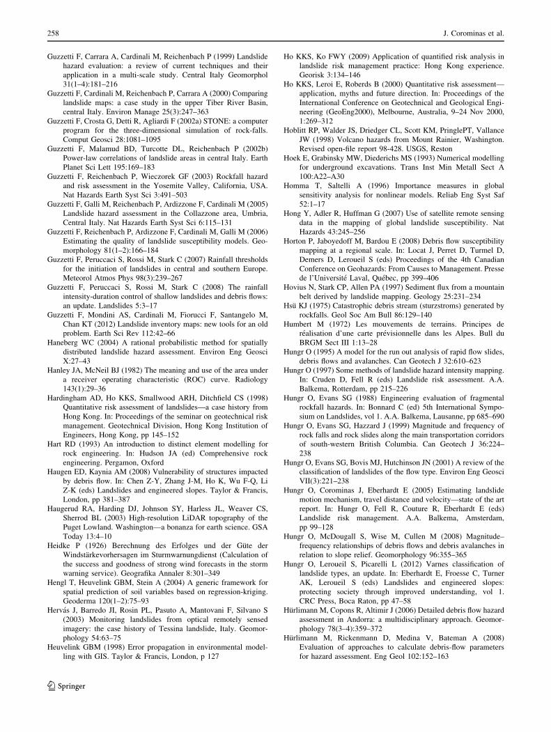
Guzzetti F, Carrara A, Cardinali M, Reichenbach P (1999) Landslide

hazard evaluation: a review of current techniques and their

application in a multi-scale study. Central Italy Geomorphol

31(1–4):181–216

Guzzetti F, Cardinali M, Reichenbach P, Carrara A (2000) Comparing

landslide maps: a case study in the upper Tiber River Basin,

central Italy. Environ Manage 25(3):247–363

Guzzetti F, Crosta G, Detti R, Agliardi F (2002a) STONE: a computer

program for the three-dimensional simulation of rock-falls.

Comput Geosci 28:1081–1095

Guzzetti F, Malamud BD, Turcotte DL, Reichenbach P (2002b)

Power-law correlations of landslide areas in central Italy. Earth

Planet Sci Lett 195:169–183

Guzzetti F, Reichenbach P, Wieczorek GF (2003) Rockfall hazard

and risk assessment in the Yosemite Valley, California, USA.

Nat Hazards Earth Syst Sci 3:491–503

Guzzetti F, Galli M, Reichenbach P, Ardizzone F, Cardinali M (2005)

Landslide hazard assessment in the Collazzone area, Umbria,

Central Italy. Nat Hazards Earth Syst Sci 6:115–131

Guzzetti F, Reichenbach P, Ardizzone F, Cardinali M, Galli M (2006)

Estimating the quality of landslide susceptibility models. Geo-

morphology 81(1–2):166–184

Guzzetti F, Peruccaci S, Rossi M, Stark C (2007) Rainfall thresholds

for the initiation of landslides in central and southern Europe.

Meteorol Atmos Phys 98(3):239–267

Guzzetti F, Peruccaci S, Rossi M, Stark C (2008) The rainfall

intensity-duration control of shallow landslides and debris flows:

an update. Landslides 5:3–17

Guzzetti F, Mondini AS, Cardinali M, Fiorucci F, Santangelo M,

Chan KT (2012) Landslide inventory maps: new tools for an old

problem. Earth Sci Rev 112:42–66

Haneberg WC (2004) A rational probabilistic method for spatially

distributed landslide hazard assessment. Environ Eng Geosci

X:27–43

Hanley JA, McNeil BJ (1982) The meaning and use of the area under

a receiver operating characteristic (ROC) curve. Radiology

143(1):29–36

Hardingham AD, Ho KKS, Smallwood ARH, Ditchfield CS (1998)

Quantitative risk assessment of landslides—a case history from

Hong Kong. In: Proceedings of the seminar on geotechnical risk

management. Geotechnical Division, Hong Kong Institution of

Engineers, Hong Kong, pp 145–152

Hart RD (1993) An introduction to distinct element modelling for

rock engineering. In: Hudson JA (ed) Comprehensive rock

engineering. Pergamon, Oxford

Haugen ED, Kaynia AM (2008) Vulnerability of structures impacted

by debris flow. In: Chen Z-Y, Zhang J-M, Ho K, Wu F-Q, Li

Z-K (eds) Landslides and engineered slopes. Taylor & Francis,

London, pp 381–387

Haugerud RA, Harding DJ, Johnson SY, Harless JL, Weaver CS,

Sherrod BL (2003) High-resolution LiDAR topography of the

Puget Lowland. Washington—a bonanza for earth science. GSA

Today 13:4–10

Heidke P (1926) Berechnung des Erfolges und der Gute der

Windstarkevorhersagen im Sturmwarnungdienst (Calculation of

the success and goodness of strong wind forecasts in the storm

warning service). Geografika Annaler 8:301–349

Hengl T, Heuvelink GBM, Stein A (2004) A generic framework for

spatial prediction of soil variables based on regression-kriging.

Geoderma 120(1–2):75–93

Hervas J, Barredo JI, Rosin PL, Pasuto A, Mantovani F, Silvano S

(2003) Monitoring landslides from optical remotely sensed

imagery: the case history of Tessina landslide, Italy. Geomor-

phology 54:63–75

Heuvelink GBM (1998) Error propagation in environmental model-

ling with GIS. Taylor & Francis, London, p 127

Ho KKS, Ko FWY (2009) Application of quantified risk analysis in

landslide risk management practice: Hong Kong experience.

Georisk 3:134–146

Ho KKS, Leroi E, Roberds B (2000) Quantitative risk assessment—

application, myths and future direction. In: Proceedings of the

International Conference on Geotechnical and Geological Engi-

neering (GeoEng2000), Melbourne, Australia, 9–24 Nov 2000,

1:269–312

Hoblitt RP, Walder JS, Driedger CL, Scott KM, PringlePT, Vallance

JW (1998) Volcano hazards from Mount Rainier, Washington.

Revised open-file report 98-428. USGS, Reston

Hoek E, Grabinsky MW, Diederichs MS (1993) Numerical modelling

for underground excavations. Trans Inst Min Metall Sect A

100:A22–A30

Homma T, Saltelli A (1996) Importance measures in global

sensitivity analysis for nonlinear models. Reliab Eng Syst Saf

52:1–17

Hong Y, Adler R, Huffman G (2007) Use of satellite remote sensing

data in the mapping of global landslide susceptibility. Nat

Hazards 43:245–256

Horton P, Jaboyedoff M, Bardou E (2008) Debris flow susceptibility

mapping at a regional scale. In: Locat J, Perret D, Turmel D,

Demers D, Leroueil S (eds) Proceedings of the 4th Canadian

Conference on Geohazards: From Causes to Management. Presse

de l’Universite Laval, Quebec, pp 399–406

Hovius N, Stark CP, Allen PA (1997) Sediment flux from a mountain

belt derived by landslide mapping. Geology 25:231–234

Hsu KJ (1975) Catastrophic debris stream (sturzstroms) generated by

rockfalls. Geol Soc Am Bull 86:129–140

Humbert M (1972) Les mouvements de terrains. Principes de

realisation d’une carte previsionnelle dans les Alpes. Bull du

BRGM Sect III 1:13–28

Hungr O (1995) A model for the run out analysis of rapid flow slides,

debris flows and avalanches. Can Geotech J 32:610–623

Hungr O (1997) Some methods of landslide hazard intensity mapping.

In: Cruden D, Fell R (eds) Landslide risk assessment. A.A.

Balkema, Rotterdam, pp 215–226

Hungr O, Evans SG (1988) Engineering evaluation of fragmental

rockfall hazards. In: Bonnard C (ed) 5th International Sympo-

sium on Landslides, vol 1. A.A. Balkema, Lausanne, pp 685–690

Hungr O, Evans SG, Hazzard J (1999) Magnitude and frequency of

rock falls and rock slides along the main transportation corridors

of south-western British Columbia. Can Geotech J 36:224–

238

Hungr O, Evans SG, Bovis MJ, Hutchinson JN (2001) A review of the

classification of landslides of the flow type. Environ Eng Geosci

VII(3):221–238

Hungr O, Corominas J, Eberhardt E (2005) Estimating landslide

motion mechanism, travel distance and velocity—state of the art

report. In: Hungr O, Fell R, Couture R, Eberhardt E (eds)

Landslide risk management. A.A. Balkema, Amsterdam,

pp 99–128

Hungr O, McDougall S, Wise M, Cullen M (2008) Magnitude–

frequency relationships of debris flows and debris avalanches in

relation to slope relief. Geomorphology 96:355–365

Hungr O, Leroueil S, Picarelli L (2012) Varnes classification of

landslide types, an update. In: Eberhardt E, Froesse C, Turner

AK, Leroueil S (eds) Landslides and engineered slopes:

protecting society through improved understanding, vol 1.

CRC Press, Boca Raton, pp 47–58

Hurlimann M, Copons R, Altimir J (2006) Detailed debris flow hazard

assessment in Andorra: a multidisciplinary approach. Geomor-

phology 78(3–4):359–372

Hurlimann M, Rickenmann D, Medina V, Bateman A (2008)

Evaluation of approaches to calculate debris-flow parameters

for hazard assessment. Eng Geol 102:152–163


123

Hutchinson JN (1986) A sliding-consolidation model for flow slides.

Can Geotech J 23:115–126

IAEG Commission on Landslides (1990) Suggested nomenclature for

landslides. Bull Int Assoc Eng Geol 41:13–16

IUGS Working Group on Landslides, Committee on Risk Assessment

(1997) Quantitative risk assessment for slopes and landslides—

the state of the art. In: Cruden D, Fell R (eds) Landslide risk

assessment. A.A. Balkema, Amsterdam, pp 3–12

Iverson RM (2000) Landslide triggering by rain infiltration. Water

Resour Res 36:1897–1910

Iverson RI, Denlinger RP (2001) Flow of variably fluidized granular

masses across three dimensional terrain. Coulomb mixture

theory. J Geophys Res 106(B1):537–552

Iverson RM, Schilling SP, Vallance JW (1998) Objective delineation

of lahar-inundation hazard zones. Geol Soc Am Bull

110(8):972–984

Jaboyedoff M (2003) Conefall v.10: a program to estimate propaga-

tion zones of rockfall, based on cone method. Quanterra,

Lausanne. http://www.quanterra.com

Jaboyedoff M, Labiouse V (2003) Preliminary assessment of rockfall

hazard based on GIS data. In: ISRM 2003: Technology Roadmap

for Rock Mechanics, Gauteng, South Africa, 8–12 Sept 2003,

pp 575–578

Jaboyedoff M, Labiouse V (2011) Preliminary estimation of rockfall

runout zones. Nat Hazards Earth Syst Sci 11:819–828

Jaboyedoff M, Dudt JP, Labiouse V (2005) An attempt to refine

rockfall hazard zoning based on the kinetic energy, frequency

and fragmentation degree. Nat Hazards Earth Syst Sci 5:621–632

Jaboyedoff M, Oppikofer T, Abellan A, Derron M-H, Loye A,

Metzger R, Pedrazzini A (2012) Use of LIDAR in landslide

investigations: a review. Nat Hazards 61(1):5–28

Jaiswal P, van Westen CJ (2009) Estimating temporal probability for

landslide initiation along transportation routes based on rainfall

thresholds. Geomorphology 112:96–105

Jaiswal P, van Westen CJ, Jetten V (2010) Quantitative assessment of

direct and indirect landslide risk along transportation lines in

southern India. Nat Hazards Earth Syst Sci 10(6):1253–1267

Jaiswal P, van Westen CJ, Jetten V (2011) Quantitative estimation of

landslide risk from rapid debris slides on natural slopes in

the Nilgiri hills, India. Nat Hazards Earth Syst Sci 11:1723–

1743

Jakob M (1996) Morphometric and geotechnical controls of debris-

flow frequency and magnitude in southwestern British Columbia.

Ph.D. thesis. Geography Department, The University of British

Columbia, Vancouver

Jakob M (2005) A size classification for debris flows. Eng Geol

79:151–161

Jakob M (2012) The fallacy of frequency. Statistical techniques for

debris flow frequency magnitude analysis. In: Proceedings of the

International Landslide Conference, Banff, Canada, 2–8 June

2012, 1:741–750

Jakob M, Friele P (2010) Frequency and magnitude of debris flows on

Cheekye River British Columbia. Geomorphology 114:382–395

Jakob M, Weatherly H (2005) Debris flow hazard and risk assess-

ment. Jones Creek, Washington. In: Hungr O, Fell R, Couture R,

Eberhardt E (eds) Landslide risk management proceedings.

Taylor & Francis, London, pp 533–542

Jakob M, Stein D, Ulmi M (2012) Vulnerability of buildings to debris

flow impact. Nat Hazards 60:241–261

Jibson RW, Harp EL, Michael JA (1998) A method for producing

digital probabilistic seismic landslide hazard maps: an example

from the Los Angeles, California, area. Open file report. US

Geological Survey, Reston, pp 98–113

Jones CL, Higgins JD Andrew RD (2000) Colorado Rock Fall

Simulation Program, version 40. Colorado Department of

Transportation, Colorado Geological Survey, Denver

Jongmans D, Garambois S (2007) Geophysical investigation of

landslides: a review. Bull Soc Geol France 178:101–112

Kaab A (2010) Photogrammetry for early recognition of high

mountain hazards: new techniques and applications. Phys Chem

Earth Part B 25(9):765–770

Kanungo DP, Arora MK, Sarkar S, Gupta RP (2006) A comparative

study of conventional, ANN black box, fuzzy and combined

neural and fuzzy weighting procedures for landslide suscepti-

bility zonation in Darjeeling Himalayas. Eng Geol

85(3–4):347–366

Kappes M, Keiler M, Glade T (2010) From single- to multi-hazard

risk analyses: a concept addressing emerging challenges. In:

Malet JP, Glade T, Casagli N (ed) Proc Int Conf on Mountain

Risks: Bringing Science to Society, Firenze, Italy, 24–26 Nov

2010, pp 351–356

Kaynia AM, Papathoma-Kohle M, Neuhauser B, Ratzinger K,

Wenzel H, Medina-Cetina Z (2008) Probabilistic assessment of

vulnerability to landslide: application to the village of Lichten-

stein, Baden-Wurttemberg, Germany. Eng Geol 101:33–48

Keefer DK (1984) Landslides caused by earthquakes. Geol Soc Am

Bull 95(4):406–421

Keefer DK (2002) Investigating landslides caused by earthquakes—a

historical review. Surv Geophys 23:473–510

Kienholz H (1978) Map of geomorphology and natural hazards of

Grindelwald, Switzerland, scale 1:10,000. Artic Alp Res

10:169–184

King D, MacGregor C (2000) Using social indicators to measure

community vulnerability to natural hazards. Aust J Emerg

Manag 15(3):52–57

Koutsourelakis PS (2010) Assessing structural vulnerability against

earthquakes using multi-dimensional fragility surfaces: a Bayes-

ian framework. Probab Eng Mech 25:49–60

Kramer SL (1996) Geotechnical earthquake engineering. Prentice-

Hall, Englewood Cliffs

Kuriakose SL (2010) Physically-based dynamic modelling of the

effect of land use changes on shallow landslide initiation in the

Western Ghats of Kerala, India. Ph.D. thesis. University of

Utrecht, Utrecht, ISBN 978-90-6164-298-5

Kuriakose SL, Devkota S, Rossiter DG, Jetten VJ (2009) Prediction of

soil depth using environmental variables in an anthropogenic

landscape, a case study in the Western Ghats of Kerala, India.

Catena 79(1):27–38

Lacasse S, Eidsvik U, Nadim F, Hoeg K, Blikra LH (2008) Event tree

analysis of Aknes rock slide hazard. In: 4th Canadian Conf on

Geohazards, Quebec City, Canada, 20–24 May 2008,

pp 551–557

Laigle D, Coussot P (1997) Numerical modelling of mudflows.

J Hydraul Eng ASCE 123(7):617–623

Lee S (2005) Application of logistic regression model and its

validation for landslide susceptibility mapping using GIS and

remote sensing data. Int J Remote Sens 26(7):1477–1491

Lee EM, Jones DKC (2004) Landslide risk assessment. Thomas

Telford, London, p 454

Lee EM, Brunsden D, Sellwood M (2000) Quantitative risk assess-

ment of coastal landslide problems. In: Bromhead E, Dixon N,

Ibsen M-L (eds) Landslides in Research Theory and Practice:

Eighth International Symposium on Landslides. Thomas Telford,

London, 2:899–904

Lee EM, Meadowcroft IC, Hall JW, Walkden M (2002) Coastal

landslide activity: a probabilistic simulation model. Bull Eng

Geol Environ 61:347–355

Lee S, Ryu J-H, Won J-S, Park H-J (2004) Determination and

application of the weights for landslide susceptibility mapping

using an artificial neural network. Eng Geol 71(3–4):289–302

Leroi E, Bonnard Ch, Fell R, McInnes R (2005) Risk assessment and

management—state of the art report. In: Hungr O, Fell R,


123

http://www.quanterra.com

Couture R, Eberhardt E (eds) Landslide risk management. A.A.

Balkema, Amsterdam, pp 159–198

Leroueil S (2001) Natural slopes and cuts: movement and failure

mechanisms. Geotechnique 51(3):197–243

Leroueil S, Locat J, Vaunat J, Picarelli L, Faure R (1996)

Geotechnical characterisation of slope movements. In: Proc

VII Int Symp on Landslides, Trondheim, Norway, 17–21 June

1996, 1:53–74

Lewis J (1984) Multi-hazard history of Antigua. Disasters

8(3):190–197

Li T (1983) A mathematical model for predicting the extent of a

major rockfall. Z Geomorphol 24:473–482

Li Z, Nadim F, Huang H, Uzielli M, Lacasse S (2010) Quantitative

vulnerability estimation for scenario-based landslide hazards.

Landslides 7(2):125–134

Lopez Saez J, Corona C, Stoffel M, Schoeneich P, Berger F (2012)

Probability maps of landslide reactivation derived from tree-ring

records: Pra Bellon landslide, southern French Alps. Geomor-

phology 138:189–202

Lu P, Stumpf A, Kerle N, Casagli N (2011) Object-oriented change

detection for landslide rapid mapping. IEEE Geosci Remote

Sens Lett 99:701–705

Luzi L (1995) Application of favourability modelling to zoning of

landslide hazard in the Fabriano Area, Central Italy. In: Proc

First Joint Eur Conf & Exhibition on Geographical Information,

The Hague, Netherlands, 26–31 March 1995, pp 398–402

Malamud BD, Turcotte DL, Guzzetti F, Reichenbach P (2004)

Landslide inventories and their statistical properties. Earth Surf

Proc Land 29:687–711

Malet J-P, Maquaire O, Locat J, Remaıtre A (2004) Assessing debris

flow hazard associated with slow moving landslides: methodol-

ogy and numerical analyses. Landslides J Int Consortium

Landslides 1:83–90

Malet J-P, van Asch ThWJ, van Beek R, Maquaire O (2005)

Forecasting the behaviour of complex landslides with a spatially

distributed hydrological model. Nat Hazards Earth Syst Sci

5(1):71–85

Mansour MF, Morgenstern NI, Martin CD (2011) Expected damage

from displacement of slow-moving slides. Landslides

8(1):117–131

Martha TR, Kerle N, Jetten V, van Westen CJ, Kumar KV (2010a)

Characterising spectral, spatial and morphometric properties of

landslides for semi-automatic detection using object-oriented

methods. Geomorphology 116(1–2):24–36

Martha TR, Kerle N, Jetten V, van Westen CJ, Vinod Kumar K

(2010b) Landslide volumetric analysis using Cartosat-1-derived

DEMs. Geosci Remote Sens Lett EEE 7(3):582–586

Marzocchi W, Garcia-Aristizabal A, Gasparini P, Mastellone ML, Di

Ruocco A (2012) Basic principles of multi-risk assessment: a

case study in Italy. Nat Hazards 62:551–573

Matthews JA, Brunsden D, Frenzel B, Glaser B, Weiß MM (1997)

Rapid mass movement as a source of climatic evidence for the

Holocene. Paleoclimate Res 19:444

Mavrouli O, Corominas J (2010a) Rockfall vulnerability assessment

for reinforced concrete buildings. Nat Hazards Earth Syst Sci

10:2055–2066

Mavrouli O, Corominas J (2010b) Vulnerability of simple reinforced

concrete buildings in front of the rockfall impact. Landslides

7(2):169–180

McDougall S, Hungr O (2004) A model for the analysis of rapid

landslide run out motion across three dimensional terrain. Can

Geotech J 41:1084–1097

Melchiorre C, Frattini P (2012) Modelling probability of rainfall-

induced shallow landslides in a changing climate, Otta, Central

Norway. Clim Chang 113(2):413–436

Melchiorre C, Castellanos Abella EA, van Westen CJ, Matteucci M

(2011) Evaluation of prediction capability, robustness, and

sensitivity in non-linear landslide susceptibility models, Guanta-

namo, Cuba. Comput Geosci 37(4):410–425

METI/NASA (2009) ASTER Global Digital Elevation Model.

Ministry of Economy, Trade and Industry of Japan (METI)/

National Aeronautics and Space Administration (NASA),

Tokyo/Washington, DC. http://asterweb.jpl.nasa.gov/gdem.asp

and http://www.gdem.ersdac.jspacesystems.or.jp

Metternicht G, Hurni L, Gogu R (2005) Remote sensing of landslides:

an analysis of the potential contribution to geo-spatial systems

for hazard assessment in mountainous environments. Remote

Sens Environ 98(23):284–303

Meunier P, Hovius N, Haines AJ (2007) Regional patterns of

earthquake-triggered landslides and their relation to ground

motion. Geophys Res Lett 34(20):L20408

Michoud C, Abellan A, Derron MH, Jaboyedoff M (eds) (2010)

SafeLand Deliverable D4.1: review of techniques for landslide

detection, fast characterization, rapid mapping and long-term

monitoring. Available at http://www.safeland-fp7.eu/

Michoud C, Derron MH, Hortin P, Jaboyedoff M, Baillifard FJ, Loye

A, Nicolet P, Pedrazzini A, Queyrel A (2012) Rockfall hazard

and risk assessments along roads at a regional scale: example in

Swiss Alps. Nat Hazards Earth Syst Sci 12:615–629

Miles SB, Keefer DK (2009) Evaluation of CAMEL—comprehensive

areal model of earthquake-induced landslides. Eng Geol

104:1–15

Miller DJ, Sias J (1998) Deciphering large landslides: linking

hydrological groundwater and stability models through GIS.

Hydrol Process 12:923–941

Mondini AC, Guzzetti F, Reichenbach P, Rossi M, Cardinali M,

Ardizzone M (2011) Semiautomatic recognition and mapping of

rainfall induced shallow landslides using optical satellite images.

Remote Sens Environ 115(7):1743–1757

Montgomery DR, Dietrich WE (1994) A physically based model for

the topographic control on shallow landsliding. Water Resour

Res 30(4):1153–1171

Nadim F, Kjeksta O (2009) Assessment of global high-risk landslide

disaster hotspots. In: Sassa K, Canuti P (eds) Landslides—diaster

risk reduction. Springer, Berlin, pp 213–221

Nadim F, Kjekstad O, Peduzzi P, Herold C, Jaedicke C (2006) Global

landslide and avalanche hotspots. Landslides 3(2):159–174

Negulescu C, Foerster E (2010) Parametric studies and quantitative

assessment of the vulnerability of a RC frame building exposed

to differential settlements. Nat Hazards Earth Syst Sci 10:

1781–1792

Nelson A, Reute HI, Gessler P (2009) Chapter 3: DEM production

methods and sources. In: Hengl T, Reute HI (eds) Developments

in soil science, vol 33. Elsevier, Amsterdam, pp 65–85

NIBS (2004) Earthquake loss estimation methodology HAZUS.

National Institute of Building Sciences, FEMA, Washington, DC

Nielson BG, DesRoches R (2007) Analytical seismic fragility curves

for typical bridges in the Central and Southeastern United States.

Earthq Spectra 23(3):615

Niethammer U, James MR, Rothmund S, Travelletti J, Joswig M

(2011) Very high spatial resolution monitoring of the Super-

Sauze landslide with an UAV-based remote sensing technique.

Eng Geol. doi:101016/jenggeo201103012

OFAT, OFEE, OFEFP (1997) Recommandations 1997: prise en

compte des dangers dus aux mouvements de terrain dans le cadre

des activites de l’amenagement du territoire. OCFIM, Berne,

p 42

Ohlmacher GC, Davis JC (2003) Using multiple logistic regression

and GIS technology to predict landslide hazard in northeast

Kansas. USA Eng Geol 69(33):331–343


123

http://asterweb.jpl.nasa.gov/gdem.asp

http://www.gdem.ersdac.jspacesystems.or.jp


http://dx.doi.org/101016/jenggeo201103012

Pack RT, Tarboton DG, Goodwin CN (1998) The SINMAP approach

to terrain stability mapping. In: 8th Congr Int Assoc Eng Geol,

Vancouver, Canada, 21–25 Sept 1998

Papathoma-Kohle M, Keiler M, Totschnig R, Glade T (2012)

Improvement of vulnerability curves using data from extreme

events: a debris-flow event in South Tyrol. Nat Hazards

64:2083–2105

Pastor M, Quecedo M, Fernandez Merodo JA, Herreros MI, Gonzalez

E, Mira P (2002) Modelling tailing dams and mine waste dumps

failures. Geotechnique LII(8):579–592

Pastor M, Haddad B, Sorbino G, Cuomo S, Drempetic V (2009) A

depth-integrated, coupled SPH model for flow-like landslides

and related phenomena. Int J Numer Anal Meth Geomech

33:143–172

Peirce CS (1884) The numerical measure of the success of

predictions. Science 4:453–454

Pelletier JD, Malamud BD, Blodgett T, Turcotte DL (1997) Scale-

invariance of soil moisture variability and its implications for the

frequency–size distribution of landslides. Eng Geol 48:255–268

Penızek V, Boruvka L (2006) Soil depth prediction supported by

primary terrain attributes: a comparison of methods. Plant Soil

Environ 52(9):424–430

Petley DN (2012) Landslides and engineered slopes: protecting

society through improved understanding. In: Eberhardt E, Froese

C, Turner AK, Leroueil S (eds) Landslides and engineered

slopes, vol 1. CRC, London, pp 3–13

Pfeiffer TJ, Bowen TD (1989) Computer simulations of rockfalls.

Bull Assoc Eng Geol 26:135–146

Pike RJ (2000) Geomorphometry—diversity in quantitative surface

analysis. Prog Phys Geogr 24(1):1–20

Pinyol NM, Alonso EE (2010) Criteria for rapid sliding II: thermo-

hydro-mechanical and scale effects in Vaiont case. Eng Geol

114:211–227

Piteau DR, Clayton R (1976) Computer rockfall model. In: Proc

Meeting on Rockfall Dynamics and Protective Work Effective-

ness, ISMES, Bergamo, Italy, 20–21 May 1976, pp 123–125

Pitilakis K, Fotopoulou S et al (eds) (2011) SafeLand Deliverable

D2.5: physical vulnerability of elements at risk to landslides:

methodology for evaluation, fragility curves and damage states

for buildings and lifelines. Available at http://www.safeland-fp7.

eu/

Porter K, Eeri M, Kennedy R, Bachman R (2007) Creating fragility

functions for performance-based earthquake engineering. Back-

ground Object Eng 23(2):471–489

Prochaska AB, Santi PM, Higgins JD, Cannon SH (2008) Debris-flow

runout predictions based on the average channel slope (ACS).

Eng Geol 98:29–40

Provost F, Fawcett T (1997) Analysis and visualization of classifier

performance: comparison under imprecise class and cost distri-

butions. In: Proceedings of the Third International Conference

on Knowledge Discovery and Data Mining. AAAI, Menlo Park,

pp 43–48

Provost F, Fawcett T (2001) Robust classification for imprecise

environments. Mach Learn 42(3):203–231

Quan Luna B, Blahut J, Van Westen CJ, Sterlacchini S, van Asch

TWJ, Akbas SO (2011) The application of numerical debris flow

modelling for the generation of physical vulnerability curves.

Nat Hazards Earth Syst Sci 11:2047–2060. doi:10.5194/nhess-

11-2047-2011

Quecedo M, Pastor M, Herreros MI, Fernandez Merodo JA (2004)

Numerical modelling of the propagation of fast landslides using

the finite element method. Int J Numer Meth Eng 59(6):755–794

Quinn PE, Hutchinson DJ, Diederichs MS, Rowe RK (2011)

Characteristics of large landslides in sensitive clay in relation

to susceptibility, hazard, and risk. Can Geotech J 48:1212–

1232

Razak KA, Straatsma MW, van Westen CJ, Malet J-P, de Jong SM

(2011) Airborne laser scanning of forested landslides character-

ization: terrain model quality and visualization. Geomorphology

126:186–200

Reid LM, Page MJ (2003) Magnitude and frequency of landsliding in

a large New Zealand catchment. Geomorphology 49:71–88

Remondo J, Bonachea J, Cendrero A (2005) A statistical approach to

landslide risk modelling at basin scale: from landslide suscep-

tibility to quantitative risk assessment. Landslides 2:321–328

Remondo J, Bonachea J, Cendrero A (2008) Quantitative landslide

risk assessment and mapping on the basis of recent occurrences.


Rickenmann D (1999) Empirical relationships for debris flows. Nat

Hazards 19:47–77

Rickenmann D (2005) Runout prediction methods. In: Jakob M,

Hungr O (eds) Debris-flow hazards and related phenomena.

Praxis, Chichester, pp 305–324

Roberds W (2005) Estimating temporal and spatial variability and

vulnerability. In: Hungr O, Fell R, Couture R, Eberhardt E (eds)

Landslide risk management. Taylor & Francis, London,

pp 129–158

Roberds WJ, Ho KKS (1997) A quantitative risk assessment and risk

management methodology for natural terrain in Hong Kong. In:

First ASCE Int Conf on Debris-Flow Hazards Mitigation:

Mechanics, Prediction and Assessment, San Francisco, CA,

USA, 7–9 Aug 1997

Romeo R, Floris M, Veneri F (2006) Area-scale landslide hazard and

risk assessment. Environ Geol 51:1–13

Rossi M, Guzzetti F, Reichenbach P, Mondini AC, Peruccacci S

(2010) Optimal landslide susceptibility zonation based onmultiple forecasts. Geomorphology 114(3):129–142

Salciarini D, Godt JW, Savage WZ, Baum RL, Conversini P (2008)

Modelling landslide recurrence in Seattle, Washington, USA.

Eng Geol 102(3–4):227–237

Saltelli A, Tarantola A, Campolongo F, Ratto M (2004) Sensitivity

analysis in practice—a guide to assessing scientific models.

Wiley, Chichester

Santacana N, Baeza B, Corominas J, De Paz A, Marturia J (2003) A

GIS-based multivariate statistical analysis for shallow landslide

susceptibility mapping in La Pobla de Lillet area (Eastern

Pyrenees, Spain). Nat Hazards 30:281–295

Savage SB, Hutter K (1991) The dynamics of avalanches of granular

materials from initiation to runout. Part I Anal Acta Mech

86:201–223

Savage WZ, God JW, Baum RL (2004) Modelling time-dependent

areal slope instability. In: Lacerda W, Ehrlich M, Fountoura

SAB, Sayao ASF (eds) Landslide Evaluation and Stabilization:

IX International Symposium on Landslides, Rio de Janeiro, vol

1. A.A. Balkema, Amsterdam, pp 23–38

Saygili G, Rathje EM (2009) Probabilistically based seismic landslide

hazard maps: an application in Southern California. Eng Geol

109:183–194

Scheidegger A (1973) On the prediction of the reach and velocity of

catastrophic landslides. Rock Mech 5:231–236

Scheidl C, Rickenmann D (2010) Empirical prediction of debris-flow

mobility and deposition on fans. Earth Surf Process Landf

35:157–173

Schmidt J, Matcham I, Reese S, King A, Bell R, Henderson R, Smart

G, Cousins J, Smith W, Heron D (2011) Quantitative multi-risk

analysis for natural hazards: a framework for multi-risk model-

ling. Nat Hazard 58:1169–1192. doi:101007/s11069-011-9721-z

Schuster RL, Logan RL, Pringle PT (1992) Prehistoric rock

avalanches in the Olympic Mountains. Wash Sci 258:1620–1621

Shinozuka M, Feng MQ, Lee J, Naganuma T (2000) Statistical

analysis of fragility curves. J Eng Mech ASCE 126(12):

1224–1231


123



http://dx.doi.org/10.5194/nhess-11-2047-2011

http://dx.doi.org/10.5194/nhess-11-2047-2011

http://dx.doi.org/101007/s11069-011-9721-z

Shrestha HK, Yatabe R, Bhandary NP (2008) Groundwater flow

modelling for effective implementation of landslide stability

enhancement measures. Landslides 5:281–290

Simoni S, Zanotti F, Bertoldi G, Rigon R (2008) Modelling the

probability of occurrence of shallow landslides and channelized

debris flows using GEOtop-FS. Hydrol Process 22:532–545

Singhroy V (2005) Remote sensing of landslides. In: Glade T,

Anderson M, Crozier MJ (eds) Landslide hazard and risk. Wiley,

Chichester, pp 469–492

Smith MJ, Pain CF (2009) Applications of remote sensing in

geomorphology: applications of remote sensing in geomorphol-

ogy. Prog Phys Geogr 33:568

Smith K, Petley DN (2008) Environmental hazards: assessing risk and

reducing disaster. Taylor & Francis, London

Soeters R, van Westen CJ (1996) Slope instability recognition,

analysis and zonation. In: Turner AK, Schuster RL (eds)

Landslides investigation and mitigation. TRB Special Report

247. National Academy Press, Washington, DC, pp 129–177

Sosio R, Crosta GB, Hungr O (2008) Complete dynamic modelling

calibration for the Thurwieser rock avalanche (Italian Central

Alps). Eng Geol 100:11–26

Springman S, Seward L, Casini F, Askerinejad A, Malet J-P,

Spickerman A, Travelletti J (eds) (2011) SafeLand Deliverable

D1.3: analysis of the results of laboratory experiments and of

monitoring in test sites for assessment of the slope response to

precipitation and validation of prediction models. Available at


Squarzoni C, Delacourt C, Allemand P (2003) Nine years of spatial

and temporal evolution of the La Vallette landslide observed by

SAR interferometry. Eng Geol 68:53–66

Stark CP, Hovius N (2001) The characterization of the landslide size

distributions. Geophys Res Lett 28:1091–1094

Stead D, Eberhardt E, Coggan J, Benko B (2001) Advanced

numerical techniques in rock slope stability analysis: applica-

tions and limitations. In: LANDSLIDES—Causes, Impacts and

Countermeasures, Davos, Switzerland, 17–21 June 2001,

pp 615–624

Stephenson DB (2000) Use of the ‘‘odds ratio’’ for diagnosing

forecast skill. Weather Forecast 15:221–232

Sterlacchini S, Ballabio C, Blahut J, Masetti M, Sorichetta A (2011)

A spatial agreement of predicted patterns in landslide suscep-

tibility maps. Geomorphology 125(1):51–61

Stevens W (1998) RocFall: a tool for probabilistic analysis, design of

remedial measures and prediction of rockfalls. MaSc thesis,

University of Toronto, Toronto

Stoffel M (2010) Magnitude–frequency relationships of debris-

flows—a case study based on field surveys and tree-ring records.


Stumpf A, Malet J-P Kerle N (2011) SafeLand Deliverable D4.3:

creation and updating of landslide inventory maps, landslide

deformation maps and hazard mapsas inputs for QRA using

remote-sensing technology. Available at http://www.safeland-

fp7.eu/

Suzen ML, Doyuran V (2004) Data driven bivariate landslide

susceptibility assessment using geographical information sys-

tems: a method and application to Asarsuyu catchment. Turk

Eng Geol 71:303–321

Swets JA (1988) Measuring the accuracy of diagnostic systems.

Science 240(4857):1285–1293

Tacher L, Bonnard C, Laloui L, Parriaux A (2005) Modelling the

behaviour of a large landslide with respect to hydrogeological

and geomechanical parameter heterogeneity. Landslides 2:3–14

Talebi A, Troch PA, Uijlenhoet R (2008) A steady-state analytical

slope stability model for complex hillslopes. Hydrol Process

22(4):546–553

Tapsell S, McCarthy S, Faulkner H, Alexander M (2010) Social

vulnerability to natural hazards. CapHaz-Net WP4 Report. Flood

Hazard Research Centre—FHRC, Middlesex University, Lon-

don. Available at: http://caphaz-net.org/outcomes-results/

CapHaz-Net_WP4_Social-Vulnerability2.pdf

TC32—Technical Committee 32 (Engineering Practice of Risk

Assessment and Management) of the International Society of

Soil Mechanics and Geotechnical Engineering (ISSMGE) (2004)

Risk assessment—glossary of terms. http://www.engmath.dal.ca/

tc32/2004Glossary_Draft1.pdf

Thiery Y, Malet J-P, Sterlacchini S, Puissant A, Maquaire O (2007)

Landslide susceptibility assessment by bivariate methods at large

scales: application to a complex mountainous environment.

Geomorphology 92(1–2):38–59. doi:101016/jgeomorph2007

02020

Travelletti J, Malet J-P, Schmittbuhl J, Toussaint R, Delacourt C,

Stumpf A (2010) A multi-temporal image correlation method to

characterize landslide displacements. Ber Geol B-A 82:50–57

Tsai CC, Chen ZS, Duh CT, Horng FW (2001) Prediction of soil

depth using a soil-landscape regression model: a case study on

forest soils in southern Taiwan. Natl Sci Counc Repub China

Part B Life Sci 25(1):34–39

Tsao TC, Hsu WK, Cheng CT, Lo WC, Chen CY, Chang YL, Ju JP

(2010) A preliminary study of debris flow risk estimation and

management in Taiwan. In: Chen S-C (ed) International

Symposium Interpraevent in the Pacific Rim in Taipei, Taiwan,

26–30 April 2010, pp 930–939

Turner AK, Schuster LR (eds) (1996) Landslides, investigation and

mitigation. Transportation Research Board Special Report 247.

National Research Council, National Academy Press, Washing-

ton, DC, p 673

UN-ISDR (2004) Terminology of disaster risk reduction. United

Nations International Strategy for Disaster Reduction, Geneva.

http://www.unisdr.org/eng/library/lib-terminology-eng%20home.

htm

Uzielli M, Lacasse S (2007) Probabilistic estimation of vulnerability

to landslides. In: Proc 13th Panamerican Conf on Soil Mechanics

and Geotechnical Engineering, Margarita, Venezuela, 16–20

July 2007

Uzielli M, Nadim F, Lacasse S, Kaynia AM (2008) A conceptual

framework for quantitative estimation of physical vulnerability

to landslides. Eng Geol 102:251–256

Valadao P, Gaspar JL, Queiroz G, Ferreira T (2002) Landslides

density map of S Miguel Island, Azores archipelago. Nat Hazard


Van Asch ThWJ, Malet J-P, van Beek LPH, Amitrano D (2007)

Techniques, advances, problems and issues in the modelling of

landslide hazard. Bull Soc Geol France 178(2):6–35

Van Beek LH (2002) Assessment of the influence of changes in

landuse and climate on landslide activity in a Mediterranean

environment. Ph.D. thesis, University of Utrecht, Utrecht, p 363

Van Beek LPH, Van Asch TWJ (2004) Regional assessment of the

effects of land-use change and landslide hazard by means of

physically based modelling. Nat Hazards 30(3):289–304

Van Den Eeckhaut M, Hervas J (2012) State of the art of national

landslide databases in Europe and their potential for assessing

landslide susceptibility, hazard and risk. Geomorphology

139–140:545–558

Van Den Eeckhaut M, Poesen J, Govers G, Verstraeten G, Demoulin

A (2007) Characteristics of the size distribution of recent and

historical landslides in a populated hilly region. Earth Planet Sci

Lett 256:588–603

Van Dine DF, Rodman RF, Jordan P, Dupas J (2005) Kuskonook

Creek, an example of a debris flow analysis. Landslides

2(4):257–265. doi:101007/s10346-005-0017


123




http://caphaz-net.org/outcomes-results/CapHaz-Net_WP4_Social-Vulnerability2.pdf

http://caphaz-net.org/outcomes-results/CapHaz-Net_WP4_Social-Vulnerability2.pdf

http://www.engmath.dal.ca/tc32/2004Glossary_Draft1.pdf

http://www.engmath.dal.ca/tc32/2004Glossary_Draft1.pdf



http://www.unisdr.org/eng/library/lib-terminology-eng%20home.htm

http://www.unisdr.org/eng/library/lib-terminology-eng%20home.htm

http://dx.doi.org/101007/s10346-005-0017

Van Steijn H (1996) Debris-flow magnitude frequency relationships

for mountainous regions of Central and Northern Europe.


Van Westen CJ (1993) Application of geographic information

systems to landslide hazard zonation. Ph.D. dissertation. ITC

publ. no. 15. ITC, Enschede, p 245

Van Westen CJ, Montoya L, Boerhoom L, Coto EB (2002) Multi-

hazard risk assessment using GIS in urban areas: a case study for

the city of Turrialba, Costa Rica. In: Proc Regional Workshop on

Best Practices in Disaster Mitigation: Lessons Learned from the

Asian Urban Disaster Mitigation Program and Other Initiatives,

Bali, Indonesia, 24–26 Sept 2002, pp 53–72

Van Westen CJ, Seijmonsbergen AC, Mantovani F (1999) Comparing

landslide hazard maps. Nat Hazards 20(2–3):137–158

Van Westen CJ, Van Asch TWJ, Soeters R (2005) Landslide hazard

and risk zonation; why is it still so difficult? Bull Eng Geol

Environ 65(2):167–184

Van Westen CJ, Castellanos Abella EA, Sekha LK (2008) Spatial

data for landslide susceptibility, hazards and vulnerability

assessment: an overview. Eng Geol 102(3–4):112–131

Varnes DJ (1984) Landslide hazard zonation: a review of principles

and practice. Natural Hazard Series, vol 3. UNESCO, Paris

Wang KL, Lin MI (2010) Development of shallow seismic landslide

potential map based on Newmark’s displacement: the case study

of Chi–Chi earthquake, Taiwan. Environ Earth Sci 60:775–785

Wechsler SP (2007) Uncertainties associated with digital elevation

models for hydrologic applications: a review. Hydrol Earth Syst

Sci 11:1481–1500

Wieczorek GF (1984) Preparing a detailed landslide-inventory map

for hazard evaluation and reduction. Bull Assoc Eng Geol

21(3):337–342

Wilson RA (2004) The rise and fall of a debris flow warning system

for the San Francisco Bay Region, California. In: Glade T,

Anderson M, Crozier MJ (eds) Landslide hazard and risk. Wiley,

New York, pp 493–516

Wilson RA, Moon AT, Hendricks M, Stewart IE (2005) Application

of quantitative risk assessment to the Lawrence Hargrave Drive

Project, New South Wales, Australia. In: Hungr O, Fell R,

Couture R, Eberhardt E (ed) Landslide risk management. Taylor

& Francis, London, ISBN 04-1538-043X

Winter MG, Smith J, Fotopoulou S, Pitilakis K, Mavrouli O,

Corominas J, Argyroudis S (submitted) Physical vulnerability

of elements at risk to landslides: methodology for evaluation,

fragility curves and damage states for buildings and lifelines.

Bull Eng Geol Env

Wong HN (2005) Landslide risk assessment for individual facilities—

state of the art report. In: Hungr O, Fell R, Couture R, Eberhardt

E (eds) Proceedings of the International Conference on Land-

slide Risk Management. Taylor & Francis, London, pp 237–296

Wong HN, Ho KKS (1998) Overview of risk of old man-made slopes

and retaining walls in Hong Kong. In: Proceedings of the

Seminar on Slope Engineering in Hong Kong. A.A. Balkema,

Hong Kong, pp 193–200

Wong HN, Chen YM, Lam KC (1997a) Factual report on the

November 1993 natural terrain landslides in three study areas on

Lantau Island. GEO Report No 61. Geotechnical Engineering

Office, Hong Kong, p 42

Wong HN, Ho KKS, Chan YC (1997b) Assessment of consequence of

landslides. In: Cruden D, Fell R (eds) Landslide risk assessment.

A.A. Balkema, Rotterdam, pp 111–149

WP/WLI (1993) A suggested method for describing the activity of a

landslide. Bull Int Assoc Eng Geol 47:53–57

Wu TH, Abdel-Latif MA (2000) Prediction and mapping of landslide

hazard. Can Geotech J 37:781–795

Wu TH, Tang WH, Einstein HH (1996) Landslide hazard and risk

assessment. In: Turner AT, Schuster RL (eds) Landslides—

investigation and mitigation. Transportation Research Board

Special Report no. 247. National Academy Press, Washington,

DC, pp 106–118

Xie M, Tetsuro E, Zhou G, Mitani Y (2003) Geographic Information

Systems based three-dimensional critical slope stability analysis

and landslide hazard assessment. J Geotech Geoenviron Eng

129(12):1109–1118

Yin KJ, Yan TZ (1988) Statistical prediction model for slope

instability of metamorphosed rocks. In: Proc 5th Int Symp on

Landslides, vol 2, Lausanne, Switzerland, 10–15 July 1988,

2:1269–1272

Zezere JL, Garcia RAC, Oliveira SC, Reis E (2008) Probabilistic

landslide risk analysis considering direct costs in the area north

of Lisbon (Portugal). Geomorphology 94:467–495

Zinck JA, Lopez J, Metternicht GI, Shrestha DP, Vazquez-Selem L

(2001) Mapping and modelling mass movements and gullies in

mountainous areas using remote sensing and GIS techniques. Int

J Appl Earth Obs Geoinf 3(1):43–53

Zuccaro G, Santo F, De Gregorio D, Di Crescenzo G (2011)

Methodology for buildings at site specific to local scales. In:

Safeland Deliverable D2.5: physical vulnerability of elements at

risk to landslides: methodology for evaluation, fragility curves

and damage states for buildings and lifelines. Available at http://

www.safeland-fp7.eu/


123



recommendations for the quantitative analysis of landslide ... · recommendations for the...

Documents