rapidminer user manual
DESCRIPTION
Updated User Manaul of Rapidminer v.6.0TRANSCRIPT

RapidMiner Studio Manual

©2014 by RapidMiner. All rights reserved.
No part of this publication may be reproduced, stored in a retrieval system, or transmitted, in any form or by means electronic, mechanical, photocopying, or otherwise, without prior written permission of RapidMiner.
Contents
1 Fundamental Terms 1
1.1 Coincidence or not? . . . . . . . . . . . . . . . . . . . . . . . . . . 1
1.2 Fundamental Terms . . . . . . . . . . . . . . . . . . . . . . . . . . 5
1.2.1 Attributes and Target Attributes . . . . . . . . . . . . . . . 6
1.2.2 Concepts and Examples . . . . . . . . . . . . . . . . . . . . 9
1.2.3 Attribute Roles . . . . . . . . . . . . . . . . . . . . . . . . . 10
1.2.4 Value Types . . . . . . . . . . . . . . . . . . . . . . . . . . . 11
1.2.5 Data and Meta Data . . . . . . . . . . . . . . . . . . . . . . 14
1.2.6 Modelling . . . . . . . . . . . . . . . . . . . . . . . . . . . . 15
2 First steps 19
2.1 Installation and First Repository . . . . . . . . . . . . . . . . . . . 20
2.2 Perspectives and Views . . . . . . . . . . . . . . . . . . . . . . . . 21
2.3 Design Perspective . . . . . . . . . . . . . . . . . . . . . . . . . . . 27
2.3.1 Operators and Repositories View . . . . . . . . . . . . . . . 28
2.3.2 Process View . . . . . . . . . . . . . . . . . . . . . . . . . . 31
2.3.3 Operators and Processes . . . . . . . . . . . . . . . . . . . . 31
2.3.4 Further Options of the Process View . . . . . . . . . . . . . 42
2.3.5 Parameters View . . . . . . . . . . . . . . . . . . . . . . . . 45
2.3.6 Help and Comment View . . . . . . . . . . . . . . . . . . . 47
2.3.7 Overview View . . . . . . . . . . . . . . . . . . . . . . . . . 49
2.3.8 Problems and Log View . . . . . . . . . . . . . . . . . . . . 50
3 Design of Analysis Processes 53
3.1 Creating a New Process . . . . . . . . . . . . . . . . . . . . . . . . 53
V
Contents
3.2 Repository Actions . . . . . . . . . . . . . . . . . . . . . . . . . . . 54
3.3 The First Analysis Process . . . . . . . . . . . . . . . . . . . . . . 56
3.3.1 Transforming Meta Data . . . . . . . . . . . . . . . . . . . 58
3.4 Executing Processes . . . . . . . . . . . . . . . . . . . . . . . . . . 68
3.4.1 Looking at Results . . . . . . . . . . . . . . . . . . . . . . . 69
3.4.2 Breakpoints . . . . . . . . . . . . . . . . . . . . . . . . . . . 70
4 Data and Result Visualization 75
4.1 Result Visualization . . . . . . . . . . . . . . . . . . . . . . . . . . 75
4.1.1 Sources for Displaying Results . . . . . . . . . . . . . . . . 76
4.2 About Data Copies and Views . . . . . . . . . . . . . . . . . . . . 79
4.3 Display Formats . . . . . . . . . . . . . . . . . . . . . . . . . . . . 80
4.3.1 Description . . . . . . . . . . . . . . . . . . . . . . . . . . . 81
4.3.2 Tables . . . . . . . . . . . . . . . . . . . . . . . . . . . . . . 81
4.3.3 Charts . . . . . . . . . . . . . . . . . . . . . . . . . . . . . . 86
4.3.4 Graphs . . . . . . . . . . . . . . . . . . . . . . . . . . . . . 89
4.3.5 Special Views . . . . . . . . . . . . . . . . . . . . . . . . . . 92
4.4 Result Overview . . . . . . . . . . . . . . . . . . . . . . . . . . . . 92
5 Repository 95
5.1 The RapidMiner Studio Repository . . . . . . . . . . . . . . . . . . 95
5.1.1 Creating a New Repository . . . . . . . . . . . . . . . . . . 97
5.2 Using the Repository . . . . . . . . . . . . . . . . . . . . . . . . . . 99
5.2.1 Processes and Relative Repository Descriptions . . . . . . . 99
5.2.2 Importing Data and Objects into the Repository . . . . . . 100
5.2.3 Access to and Administration of the Repository . . . . . . . 103
5.2.4 The Process Context . . . . . . . . . . . . . . . . . . . . . . 104
5.3 Data and Meta Data . . . . . . . . . . . . . . . . . . . . . . . . . . 106
5.3.1 Propagating Meta Data from the Repository and through
the Process . . . . . . . . . . . . . . . . . . . . . . . . . . . 108
VI
1 Motivation andFundamental Terms
In this chapter we would like to give you a small incentive for using data mining
and at the same time also give you an introduction to the most important terms.
Whether you are already an experienced data mining expert or not, this chapter
is worth reading in order for you to know and have a command of the terms used
both here and in RapidMiner.
1.1 Coincidence or not?
Before we get properly started, let us try a small experiment:
• Think of a number between 1 and 10.
• Multiply this number by 9.
• Work out the checksum of the result, i.e. the sum of the numbers.
• Multiply the result by 4.
• Divide the result by 3.
• Deduct 10.
The result is 2.
1
1. Fundamental Terms
Do you believe in coincidence? As an analyst you will probably learn to answer
this question in the negative or even do so already. Let us take for example what
is probably the simplest random event you could imagine, i.e. the toss of a coin.
“Ah” you may think, “but that is a random event and nobody can predict which
side of the coin will be showing after it is tossed”. That may be correct, but
the fact that nobody can predict it does in no way mean that it is impossible in
principle. If all influence factors such as the throwing speed and rotation angle,
material properties of the coin and those of the ground, mass distributions and
even the strength and direction of the wind were all known exactly, then we would
be quite able, with some time and effort, to predict the result of such a coin toss.
The physical formulas for this are all known in any case.
We shall now look at another scenario, only this time we can predict the outcome
of the situation: A glass will break if it falls from a certain height onto a certain
type of ground. We even know in the fractions of the second when the glass
is falling: There will be broken glass. How are we able to achieve this rather
amazing feat? We have never seen the glass which is falling in this instant break
before and the physical formulas that describe the breakage of glass are a complete
mystery for most of us at least. Of course, the glass may stay intact “by chance”
in individual cases, but this is not likely. For what it’s worth, the glass not
breaking would be just as non-coincidental, since this result also follows physical
laws. For example, the energy of the impact is transferred to the ground better
in this case. So how do we humans know what exactly will happen next in some
cases and in other cases, for example that of the toss of a coin, what will not?
The most frequent explanation used by laymen in this case is the description of
the one scenario as “coincidental” and the other as “non-coincidental”. We shall
not go into the interesting yet nonetheless rather philosophical discussions on this
topic, but we are putting forward the following thesis:
The vast majority of processes in our perceptible environment are not a result
of coincidences. The reason for our inability to describe and extrapolate the
processes precisely is rather down to the fact that we are not able to recognise or
measure the necessary influence factors or correlate these.
2
1.1. Coincidence or not?
In the case of the falling glass, we quickly recognised the most important char-
acteristics such as the material, falling height and nature of the ground and can
already estimate, in the shortest time, the probability of the glass breaking by
analogy reasoning from similar experiences. However, it is just that we cannot
do with the toss of a coin. We can watch as many tosses of a coin as we like; we
will never manage to recognise the necessary factors fast enough and extrapolate
them accordingly in the case of a random throw.
So what were we doing in our heads when we made the prediction for the state
of the glass after the impact? We measured the characteristics of this event. You
could also say that we collected data describing the fall of the glass. We then
reasoned very quickly by analogy, i.e. we made a comparison with earlier falling
glasses, cups, porcelain figurines or similar articles based on a similarity measure.
Two things are necessary for this: firstly, we need to also have the data of earlier
events available and secondly, we need to be aware of how a similarity between
the current and past data is defined at all. Ultimately we are able to make an
estimation or prediction by having looked at the most similar events that have
already taken place for example. Did the falling article break in these cases or
not? We must first find the events with the greatest similarity, which represents
a kind of optimisation. We use the term”optimisation“ here, since it is actually
unimportant whether we are now maximising a similarity or the sales figures of
one enterprise or any other - the variable concerned, so similarity here, is always
optimised. The analogy reasoning described then tells us that the majority of
glasses we have already looked at broke and this very estimation then becomes
our prediction. This may sound complicated, but this kind of analogy reasoning
is basically the foundation for almost every human learning process and is done
at a staggering speed.
The interesting thing about this is that we have just been acting as a human data
mining method, since data analysis usually involves matters such as the repre-
sentation of events or conditions and the data resulting from this, the definition
of events’ similarities and of the optimisation of these similarities.
However, the described procedure of analogy reasoning is not possible with the
toss of a coin: It is usually insufficient at the first step and the data for factors
3
1. Fundamental Terms
such as material properties or ground unevenness cannot be recorded. Therefore
we cannot have these ready for later analogy reasoning. This does in no way mean
however that the event of a coin toss is coincidental, but merely shows that we
humans are not able to measure these influence factors and describe the process.
In other cases we may be quite able to measure the influence factors, but we are
not able to correlate these purposefully, meaning that computing similarity or
even describing the processes is impossible for us.
It is by no means the case that analogy reasoning is the only way of deducing
forecasts for new situations from already known information. If the observer of
a falling glass is asked how he knows that the glass will break, then the answer
will often include things like “every time I have seen a glass fall from a height of
more than 1.5 metres it has broken”. There are two interesting points here: The
relation to past experiences using the term “always” as well as the deduction of
a rule from these experiences:
If the falling article is made of glass and the falling height is more than 1.5 metres,
then the glass will break.
The introduction of a threshold value like 1.5 metres is a fascinating aspect of this
rule formation. For although not every glass will break immediately if greater
heights are used and will not necessarily remain intact in the case of lower heights,
introducing this threshold value transforms the rule into a rule of thumb, which
may not always, but will mostly lead to a correct estimate of the situation.
Instead of therefore reasoning by analogy straight away, one could now use this
rule of thumb and would soon reach a decision as to the most probable future
of the falling article. Analogy reasoning and the creation of rules are two first
examples of how humans, and also data mining methods, are able to anticipate
the outcome of new and unknown situations.
Our description of what goes on in our heads and also in most data mining
methods on the computer reveals yet another interesting insight: The analogy
reasoning described does at no time require the knowledge of any physical formula
to say why the glass will now break. The same applies for the rule of thumb
described above. So even without knowing the complete (physical) description
of a process, we and the data mining method are equally able to generate an
4
1.2. Fundamental Terms
estimation of situations or even predictions. Not only was the causal relationship
itself not described here, but even the data acquisition was merely superficial
and rough and only a few factors such as the material of the falling article (glass)
and the falling height (approx. 2m) were indicated, and relatively inaccurately
at that.
Causal chains therefore exist whether we know them or not. In the latter case
we are often inclined to refer to them as coincidental. And it is equally amazing
that describing the further course is possible even for an unknown causal chain,
and even in situations where the past facts are incomplete and only described
inaccurately.
This section has given you an idea of the kind of problems we wish to address
in this book. We will be dealing with numerous influence factors, some of which
can only be measured insufficiently or not at all. At the same time there are
often so many of these factors that we risk losing track. In addition, we also
have to deal with the events which have already taken place, which we wish to
use for modelling and the number of which easily goes into millions or billions.
Last but not least, we must ask ourselves whether describing the process is the
goal or whether analogy reasoning is already sufficient to make a prediction. And
in addition, this must all take place in a dynamic environment under constantly
changing conditions - and preferably as soon as possible. Impossible for humans?
Correct. But not impossible for data mining methods.
1.2 Fundamental Terms
We are now going to introduce some fundamental terms which will make dealing
with the problems described easier for us. You will come across these terms
again and again in the RapidMiner software too, meaning it is worth becoming
acquainted with the terms used even if you are an experienced data analyst.
First of all we can see what the two examples looked at in the previous section,
namely the toss of a coin and the falling glass, have in common. In our discussion
on whether we are able to predict the end of the respective situation, we realised
5
1. Fundamental Terms
that knowing the influence factors as accurately as possible, such as material
properties or the nature of the ground, is important. And one can even try to
find an answer to the question as to whether this book will help you by recording
the characteristics of yourself, the reader, and aligning them with the results
of a survey of some of the past readers. These measured reader characteristics
could be for example the educational background of the person concerned, the
liking of statistics, preferences with other, possibly similar books and further
features which we could also measure as part of our survey. If we now knew such
characteristics of 100 readers and had the indication as to whether you like the
book or not in addition, then the further process would be almost trivial. We
would also ask you the questions from our survey and measure the same features
in this way and then, for example using analogy reasoning as described above,
generate a reliable prediction of your personal taste. “Customers who bought
this book also bought. . . ”. This probably rings a bell.
1.2.1 Attributes and Target Attributes
Whether coins or other falling articles or even humans, there is, as previously
mentioned, the question in all scenarios as to the characteristics or features of the
respective situation. We will always speak of attributes in the following when
we mean such describing factors of a scenario. This is also the term that is always
used in the RapidMiner software when such describing features arise. There are
many synonyms for this term and depending on your own background you will
have already come across different terms instead of “attribute”, for example
• Characteristic,
• Feature,
• Influence factor (or just factor),
• Indicator,
• Variable or
• Signal.
6
1.2. Fundamental Terms
We have seen that description by attributes is possible for processes and also
for situations. This is necessary for the description of technical processes for
example and the thought of the falling glass is not too far off here. If it is
possible to predict the outcome of such a situation then why not also the quality
of a produced component? Or the imminent failure of a machine? Other processes
or situations which have no technical reference can also be described in the same
way. How can I predict the success of a sales or marketing promotion? Which
article will a customer buy next? How many more accidents will an insurance
company probably have to cover for a particular customer or customer group?
We shall use such a customer scenario in order to introduce the remaining im-
portant terms. Firstly, because humans are famously better at understanding
examples about other humans. And secondly, because each enterprise proba-
bly has information, i.e. attributes, regarding their customers and most readers
can therefore relate to the examples immediately. The attributes available as a
minimum, which just about every enterprise keeps about its customers, are for
example geographical data and information as to which products or services the
customer has already purchased. You would be surprised what forecasts can be
made even from such a small amount of attributes.
Let us look at an (admittedly somewhat contrived) example. Let us assume that
you work in an enterprise that would like to offer its customers products in future
which are better tailored to their needs. Within a customer study of only 100
of your customers some needs became clear, which 62 of these 100 customers
share all the same. Your research and development department got straight to
work and developed a new product within the shortest time, which would satisfy
these new needs better. Most of the 62 customers with the relevant needs profile
are impressed by the prototype in any case, although most of the remaining
participants of the study only show a small interest as expected. Still, a total of
54 of the 100 customers in the study said that they found the new product useful.
The prototype is therefore evaluated as successful and goes into production - now
only the question remains as to how, from your existing customers or even from
other potential customers, you are going to pick out exactly the customers with
whom the subsequent marketing and sales efforts promise the greatest success.
You would therefore like to optimise your efficiency in this area, which means in
7
1. Fundamental Terms
particular ruling out such efforts from the beginning which are unlikely to lead
to a purchase. But how can that be done? The need for alternative solutions
and thus the interest in the new product arose within the customer study on a
subset of your customers. Performing this study for all your customers is much
too costly and so this option is closed to you. And this is exactly where data
mining can help. Let us first look at a possible selection of attributes regarding
your customers:
• Name
• Address
• Sector
• Subsector
• Number of employees
• Number of purchases in product group 1
• Number of purchases in product group 2
The number of purchases in the different product groups means the transactions
in your product groups which you have already made with this customer in the
past. There can of course be more or less or even entirely different attributes in
your case, but this is irrelevant at this stage. Let us assume that you have the
information available regarding these attributes for every one of your customers.
Then there is another attribute which we can look at for our concrete scenario:
The fact whether the customer likes the prototype or not. This attribute is of
course only available for the 100 customers from the study; the information on
this attribute is simply unknown for the others. Nevertheless, we also include the
attribute in the list of our attributes:
• Prototype positively received?
• Name
• Address
8
1.2. Fundamental Terms
• Sector
• Subsector
• Number of employees
• Number of purchases in product group 1
• Number of purchases in product group 2
If we assume you have thousands of customers in total, then you can only indicate
whether 100 of these evaluated the prototype positively or not. You do not yet
know what the others think, but you would like to! The attribute “prototype
positively received” thus adopts a special role, since it identifies every one of your
customers in relation to the current question. We therefore also call this special
attribute label, since it sticks to your customers and identifies them like a brand
label on a shirt or even a note on a pinboard. You will also find attributes which
adopt this special role in RapidMiner under the name “label”. The goal of our
efforts is to fill out this particular attribute for the total quantity of all customers.
We will therefore also often speak of target attribute in this book instead of
the term “label”. You will also frequently discover the term goal variable in the
literature, which means the same thing.
1.2.2 Concepts and Examples
The structuring of your customers’ characteristics by attributes, introduced above,
already helps us to tackle the problem a bit more analytically. In this way we
ensured that every one of your customers is represented in the same way. In a
certain sense we defined the type or concept “customer”, which differs consider-
ably from other concepts such as “falling articles” in that customers will typically
have no material properties and falling articles will only rarely buy in product
group 1. It is important that, for each of the problems in this book (or even those
in your own practice), you first define which concepts you are actually dealing
with and which attributes these are defined by.
We implicitly defined above, by indicating the attributes name, address, sector
9
1. Fundamental Terms
etc. and in particular the purchase transactions in the individual product groups,
that objects of the concept “customer” are described by these attributes. Yet this
concept has remained relatively abstract so far and no life has been injected into
it yet. Although we now know in what way we can describe customers, we have
not yet performed this for specific customers. Let us look at the attributes of the
following customer for example:
• Prototype positively received: yes
• Name: Doe Systems, Inc.
• Address: 76 Any Street, Sunnyville, Massachusetts
• Sector: Mechanics
• Subsector: Pipe bending machines
• Number of employees: > 1000
• Number of purchases in product group 1: 5
• Number of purchases in product group 2: 0
We say that this specific customer is an example for our concept “customer”.
Each example can be characterised by its attributes and has concrete values
for these attributes which can be compared with those of other examples. In
the case described above, Doe Systems, Inc. is also an example of a customer
who participated in our study. There is therefore a value available for our target
attribute “prototype positively received?”. Doe Systems was happy and has “yes”
as an attribute value here, thus we also speak of a positive example. Logically,
there are also negative examples and examples which do not allow us to make
any statement about the target attribute.
1.2.3 Attribute Roles
We have now already become acquainted with two different kinds of attributes, i.e.
those which simply describe the examples and those which identify the examples
10
1.2. Fundamental Terms
separately. Attributes can thus adopt different roles. We have already introduced
the role “label” for attributes which identify the examples in any way and which
must be predicted for new examples that are not yet characterised in such a
manner. In our scenario described above the label still describes (if present) the
characteristic of whether the prototype was received positively.
Likewise, there are for example roles, the associated attribute of which serves for
clearly identifying the example concerned. In this case the attribute adopts the
role of an identifier and is called ID for short. You will find such attributes iden-
tified with this role in the RapidMiner software also. In our customer scenario,
the attribute “name” could adopt the role of such an identifier.
There are even more roles, such as those with an attribute that designates the
weight of the example with regard to the label. In this case the role has the name
Weight. Attributes without a special role, i.e. those which simply describe the
examples, are also called regular attributes and just leave out the role desig-
nation in most cases. Apart from that you have the option in RapidMiner of
allocating your own roles and of therefore identifying your attributes separately
in their meaning.
1.2.4 Value Types
As well as the different roles of an attribute there is also a second characteristic of
attributes which is worth looking at more closely. The example of Doe Systems
above defined the respective values for the different attributes, for example “Doe
Systems, Inc.” for the attribute “Name” and the value “5” for the number
of past purchases in product group 1. Regarding the attribute “Name”, the
concrete value for this example is therefore random free text to a certain extent;
for the attribute “number of purchases in product group 1” on the other hand,
the indication of a number must correspond. We call the indication whether
the values of an attribute must be in text or numbers the Value Type of an
attribute.
In later chapters we will become acquainted with many different value types and
see how these can also be transformed into other types. For the moment we just
11

1. Fundamental Terms
need to know that there are different value types for attributes and that we speak
of value type text in the case of free text, of the value type numerical in the case
of numbers and of the value type nominal in the case of only few values being
possible (like with the two possibilities “yes” and “no” for the target attribute).
Please note that in the above example the number of employees, although really
of numerical type, would rather be defined as nominal, since a size class, i.e. “>
1000” was used instead of an exact indication like 1250 employees.
12
1.2. Fundamental Terms
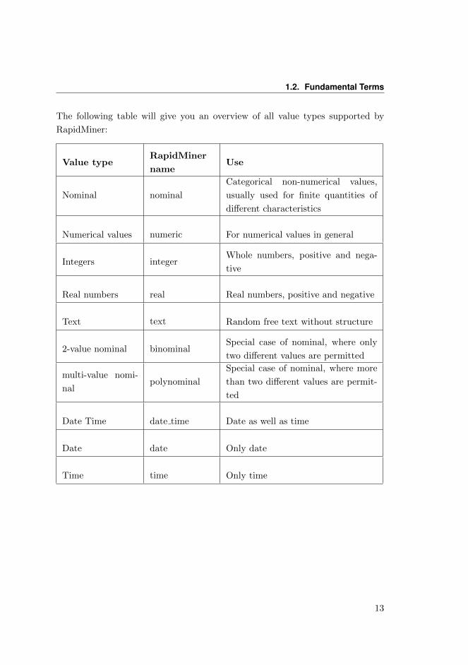
The following table will give you an overview of all value types supported by
RapidMiner:
Value typeRapidMiner
nameUse
Nominal nominal
Categorical non-numerical values,
usually used for finite quantities of
different characteristics
Numerical values numeric For numerical values in general
Integers integerWhole numbers, positive and nega-
tive
Real numbers real Real numbers, positive and negative
Text text Random free text without structure
2-value nominal binominalSpecial case of nominal, where only
two different values are permitted
multi-value nomi-
nalpolynominal
Special case of nominal, where more
than two different values are permit-
ted
Date Time date time Date as well as time
Date date Only date
Time time Only time
13
1. Fundamental Terms
1.2.5 Data and Meta Data
We want to summarise our initial situation one more time. We have a Concept
“customer” available, which we will describe with a set of Attributes:
• Prototype positively received? Label; Nominal
• Name: Text
• Address: Text
• Sector: Nominal
• Subsector: Nominal
• Number of employees: Nominal
• Number of purchases in product group 1: Numerical
• Number of purchases in product group 2: Numerical
The attribute “Prototype positively received?” has a special Role among the
attributes; it is our Target Attribute here. The target attribute has the Value
Type Nominal, which means that only relatively few characteristics (in this
case “yes” and “no”) can be accepted. Strictly speaking it is even binominal,
since only two different characteristics are permitted. The remaining attributes
all have no special role, i.e. they are regular and have either the value type
Numerical or Text. The following definition is very important, since it plays a
crucial role in a successful professional data analysis:
This volume of information which describes a concept is also called meta data,
since it represents data via the actual data.
Our fictitious enterprise has a number of Examples for our concept “customer”,
i.e. the information which the enterprise has stored for the individual attributes in
its customer database. The goal is now to generate a prediction instruction from
the examples for which information is available concerning the target attribute,
which predicts for us whether the remaining customers would be more likely to
14
1.2. Fundamental Terms
receive the prototype positively or reject it. The search for such a prediction
instruction is one of the tasks which can be performed with data mining.
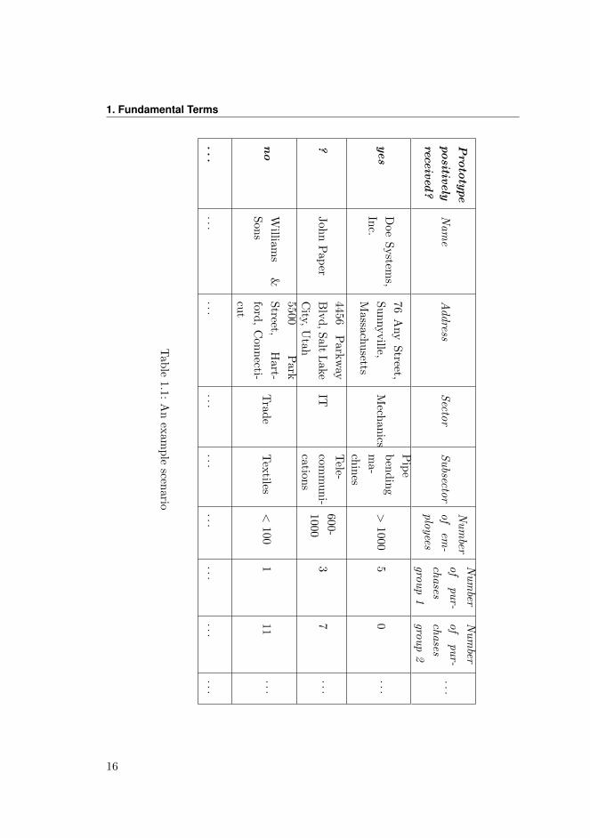
However, it is important here that the information for the attributes of the indi-
vidual examples is in an ordered form, so that the data mining method can access
it by means of a computer. What would be more obvious here than a table? Each
of the attributes defines a column and each example with the different attribute
values corresponds to a row of this table. For our scenario this could look like in
table 1.1 for example.
We call such a table an Example Set, since this table contains the data for all
the attributes of our examples. In the following and also within RapidMiner we
will use the terms Data, Data Set and Example Set synonymously. A table
with the appropriate entries for the attribute values of the current examples is
always meant in this case. It is also such data tables which have lent their name
to data analysis or data mining. Note:
Data describes the objects of a concept, Meta Data describes the characteristics
of a concept (and therefore also of the data).
Most data mining methods expect the examples to be given in such an attribute
value table. Fortunately, this is the case here and we can spare ourselves any
further data transformations. In practice however this is completely different
and the majority of work during a data analysis is time spent transferring the
data into a format suitable for data mining. These transformations are therefore
dealt with in detail in later chapters.
1.2.6 Modelling
Once we have the data regarding our customers available in a well-structured
format, we can then finally replace the unknown values of our target attribute
with the prediction of the most probable value by means of a data mining method.
We have numerous methods available here, many of which, just like the analogy
reasoning described at the beginning or the generating of rules of thumb, are
based on human behaviour. We call the use of a data mining method model and
15
1. Fundamental Terms
Pro
totype
positiv
ely
received
?
Nam
eA
ddress
Secto
rS
ubsecto
r
Nu
mber
of
em-
plo
yees
Nu
mber
of
pu
r-
chases
grou
p1
Nu
mber
of
pu
r-
chases
grou
p2
...
yes
Doe
System
s,
Inc.
76A
ny
Street,
Su
nnyville,
Massach
usetts
Mech
anics
Pip
e
ben
din
g
ma-
chin
es
>1000
50
...
?Joh
nP
aper
4456P
arkw
ay
Blv
d,S
altL
ake
City,
Utah
IT
Tele-
com
mu
ni-
catio
ns
600-
1000
37
...
no
William
s&
Son
s
5500P
ark
Street,
Hart-
ford,
Con
necti-
cut
Trad
eT
extiles
<100
111
...
...
......
......
......
......
Tab
le1.1:
An
exam
ple
scenario
16
1.2. Fundamental Terms
the result of such a method, i.e. the prediction instruction, is a model. Just as
data mining can be used for different issues, this also applies for models. They can
be easy to understand and explain the underlying processes in a simple manner.
Or they can be good to use for prediction in the case of unknown situations.
Sometimes both apply, such as with the following model for example, which a
data mining method could have supplied for our scenario:
“If the customer comes from urban areas, has more than 500 employees and if at
least 3 purchases were transacted in product group 1, then the probability of this
customer being interested in the new product is high.”
Such a model can be easily understood and may provide a deeper insight into
the underlying data and decision processes of your customers. And in addition
it is an operational model, i.e. a model which can be used directly for making
a prediction for further customers. The company “John Paper” for example
satisfies the conditions of the rule above and is therefore bound to be interested
in the new product - at least there is a high probability of this. Your goal would
therefore have been reached and by using data mining you would have generated
a model which you could use for increasing your marketing efficiency: Instead of
just contacting all existing customers and other candidates without looking, you
could now concentrate your marketing efforts on promising customers and would
therefore have a substantially higher success rate with less time and effort. Or
you could even go a step further and analyse which sales channels would probably
produce the best results and for which customers.
In the following chapters we will focus on further uses of data mining and at the
same time practise transferring concepts such as customers, business processes
or products into attributes, examples and data sets. This will train the eye to
detect further possibilities of application tremendously and will make analyst life
much easier for you later on. First though, we would like to spend a little time on
RapidMiner and give a small introduction to its use, so that you can implement
the following examples immediately.
17


2 First steps
RapidMiner Studio combines technology and applicability to serve a user-friendly
integration of the latest as well as established data mining techniques. Defining
analysis processes with RapidMiner Studio is done by drag and drop of operators,
setting parameters and combining operators.
As we will see in the following, processes can be produced from a large number
of almost randomly nestable operators and finally be represented by a so-called
process graph (flow design). The process structure is described internally by
XML and developed by means of a graphical user interface. In the background,
RapidMiner Studio constantly checks the process currently being developed for
syntax conformity and automatically makes suggestions in case of problems. This
is made possible by the so-called meta data transformation, which transforms the
underlying meta data at the design stage in such a way that the form of the re-
sult can already be foreseen and solutions can be identified in case of unsuitable
operator combinations (quick fixes). In addition, RapidMiner Studio offers the
possibility of defining breakpoints and of therefore inspecting virtually every in-
termediate result. Successful operator combinations can be pooled into building
blocks and are therefore available again in later processes.
RapidMiner Studio contains more than 1500 operations altogether for all tasks
of professional data analysis, from data partitioning, to market-based analysis,
to attribute generation, it includes all the tools you need to make your data work
for you. But also methods of text mining, web mining, the automatic sentiment
analysis from Internet discussion forums (sentiment analysis, opinion mining)
as well as the time series analysis and -prediction are available. RapidMiner
19
2. First steps
Studio enables us to use strong visualisations like 3-D graphs, scatter matrices
and self-organizing maps. It allows you to turn your data into fully customizable,
exportable charts with support for zooming, panning, and rescaling for maximum
visual impact.
2.1 Installation and First Repository
Before we can work with RapidMiner Studio, you of course need to download and
install the software first. You will find it in the download area of the RapidMiner
website:
http://www.rapidminer.com
Download the appropriate installation package for your operating system and
install RapidMiner Studio according to the instructions on the website. All usual
Windows versions are supported as well as Macintosh, Linux or Unix systems.
Please note that an up-to-date Java Runtime (at least version 7) is needed for
the latter.
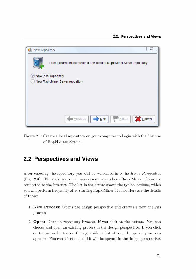
If you are starting RapidMiner Studio for the first time, you will be asked to
create a new repository (Fig. 2.1). We will limit ourselves to a local repository
on your computer first of all - later on you can then define repositories in the
network, which you can also share with others:
For a local repository you just need to specify a name (alias) and define any
directory on your hard drive (Fig. 2.2). You can select the directory directly by
clicking on the folder icon on the right. It is advisable to create a new directory
in a convenient place within the file dialog that then appears and then use this
new directory as a basis for your local repository. This repository serves as a
central storage location for your data and analysis processes and will accompany
you in the near future.
20
2.2. Perspectives and Views
Figure 2.1: Create a local repository on your computer to begin with the first use
of RapidMiner Studio.
2.2 Perspectives and Views
After choosing the repository you will be welcomed into the Home Perspective
(Fig. 2.3). The right section shows current news about RapidMiner, if you are
connected to the Internet. The list in the centre shows the typical actions, which
you will perform frequently after starting RapidMiner Studio. Here are the details
of those:
1. New Process: Opens the design perspective and creates a new analysis
process.
2. Open: Opens a repository browser, if you click on the button. You can
choose and open an existing process in the design perspective. If you click
on the arrow button on the right side, a list of recently opened processes
appears. You can select one and it will be opened in the design perspective.
21
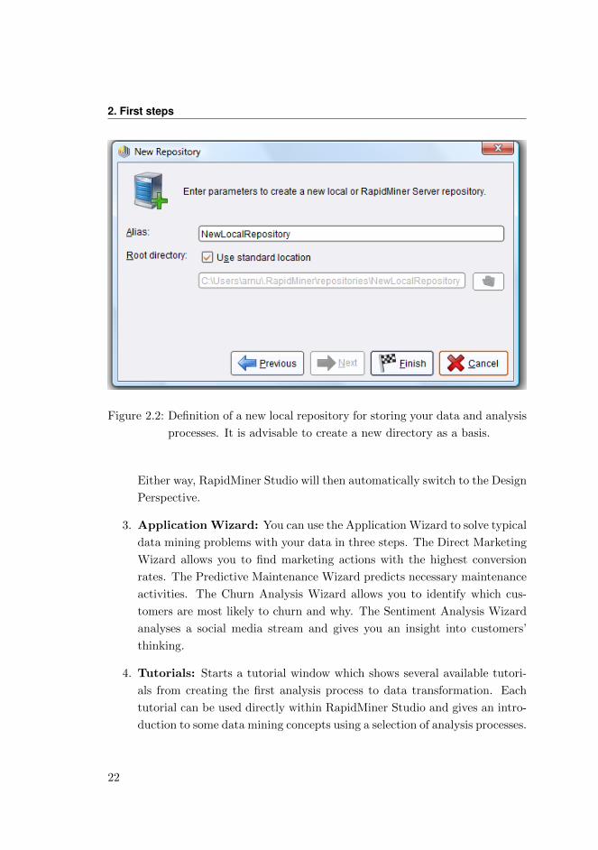
2. First steps
Figure 2.2: Definition of a new local repository for storing your data and analysis
processes. It is advisable to create a new directory as a basis.
Either way, RapidMiner Studio will then automatically switch to the Design
Perspective.
3. Application Wizard: You can use the Application Wizard to solve typical
data mining problems with your data in three steps. The Direct Marketing
Wizard allows you to find marketing actions with the highest conversion
rates. The Predictive Maintenance Wizard predicts necessary maintenance
activities. The Churn Analysis Wizard allows you to identify which cus-
tomers are most likely to churn and why. The Sentiment Analysis Wizard
analyses a social media stream and gives you an insight into customers’
thinking.
4. Tutorials: Starts a tutorial window which shows several available tutori-
als from creating the first analysis process to data transformation. Each
tutorial can be used directly within RapidMiner Studio and gives an intro-
duction to some data mining concepts using a selection of analysis processes.
22
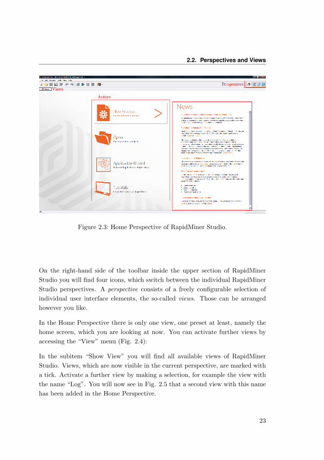
2.2. Perspectives and Views
Figure 2.3: Home Perspective of RapidMiner Studio.
On the right-hand side of the toolbar inside the upper section of RapidMiner
Studio you will find four icons, which switch between the individual RapidMiner
Studio perspectives. A perspective consists of a freely configurable selection of
individual user interface elements, the so-called views. Those can be arranged
however you like.
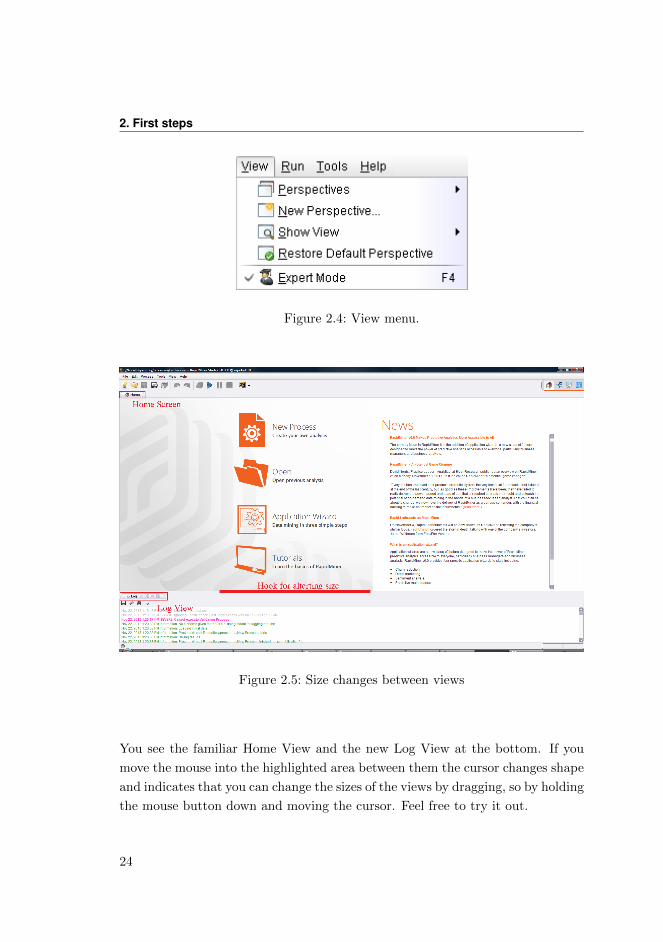
In the Home Perspective there is only one view, one preset at least, namely the
home screen, which you are looking at now. You can activate further views by
accessing the “View” menu (Fig. 2.4):
In the subitem “Show View” you will find all available views of RapidMiner
Studio. Views, which are now visible in the current perspective, are marked with
a tick. Activate a further view by making a selection, for example the view with
the name “Log”. You will now see in Fig. 2.5 that a second view with this name
has been added in the Home Perspective.
23
2. First steps
Figure 2.4: View menu.
Figure 2.5: Size changes between views
You see the familiar Home View and the new Log View at the bottom. If you
move the mouse into the highlighted area between them the cursor changes shape
and indicates that you can change the sizes of the views by dragging, so by holding
the mouse button down and moving the cursor. Feel free to try it out.
24
2.2. Perspectives and Views
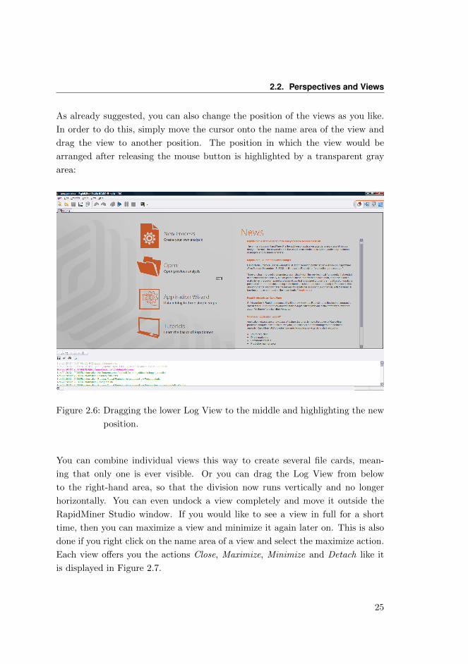
As already suggested, you can also change the position of the views as you like.
In order to do this, simply move the cursor onto the name area of the view and
drag the view to another position. The position in which the view would be
arranged after releasing the mouse button is highlighted by a transparent gray
area:
Figure 2.6: Dragging the lower Log View to the middle and highlighting the new
position.
You can combine individual views this way to create several file cards, mean-
ing that only one is ever visible. Or you can drag the Log View from below
to the right-hand area, so that the division now runs vertically and no longer
horizontally. You can even undock a view completely and move it outside the
RapidMiner Studio window. If you would like to see a view in full for a short
time, then you can maximize a view and minimize it again later on. This is also
done if you right click on the name area of a view and select the maximize action.
Each view offers you the actions Close, Maximize, Minimize and Detach like it
is displayed in Figure 2.7.
25
2. First steps
Figure 2.7: Actions for views
Those actions are possible for all RapidMiner Studio views among others. The
other actions should be self-explanatory:
1. Close: Closes the view in the current perspective. You can re-open the
view in the current or another perspective via the menu “View” – “Show
View”.
2. Maximize: Maximizes the view in the current perspective.
3. Minimize: Minimizes the view in the current perspective. The view is
displayed on the left-hand side of the perspective and can be maximized
again or looked at briefly from there.
4. Detach: Detaches the view from the current perspective and shows it within
its own window, which can be moved to wherever you want.
Now have a little go at arranging the two views in different ways. Sometimes
a little practice is required in order to drop the views in exactly the desired
place. It is worthwhile experimenting a little with the arrangements however,
because other settings may make your work far more efficient depending on screen
resolution and personal preferences.
Sometimes you may inadvertently delete a view or the perspective is uninten-
tionally moved into particularly unfavourable positions. In this case the “View”
menu can help, because apart from the possibility of reopening closed views via
“Show View”, the original state can also be recovered at any time via “Restore
Default Perspective”.
Additionally, you have the option of saving your own perspectives under a freely
selectable name with the action “New Perspective” (Fig. 2.4). You can switch
between the saved and pre-defined perspectives either in the “View” menu or on
the right side of the toolbar.
26
2.3. Design Perspective
2.3 Design Perspective
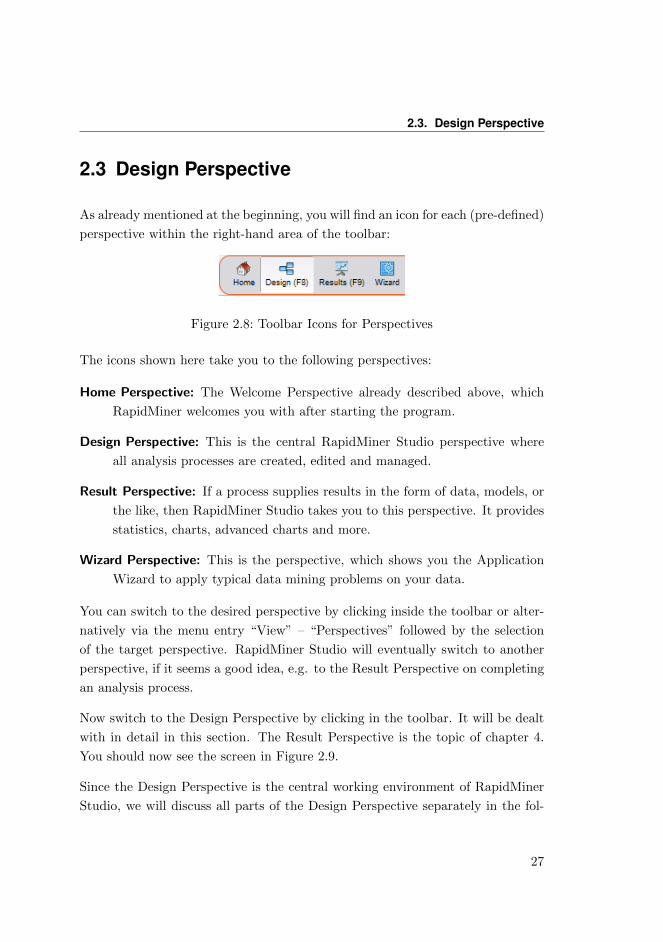
As already mentioned at the beginning, you will find an icon for each (pre-defined)
perspective within the right-hand area of the toolbar:
Figure 2.8: Toolbar Icons for Perspectives
The icons shown here take you to the following perspectives:
Home Perspective: The Welcome Perspective already described above, which
RapidMiner welcomes you with after starting the program.
Design Perspective: This is the central RapidMiner Studio perspective where
all analysis processes are created, edited and managed.
Result Perspective: If a process supplies results in the form of data, models, or
the like, then RapidMiner Studio takes you to this perspective. It provides
statistics, charts, advanced charts and more.
Wizard Perspective: This is the perspective, which shows you the Application
Wizard to apply typical data mining problems on your data.
You can switch to the desired perspective by clicking inside the toolbar or alter-
natively via the menu entry “View” – “Perspectives” followed by the selection
of the target perspective. RapidMiner Studio will eventually switch to another
perspective, if it seems a good idea, e.g. to the Result Perspective on completing
an analysis process.
Now switch to the Design Perspective by clicking in the toolbar. It will be dealt
with in detail in this section. The Result Perspective is the topic of chapter 4.
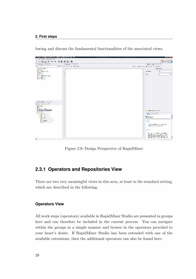
You should now see the screen in Figure 2.9.
Since the Design Perspective is the central working environment of RapidMiner
Studio, we will discuss all parts of the Design Perspective separately in the fol-
27
2. First steps
lowing and discuss the fundamental functionalities of the associated views.
Figure 2.9: Design Perspective of RapidMiner
2.3.1 Operators and Repositories View
There are two very meaningful views in this area, at least in the standard setting,
which are described in the following.
Operators View
All work steps (operators) available in RapidMiner Studio are presented in groups
here and can therefore be included in the current process. You can navigate
within the groups in a simple manner and browse in the operators provided to
your heart’s desire. If RapidMiner Studio has been extended with one of the
available extensions, then the additional operators can also be found here.
28
2.3. Design Perspective
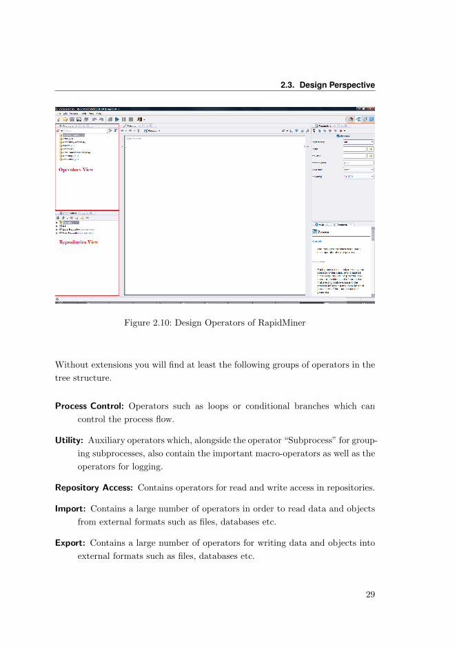
Figure 2.10: Design Operators of RapidMiner
Without extensions you will find at least the following groups of operators in the
tree structure.
Process Control: Operators such as loops or conditional branches which can
control the process flow.
Utility: Auxiliary operators which, alongside the operator “Subprocess” for group-
ing subprocesses, also contain the important macro-operators as well as the
operators for logging.
Repository Access: Contains operators for read and write access in repositories.
Import: Contains a large number of operators in order to read data and objects
from external formats such as files, databases etc.
Export: Contains a large number of operators for writing data and objects into
external formats such as files, databases etc.
29
2. First steps
Data Transformation: Probably the most important group in the analysis in
terms of size and relevance. All operators are located here for transforming
both data and meta data.
Modeling: Contains the actual data mining process such as classification meth-
ods, regression methods, clustering, weightings, methods for association
rules, correlation and similarity analyses as well as operators, in order to
apply the generated models to new data sets.
Evaluation: Operators which can compute the quality of a model and thus for
new data e.g. cross-validations, bootstrapping etc.
You can select operators within the Operators View and add them in the desired
place in the process by drag and drop. You connect the operators by drawing a
line between the output and input ports of the operators. You have the choice
whether you want the operators to be connected automatically, when inserted.
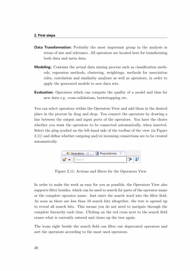
Select the plug symbol on the left-hand side of the toolbar of the view (in Figure
2.11) and define whether outgoing and/or incoming connections are to be created
automatically.
Figure 2.11: Actions and filters for the Operators View
In order to make the work as easy for you as possible, the Operators View also
supports filter besides, which can be used to search for parts of the operator name
or the complete operator name. Just enter the search word into the filter field.
As soon as there are less than 10 search hits altogether, the tree is opened up
to reveal all search hits. This means you do not need to navigate through the
complete hierarchy each time. Clicking on the red cross next to the search field
erases what is currently entered and closes up the tree again.
The icons right beside the search field can filter out deprecated operators and
sort the operators according to the most used operators.
30

2.3. Design Perspective
Tip: Professionals will know the names of the necessary operators more and more
frequently as time goes on. Apart from the search for the (complete) name, the
search field also supports a search based on the initial letters (so-called camel case
search). Just try “REx” for “Read Excel” or “DN” for “Date to Nominal” and
“Date to Numerical” – this speeds up the search enormously.
Repositories View
The repository is a central component of RapidMiner Studio which was intro-
duced in Version 5. It is used for the management and structuring of your anal-
ysis processes into projects and at the same time as both a source of data as well
as of the associated meta data. In the coming chapters we will give a detailed
description of how to use the repository, so we shall just say the following at this
stage.
Warning: Since the majority of the RapidMiner Studio supports make use of meta
data for the process design, we strongly recommend you to use the RapidMiner
repository, since otherwise (for example in the case of data being directly read from
files or databases) the meta data will not be available, meaning that numerous
supports will not be offered.
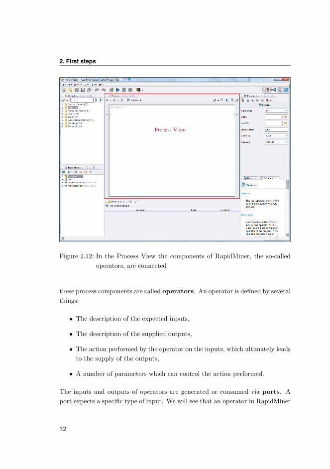
2.3.2 Process View
The Process View (Fig. 2.12) shows the individual steps within the analysis
process as well as their interconnections. New steps can be added to the current
process in several ways. Connections between these steps can be defined and
detached again. Finally, it is even possible to define the order of the steps in this
perspective. The next sections show you how to use the Process View.
2.3.3 Operators and Processes
Working with RapidMiner Studio fundamentally consists in defining analysis pro-
cesses by indicating a succession of individual work steps. In RapidMiner Studio,
31
2. First steps
Figure 2.12: In the Process View the components of RapidMiner, the so-called
operators, are connected
these process components are called operators. An operator is defined by several
things:
• The description of the expected inputs,
• The description of the supplied outputs,
• The action performed by the operator on the inputs, which ultimately leads
to the supply of the outputs,
• A number of parameters which can control the action performed.
The inputs and outputs of operators are generated or consumed via ports. A
port expects a specific type of input. We will see that an operator in RapidMiner
32
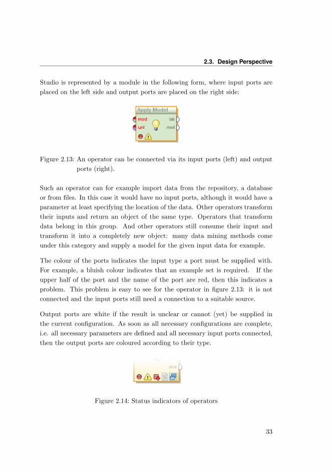
2.3. Design Perspective
Studio is represented by a module in the following form, where input ports are
placed on the left side and output ports are placed on the right side:
Figure 2.13: An operator can be connected via its input ports (left) and output
ports (right).
Such an operator can for example import data from the repository, a database
or from files. In this case it would have no input ports, although it would have a
parameter at least specifying the location of the data. Other operators transform
their inputs and return an object of the same type. Operators that transform
data belong in this group. And other operators still consume their input and
transform it into a completely new object: many data mining methods come
under this category and supply a model for the given input data for example.
The colour of the ports indicates the input type a port must be supplied with.
For example, a bluish colour indicates that an example set is required. If the
upper half of the port and the name of the port are red, then this indicates a
problem. This problem is easy to see for the operator in figure 2.13: it is not
connected and the input ports still need a connection to a suitable source.
Output ports are white if the result is unclear or cannot (yet) be supplied in
the current configuration. As soon as all necessary configurations are complete,
i.e. all necessary parameters are defined and all necessary input ports connected,
then the output ports are coloured according to their type.
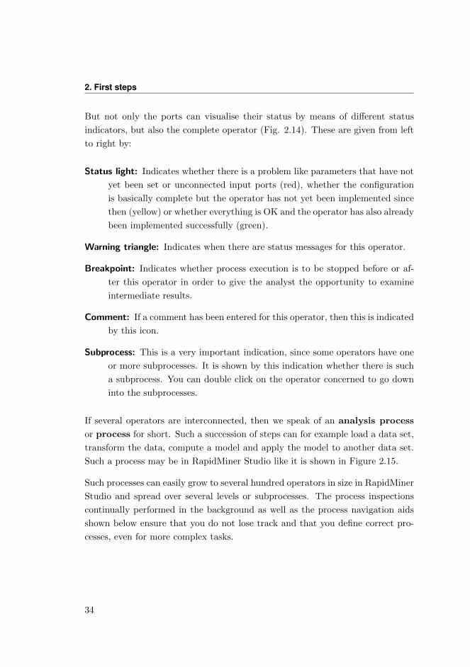
Figure 2.14: Status indicators of operators
33
2. First steps
But not only the ports can visualise their status by means of different status
indicators, but also the complete operator (Fig. 2.14). These are given from left
to right by:
Status light: Indicates whether there is a problem like parameters that have not
yet been set or unconnected input ports (red), whether the configuration
is basically complete but the operator has not yet been implemented since
then (yellow) or whether everything is OK and the operator has also already
been implemented successfully (green).
Warning triangle: Indicates when there are status messages for this operator.
Breakpoint: Indicates whether process execution is to be stopped before or af-
ter this operator in order to give the analyst the opportunity to examine
intermediate results.
Comment: If a comment has been entered for this operator, then this is indicated
by this icon.
Subprocess: This is a very important indication, since some operators have one
or more subprocesses. It is shown by this indication whether there is such
a subprocess. You can double click on the operator concerned to go down
into the subprocesses.
If several operators are interconnected, then we speak of an analysis process
or process for short. Such a succession of steps can for example load a data set,
transform the data, compute a model and apply the model to another data set.
Such a process may be in RapidMiner Studio like it is shown in Figure 2.15.
Such processes can easily grow to several hundred operators in size in RapidMiner
Studio and spread over several levels or subprocesses. The process inspections
continually performed in the background as well as the process navigation aids
shown below ensure that you do not lose track and that you define correct pro-
cesses, even for more complex tasks.
34

2.3. Design Perspective
Figure 2.15: An analysis process consisting of several operators. The colour cod-
ing of the data flows shows the type of object passed on.
Inserting Operators
You can insert new operators into the process in different ways. Here are the
details of the different ways:
• Via drag&drop from the Operators View as described above,
• Via double click on an operator in the Operators View,
• Via dialog which is opened by the menu entry “Edit” – “ New Operator. . . ”
(Ctrl-I),
• Via context menu in a free area of the white process area and there via the
submenu“New Operator” and the selection of an operator.
In each case new operators are, depending on the setting in the Operators View,
either automatically connected with suitable operators, or the connections have
to be made or corrected manually by the user.
35
2. First steps
Connecting Operators
After you have inserted new operators, you can interconnect the operators in-
serted. There are basically three ways available to you, which will be described
in the following.
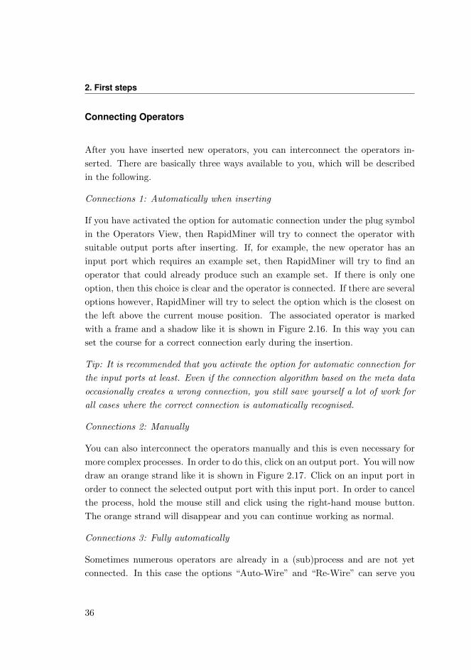
Connections 1: Automatically when inserting
If you have activated the option for automatic connection under the plug symbol
in the Operators View, then RapidMiner will try to connect the operator with
suitable output ports after inserting. If, for example, the new operator has an
input port which requires an example set, then RapidMiner will try to find an
operator that could already produce such an example set. If there is only one
option, then this choice is clear and the operator is connected. If there are several
options however, RapidMiner will try to select the option which is the closest on
the left above the current mouse position. The associated operator is marked
with a frame and a shadow like it is shown in Figure 2.16. In this way you can
set the course for a correct connection early during the insertion.
Tip: It is recommended that you activate the option for automatic connection for
the input ports at least. Even if the connection algorithm based on the meta data
occasionally creates a wrong connection, you still save yourself a lot of work for
all cases where the correct connection is automatically recognised.
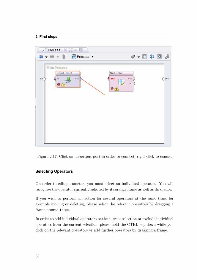
Connections 2: Manually
You can also interconnect the operators manually and this is even necessary for
more complex processes. In order to do this, click on an output port. You will now
draw an orange strand like it is shown in Figure 2.17. Click on an input port in
order to connect the selected output port with this input port. In order to cancel
the process, hold the mouse still and click using the right-hand mouse button.
The orange strand will disappear and you can continue working as normal.
Connections 3: Fully automatically
Sometimes numerous operators are already in a (sub)process and are not yet
connected. In this case the options “Auto-Wire” and “Re-Wire” can serve you
36
2.3. Design Perspective
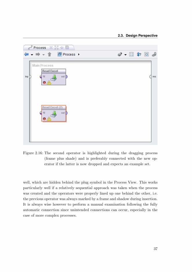
Figure 2.16: The second operator is highlighted during the dragging process
(frame plus shade) and is preferably connected with the new op-
erator if the latter is now dropped and expects an example set.
well, which are hidden behind the plug symbol in the Process View. This works
particularly well if a relatively sequential approach was taken when the process
was created and the operators were properly lined up one behind the other, i.e.
the previous operator was always marked by a frame and shadow during insertion.
It is always wise however to perform a manual examination following the fully
automatic connection since unintended connections can occur, especially in the
case of more complex processes.
37
2. First steps
Figure 2.17: Click on an output port in order to connect, right click to cancel.
Selecting Operators
On order to edit parameters you must select an individual operator. You will
recognise the operator currently selected by its orange frame as well as its shadow.
If you wish to perform an action for several operators at the same time, for
example moving or deleting, please select the relevant operators by dragging a
frame around these.
In order to add individual operators to the current selection or exclude individual
operators from the current selection, please hold the CTRL key down while you
click on the relevant operators or add further operators by dragging a frame.
38
2.3. Design Perspective
Moving Operators
Select one or more operators as described above. Now move the cursor onto one
of the selected operators and drag the mouse while holding down the button. All
selected operators will now be moved to a new place depending on where you
move the mouse.
If, in the course of this movement, you reach the edge of the white area, then
this will be automatically enlarged accordingly. If you should reach the edge of
the visible area, then this will also be moved along automatically.
Copying Operators
Select one or more operators as described above. Now press Ctrl+C to copy the
selected operators and press Ctrl+V to paste them. All selected operators will
now be placed to a new place next to the original operators, where you can move
them further.
Deleting Operators
Select one or more operators as described above. You can now delete the selected
operators by
• Pressing the DELETE key,
• Selecting the action “Delete” in the context menu of one of the selected
operators,
• By means of the menu entry “Edit” – “Delete”.
Deleting Connections
Connections can be deleted by clicking on one of the two ports while pressing the
ALT key at the same time. Alternatively, you can also delete a connection via
39
2. First steps
the context menu of the ports concerned.
Navigating Within the Process
If we look at the toolbar of the Process View, then we can see that we have
only made use of one action so far. In this section we will discuss the following
four elements on the left side of the toolbar: the arrow pointing left, the arrow
pointing right, the arrow pointing upwards and the navigation bar (breadcrumb).
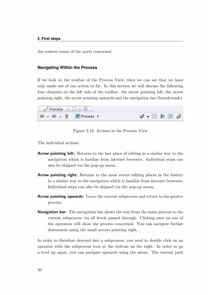
Figure 2.18: Actions in the Process View
The individual actions:
Arrow pointing left: Returns to the last place of editing in a similar way to the
navigation which is familiar from internet browsers. Individual steps can
also be skipped via the pop-up menu.
Arrow pointing right: Returns to the most recent editing places in the history
in a similar way to the navigation which is familiar from internet browsers.
Individual steps can also be skipped via the pop-up menu.
Arrow pointing upwards: Leave the current subprocess and return to the greater
process.
Navigation bar: The navigation bar shows the way from the main process to the
current subprocess via all levels passed through. Clicking once on one of
the operators will show the process concerned. You can navigate further
downwards using the small arrows pointing right.
In order to therefore descend into a subprocess, you need to double click on an
operator with the subprocess icon at the bottom on the right. In order to go
a level up again, you can navigate upwards using the arrow. The current path
40
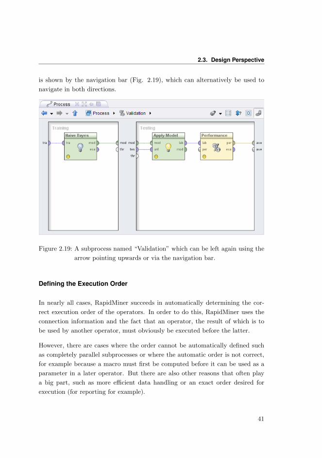
2.3. Design Perspective
is shown by the navigation bar (Fig. 2.19), which can alternatively be used to
navigate in both directions.
Figure 2.19: A subprocess named “Validation” which can be left again using the
arrow pointing upwards or via the navigation bar.
Defining the Execution Order
In nearly all cases, RapidMiner succeeds in automatically determining the cor-
rect execution order of the operators. In order to do this, RapidMiner uses the
connection information and the fact that an operator, the result of which is to
be used by another operator, must obviously be executed before the latter.
However, there are cases where the order cannot be automatically defined such
as completely parallel subprocesses or where the automatic order is not correct,
for example because a macro must first be computed before it can be used as a
parameter in a later operator. But there are also other reasons that often play
a big part, such as more efficient data handling or an exact order desired for
execution (for reporting for example).
41
2. First steps
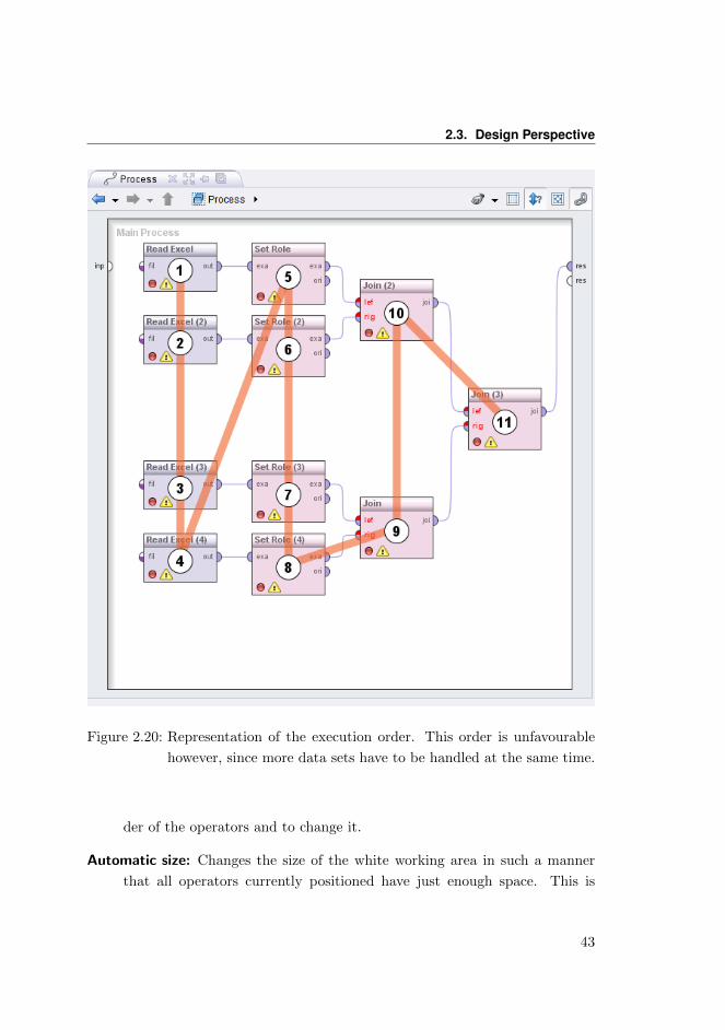
For this purpose, RapidMiner offers an elegant method for indicating the order
of the operators and even for editing the execution order comfortably. Please
click on icon with the double arrow pointing upwards and downwards with the
question mark in the toolbar of the Process View (Fig. 2.18) and the process view
shows the order definition of the operators. Instead of the icon for each operator,
the number of its execution will now be shown. The transparent orange line
connects the operators in this order, as shown in Figure 2.20.
To change such an execution order, you can click anywhere on an operator to
select it. The path leading to this operator can now not be changed, but clicking
again on another operator will attempt to change the order in such a way that
the second operator is executed as soon as possible after the first. While you
move the mouse over the remaining operators, you will see the current choice in
orange up to this operator and in grey starting from this operator. A choice that
is not possible is symbolised by a red number. You can cancel a current selection
by right-clicking. In this way you can, as shown in Fig. 2.21, change the order
of the process described above to the following with only a few clicks.
2.3.4 Further Options of the Process View
After having discussed nearly all options of this central element of the RapidMiner
Design Perspective, we will now describe the remaining actions in the toolbar,
which can be seen in Figure 2.18, as well as further possibilities of the Process
View.
The five icons on the right-hand side of the Process View toolbar perform the
following actions:
Auto-wire and Re-wire connections The plug symbol allows to auto-wire and
re-wire the connections between operators.
Automatic arrangement: Rearranges all operators of the current process accord-
ing to the connections and the current execution order.
Show and alter execution order This action allows you to see the execution or-
42
2.3. Design Perspective
Figure 2.20: Representation of the execution order. This order is unfavourable
however, since more data sets have to be handled at the same time.
der of the operators and to change it.
Automatic size: Changes the size of the white working area in such a manner
that all operators currently positioned have just enough space. This is
43
2. First steps
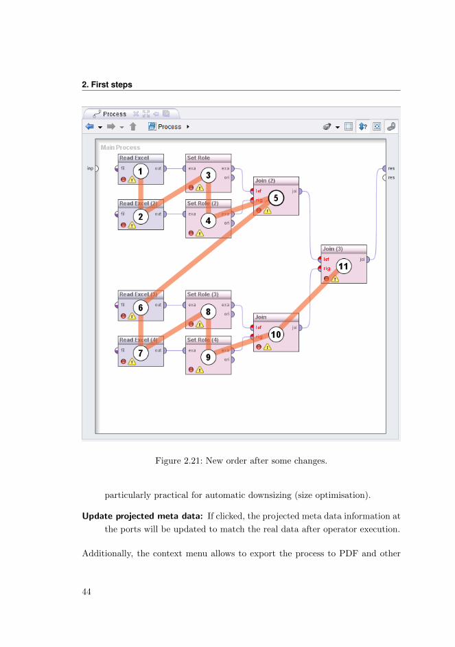
Figure 2.21: New order after some changes.
particularly practical for automatic downsizing (size optimisation).
Update projected meta data: If clicked, the projected meta data information at
the ports will be updated to match the real data after operator execution.
Additionally, the context menu allows to export the process to PDF and other
44
2.3. Design Perspective
formats and to print it.
2.3.5 Parameters View
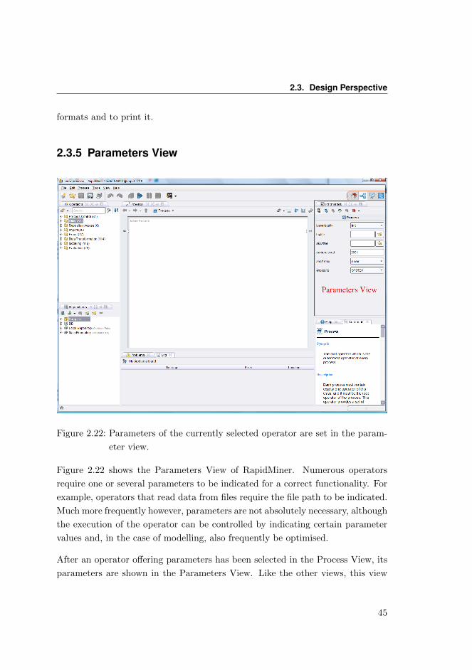
Figure 2.22: Parameters of the currently selected operator are set in the param-
eter view.
Figure 2.22 shows the Parameters View of RapidMiner. Numerous operators
require one or several parameters to be indicated for a correct functionality. For
example, operators that read data from files require the file path to be indicated.
Much more frequently however, parameters are not absolutely necessary, although
the execution of the operator can be controlled by indicating certain parameter
values and, in the case of modelling, also frequently be optimised.
After an operator offering parameters has been selected in the Process View, its
parameters are shown in the Parameters View. Like the other views, this view
45
2. First steps
also has its own toolbar which is described in the following. Under the toolbar
you will find the icon and name of the operator currently selected followed by
the actual parameters. Bold font means that the parameter must absolutely be
defined and has no default value. Italic font means that the parameter is classified
as an expert parameter and should not necessarily be changed by beginners to
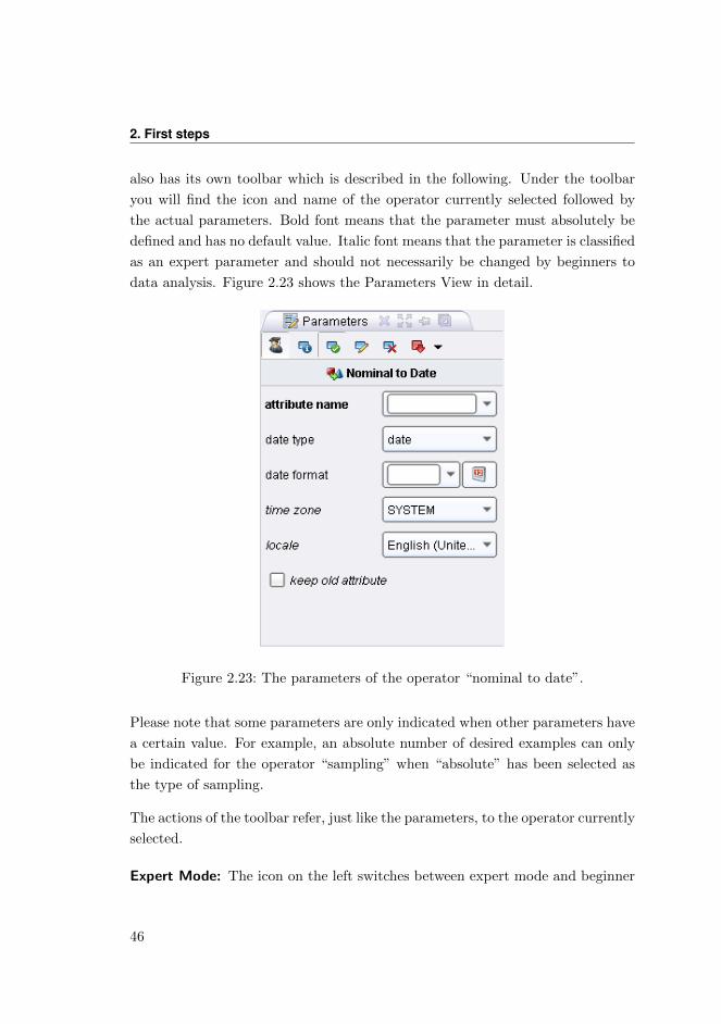
data analysis. Figure 2.23 shows the Parameters View in detail.
Figure 2.23: The parameters of the operator “nominal to date”.
Please note that some parameters are only indicated when other parameters have
a certain value. For example, an absolute number of desired examples can only
be indicated for the operator “sampling” when “absolute” has been selected as
the type of sampling.
The actions of the toolbar refer, just like the parameters, to the operator currently
selected.
Expert Mode: The icon on the left switches between expert mode and beginner
46
2.3. Design Perspective
mode. Only in the expert mode are all parameters shown; in the beginner
mode the parameters classified as expert parameters are not shown.
Operator Info: Display of some fundamental information about this operator
such as expected inputs or a description. This dialog is also displayed by
pressing F1 after selection, via the context menu in the Process View as
well as via the menu entry “Edit” – “Show Operator Info. . . ”.
Enable/Disable: Operators can be (temporarily) deactivated. Their connections
are detached and they are no longer executed. Deactivated operators are
shown in gray. Operators can also be (de)activated within their context
menu in the Process View as well as via the menu entry “Edit” – “Enable
Operator”.
Rename: One of the ways to rename an operator. Further ways are pressing F2
after selection, selecting “Rename” in the context menu of the operator in
the Process View as well as the menu entry “Edit” – “Rename”.
Delete: One of the ways to delete an operator. Further ways are pressing
DELETE after selection, selecting “Delete” in the context menu of the
operator in the Process View as well as the menu entry “Edit” – “Delete”.
Toggle Breakpoints: Breakpoints can be set here both before and after the exe-
cution of the operator, where the process execution stops and intermediate
results can be examined. There is also this possibility in the context menu
of the operator in the Process View as well as in the “Edit” menu. A break-
point after operator execution can also be activated and deactivated with
F7.
2.3.6 Help and Comment View
Help View
Each time you select an operator in the Operators View or in the Process View,
the help window within the Help View shows a description of this operator. This
47
2. First steps
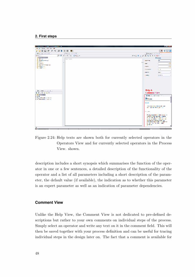
Figure 2.24: Help texts are shown both for currently selected operators in the
Operators View and for currently selected operators in the Process
View. shown.
description includes a short synopsis which summarises the function of the oper-
ator in one or a few sentences, a detailed description of the functionality of the
operator and a list of all parameters including a short description of the param-
eter, the default value (if available), the indication as to whether this parameter
is an expert parameter as well as an indication of parameter dependencies.
Comment View
Unlike the Help View, the Comment View is not dedicated to pre-defined de-
scriptions but rather to your own comments on individual steps of the process.
Simply select an operator and write any text on it in the comment field. This will
then be saved together with your process definition and can be useful for tracing
individual steps in the design later on. The fact that a comment is available for
48
2.3. Design Perspective
an operator is indicated by a small text icon at the lower edge of the operator.
2.3.7 Overview View
Particularly in the case of extensive processes, the white work area will no longer
be sufficient and will be enlarged either via the context menu of the Process
View, by means of the key combinations of Ctrl and the arrow pointing left,
right, upwards and downwards or simply by dragging an operator to the edge.
In this case however, the entire work area will no longer be visible at the same
time and navigation within the process will be made more difficult. In order to
improve the overview and provide a comfortable way of navigating at the same
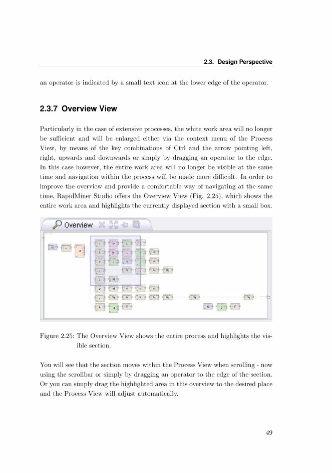
time, RapidMiner Studio offers the Overview View (Fig. 2.25), which shows the
entire work area and highlights the currently displayed section with a small box.
Figure 2.25: The Overview View shows the entire process and highlights the vis-
ible section.
You will see that the section moves within the Process View when scrolling - now
using the scrollbar or simply by dragging an operator to the edge of the section.
Or you can simply drag the highlighted area in this overview to the desired place
and the Process View will adjust automatically.
49
2. First steps
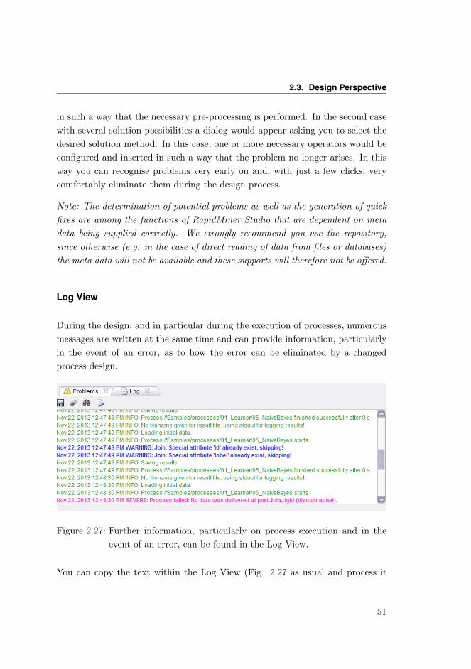
2.3.8 Problems and Log View
Problems View
A further very central element and valuable source of help during the design of
your analysis processes is the Problems View. Any warnings and error messages
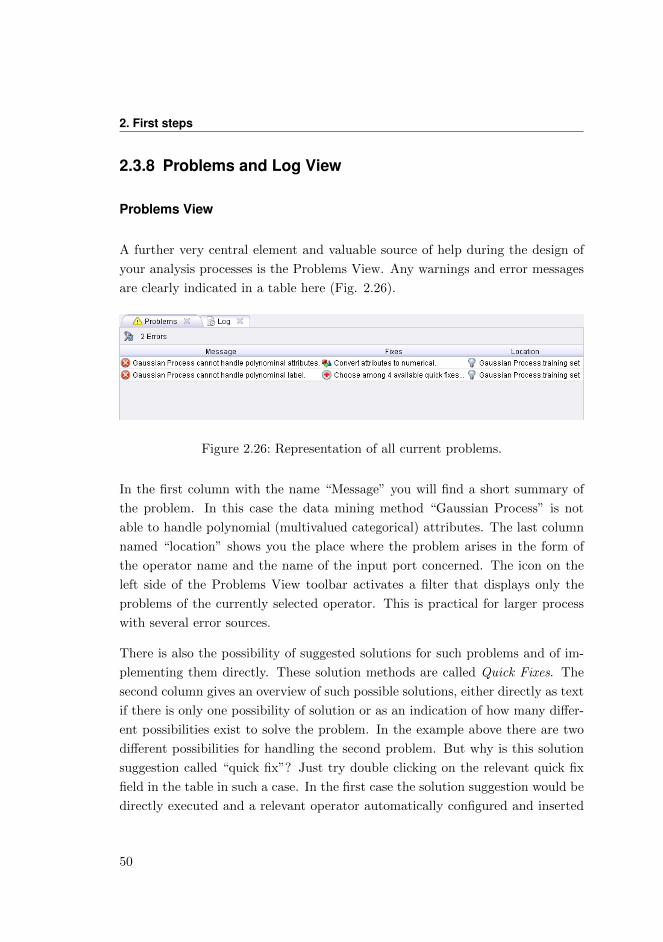
are clearly indicated in a table here (Fig. 2.26).
Figure 2.26: Representation of all current problems.
In the first column with the name “Message” you will find a short summary of
the problem. In this case the data mining method “Gaussian Process” is not
able to handle polynomial (multivalued categorical) attributes. The last column
named “location” shows you the place where the problem arises in the form of
the operator name and the name of the input port concerned. The icon on the
left side of the Problems View toolbar activates a filter that displays only the
problems of the currently selected operator. This is practical for larger process
with several error sources.
There is also the possibility of suggested solutions for such problems and of im-
plementing them directly. These solution methods are called Quick Fixes. The
second column gives an overview of such possible solutions, either directly as text
if there is only one possibility of solution or as an indication of how many differ-
ent possibilities exist to solve the problem. In the example above there are two
different possibilities for handling the second problem. But why is this solution
suggestion called “quick fix”? Just try double clicking on the relevant quick fix
field in the table in such a case. In the first case the solution suggestion would be
directly executed and a relevant operator automatically configured and inserted
50
2.3. Design Perspective
in such a way that the necessary pre-processing is performed. In the second case
with several solution possibilities a dialog would appear asking you to select the
desired solution method. In this case, one or more necessary operators would be
configured and inserted in such a way that the problem no longer arises. In this
way you can recognise problems very early on and, with just a few clicks, very
comfortably eliminate them during the design process.
Note: The determination of potential problems as well as the generation of quick
fixes are among the functions of RapidMiner Studio that are dependent on meta
data being supplied correctly. We strongly recommend you use the repository,
since otherwise (e.g. in the case of direct reading of data from files or databases)
the meta data will not be available and these supports will therefore not be offered.
Log View
During the design, and in particular during the execution of processes, numerous
messages are written at the same time and can provide information, particularly
in the event of an error, as to how the error can be eliminated by a changed
process design.
Figure 2.27: Further information, particularly on process execution and in the
event of an error, can be found in the Log View.
You can copy the text within the Log View (Fig. 2.27 as usual and process it
51

2. First steps
further in other applications. You can also save the text in a file, delete the entire
contents or search through the text using the actions in the toolbar.
52
3 Design ofAnalysis Processes
We became acquainted with the fundamental elements of the graphical user in-
terface of RapidMiner Studio in the last chapter, such as perspectives and views,
and discussed the most important aspects of the Design Perspective of Rapid-
Miner Studio. We would now like to make use of the new possibilities in order
to define and execute an initial simple analysis process. You will soon realise
how practical it is that, with RapidMiner Studio, you do not need to perform
the process again for every change in order to determine the effect of the change.
But more about it later.
3.1 Creating a New Process
Whether you now select the action “New” from the Home Perspective, the “New”
icon on the left side of the main toolbar of RapidMiner Studio or the associated
entry in the “File” menu: A new analysis process is created in each case, which
you can work on in the following.
Tip: We recommend to save the process in your repository, when it is created.
53
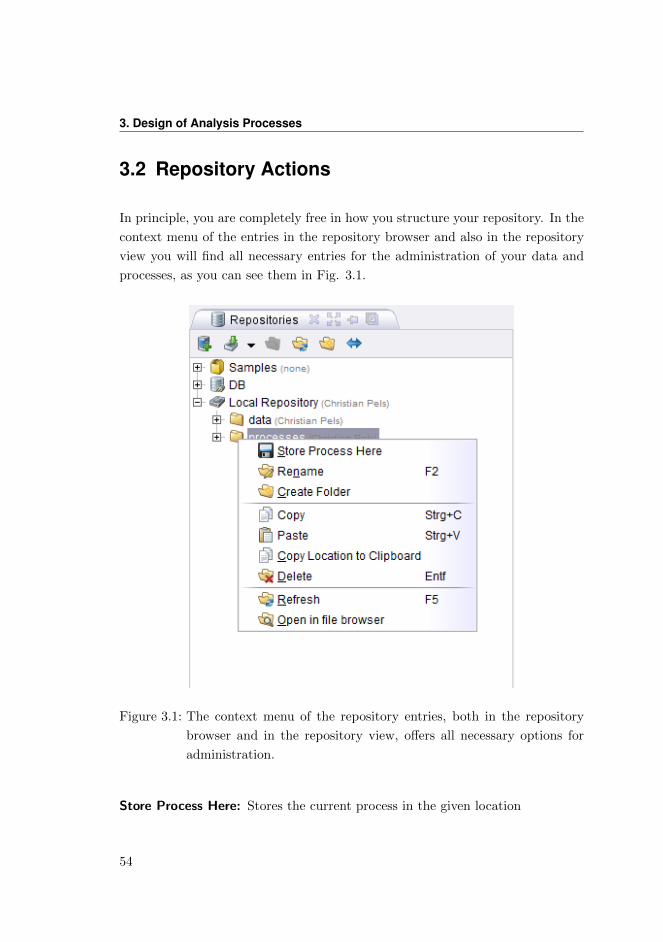
3. Design of Analysis Processes
3.2 Repository Actions
In principle, you are completely free in how you structure your repository. In the
context menu of the entries in the repository browser and also in the repository
view you will find all necessary entries for the administration of your data and
processes, as you can see them in Fig. 3.1.
Figure 3.1: The context menu of the repository entries, both in the repository
browser and in the repository view, offers all necessary options for
administration.
Store Process Here: Stores the current process in the given location
54
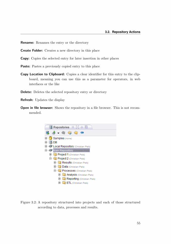
3.2. Repository Actions
Rename: Renames the entry or the directory
Create Folder: Creates a new directory in this place
Copy: Copies the selected entry for later insertion in other places
Paste: Pastes a previously copied entry to this place
Copy Location to Clipboard: Copies a clear identifier for this entry to the clip-
board, meaning you can use this as a parameter for operators, in web
interfaces or the like
Delete: Deletes the selected repository entry or directory
Refresh: Updates the display
Open in file browser: Shows the repository in a file browser. This is not recom-
mended.
Figure 3.2: A repository structured into projects and each of those structured
according to data, processes and results.
55
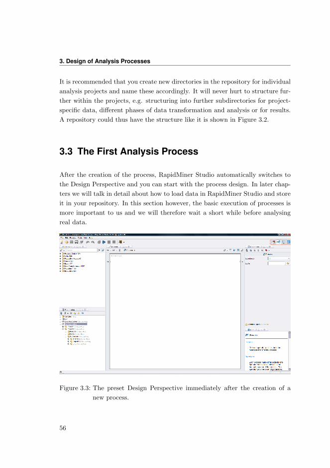
3. Design of Analysis Processes
It is recommended that you create new directories in the repository for individual
analysis projects and name these accordingly. It will never hurt to structure fur-
ther within the projects, e.g. structuring into further subdirectories for project-
specific data, different phases of data transformation and analysis or for results.
A repository could thus have the structure like it is shown in Figure 3.2.
3.3 The First Analysis Process
After the creation of the process, RapidMiner Studio automatically switches to
the Design Perspective and you can start with the process design. In later chap-
ters we will talk in detail about how to load data in RapidMiner Studio and store
it in your repository. In this section however, the basic execution of processes is
more important to us and we will therefore wait a short while before analysing
real data.
Figure 3.3: The preset Design Perspective immediately after the creation of a
new process.
56
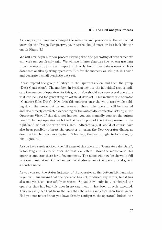
3.3. The First Analysis Process
As long as you have not changed the selection and positions of the individual
views for the Design Perspective, your screen should more or less look like the
one in Figure 3.3.
We will now begin our new process starting with the generating of data which we
can work on. As already said: We will see in later chapters how we can use data
from the repository or even import it directly from other data sources such as
databases or files by using operators. But for the moment we will put this aside
and generate a small synthetic data set.
Please expand the group “Utility” in the Operators View and then the group
“Data Generation”. The numbers in brackets next to the individual groups indi-
cate the number of operators for this group. You should now see several operators
that can be used for generating an artificial data set. This includes the operator
“Generate Sales Data”. Now drag this operator onto the white area while hold-
ing down the mouse button and release it there. The operator will be inserted
and also directly connected depending on the automatic connection setting in the
Operators View. If this does not happen, you can manually connect the output
port of the new operator with the first result port of the entire process on the
right-hand side of the white work area. Alternatively, it would of course have
also been possible to insert the operator by using the New Operator dialog, as
described in the previous chapter. Either way, the result ought to look roughly
like Figure 3.4.
As you have surely noticed, the full name of this operator, “Generate Sales Data”,
is too long and is cut off after the first few letters. Move the mouse onto this
operator and stay there for a few moments. The name will now be shown in full
in a small animation. Of course, you could also rename the operator and give it
a shorter name.
As you can see, the status indicator of the operator at the bottom left-hand side
is yellow. This means that the operator has not produced any errors, but it has
also not yet been successfully executed. So you have only fully configured the
operator thus far, but this does in no way mean it has been directly executed.
You can easily see that from the fact that the status indicator then turns green.
Had you not noticed that you have already configured the operator? Indeed, the
57

3. Design of Analysis Processes
Figure 3.4: An initial and admittedly very simple process, which generates some
data and displays the result in the Result Perspective.
configuration was very simple in this specific case: It was not at all necessary to
set any operator parameter. A red status indicator and entries in the Problems
View would have indicated such a configuration need.
3.3.1 Transforming Meta Data
We will now deal with one of the most fascinating aspects of RapidMiner Studio,
namely the ability to compute the output of an operator or process beforehand
and to even do this during the design time, so without having to load the actual
data or even perform the process. This is made possible by the so-called meta
data transformation of RapidMiner Studio.
Of course, each operator defines the way in which the received input data is
transformed. This is its task at the end of the day. The special thing about
RapidMiner Studio however is that this can not only be done for actual data but
also for the meta data about this data. This is typically much less voluminous
58
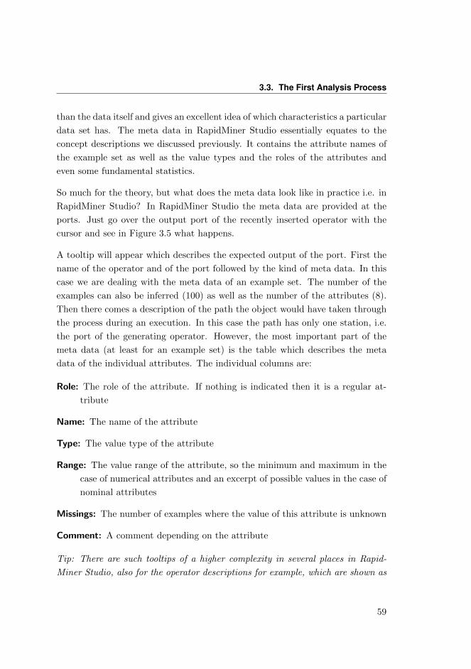
3.3. The First Analysis Process
than the data itself and gives an excellent idea of which characteristics a particular
data set has. The meta data in RapidMiner Studio essentially equates to the
concept descriptions we discussed previously. It contains the attribute names of
the example set as well as the value types and the roles of the attributes and
even some fundamental statistics.
So much for the theory, but what does the meta data look like in practice i.e. in
RapidMiner Studio? In RapidMiner Studio the meta data are provided at the
ports. Just go over the output port of the recently inserted operator with the
cursor and see in Figure 3.5 what happens.
A tooltip will appear which describes the expected output of the port. First the
name of the operator and of the port followed by the kind of meta data. In this
case we are dealing with the meta data of an example set. The number of the
examples can also be inferred (100) as well as the number of the attributes (8).
Then there comes a description of the path the object would have taken through
the process during an execution. In this case the path has only one station, i.e.
the port of the generating operator. However, the most important part of the
meta data (at least for an example set) is the table which describes the meta
data of the individual attributes. The individual columns are:
Role: The role of the attribute. If nothing is indicated then it is a regular at-
tribute
Name: The name of the attribute
Type: The value type of the attribute
Range: The value range of the attribute, so the minimum and maximum in the
case of numerical attributes and an excerpt of possible values in the case of
nominal attributes
Missings: The number of examples where the value of this attribute is unknown
Comment: A comment depending on the attribute
Tip: There are such tooltips of a higher complexity in several places in Rapid-
Miner Studio, also for the operator descriptions for example, which are shown as
59

3. Design of Analysis Processes
Figure 3.5: The meta data of the output port of the operator “Generate Sales
Data”.
a tooltip in the Operators View. You can take time to read the tooltip and also
adjust it in terms of size if you press the key F3 beforehand.
Please note that the meta data can often only represent an estimation and that
an exact indication is not always possible. This is explained by the fact that parts
of the meta data are unknown or can only be indicated inaccurately, e.g. with
60
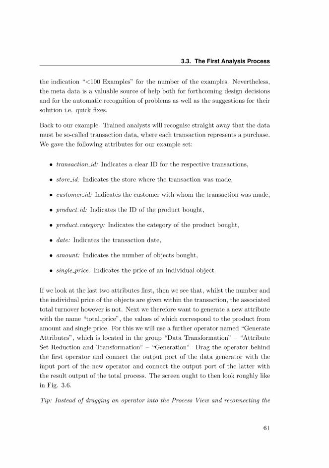
3.3. The First Analysis Process
the indication “<100 Examples” for the number of the examples. Nevertheless,
the meta data is a valuable source of help both for forthcoming design decisions
and for the automatic recognition of problems as well as the suggestions for their
solution i.e. quick fixes.
Back to our example. Trained analysts will recognise straight away that the data
must be so-called transaction data, where each transaction represents a purchase.
We gave the following attributes for our example set:
• transaction id: Indicates a clear ID for the respective transactions,
• store id: Indicates the store where the transaction was made,
• customer id: Indicates the customer with whom the transaction was made,
• product id: Indicates the ID of the product bought,
• product category: Indicates the category of the product bought,
• date: Indicates the transaction date,
• amount: Indicates the number of objects bought,
• single price: Indicates the price of an individual object.
If we look at the last two attributes first, then we see that, whilst the number and
the individual price of the objects are given within the transaction, the associated
total turnover however is not. Next we therefore want to generate a new attribute
with the name “total price”, the values of which correspond to the product from
amount and single price. For this we will use a further operator named “Generate
Attributes”, which is located in the group “Data Transformation” – “Attribute
Set Reduction and Transformation” – “Generation”. Drag the operator behind
the first operator and connect the output port of the data generator with the
input port of the new operator and connect the output port of the latter with
the result output of the total process. The screen ought to then look roughly like
in Fig. 3.6.
Tip: Instead of dragging an operator into the Process View and reconnecting the
61
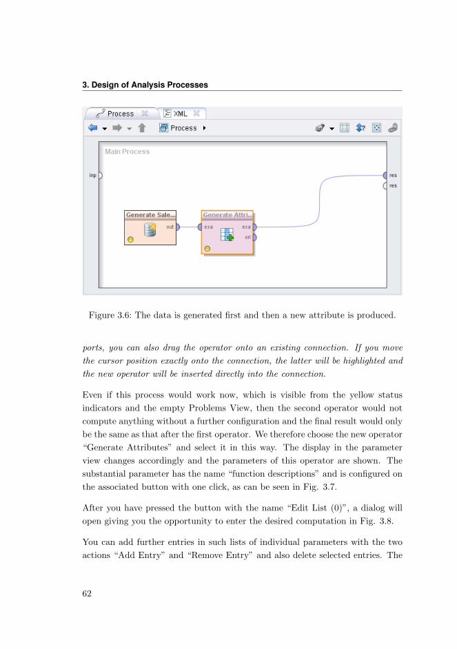
3. Design of Analysis Processes
Figure 3.6: The data is generated first and then a new attribute is produced.
ports, you can also drag the operator onto an existing connection. If you move
the cursor position exactly onto the connection, the latter will be highlighted and
the new operator will be inserted directly into the connection.
Even if this process would work now, which is visible from the yellow status
indicators and the empty Problems View, then the second operator would not
compute anything without a further configuration and the final result would only
be the same as that after the first operator. We therefore choose the new operator
“Generate Attributes” and select it in this way. The display in the parameter
view changes accordingly and the parameters of this operator are shown. The
substantial parameter has the name “function descriptions” and is configured on
the associated button with one click, as can be seen in Fig. 3.7.
After you have pressed the button with the name “Edit List (0)”, a dialog will
open giving you the opportunity to enter the desired computation in Fig. 3.8.
You can add further entries in such lists of individual parameters with the two
actions “Add Entry” and “Remove Entry” and also delete selected entries. The
62
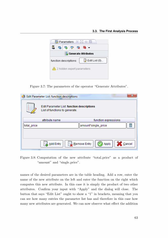
3.3. The First Analysis Process
Figure 3.7: The parameters of the operator “Generate Attributes”.
Figure 3.8: Computation of the new attribute “total price” as a product of
“amount” and “single price”.
names of the desired parameters are in the table heading. Add a row, enter the
name of the new attribute on the left and enter the function on the right which
computes this new attribute. In this case it is simply the product of two other
attributes. Confirm your input with “Apply” and the dialog will close. The
button that says “Edit List” ought to show a “1” in brackets, meaning that you
can see how many entries the parameter list has and therefore in this case how
many new attributes are generated. We can now observe what effect the addition
63
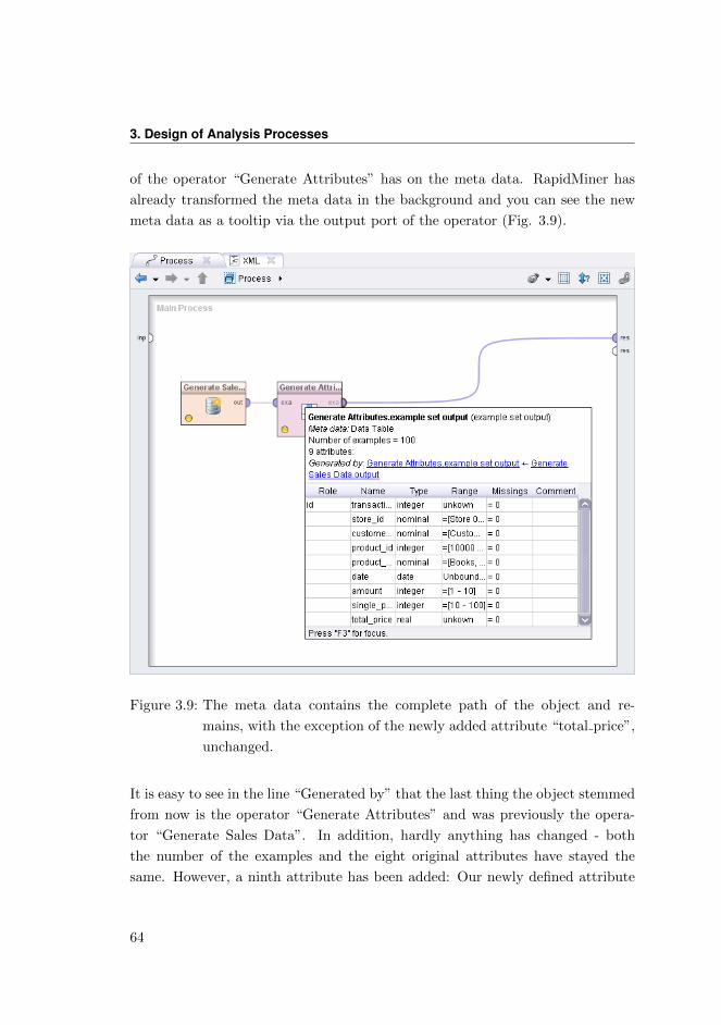
3. Design of Analysis Processes
of the operator “Generate Attributes” has on the meta data. RapidMiner has
already transformed the meta data in the background and you can see the new
meta data as a tooltip via the output port of the operator (Fig. 3.9).
Figure 3.9: The meta data contains the complete path of the object and re-
mains, with the exception of the newly added attribute “total price”,
unchanged.
It is easy to see in the line “Generated by” that the last thing the object stemmed
from now is the operator “Generate Attributes” and was previously the opera-
tor “Generate Sales Data”. In addition, hardly anything has changed - both
the number of the examples and the eight original attributes have stayed the
same. However, a ninth attribute has been added: Our newly defined attribute
64
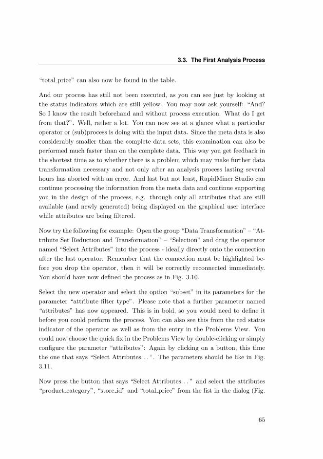
3.3. The First Analysis Process
“total price” can also now be found in the table.
And our process has still not been executed, as you can see just by looking at
the status indicators which are still yellow. You may now ask yourself: “And?
So I know the result beforehand and without process execution. What do I get
from that?”. Well, rather a lot. You can now see at a glance what a particular
operator or (sub)process is doing with the input data. Since the meta data is also
considerably smaller than the complete data sets, this examination can also be
performed much faster than on the complete data. This way you get feedback in
the shortest time as to whether there is a problem which may make further data
transformation necessary and not only after an analysis process lasting several
hours has aborted with an error. And last but not least, RapidMiner Studio can
continue processing the information from the meta data and continue supporting
you in the design of the process, e.g. through only all attributes that are still
available (and newly generated) being displayed on the graphical user interface
while attributes are being filtered.
Now try the following for example: Open the group “Data Transformation” – “At-
tribute Set Reduction and Transformation” – “Selection” and drag the operator
named “Select Attributes” into the process - ideally directly onto the connection
after the last operator. Remember that the connection must be highlighted be-
fore you drop the operator, then it will be correctly reconnected immediately.
You should have now defined the process as in Fig. 3.10.
Select the new operator and select the option “subset” in its parameters for the
parameter “attribute filter type”. Please note that a further parameter named
“attributes” has now appeared. This is in bold, so you would need to define it
before you could perform the process. You can also see this from the red status
indicator of the operator as well as from the entry in the Problems View. You
could now choose the quick fix in the Problems View by double-clicking or simply
configure the parameter “attributes”: Again by clicking on a button, this time
the one that says “Select Attributes. . . ”. The parameters should be like in Fig.
3.11.
Now press the button that says “Select Attributes. . . ” and select the attributes
“product category”, “store id” and “total price” from the list in the dialog (Fig.
65
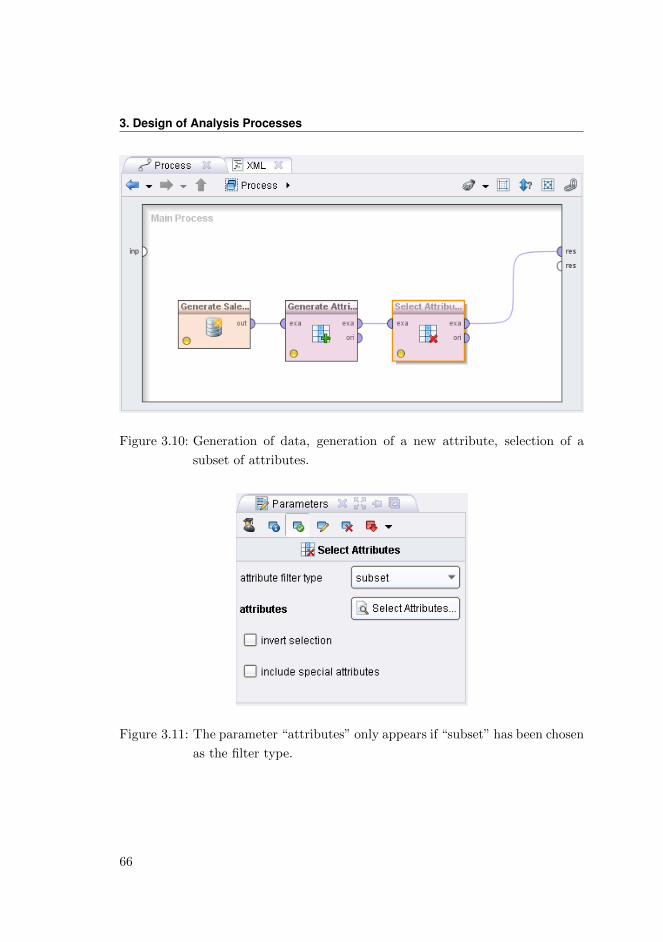
3. Design of Analysis Processes
Figure 3.10: Generation of data, generation of a new attribute, selection of a
subset of attributes.
Figure 3.11: The parameter “attributes” only appears if “subset” has been chosen
as the filter type.
66
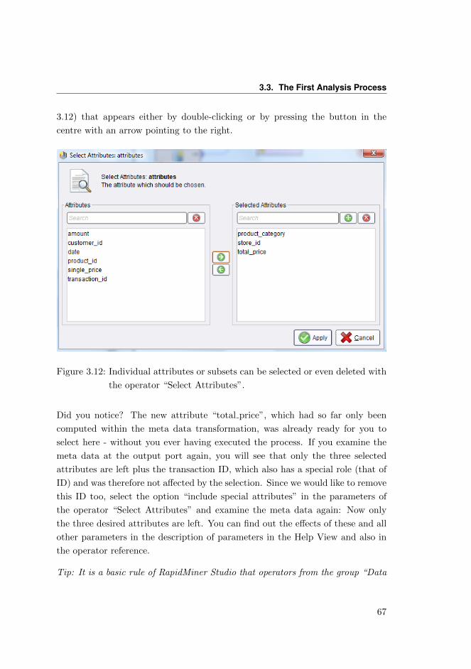
3.3. The First Analysis Process
3.12) that appears either by double-clicking or by pressing the button in the
centre with an arrow pointing to the right.
Figure 3.12: Individual attributes or subsets can be selected or even deleted with
the operator “Select Attributes”.
Did you notice? The new attribute “total price”, which had so far only been
computed within the meta data transformation, was already ready for you to
select here - without you ever having executed the process. If you examine the
meta data at the output port again, you will see that only the three selected
attributes are left plus the transaction ID, which also has a special role (that of
ID) and was therefore not affected by the selection. Since we would like to remove
this ID too, select the option “include special attributes” in the parameters of
the operator “Select Attributes” and examine the meta data again: Now only
the three desired attributes are left. You can find out the effects of these and all
other parameters in the description of parameters in the Help View and also in
the operator reference.
Tip: It is a basic rule of RapidMiner Studio that operators from the group “Data
67
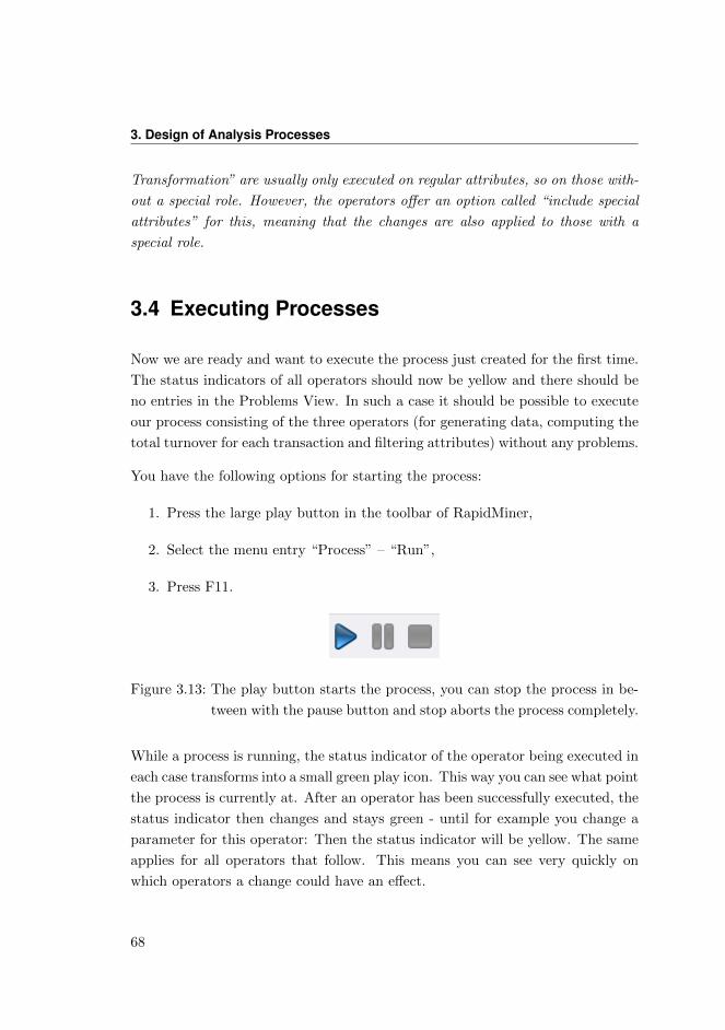
3. Design of Analysis Processes
Transformation” are usually only executed on regular attributes, so on those with-
out a special role. However, the operators offer an option called “include special
attributes” for this, meaning that the changes are also applied to those with a
special role.
3.4 Executing Processes
Now we are ready and want to execute the process just created for the first time.
The status indicators of all operators should now be yellow and there should be
no entries in the Problems View. In such a case it should be possible to execute
our process consisting of the three operators (for generating data, computing the
total turnover for each transaction and filtering attributes) without any problems.
You have the following options for starting the process:
1. Press the large play button in the toolbar of RapidMiner,
2. Select the menu entry “Process” – “Run”,
3. Press F11.
Figure 3.13: The play button starts the process, you can stop the process in be-
tween with the pause button and stop aborts the process completely.
While a process is running, the status indicator of the operator being executed in
each case transforms into a small green play icon. This way you can see what point
the process is currently at. After an operator has been successfully executed, the
status indicator then changes and stays green - until for example you change a
parameter for this operator: Then the status indicator will be yellow. The same
applies for all operators that follow. This means you can see very quickly on
which operators a change could have an effect.
68
3.4. Executing Processes
The process defined above only has a short runtime and so you will hardly have
the opportunity to pause the running process. In principle however you can
briefly stop a running process with the pause symbol e.g. in order to see an
intermediate result. The operator currently being executed is then finished and
the process is then stopped. You can recognise a process that is still running but
currently paused by the fact that the colour of the play icon changes from blue
to green. Press the play button again to continue executing the process further.
If you do not wish to merely pause the process but to abort it completely, then
you can press the stop button. Just like when pausing, the operator currently
being executed is finished and the process fully aborted immediately after. Please
note that you can switch to the Design Perspective immediately after aborting
the process and make changes to processes, even if the execution of the current
operator is being finished in the background. You can even start further processes
and do not need to wait for the first process to be completed.
Note: It was explained above that the operator being executed is always com-
pleted if you abort. This is necessary to ensure a sound execution of operators.
However, completing an operator may need much more time in individual cases
and also require other resources such as storage space. So when you are aborting
very complex operators you can see this taking hours and requiring additional
resources, then your only option is to restart the application.
3.4.1 Looking at Results
After the process was terminated, RapidMiner Studio should have switched to
the Result Perspective (Fig. 3.14). If this was not the case, then you probably
did not connect the output port of the last operator with one of the result ports
of the process on the right-hand side. Check this and also check for other possible
errors, taking the notes in the Problems View into consideration.
Feel free to spend a little time with the results. Since the process above has not
yet performed any modelling but only transformed data, the result only consists
of an example set. You can look at the meta data of this data set and try out the
table plus some of the visualisations in Charts or Advanced Charts. In the next
69
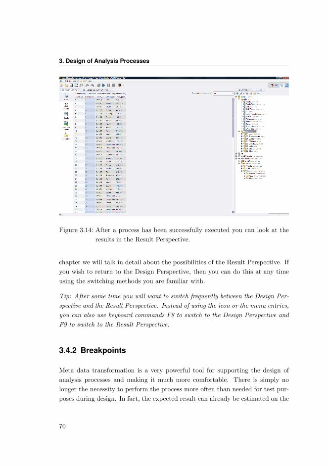
3. Design of Analysis Processes
Figure 3.14: After a process has been successfully executed you can look at the
results in the Result Perspective.
chapter we will talk in detail about the possibilities of the Result Perspective. If
you wish to return to the Design Perspective, then you can do this at any time
using the switching methods you are familiar with.
Tip: After some time you will want to switch frequently between the Design Per-
spective and the Result Perspective. Instead of using the icon or the menu entries,
you can also use keyboard commands F8 to switch to the Design Perspective and
F9 to switch to the Result Perspective.
3.4.2 Breakpoints
Meta data transformation is a very powerful tool for supporting the design of
analysis processes and making it much more comfortable. There is simply no
longer the necessity to perform the process more often than needed for test pur-
poses during design. In fact, the expected result can already be estimated on the
70
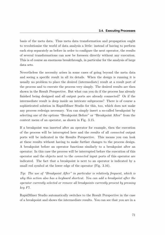
3.4. Executing Processes
basis of the meta data. Thus meta data transformation and propagation ought
to revolutionise the world of data analysis a little: instead of having to perform
each step separately as before in order to configure the next operator, the results
of several transformations can now be foreseen directly without any execution.
This is of course an enormous breakthrough, in particular for the analysis of large
data sets.
Nevertheless the necessity arises in some cases of going beyond the meta data
and seeing a specific result in all its details. When the design is running it is
usually no problem to place the desired (intermediate) result at a result port of
the process and to execute the process very simply. The desired results are then
shown in the Result Perspective. But what can you do if the process has already
finished being designed and all output ports are already connected? Or if the
intermediate result is deep inside an intricate subprocess? There is of course a
sophisticated solution in RapidMiner Studio for this, too, which does not make
any process redesign necessary. You can simply insert a so-called breakpoint by
selecting one of the options “Breakpoint Before” or “Breakpoint After” from the
context menu of an operator, as shown in Fig. 3.15.
If a breakpoint was inserted after an operator for example, then the execution
of the process will be interrupted here and the results of all connected output
ports will be indicated in the Results Perspective. This means you can look
at these results without having to make further changes to the process design.
A breakpoint before an operator functions similarly to a breakpoint after an
operator: In this case the process will be interrupted before the execution of this
operator and the objects next to the connected input ports of this operator are
indicated. The fact that a breakpoint is next to an operator is indicated by a
small red symbol at the lower edge of the operator (Fig. 3.16).
Tip: The use of “Breakpoint After” in particular is relatively frequent, which is
why this action also has a keyboard shortcut. You can add a breakpoint after the
operator currently selected or remove all breakpoints currently present by pressing
key F7.
RapidMiner Studio automatically switches to the Result Perspective in the case
of a breakpoint and shows the intermediate results. You can see that you are in a
71
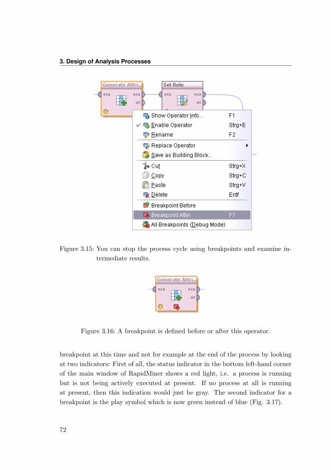
3. Design of Analysis Processes
Figure 3.15: You can stop the process cycle using breakpoints and examine in-
termediate results.
Figure 3.16: A breakpoint is defined before or after this operator.
breakpoint at this time and not for example at the end of the process by looking
at two indicators: First of all, the status indicator in the bottom left-hand corner
of the main window of RapidMiner shows a red light, i.e. a process is running
but is not being actively executed at present. If no process at all is running
at present, then this indication would just be gray. The second indicator for a
breakpoint is the play symbol which is now green instead of blue (Fig. 3.17).
72
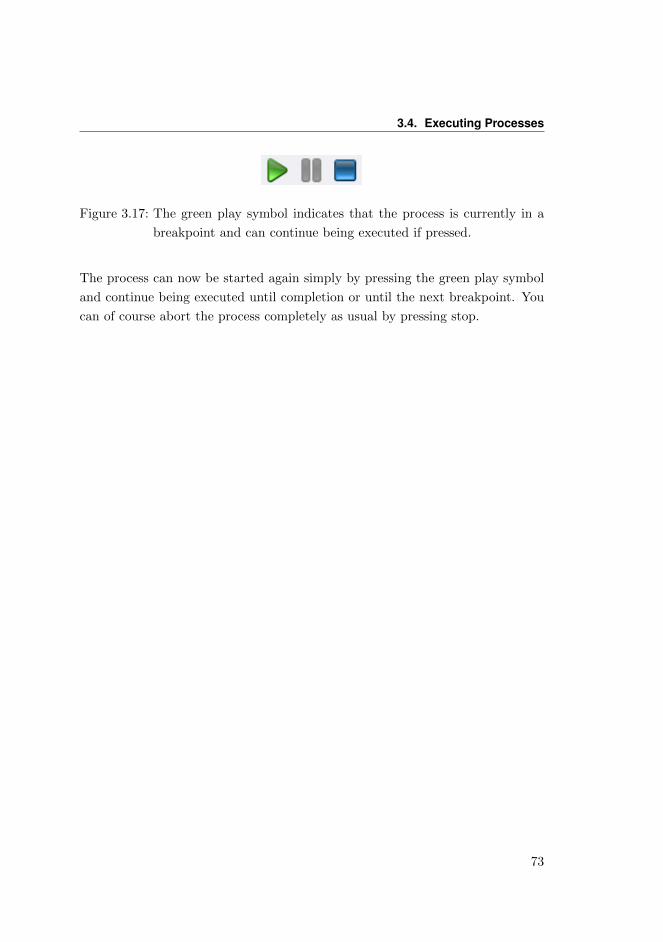
3.4. Executing Processes
Figure 3.17: The green play symbol indicates that the process is currently in a
breakpoint and can continue being executed if pressed.
The process can now be started again simply by pressing the green play symbol
and continue being executed until completion or until the next breakpoint. You
can of course abort the process completely as usual by pressing stop.
73

4 Data andResult Visualization
In the previous sections we have seen how the graphical user interface of Rapid-
Miner Studio is built up and how you can define and execute analysis processes
with it. At the end of such a process the results of the process can then be
indicated in the Results Perspective. Switch now to this Results Perspective by
clicking once in the toolbar. This will be dealt with in detail within this chap-
ter. Depending on whether you have already produced representable results, you
should now see, in the original settings at least, roughly the screen shown in 4.1.
Otherwise, you can recreate this preset perspective under “View” – “Restore De-
fault Perspective” as always. The Result Perspective is the second central work-
ing environment of RapidMiner Studio alongside the Design Perspective already
discussed. We have already discussed the Repositories View on the right. In this
chapter we will therefore focus on the remaining component of the perspective.
4.1 Result Visualization
We have already seen that objects which are placed at the result ports at the
right-hand side of a process are automatically displayed in the Results Perspective
after the process is completed. The large area on the top left-hand side is used
here, where the Results Overview is also already displayed, which we will discuss
at the end of this chapter.
75

4. Data and Result Visualization
Figure 4.1: Result Perspective of RapidMiner.
Each currently opened and indicated result is displayed as an additional tab in
this area like in Figure 4.2. Strictly speaking, each result is also a view, which
you can move to anywhere you wish as usual. In this way it is possible to look
at several results at the same time.
You can of course also close individual views, i.e. tabs, by clicking once on the
cross on the tab. The other functionalities of views, such as maximisation are also
completely available to you here. RapidMiner Studio will close the old results
before the new results are displayed.
4.1.1 Sources for Displaying Results
There are several sources from which you can have results displayed. We will
present all ways to you in the following:
76
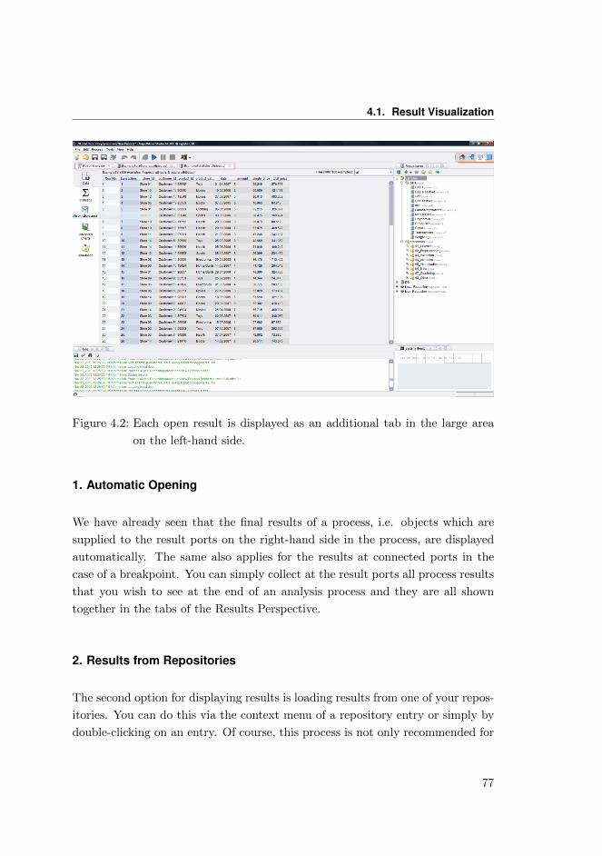
4.1. Result Visualization
Figure 4.2: Each open result is displayed as an additional tab in the large area
on the left-hand side.
1. Automatic Opening
We have already seen that the final results of a process, i.e. objects which are
supplied to the result ports on the right-hand side in the process, are displayed
automatically. The same also applies for the results at connected ports in the
case of a breakpoint. You can simply collect at the result ports all process results
that you wish to see at the end of an analysis process and they are all shown
together in the tabs of the Results Perspective.
2. Results from Repositories
The second option for displaying results is loading results from one of your repos-
itories. You can do this via the context menu of a repository entry or simply by
double-clicking on an entry. Of course, this process is not only recommended for
77
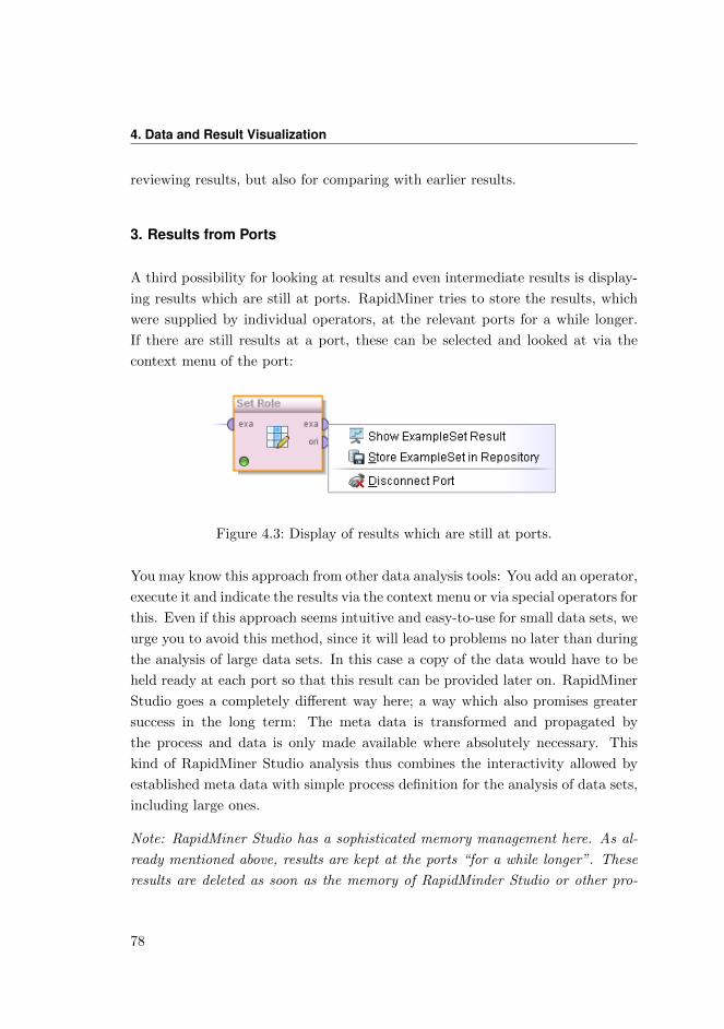
4. Data and Result Visualization
reviewing results, but also for comparing with earlier results.
3. Results from Ports
A third possibility for looking at results and even intermediate results is display-
ing results which are still at ports. RapidMiner tries to store the results, which
were supplied by individual operators, at the relevant ports for a while longer.
If there are still results at a port, these can be selected and looked at via the
context menu of the port:
Figure 4.3: Display of results which are still at ports.
You may know this approach from other data analysis tools: You add an operator,
execute it and indicate the results via the context menu or via special operators for
this. Even if this approach seems intuitive and easy-to-use for small data sets, we
urge you to avoid this method, since it will lead to problems no later than during
the analysis of large data sets. In this case a copy of the data would have to be
held ready at each port so that this result can be provided later on. RapidMiner
Studio goes a completely different way here; a way which also promises greater
success in the long term: The meta data is transformed and propagated by
the process and data is only made available where absolutely necessary. This
kind of RapidMiner Studio analysis thus combines the interactivity allowed by
established meta data with simple process definition for the analysis of data sets,
including large ones.
Note: RapidMiner Studio has a sophisticated memory management here. As al-
ready mentioned above, results are kept at the ports “for a while longer”. These
results are deleted as soon as the memory of RapidMinder Studio or other pro-
78
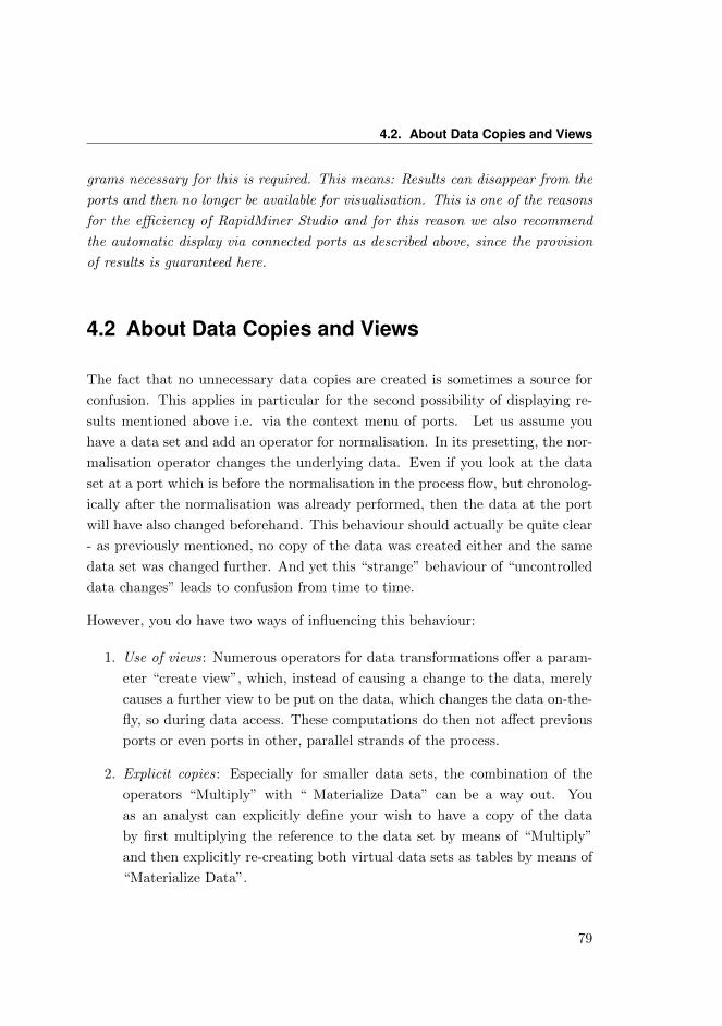
4.2. About Data Copies and Views
grams necessary for this is required. This means: Results can disappear from the
ports and then no longer be available for visualisation. This is one of the reasons
for the efficiency of RapidMiner Studio and for this reason we also recommend
the automatic display via connected ports as described above, since the provision
of results is guaranteed here.
4.2 About Data Copies and Views
The fact that no unnecessary data copies are created is sometimes a source for
confusion. This applies in particular for the second possibility of displaying re-
sults mentioned above i.e. via the context menu of ports. Let us assume you
have a data set and add an operator for normalisation. In its presetting, the nor-
malisation operator changes the underlying data. Even if you look at the data
set at a port which is before the normalisation in the process flow, but chronolog-
ically after the normalisation was already performed, then the data at the port
will have also changed beforehand. This behaviour should actually be quite clear
- as previously mentioned, no copy of the data was created either and the same
data set was changed further. And yet this “strange” behaviour of “uncontrolled
data changes” leads to confusion from time to time.
However, you do have two ways of influencing this behaviour:
1. Use of views: Numerous operators for data transformations offer a param-
eter “create view”, which, instead of causing a change to the data, merely
causes a further view to be put on the data, which changes the data on-the-
fly, so during data access. These computations do then not affect previous
ports or even ports in other, parallel strands of the process.
2. Explicit copies: Especially for smaller data sets, the combination of the
operators “Multiply” with “ Materialize Data” can be a way out. You
as an analyst can explicitly define your wish to have a copy of the data
by first multiplying the reference to the data set by means of “Multiply”
and then explicitly re-creating both virtual data sets as tables by means of
“Materialize Data”.
79
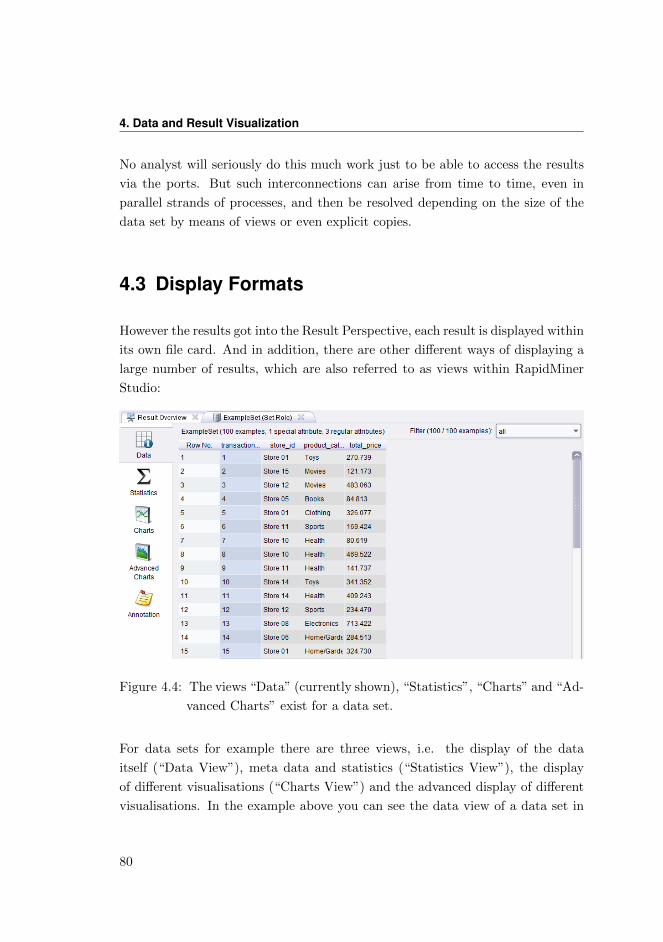
4. Data and Result Visualization
No analyst will seriously do this much work just to be able to access the results
via the ports. But such interconnections can arise from time to time, even in
parallel strands of processes, and then be resolved depending on the size of the
data set by means of views or even explicit copies.
4.3 Display Formats
However the results got into the Result Perspective, each result is displayed within
its own file card. And in addition, there are other different ways of displaying a
large number of results, which are also referred to as views within RapidMiner
Studio:
Figure 4.4: The views “Data” (currently shown), “Statistics”, “Charts” and “Ad-
vanced Charts” exist for a data set.
For data sets for example there are three views, i.e. the display of the data
itself (“Data View”), meta data and statistics (“Statistics View”), the display
of different visualisations (“Charts View”) and the advanced display of different
visualisations. In the example above you can see the data view of a data set in
80
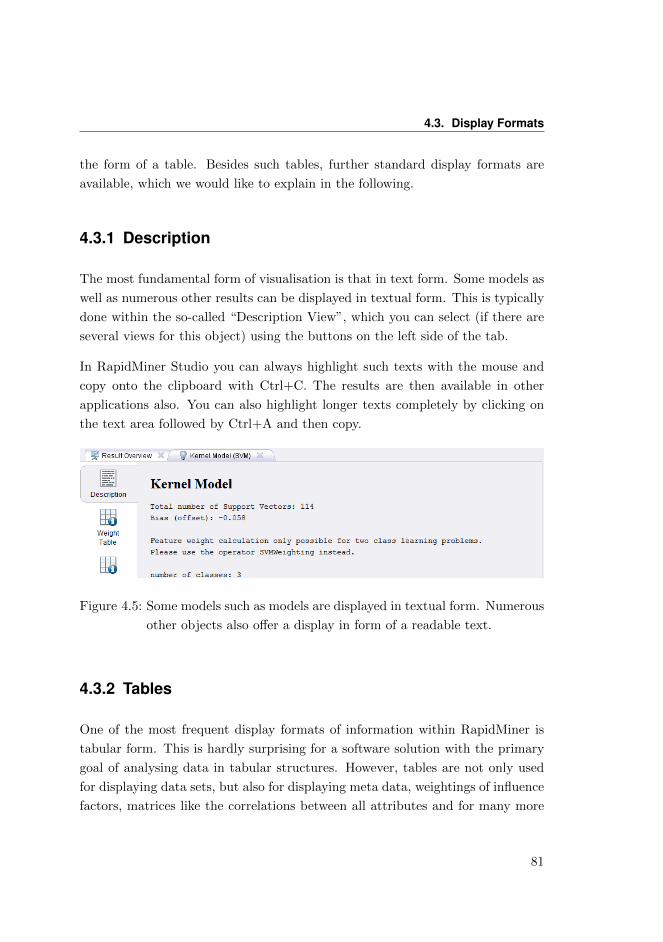
4.3. Display Formats
the form of a table. Besides such tables, further standard display formats are
available, which we would like to explain in the following.
4.3.1 Description
The most fundamental form of visualisation is that in text form. Some models as
well as numerous other results can be displayed in textual form. This is typically
done within the so-called “Description View”, which you can select (if there are
several views for this object) using the buttons on the left side of the tab.
In RapidMiner Studio you can always highlight such texts with the mouse and
copy onto the clipboard with Ctrl+C. The results are then available in other
applications also. You can also highlight longer texts completely by clicking on
the text area followed by Ctrl+A and then copy.
Figure 4.5: Some models such as models are displayed in textual form. Numerous
other objects also offer a display in form of a readable text.
4.3.2 Tables
One of the most frequent display formats of information within RapidMiner is
tabular form. This is hardly surprising for a software solution with the primary
goal of analysing data in tabular structures. However, tables are not only used
for displaying data sets, but also for displaying meta data, weightings of influence
factors, matrices like the correlations between all attributes and for many more
81
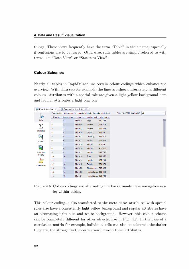
4. Data and Result Visualization
things. These views frequently have the term “Table” in their name, especially
if confusions are to be feared. Otherwise, such tables are simply referred to with
terms like “Data View” or “Statistics View”.
Colour Schemes
Nearly all tables in RapidMiner use certain colour codings which enhance the
overview. With data sets for example, the lines are shown alternately in different
colours. Attributes with a special role are given a light yellow background here
and regular attributes a light blue one:
Figure 4.6: Colour codings and alternating line backgrounds make navigation eas-
ier within tables.
This colour coding is also transferred to the meta data: attributes with special
roles also have a consistently light yellow background and regular attributes have
an alternating light blue and white background. However, this colour scheme
can be completely different for other objects, like in Fig. 4.7. In the case of a
correlation matrix for example, individual cells can also be coloured: the darker
they are, the stronger is the correlation between these attributes.
82
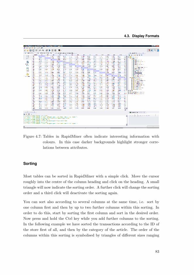
4.3. Display Formats
Figure 4.7: Tables in RapidMiner often indicate interesting information with
colours. In this case darker backgrounds highlight stronger corre-
lations between attributes.
Sorting
Most tables can be sorted in RapidMiner with a simple click. Move the cursor
roughly into the centre of the column heading and click on the heading. A small
triangle will now indicate the sorting order. A further click will change the sorting
order and a third click will deactivate the sorting again.
You can sort also according to several columns at the same time, i.e. sort by
one column first and then by up to two further columns within this sorting. In
order to do this, start by sorting the first column and sort in the desired order.
Now press and hold the Ctrl key while you add further columns to the sorting.
In the following example we have sorted the transactions according to the ID of
the store first of all, and then by the category of the article. The order of the
columns within this sorting is symbolised by triangles of different sizes ranging
83

4. Data and Result Visualization
from large to small (Fig. 4.8).
Figure 4.8: Sorting was first performed in this table in ascending order according
to the attribute “store id” and then according to product category
within the store ID blocks, also in ascending order.
Note: Sorting can be time-consuming. It is therefore deactivated for large tables,
so that no sorting is started inadvertently and the program cannot be used in
this time. You can set the threshold value at which sorting is deactivated in the
settings under “Tools” – “Preferences”.
Moving Columns
You can change the order of columns in most tables by clicking on the column
heading and dragging the column to a new position while holding down the mouse
button. This can be practical if you wish to compare the contents of two columns
with one another in large tables.
Adjusting Column Widths
You can adjust the width of columns by holding the cursor over the area between
two columns and changing the width of the column to the left of the separation
84
4.3. Display Formats
area while holding down the mouse button. Alternatively, you can also double-
click on this gap, which causes the width of the column to the left of the gap
to be automatically adjusted to the necessary minimum size. Last but not least,
you can also hold the Ctrl key down when you double-click on a gap, causing the
size of all columns to be adapted automatically.
Tip: You should note this combination (CTRL + double click on a gap in the
column heading area) so that you can quickly adjust column widths.
Actions in the Context Menu
In most tables you can open a context menu with further actions by right-clicking
on a table cell. The details of these actions are:
1. Select Row: Selecting a line,
2. Select Column: Selecting a column
3. Fit Column Width: Adjusting the width of the selected column
4. Fit all Column Widths: Adjusting all column widths
5. Equal Column Widths: Using same standard width for all columns
6. Sort by Column (Ascending): Sorting by this column in ascending order
7. Sort by Column (Descending): Sorting by this column in descending order
8. Add to Sorting Columns (Ascending): Adding to the sorting columns (as-
cending)
9. Add to Sorting Columns (Descending): Adding to the sorting columns (de-
scending)
10. Sort Columns by Names: Reordering columns by sorting the column head-
ings in alphabetical order
11. Restore Column Order: Restoring the original column order.
85
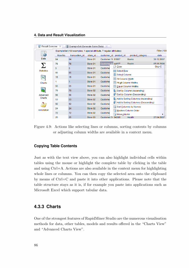
4. Data and Result Visualization
Figure 4.9: Actions like selecting lines or columns, sorting contents by columns
or adjusting column widths are available in a context menu.
Copying Table Contents
Just as with the text view above, you can also highlight individual cells within
tables using the mouse or highlight the complete table by clicking in the table
and using Ctrl+A. Actions are also available in the context menu for highlighting
whole lines or columns. You can then copy the selected area onto the clipboard
by means of Ctrl+C and paste it into other applications. Please note that the
table structure stays as it is, if for example you paste into applications such as
Microsoft Excel which support tabular data.
4.3.3 Charts
One of the strongest features of RapidMiner Studio are the numerous visualisation
methods for data, other tables, models and results offered in the “Charts View”
and “Advanced Charts View”.
86
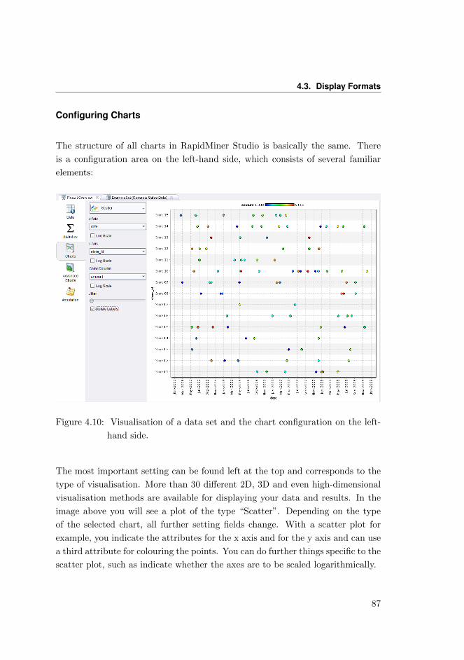
4.3. Display Formats
Configuring Charts
The structure of all charts in RapidMiner Studio is basically the same. There
is a configuration area on the left-hand side, which consists of several familiar
elements:
Figure 4.10: Visualisation of a data set and the chart configuration on the left-
hand side.
The most important setting can be found left at the top and corresponds to the
type of visualisation. More than 30 different 2D, 3D and even high-dimensional
visualisation methods are available for displaying your data and results. In the
image above you will see a plot of the type “Scatter”. Depending on the type
of the selected chart, all further setting fields change. With a scatter plot for
example, you indicate the attributes for the x axis and for the y axis and can use
a third attribute for colouring the points. You can do further things specific to the
scatter plot, such as indicate whether the axes are to be scaled logarithmically.
87
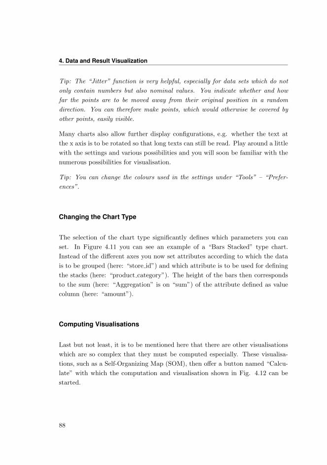
4. Data and Result Visualization
Tip: The “Jitter” function is very helpful, especially for data sets which do not
only contain numbers but also nominal values. You indicate whether and how
far the points are to be moved away from their original position in a random
direction. You can therefore make points, which would otherwise be covered by
other points, easily visible.
Many charts also allow further display configurations, e.g. whether the text at
the x axis is to be rotated so that long texts can still be read. Play around a little
with the settings and various possibilities and you will soon be familiar with the
numerous possibilities for visualisation.
Tip: You can change the colours used in the settings under “Tools” – “Prefer-
ences”.
Changing the Chart Type
The selection of the chart type significantly defines which parameters you can
set. In Figure 4.11 you can see an example of a “Bars Stacked” type chart.
Instead of the different axes you now set attributes according to which the data
is to be grouped (here: “store id”) and which attribute is to be used for defining
the stacks (here: “product category”). The height of the bars then corresponds
to the sum (here: “Aggregation” is on “sum”) of the attribute defined as value
column (here: “amount”).
Computing Visualisations
Last but not least, it is to be mentioned here that there are other visualisations
which are so complex that they must be computed especially. These visualisa-
tions, such as a Self-Organizing Map (SOM), then offer a button named “Calcu-
late” with which the computation and visualisation shown in Fig. 4.12 can be
started.
88
4.3. Display Formats
Figure 4.11: Change of the chart configuration depending on the chart type.
4.3.4 Graphs
Graphs are a further display format which are found relatively frequently in
RapidMiner. Graphs basically mean all visualisations which show nodes and
their relationships. These can be nodes within a hierarchical clustering or the
nodes of a decision tree as in Figure 4.13.
Graphs like that of the decision tree are mostly referred to as a “Graph View”
and are available under this name.
Zooming
Using the mouse wheel, if there is one, you can zoom in on and out from the
graphs. Alternatively, you also have two buttons on the top left-hand side of the
configuration area with which you can increase and reduce the zoom level of your
graph.
89
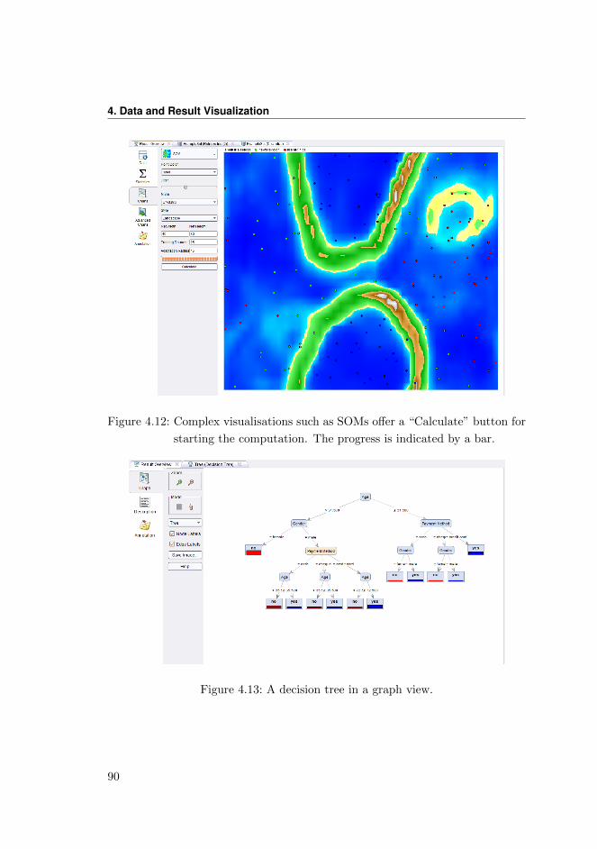
4. Data and Result Visualization
Figure 4.12: Complex visualisations such as SOMs offer a “Calculate” button for
starting the computation. The progress is indicated by a bar.
Figure 4.13: A decision tree in a graph view.
90
4.3. Display Formats
Mode
Two fundamental navigation methods are available in the graph, which are also
called modes:
1. Moving : The mode for moving the graph is selected by pressing the left-
hand button in the mode box. In this case you can move the section of the
graph while holding down the left mouse button in order to view different
areas of the graph in detail.
2. Selecting : The mode for selecting individual nodes is selected by pressing
the right-hand button in the mode box. Now you can select individual
nodes by clicking on them or, while holding down the mouse button, define
a selection box in a free area for several nodes at the same time. By holding
down the Shift key you can add individual nodes to the selection or exclude
them from the selection. Nodes that are currently selected can be moved
while holding down the mouse button.
You will find further notes on handling graphs in these two modes in the help
dialog, which is shown if you click on the button “Help” in the configuration area
of the graph.
Further Settings
You can set whether the captions for nodes and edges are to be shown or not.
The most important setting, not necessarily for trees but for other graphs, is
the choice of a suitable layout, which can be made in the selection box directly
underneath the mode box. The different algorithms have different strengths and
weaknesses and you usually have to try and see which display gives the best result
for the graph at hand.
91
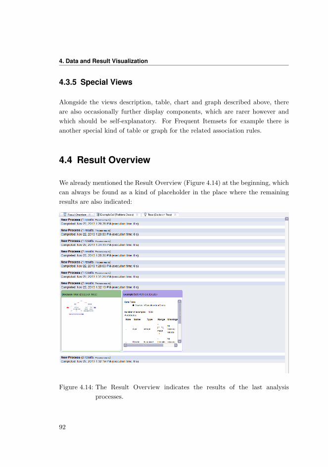
4. Data and Result Visualization
4.3.5 Special Views
Alongside the views description, table, chart and graph described above, there
are also occasionally further display components, which are rarer however and
which should be self-explanatory. For Frequent Itemsets for example there is
another special kind of table or graph for the related association rules.
4.4 Result Overview
We already mentioned the Result Overview (Figure 4.14) at the beginning, which
can always be found as a kind of placeholder in the place where the remaining
results are also indicated:
Figure 4.14: The Result Overview indicates the results of the last analysis
processes.
92
4.4. Result Overview
The Result Overview serves as a compact overview of all process executions of
the current RapidMiner session. Each two-line entry consists of the name of the
process, the number of the results as well as information on when the process
was completed and how long it ran for. Each block displaying results of the same
process have an alternate colouring.
You can see a detailed view of the results by clicking on an entry. In the case
above the result consists of an example set and a decision tree. A further click
on the entry will close it again. You can of course also open several entries at the
same time and compare the results comfortably by doing so.
Two actions are available for each entry on the top right:
• To restore the process belonging to an entry in this form and
• To delete the entry from the Result Overview.
In addition, you have the option to delete the complete overview in the context
menus of the Overview and of the individual entries.
93

5 ManagingData: The Repository
Tables, databases, collections of texts, log files, websites, measured values – this
and the like is at the beginning of every data mining process. Data is prepared,
converted, merged, and at the end you will receive new or differently represented
data, models or reports. In this chapter you will find out how to handle all these
objects with RapidMiner Studio.
5.1 The RapidMiner Studio Repository
As soon as your collection of processes and associated files exceeds a certain size,
you will see it is wise to organise those in a consistent and structured manner.
One possibility is the organisation of projects on file level. Files are grouped into
projects and a directory is created in each case for output data, intermediate
results, reports, etc.
While creating organised project structures is sensible, using the normal file sys-
tem is recommended only in the rarest cases and is hardly sufficient for the needs
of a data mining solution. Different reasons such as confidentiality or limited
storage space can make creating files on the local computer impossible. If a pro-
cess created on the local computer is to be executed on a remote server, this
requires manual interventions like copying the process and adapting paths. The
collaborative creation of processes, manipulation of data and evaluation of results
95
5. Repository
requires an external rights and version administration. Files stored in different
formats require the correct setting of parameters such as separators and coding
for each new loading. Intermediate results and process variants soon grow to a
considerable number, meaning that one can lose track easily. Loading and look-
ing at data in order to regain an overview requires a loading process that may
be lengthy or even the running of an external application. Annotations of files
which can make this easier are not supported by normal file systems.
RapidMiner’s answer to all these problems is the repository, which takes up all
data and processes. Although data can also be introduced into processes from
outside the repository, which is necessary for the execution of ETL processes for
example, using the repository offers a number of advantages which you will not
want to miss:
• Data, processes, results and reports are stored in locations indicated relative
to one another in a mechanism that is transparent for the user.
• Opening or loading the files requires no further settings. Data can be
opened, looked at or incorporated into the process with a single click. You
will get an overview of the stored data, its characteristics and remarks made
by yourself at any time without having to open the file separately.
• All input and output data plus intermediate results are annotated with
meta information. This ensures the consistency and integrity of your data
and makes validating processes possible at the time of development as well
as the provision of context-sensitive assistants.
The repository can either be on a local or shared file system or be made available
by the external RapidMiner Server. The following picture shows the repository
view, which displays the content of the repository. RapidMiner Studio provides a
set of example processes and example data which you will find in the repository
initially created. Some of these can be seen in Figure 5.1.
96
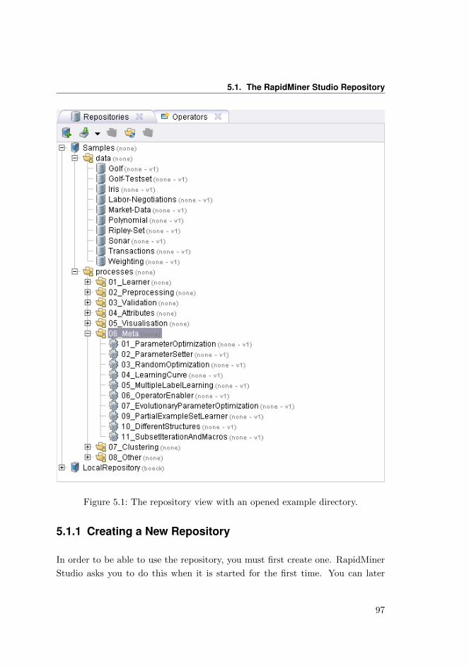
5.1. The RapidMiner Studio Repository
Figure 5.1: The repository view with an opened example directory.
5.1.1 Creating a New Repository
In order to be able to use the repository, you must first create one. RapidMiner
Studio asks you to do this when it is started for the first time. You can later
97
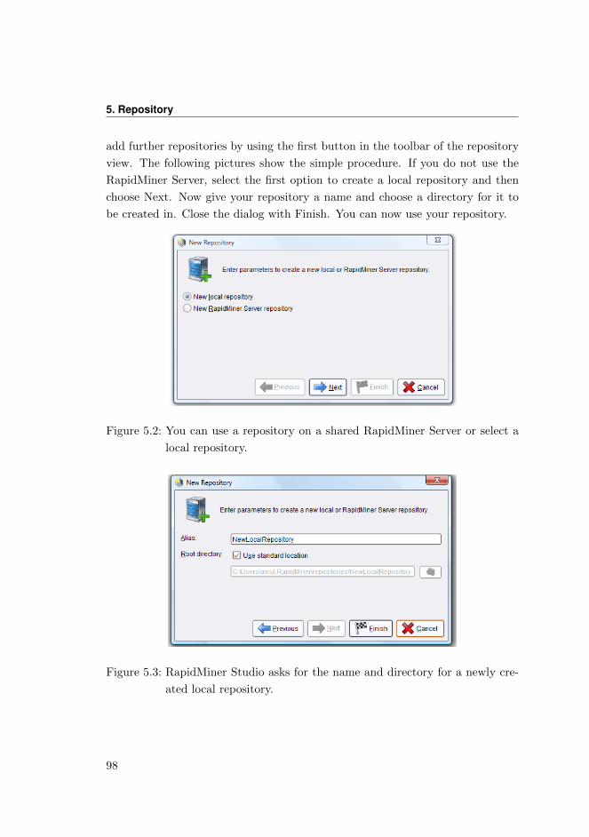
5. Repository
add further repositories by using the first button in the toolbar of the repository
view. The following pictures show the simple procedure. If you do not use the
RapidMiner Server, select the first option to create a local repository and then
choose Next. Now give your repository a name and choose a directory for it to
be created in. Close the dialog with Finish. You can now use your repository.
Figure 5.2: You can use a repository on a shared RapidMiner Server or select a
local repository.
Figure 5.3: RapidMiner Studio asks for the name and directory for a newly cre-
ated local repository.
98
5.2. Using the Repository
5.2 Using the Repository
It makes sense to use a uniform directory structure for projects, for example a
project folder with the name of the project and a folder each for processes, input
data and results. All examples in this manual follow this structure. You can
create directories using the context menu in the repository view or using the
button in the toolbar at the top of this view.
5.2.1 Processes and Relative Repository Descriptions
Before discussing in the following sections how you can store data and processes in
the repository and access these again, we would like to first give some fundamental
tips on referencing these objects within the repository. You can store processes
in the repository by selecting the entry “Store Process” in the context menu
or by selecting the appropriate entry in the “File” menu. In the latter case,
the repository browser opens, where you can indicate the location for storing
the process. After a process has been stored in the repository, all references to
repository entries set as parameters of operators are resolved in relation to the
location of the process. What does that mean? Entries in the repository are
designated as follows:
//RepositoryName/Folder/Subfolder/File
The two slashes at the beginning indicate that the name of a repository will
follow first. Then further folder names and finally a file name. We call such
details absolute. In the following description
/Folder/Subfolder/File
the repository designation is missing at the front. This description is therefore
repository-relative. It refers to the file described in the same repository, where
the process in which this description is used is located. The slash at the front
indicates an absolute path description. If this is also missing, the description
relative is resolved:
99
5. Repository
../RelativeFolder/File
designates for example a file in the folder “RelativeFolder” which we reach by
moving up (“..”) a directory from the file containing the current process and
looking for the folder “RelativeFolder” there. So if the process is located for
example in the file
//MyRepository/ProjectA/Processes/ProcessB,
this description leads to
//MyRepository/ProjectA/RelativeFolder/File.
Note: The descriptions above probably sound more complicated than they really
are in practice. As long as, before anything else, you define a location within the
repository for each new process and then simply use the repository browser for all
operator parameters requiring an entry in the repository, RapidMiner Studio will
ensure, fully automatically, that relative data is always used as far as possible.
This makes repository restructuring and making copies for other users easier in
particular, which would be difficult with absolute descriptions.
5.2.2 Importing Data and Objects into the Repository
There are numerous ways to import data and other objects such as models into
the repository. We will now describe the most important ones.
Importing Example Sets with Wizards
If you have data in a certain format and wish to use it in a RapidMiner Studio
process, so-called wizards are available to you for many file formats and databases.
A wizard is a dialog which guides you step by step through the loading process.
With all wizards you can assign certain meta data such as attribute types, ranges
of values and roles for the individual columns. In the upper area of the repository
you will find an icon which starts the appropriate wizard for the selected file type.
You will find the same action in the “File” menu of RapidMiner Studio. Finally,
100
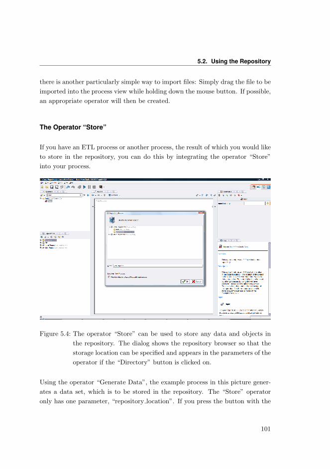
5.2. Using the Repository
there is another particularly simple way to import files: Simply drag the file to be
imported into the process view while holding down the mouse button. If possible,
an appropriate operator will then be created.
The Operator “Store”
If you have an ETL process or another process, the result of which you would like
to store in the repository, you can do this by integrating the operator “Store”
into your process.
Figure 5.4: The operator “Store” can be used to store any data and objects in
the repository. The dialog shows the repository browser so that the
storage location can be specified and appears in the parameters of the
operator if the “Directory” button is clicked on.
Using the operator “Generate Data”, the example process in this picture gener-
ates a data set, which is to be stored in the repository. The “Store” operator
only has one parameter, “repository location”. If you press the button with the
101
5. Repository
folder next to this parameter, you will get a dialog in which you can first assign
a folder in the repository and then a name for the data set (Figure 5.4). If you
execute the process, you will see that a new entry will appear in the repository
containing the generated data set. The store operator is therefore particularly
useful for data integration and transformation processes which are to be per-
formed automatically or regularly, for example within the process scheduler of
the RapidMiner Server. Using the wizard as described above is definitely the
more frequently used way to ensure a one-off and fairly interactive integration of
data.
Note: You can not only connect data sets with the store operator, but also models
and all other RapidMiner Studio objects. You can therefore also store any results
in your repository.
Importing other formats with operators
The repository stores data sets in a format which contains all data and meta data
needed by RapidMiner Studio. Your data will probably be in another format at
the beginning: CSV, Excel, SQL databases, etc. As described above, you can
transfer these files into your repository. However, RapidMiner Studio can also
import numerous other formats within processes. You will find operators for this
in the group “Import”. However, caution is required when using these operators:
The availability of meta data is not guaranteed for these operators, which can
lead for example to processes that assume the existence of certain attribute values
only noticing any errors in the runtime of the process. Nevertheless, using these
file formats is sometimes not avoidable, e.g. for the regular execution of ETL
processes. The goal of these processes should be however to transfer the data
into the repository with a subsequent store operator so that it can be used by
the actual analysis processes that follow.
The operators of the “Import” group have numerous parameters tailored to the
respective format. Please see the respective operator documentation for their
description.
102
5.2. Using the Repository
Storing Objects from the Result or Process View
After you have executed a process, the Results Perspective with the tab of the
same name is presented to you in the basic setting. On the right-hand side of its
toolbar there is a button with which you can store the result currently selected
in the repository. A dialog will also appear here allowing you to select a folder
and a name.
If your process contains intermediate results which are not (or no longer) indicated
in the Results Perspective, you can also store these from the Process View. In
order to do this, click on a port where data is present using the right-hand mouse
button. This is the case at the output ports of all operators that have already
been executed. You will recognise this from the darker colour and an appropriate
entry in the context help. You select the menu entry “Store in Repository” here
to store the object. Please bear in mind however that the data at the ports
may be released again after some time in order to save memory and is therefore
not guaranteed to stay at the ports for any amount of time. Please also see the
explanations in the previous chapter.
5.2.3 Access to and Administration of the Repository
Once you have imported your data into the repository you can use it in your
processes with the retrieve operator. You can drag the operator from the Oper-
ators View into the process as usual and define the parameter for the repository
entry there. But it gets easier still: Simply drag an entry in the repository (e.g.
a data set) onto the Process View using the mouse. A configured operator with
a reference to this entry will now be inserted automatically here. If the entry is
an object, a new operator of the “Retrieve” type will be created and configured
accordingly. If the repository entry is a process however, then a new operator of
the “Execute Process” type will be created and its parameter will automatically
refer to the selected process from the repository.
You will find further ways of accessing the repository by right-clicking once on
entries in the repository. You will be familiar with these possibilities from the file
103
5. Repository
management of your computer. These actions are also available via the toolbar
of the repository view and are largely self-explanatory:
Store Process here Stores the current process to the location indicated
Rename Renames the entry or the directory
Create Folder Creates a new folder here
Delete Deletes the selected repository entry or directory
Copy Copies the selected entry so it can be pasted in other places later on
Paste Pastes a previously copied entry to this place
Copy Location to Clipboard Copies a clear identifier for this entry onto the clip-
board, meaning you can use this as a parameter for operators, in web in-
terfaces or the like
Open Process If you have selected a process, the current process will be closed
and the selected one loaded
Refresh If the repository is located on a shared file system or if you use Rapid-
Miner Server, meaning data can be changed at the same time by other
users, you can refresh the view of the repository with this
5.2.4 The Process Context
We have already used the output ports of the process on the right-hand side
of the Process View previously e.g. in order to make the results of the process
visible in the Result Perspective. In addition to the output ports of the process
there are also input ports, which you will find on the left-hand side of the Process
View. We have never connected these before. This is not even worthwhile in the
basic setting, at least not for the sources, because the process itself then has no
input. Connecting the inner sinks does have an effect however: All objects which
arrive at a sink at the end of the process are presented in the Result Perspective
as the result of the process.
104
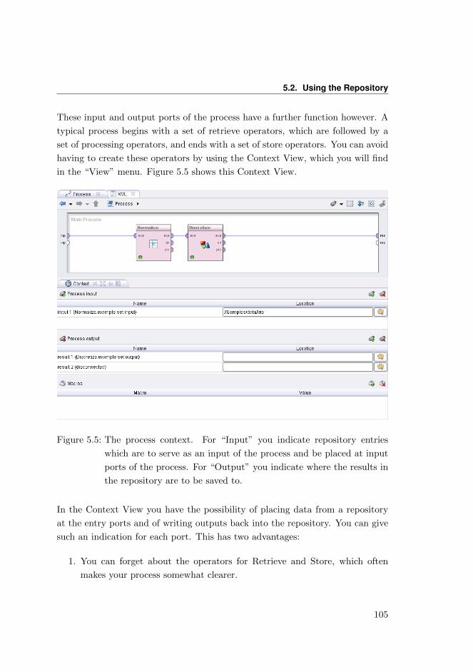
5.2. Using the Repository
These input and output ports of the process have a further function however. A
typical process begins with a set of retrieve operators, which are followed by a
set of processing operators, and ends with a set of store operators. You can avoid
having to create these operators by using the Context View, which you will find
in the “View” menu. Figure 5.5 shows this Context View.
Figure 5.5: The process context. For “Input” you indicate repository entries
which are to serve as an input of the process and be placed at input
ports of the process. For “Output” you indicate where the results in
the repository are to be saved to.
In the Context View you have the possibility of placing data from a repository
at the entry ports and of writing outputs back into the repository. You can give
such an indication for each port. This has two advantages:
1. You can forget about the operators for Retrieve and Store, which often
makes your process somewhat clearer.
105
5. Repository
2. Using the context is also practical for testing processes which are to be
integrated by means of the operator “Execute Process”: The data at this
operator will overwrite the values defined in the process context.
5.3 Data and Meta Data
Apart from the actual data, RapidMiner Studio also stores other information in
the repository: Data about the data, so-called meta data. Such meta data is
available for each type of object, and it can be particularly useful for models and
data sets. The meta information stored for data sets includes for example:
• The number of examples
• The number of attributes
• The types, names and roles of the attributes
• The ranges of values of the attributes or some fundamental statistics
• plus the number of missing values per attribute.
This information can be seen in the repository without loading the data set
beforehand, which can take some time depending on size. Simply move the
cursor over a repository entry and stay on the entry for a few seconds: The
meta data will be presented to you in the form of a so-called tooltip. Unlike
in other programs, this help information is much more powerful than normal:
By pressing key F3 you can turn such a tooltip into a proper dialog, which you
can move around and change in size as you wish. In addition, these RapidMiner
Studio tooltips are also able to include elements other than textual information
with the meta data, such as tables for example.
Please note that the meta information does not necessarily have to be available
immediately. You may have to first initiate the loading of the meta data by click-
ing once on a link within the tooltip. Doing this means that, should the tooltips
of the repository entries be inadvertently looked at, the possibly quite large meta
106
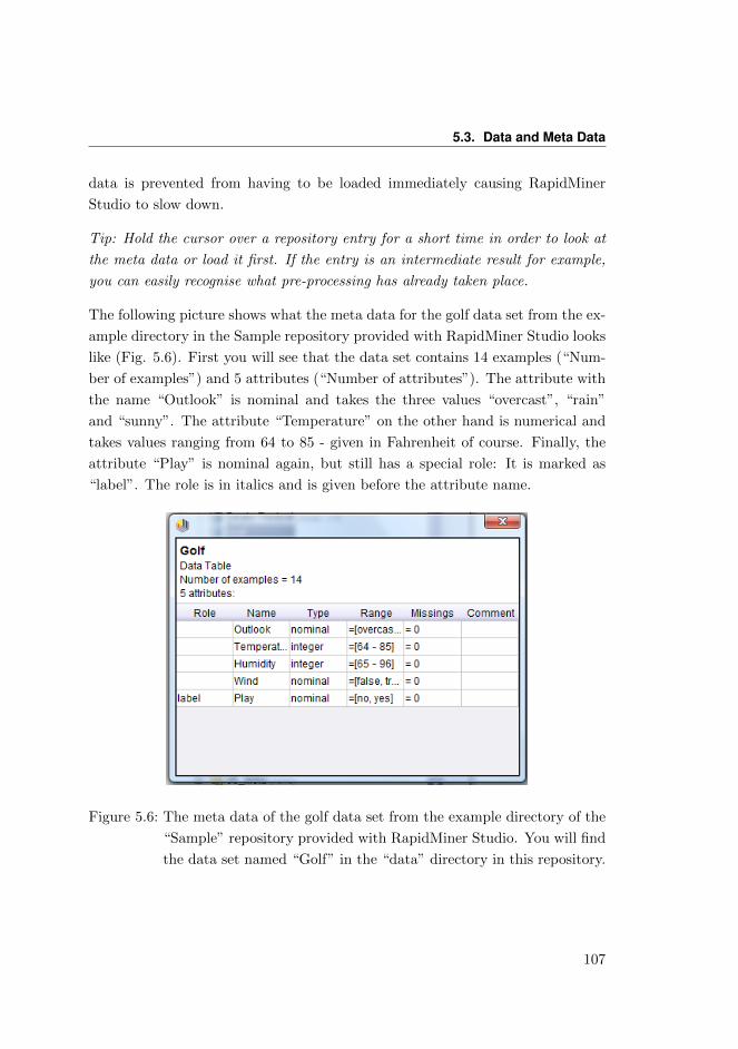
5.3. Data and Meta Data
data is prevented from having to be loaded immediately causing RapidMiner
Studio to slow down.
Tip: Hold the cursor over a repository entry for a short time in order to look at
the meta data or load it first. If the entry is an intermediate result for example,
you can easily recognise what pre-processing has already taken place.
The following picture shows what the meta data for the golf data set from the ex-
ample directory in the Sample repository provided with RapidMiner Studio looks
like (Fig. 5.6). First you will see that the data set contains 14 examples (“Num-
ber of examples”) and 5 attributes (“Number of attributes”). The attribute with
the name “Outlook” is nominal and takes the three values “overcast”, “rain”
and “sunny”. The attribute “Temperature” on the other hand is numerical and
takes values ranging from 64 to 85 - given in Fahrenheit of course. Finally, the
attribute “Play” is nominal again, but still has a special role: It is marked as
“label”. The role is in italics and is given before the attribute name.
Figure 5.6: The meta data of the golf data set from the example directory of the
“Sample” repository provided with RapidMiner Studio. You will find
the data set named “Golf” in the “data” directory in this repository.
107
5. Repository
5.3.1 Propagating Meta Data from the Repository andthrough the Process
You have already seen that the meta data described above accompanies the actual
data on its way through the RapidMiner Studio process when you create the
process. As previously mentioned, it is however absolutely necessary for this
meta data propagation and transformation that you are able to manage the data
in a RapidMiner Studio repository and obtain the meta data from this. For this
reason we would like to remind you of and underline the necessity of using the
repository for data and process management in order to provide support during
process design.
In this section we will carry out a further example for the design of a process,
only this time we will revert to a data set from the RapidMiner Sudio repository.
We will therefore now carry out the complete process for the first time, from the
retrieval of the data right through to the creation of the results. Of course, this
process would typically be preceded by importing data into the repository using
one of the methods presented above, but in this case we shall skip this step and
simply use one of the data sets already provided by RapidMiner Studio instead.
Load for example the provided data set Iris using a retrieve operator, by simply
dragging the entry concerned (in the same directory as the golf data set already
used above) into the Process View. Do not execute the process yet though. Insert
a normalise operator and connect its input with the output of the retrieve opera-
tor. Set the parameter “method” to “range transformation”. In this setting, the
operator serves for re-scaling numerical values so that the minimum is currently
0 and the maximum is currently 1. Select an individual attribute which you wish
to apply this transformation to, e.g. the attribute “a3”. For this purpose, set
the filter type “attribute filter type” to “single” and select the attribute “a3” at
the parameter “attribute”. Now go over the output port of retrieve first with the
mouse and then over the upper output port of the normalise operator. In both
cases you will see the meta data of the Iris data set. You will notice however that
the meta data of the selected attribute have changed: The range of values of “a3”
is now normalised to the interval [0,1] after the transformation. Or to be more
precise: The range of values of a3 would in the case of execution be normalised
108
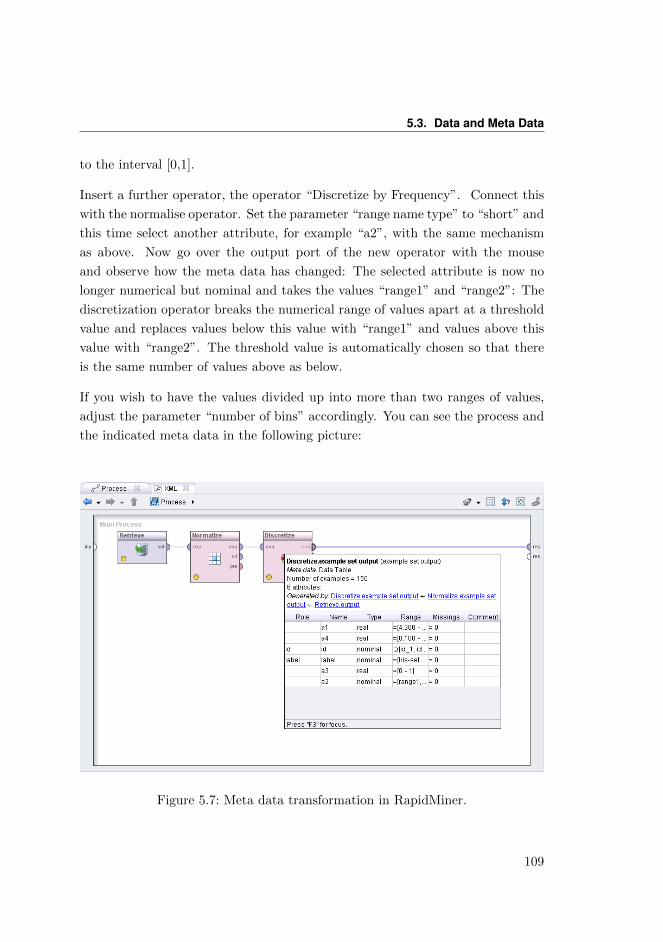
5.3. Data and Meta Data
to the interval [0,1].
Insert a further operator, the operator “Discretize by Frequency”. Connect this
with the normalise operator. Set the parameter “range name type” to “short” and
this time select another attribute, for example “a2”, with the same mechanism
as above. Now go over the output port of the new operator with the mouse
and observe how the meta data has changed: The selected attribute is now no
longer numerical but nominal and takes the values “range1” and “range2”: The
discretization operator breaks the numerical range of values apart at a threshold
value and replaces values below this value with “range1” and values above this
value with “range2”. The threshold value is automatically chosen so that there
is the same number of values above as below.
If you wish to have the values divided up into more than two ranges of values,
adjust the parameter “number of bins” accordingly. You can see the process and
the indicated meta data in the following picture:
Figure 5.7: Meta data transformation in RapidMiner.
109
5. Repository
You are surely wondering why the parameter “range name type” had to be set
to “short”. See for yourself and set it to “long”. If you execute the process, you
will see that the nominal values now give more information: They additionally
contain the limits of the intervals created. This is handy, but insignificant for the
process. The information on the interval limits is not available however as long
as the discretization has not actually been performed. Therefore it cannot be
considered for the meta data display at the time of process development. It can
then only be indicated in the meta data that the range of values of the discretized
attribute is a superset of the empty set i.e. that it is not empty. This means that
the meta data is not fully known. So in this case we can say virtually nothing
at all about the expected meta data, except that the set of nominal values is
a superset of the empty set. A trivial statement, but one that is nevertheless
correct. The meta data cannot be fully determined in all cases as early as at
the time of development. This is generally the case whenever the meta data is
dependent on the actual data as it is here. In this case RapidMiner Studio tries
to obtain as much information as possible about the data.
110


Global leader in predictive analytics software.Boston | London | Dortmund | Budapestwww.rapidminer.com