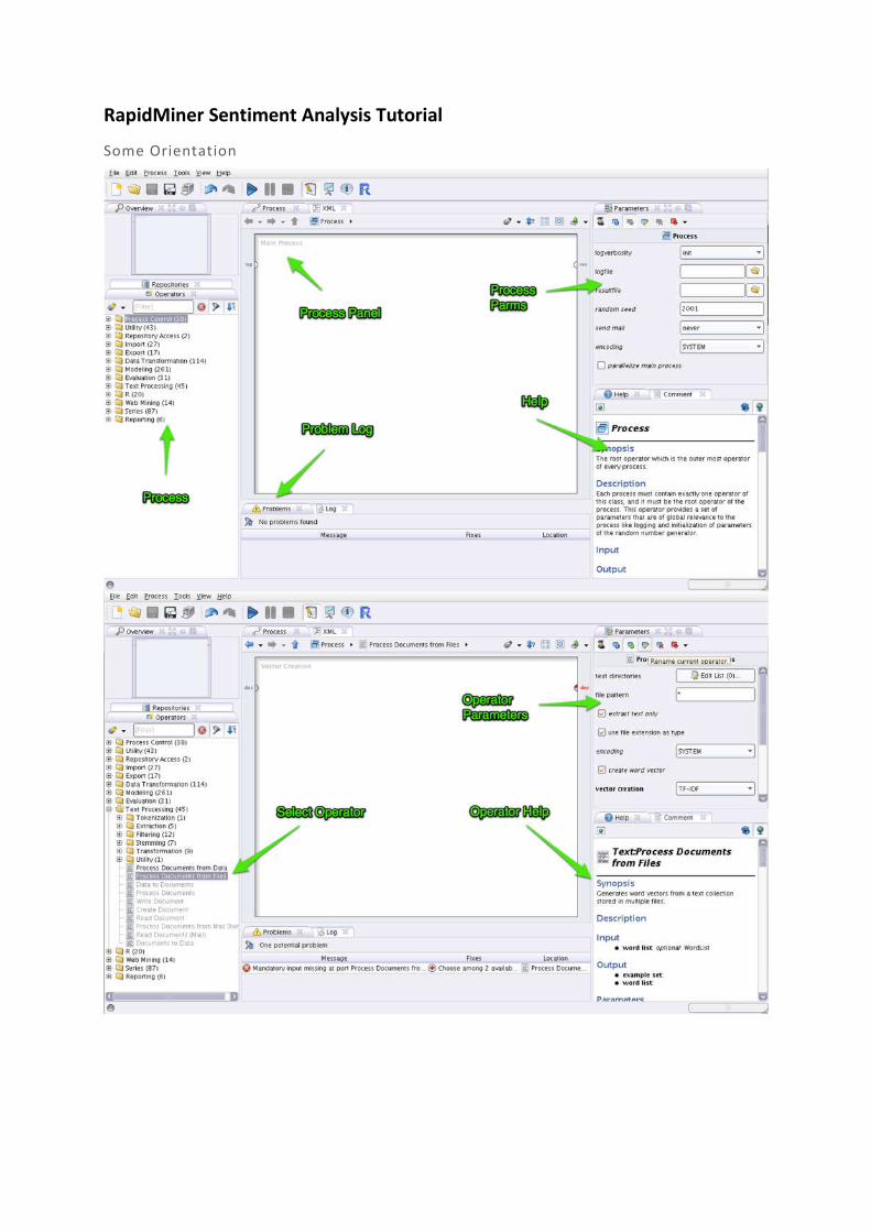
RapidMiner Sentiment Analysis Tutorial

Some Orientation

Set up Training

First make sure, that the TextProcessing Extensionis installed.

Retrieve labelled data: http://www.cs.cornell.edu/People/pabo/movie-review-data

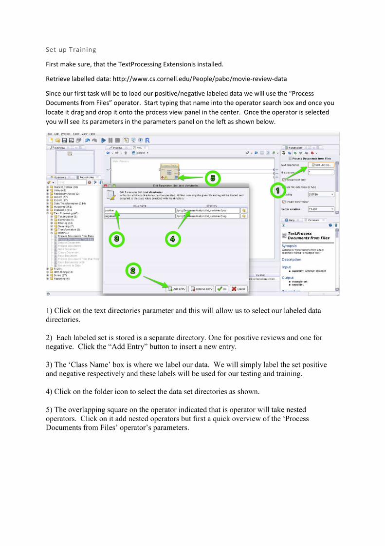
Since our first task will be to load our positive/negative labeled data we will use the “Process

Documents from Files” operator. Start typing that name into the operator search box and once you

locate it drag and drop it onto the process view panel in the center. Once the operator is selected

you will see its parameters in the parameters panel on the left as shown below.

1) Click on the text directories parameter and this will allow us to select our labeled data directories.

2) Each labeled set is stored is a separate directory. One for positive reviews and one for negative. Click the “Add Entry” button to insert a new entry.

3) The ‘Class Name’ box is where we label our data. We will simply label the set positive and negative respectively and these labels will be used for our testing and training.

4) Click on the folder icon to select the data set directories as shown.

5) The overlapping square on the operator indicated that is operator will take nested operators. Click on it add nested operators but first a quick overview of the ‘Process Documents from Files’ operator’s parameters.

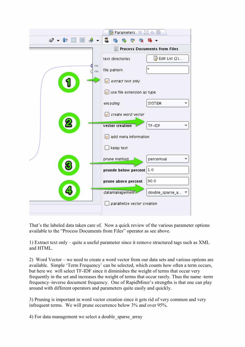
That’s the labeled data taken care of. Now a quick review of the various parameter options available to the “Process Documents from Files” operator as see above.

1) Extract text only – quite a useful parameter since it remove structured tags such as XML and HTML.

2) Word Vector – we need to create a word vector from our data sets and various options are available. Simple ‘Term Frequency’ can be selected, which counts how often a term occurs, but here we will select TF-IDF since it diminishes the weight of terms that occur very frequently in the set and increases the weight of terms that occur rarely. Thus the name -term frequency–inverse document frequency. One of RapidMiner’s strengths is that one can play around with different operators and parameters quite easily and quickly.

3) Pruning is important in word vector creation since it gets rid of very common and very infrequent terms. We will prune occurrence below 3% and over 95%.

4) For data management we select a double_sparse_array

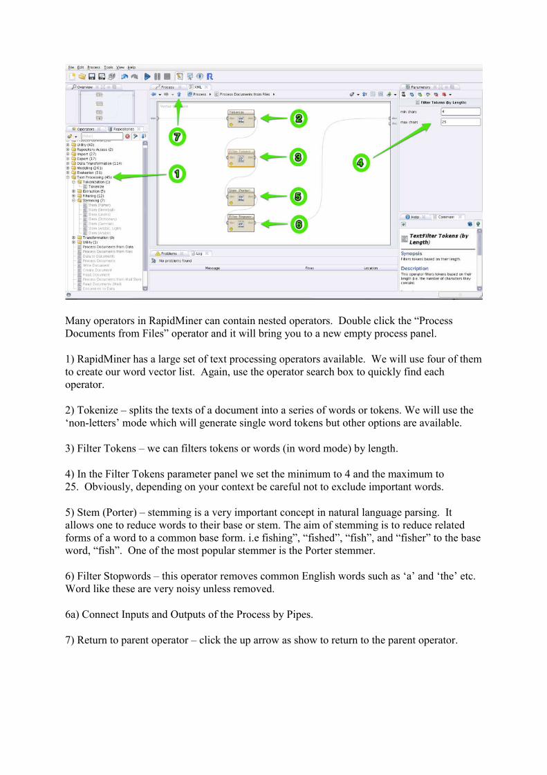
Many operators in RapidMiner can contain nested operators. Double click the “Process Documents from Files” operator and it will bring you to a new empty process panel.

1) RapidMiner has a large set of text processing operators available. We will use four of them to create our word vector list. Again, use the operator search box to quickly find each operator.

2) Tokenize – splits the texts of a document into a series of words or tokens. We will use the ‘non-letters’ mode which will generate single word tokens but other options are available.

3) Filter Tokens – we can filters tokens or words (in word mode) by length.

4) In the Filter Tokens parameter panel we set the minimum to 4 and the maximum to 25. Obviously, depending on your context be careful not to exclude important words.

5) Stem (Porter) – stemming is a very important concept in natural language parsing. It allows one to reduce words to their base or stem. The aim of stemming is to reduce related forms of a word to a common base form. i.e fishing”, “fished”, “fish”, and “fisher” to the base word, “fish”. One of the most popular stemmer is the Porter stemmer.

6) Filter Stopwords – this operator removes common English words such as ‘a’ and ‘the’ etc. Word like these are very noisy unless removed.

6a) Connect Inputs and Outputs of the Process by Pipes.

7) Return to parent operator – click the up arrow as show to return to the parent operator.

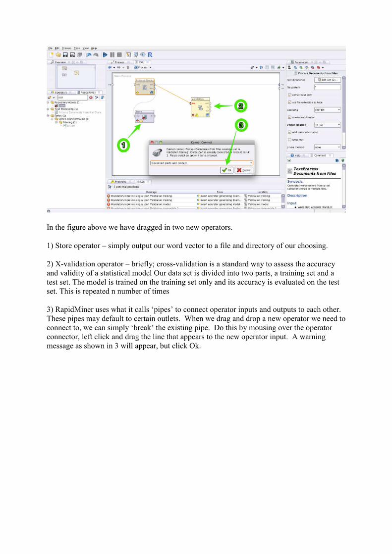
In the figure above we have dragged in two new operators.

1) Store operator – simply output our word vector to a file and directory of our choosing.

2) X-validation operator – briefly; cross-validation is a standard way to assess the accuracy and validity of a statistical model Our data set is divided into two parts, a training set and a test set. The model is trained on the training set only and its accuracy is evaluated on the test set. This is repeated n number of times

3) RapidMiner uses what it calls ‘pipes’ to connect operator inputs and outputs to each other. These pipes may default to certain outlets. When we drag and drop a new operator we need to connect to, we can simply ‘break’ the existing pipe. Do this by mousing over the operator connector, left click and drag the line that appears to the new operator input. A warning message as shown in 3 will appear, but click Ok.

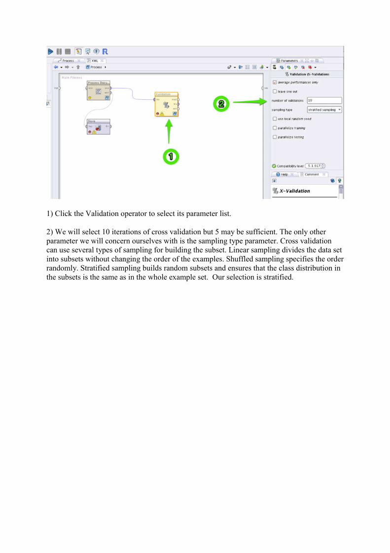
1) Click the Validation operator to select its parameter list.

2) We will select 10 iterations of cross validation but 5 may be sufficient. The only other parameter we will concern ourselves with is the sampling type parameter. Cross validation can use several types of sampling for building the subset. Linear sampling divides the data set into subsets without changing the order of the examples. Shuffled sampling specifies the order randomly. Stratified sampling builds random subsets and ensures that the class distribution in the subsets is the same as in the whole example set. Our selection is stratified.

Double click on the X-Validation operator and you’ll see a (1) training panel and a (2) testing panel.

In the figure above we populate the training and testing parts of our cross validator.

1) A popular set of classifier at the moment is Support Vector Machines ( SVMs), of which RapidMiner has several. We will use a linear SVM, one the simplest since the function is a linear combination of all the input variables.

2) Drag the SVM to the training panel. Note we could just have easily used another kind of classifier such as Naive Bayes or K-NN ( k nearest neighbor), all of which are available in RapidMiner. I’d encourage you to experiment with each of these especially since RapidMiner makes it so easy to do so.

3) The linear SVM has quite a few parameters, but we will use the defaults. The C parameter is the most important and represents the complexity constant. It specifies whether the model should be a more generalized model or a more specific model. The higher the C value the more impact an individual training example can have, thus leading to a more specific model. However, this may lead to over-fitting. One great feature of RapidMiner is an ‘Optimize Parameters’ parameter that can wrap an SVM and select the optimal parameters.

4) Now it’s time to test the model. First we will use the ‘Apply Model’ operator to apply the training set to our test set.

5) To measure the model accuracy we will use the ‘Performance (Binomial Classification)’ operator. Default settings are fine for both.

6) Connect the correct pipes: tra – tra Training Data, mod-mod-mod Trained Model, tes-unl Unlabelled Test Data, lab-lab Labelled Data, pre – ave Average Performance

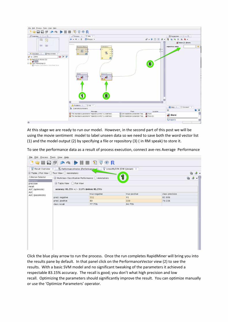
At this stage we are ready to run our model. However, in the second part of this post we will be

using the movie sentiment model to label unseen data so we need to save both the word vector list

(1) and the model output (2) by specifying a file or repository (3) ( in RM speak) to store it.

To see the performance data as a result of process execution, connect ave-res Average Performance

Click the blue play arrow to run the process. Once the run completes RapidMiner will bring you into

the results pane by default. In that panel click on the PerformanceVector view (2) to see the

results. With a basic SVM model and no significant tweaking of the parameters it achieved a

respectable 83.15% accuracy. The recall is good; you don’t what high precision and low

recall. Optimizing the parameters should significantly improve the result. You can optimize manually

or use the ‘Optimize Parameters’ operator.

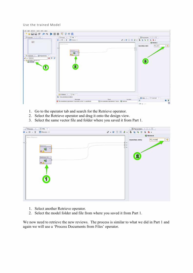
Use the trained Model

1. Go to the operator tab and search for the Retrieve operator. 2. Select the Retrieve operator and drag it onto the design view. 3. Select the same vector file and folder where you saved it from Part 1.

1. Select another Retrieve operator. 2. Select the model folder and file from where you saved it from Part 1.

We now need to retrieve the new reviews. The process is similar to what we did in Part 1 and again we will use a ‘Process Documents from Files’ operator.

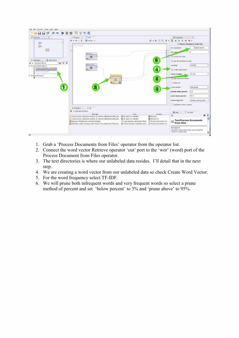
1. Grab a ‘Process Documents from Files’ operator from the operator list. 2. Connect the word vector Retrieve operator ‘out’ port to the ‘wor’ (word) port of the

Process Document from Files operator. 3. The text directories is where our unlabeled data resides. I’ll detail that in the next

step. 4. We are creating a word vector from our unlabeled data so check Create Word Vector. 5. For the word frequency select TF-IDF. 6. We will prune both infrequent words and very frequent words so select a prune

method of percent and set ‘below percent’ to 3% and ‘prune above’ to 95%.

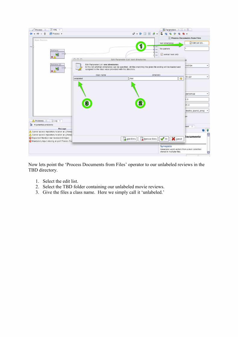
Now lets point the ‘Process Documents from Files’ operator to our unlabeled reviews in the TBD directory.

1. Select the edit list. 2. Select the TBD folder containing our unlabeled movie reviews. 3. Give the files a class name. Here we simply call it ‘unlabeled.’

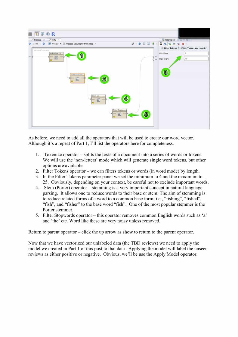
As before, we need to add all the operators that will be used to create our word vector. Although it’s a repeat of Part 1, I’ll list the operators here for completeness.

1. Tokenize operator – splits the texts of a document into a series of words or tokens. We will use the ‘non-letters’ mode which will generate single word tokens, but other options are available.

2. Filter Tokens operator – we can filters tokens or words (in word mode) by length. 3. In the Filter Tokens parameter panel we set the minimum to 4 and the maximum to

25. Obviously, depending on your context, be careful not to exclude important words. 4. Stem (Porter) operator – stemming is a very important concept in natural language

parsing. It allows one to reduce words to their base or stem. The aim of stemming is to reduce related forms of a word to a common base form; i.e., “fishing”, “fished”, “fish”, and “fisher” to the base word “fish”. One of the most popular stemmer is the Porter stemmer.

5. Filter Stopwords operator – this operator removes common English words such as ‘a’ and ‘the’ etc. Word like these are very noisy unless removed.

Return to parent operator – click the up arrow as show to return to the parent operator.

Now that we have vectorized our unlabeled data (the TBD reviews) we need to apply the model we created in Part 1 of this post to that data. Applying the model will label the unseen reviews as either positive or negative. Obvious, we’ll be use the Apply Model operator.

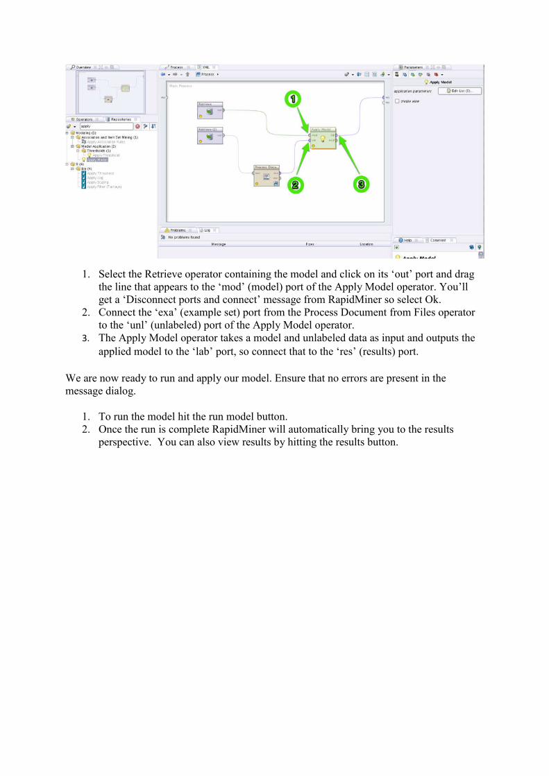
1. Select the Retrieve operator containing the model and click on its ‘out’ port and drag the line that appears to the ‘mod’ (model) port of the Apply Model operator. You’ll get a ‘Disconnect ports and connect’ message from RapidMiner so select Ok.

2. Connect the ‘exa’ (example set) port from the Process Document from Files operator to the ‘unl’ (unlabeled) port of the Apply Model operator.

3. The Apply Model operator takes a model and unlabeled data as input and outputs the applied model to the ‘lab’ port, so connect that to the ‘res’ (results) port.

We are now ready to run and apply our model. Ensure that no errors are present in the message dialog.

1. To run the model hit the run model button. 2. Once the run is complete RapidMiner will automatically bring you to the results

perspective. You can also view results by hitting the results button.