rapcer 01-18 - stefancollignon.de · stefan collignon, gianluca cubadda, giuseppe de arcangelis,...
TRANSCRIPT

Rapporto CER
Re-inventing Europe
n.1 2018


CENTRO EUROPA RICERCHE
ER produces short and medium-term forecast of the Italian economy, evalua-
tions on economic policy, reports on public finance, fiscal, monetary and industrial policy.
CER is regularly invited to auditions by the Italian Parliament on the economic outlook and
public finance trends. CER prepares a «consensus forecast» for the Italian Ministry of the
Economy jointly with other research institutes.
CER's forecasting and simulation expertise is embodied in its econometric models, which
are continuously updated to take into account structural changes in the national and in-
ternational economy. The econometric models are used to test the impact of policy
measures as well as provide forecasts of economic and financial variables.
The micro-simulation model, using data on wages and consumer expenditure, is used to
evaluate the distribution impact of tax and tariff measures on Italian households.
CER's reports are available to subscribers as are presentations and workshops on the reports
organised and sponsored by CER and attended to by experts and leading personalities
and policy makers.

Centro Europa Ricerche S.r.l.
Via G. Carissimi, 41 - 00198 Roma
Tel. (0039) 06 8081304
E-mail: [email protected]
www.centroeuroparicerche.it
Presidente Onorario: Giorgio Ruffolo
Presidente: Vladimiro Giacché
Vicepresidenti: Claudio Levorato, Gennaro Mariconda
Direttore della ricerca: Stefano Fantacone
Comitato scientifico: Paolo Guerrieri Paleotti (presidente), Barbara Annicchiarico, Pierluigi Ciocca,
Stefan Collignon, Gianluca Cubadda, Giuseppe De Arcangelis, Flavio Delbono, Francesco Ferrante,
Giovanni Ferri, Luca Fiorito, Sergio Ginebri, Paolo Giordani, Anna Giunta, Pasquale Lelio Iapadre, Mas-
similiano Marzo, Valentina Meliciani, Salvatore Nisticò, Antonio Pedone, Andrea Cesare Resti, Gio-
vanna Vallanti
Rapporto CER: pubblicazione periodica a carattere economico. Anno XXXV
Direttore responsabile: Jacopo Tondelli
Iscrizione n. 59/2016 del 5 aprile 2016 del Registro della Stampa del Tribunale di Roma
Proprietario della testata: Centro Europa Ricerche S.r.l.
C.C.I.A.A. Roma: R.E.A. 480286
Edizione: Centro Europa Ricerche S.r.l.
Printed out at CER – May, 2018

Re- invent ing Europe

The fol lowing authors have contributed to this report: Stefan Col l ignon,
Stefano Fantacone, Antonio Forte, Chiara Guerel lo.

R A P P O R T O C E R
5 5
Executive summary 7
The return of economic growth in Europe
11
UNEMPLOYMENT 13
PRODUCTIVITY GAPS 15
WAGE COST COMPETITIVENESS 17
Box 1. Non-TFP growth and output-gap 20
Policy mix
21
THE INTERACTION OF MONETARY AND FISCAL POLICY 21
MONETARY POLICY 25
FISCAL POLICY 28
EMPIRICAL EVIDENCE ON THE INTERACTION OF MONETARY AND FISCAL POLICY 32
Box 2. Fiscal-monetary policy mix in theory 36
Box 3. The ECB unconventional monetary stance 38
Box 4. Glossary for fiscal policy terms 39
European Fiscal Union
41
FISCAL POLICY COORDINATION IN THE EURO AREA 41
THE FLOW OF FUNDS ANALYSIS 43
Box 5. The current debate on fiscal spill-overs in the Euro Area 50
Towards a European Fiscal Union
51
THE EUROPEAN UNION BUDGET 52
A EUROPEAN FISCAL UNION FOR MACROECONOMIC STABILITY 55
References
57


R A P P O R T O C E R
7 7
Executive summary
President Macron has called for the re-invention of Europe. “Faced with the great chal-
lenges of our times, such as defence and security, great migrations, development, climate
change, the digital revolution and regulation of a globalized economy”, he asked, “have
European countries found means to defend their interests and values, and to guarantee
and adapt their democratic and social model that is unique worldwide? Can they address
each of these challenges alone? We cannot afford to keep the same policies, the same
habits, the same procedures and the same budget. No more can we choose to turn in-
wards within national borders. The only way to ensure our future, is the rebuilding of a sov-
ereign, united and democratic Europe” (1).
This year’s Rapporto Europa will focus on the economic context for re-inventing European
model. We give particular attention to the details of a European Fiscal Union. The Maas-
tricht Treaty did not incorporate any form of Fiscal Union, except in the very narrow sense
of fiscal discipline: each member state committed to maintain sound finances and the
Stability and Growth Pact (SGP) detailed the operationalisation of fiscal discipline. A com-
mon European budget exists, but it is small and has no specific functions for the Euro Area.
The Euro crisis has revealed that this institutional set-up is not optimal.
In June 2015, the so-called Five Presidents’ Report noted that “all mature Monetary Unions
have put in place a common macroeconomic stabilisation function to better deal with
shocks that cannot be managed at the national level alone” (p. 14). It proposed a “fiscal
union” that would “improve the cushioning of large macroeconomic shocks and thereby
make EMU over all more resilient” (p.14) (2).
Since then, many improvements have happened:
1. By the European Semester of economic policy coordination has been given clearer
guidance for the Euro Area as a whole and a stronger focus on social aspects.
2. European Fiscal Boards and National Productivity Boards have been set up.
3. Technical assistance to Member States was boosted with the creation of the Structural
Reform Support Service.
4. Important steps towards completing the Banking Union and Capital Markets Union
have been taken, notably by advancing in parallel on risk-reduction and risk-sharing
measures in the banking sector.
(1) http://www.elysee.fr/assets/Initiative-for-Europe-a-sovereign-united-democratic-Europe-Emmanuel-
Macron.pdf
(2) Juncker J‐C., D. Tusk, J. Dijsselbloem, M. Draghi and M. Schulz (2015): Completing Europe’s Economic
and Monetary Union, Five Presidents’ Report, 22 June. https://ec.europa.eu/commission/publica-
tions/five-presidents-report-completing-europes-economic-and-monetary-union_en

N. 1 - 2 0 1 8
8
In December 2017, the European Commission has presented new proposals and initiatives
that echoed President Macron’s discourse and Commission President Junker’s State of the
Union speech:
1. A European Monetary Fund (EMF) is to safeguard the financial stability of the Euro
Area, as well as the financial stability of the 'participating member states'
2. The so-called Fiscal compact (Treaty on Stability, Coordination and Governance) is to
be integrated into the Union legal framework, taking into account the appropriate
flexibility.
3. New budgetary instruments for the Euro Area are to be developed within the Union
framework.
4. For the period 2018-2020, EU funds will be mobilised in support of national reforms and
the Structural Reform Support Programme is to be strengthened.
5. Finally, reflection has started whether the Euro Area needs a European Minister of
Economy and Finance.
The interaction between sovereign member states’ fiscal policy and the unified monetary
policy is not optimal in the European Monetary Union (EMU). Therefore, the European Cen-
tral Bank is overcharged and the policy mix in the Euro Area has been suboptimal for a
long time. We believe that a European Fiscal Union will help to improve the policy mix and,
therefore, the long run development of the member states in the Euro Area. We develop
the analysis in this year’s Rapporto Europa starting from an overview of the main develop-
ments of the Euro Area economies. We then look at the economic governance of the Euro
Area, especially the coordination of fiscal policy between member states and the interac-
tion with monetary policy.
Economic activity is now well above the previous peak attained in 2008: it is 7.5% higher in
the Euro Area as a whole. Not only actual, but also potential output growth has improved
since the ECB has started its unconventional monetary policy in 2012. While this was a nec-
essary policy response to the crisis, the situation now calls for a cautious normalization of
monetary policy and a careful evaluation of fiscal policy.
The closing of the output gaps may explain why potential output is improving again across
Europe. Although the impact of closing the output gap on non-TFP growth differentials is
small, the indirect effect that output gaps exert on potential output growth through the
growth of factors of production is large. However, as the gaps disappear, one must con-
sider that in the long-run economic growth is determined by total factor productivity (TFP).
For stagnating countries like Italy, the challenge does not so much consist in stimulating the
economy, which could of course contribute to an increase in the use of capital and labour,
but more importantly structural reforms are urgently needed to improve the efficiency of
resource use and raise TFP. This is also necessary in order to improve competitiveness and
raise the purchasing power of wages.

R A P P O R T O C E R
9 9
Between 2011 and 2014, fiscal consolidation made the policy mix excessively tight; after
2014, monetary policy has contributed to a significant softening (real long-term interest
rates fell), but fiscal policy remained stuck at an aggregated cyclically adjusted deficit of
-1%. This aggregate development is not fully reflected in the levels of individual member
states’ real long-term interest rates: while in Italy nominal interest rates strongly declined,
the deflationary pressures shrank the gap between nominal and real interest rates, but in
Germany this gap widened, driving real interest rates into negative territory for several
years. The divergence in the real long-term interest rates’ dynamic observed in the last
years might be attributable to country-specific policy, and in particular to heterogeneous
fiscal stance. Before the crisis the relationship between long-term interest rate and the fiscal
stance was linear and negative across the countries, but during the crises and even more
recently this relationship has become highly non-linear.
We show that the government budget position does not explain the output gap, nor is the
volatility in government budgets affected by output gap volatility over the medium run. By
contrast, monetary policy is highly significant, confirming the excessive burden for
monetary policy in the European policy mix. However, monetary policy affects real long
run interest rates in the short-run, although in the medium run their dynamics depends also
on government budget positions. This highlights that the effectiveness of monetary policy
is highly dependent on the fiscal policy stance in shaping the dynamic of the long-run rate.
Since fiscal policies are heterogenous among the countries, the effectiveness of monetary
policy in stimulating the economy is highly uneven across countries.
Fiscal policies by member states are not neutral in the European monetary union, because
the changes of fiscal stances will generate spillover effects in neighbouring member states.
Our estimations suggest that signs and dimensions of spillovers are strongly hetoregeneous
among member countries so that a different form of fiscal policies coordination within the
Euro Area, defined by a strategic interaction between member countries on the timing of
consolidation, would be preferable to just a common set of rules, which might induce all
countries to consolidate at the same moment, making austerity unsustainable. However,
since the cross-country heterogeneity of attitude towards a joint consolidation across
country is a matter of fact, supranational coordination by means of a European Minister of
Finance might mediate this position, increasing the sustainability of fiscal consolidation in
Europe.
The budget of the European Union pays for policies carried out at the European level. The
total budget amounted to € 136 bln in 2016, which is less than 1% of gross national income
(GNI) of the European Union. Of this amount, € 117.9 bln are spend inside the EU but only €
77.2 bln in the Euro Area. There are therefore good reasons for increasing the budget for
the monetary union, as President Macron has demanded.
The experience has proven that the voluntary cooperation among the EU member states
is no longer sufficient to generate and allocate European public goods efficiently. Instead

N. 1 - 2 0 1 8
10
of intergovernmental cooperation, it may be a better solution to provide certain public
goods by a federal agency, which is acting on the basis of competing legislation. With
these elements, a re-invented European Union would be able to keep its founding promise:
namely to preserve peace, increase welfare and bring people together.

R A P P O R T O C E R
11 11
The return of economic growth in Europe
After a decade of economic recession, stagnation and crisis, Europe has finally returned
to solid economic growth. The recovery is part of a worldwide trend (IMF, 2018). Global
output has grown by 3.7% in 2017, and global growth forecasts for 2018 and 2019 have
been revised upward to 3.9%. The pickup in growth is broad-based, reflecting also upside
surprises in Europe and Asia and the expected impact of the recently approved U.S. tax
policy changes.
Economic activity, measured by GDP at constant prices, is now well above the previous
peak attained in 2008: it is 7.5% higher in the Euro Area as a whole. Contrary to the short-
lived export led economic revival in 2011, the present European recovery is fed by domes-
tic demand and has spread across countries and sectors. Figure 1 shows in the left panel
that in the Euro Area output is getting close to its potential and in the right panel that the
output gap has closed. This means that the recessionary tendencies and deflationary risks
are subsiding, while there are still no excessive demand pressures which could ignite a
wage-price inflation. The right-hand panel in Figure 1 also shows that not only actual, but
also potential output growth has improved since the European Central Bank has started its
unconventional monetary policy in 2012. While this was a necessary policy response to the
crisis, the situation now calls for a cautious normalization of monetary policy and a careful
evaluation of fiscal policy. However, the recent economic progress is not equally distrib-
uted. In Germany, GDP is 13.4% above its 2008 level, in France 8.6%, in Spain 4.3%, but it is
still -3.2% below that level in Italy and even -23.0% in Greece.
Figure 1. Economic activity and growth in the Euro Area
Source: European Commission AMECO database.
5000
5500
6000
6500
7000
7500
8000
8500
9000
9500
10000
10500
2000 2002 2004 2006 2008 2010 2012 2014 2016
-4
-2
0
2
4
6
8
Euro Area
Output Gap Real GDP Potential GDP
2000 2002 2004 2006 2008 2010 2012 2014 2016
-5%
-4%
-3%
-2%
-1%
0%
1%
2%
3%
4%
5%
Euro Area
Real GDP Growth Rate Potential GDP Growth Rate

N. 1 - 2 0 1 8
12
Figure 2 shows that Germany quickly closed the output gap after 2009, but potential
growth only improved after 2012, the year of aggressive monetary loosening. In France,
the output gap is still negative and potential output growth has nearly halved from 2% in
2000 to 1.2% in 2018, although the tendency is rising again. In Italy, the situation is far worse.
The output gap has been nearly double of France, and potential growth has been nega-
tive in every year from 2009 to 2016. In 2017 it turned positive with 0.3%. Thus, Italian living
conditions have deteriorated in absolute and relative terms. Nevertheless, Spain is an ex-
ample that not all of the South is doom and gloom: the output gap was larger than in Italy,
but potential output is now growing again and with 2.3% this is faster than in 2008. The worst
case is Greece, where the output gap is still large and potential output still falling.
Figure 2. Economic activity and growth in selected Member States
1000
1200
1400
1600
1800
2000
2200
2400
2600
2800
3000
2000 2002 2004 2006 2008 2010 2012 2014 2016
-6
-4
-2
0
2
4
6
Germany
Output Gap Real GDP Potential GDP
2000 2002 2004 2006 2008 2010 2012 2014 2016
-8%
-6%
-4%
-2%
0%
2%
4%
6%
Germany
Real GDP Growth Rate Potential GDP Growth Rate
1000
1200
1400
1600
1800
2000
2200
2000 2002 2004 2006 2008 2010 2012 2014 2016
-4
-2
0
2
4
6
8
France
Output Gap Real GDP Potential GDP
2000 2002 2004 2006 2008 2010 2012 2014 2016
-4%
-3%
-2%
-1%
0%
1%
2%
3%
4%
5%
France
Real GDP Growth Rate Potential GDP Growth Rate
1000
1100
1200
1300
1400
1500
1600
1700
2000 2002 2004 2006 2008 2010 2012 2014 2016
-6
-4
-2
0
2
4
6
Italy
Output Gap Real GDP Potential GDP
2000 2002 2004 2006 2008 2010 2012 2014 2016
-6%
-4%
-2%
0%
2%
4%
6%
Italy
Real GDP Growth Rate Potential GDP Growth Rate

R A P P O R T O C E R
13 13
cont. Figure 2. Economic activity and growth in selected Member States
Source: European Commission AMECO database.
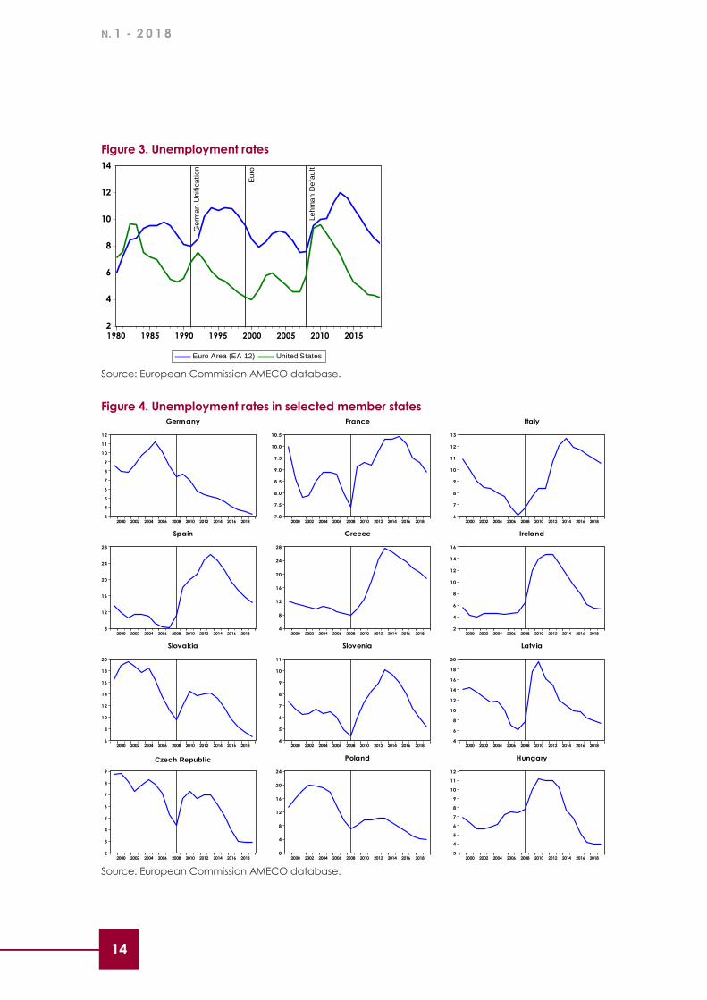
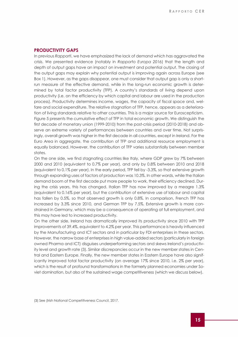
UNEMPLOYMENT
Unemployment is also coming down in Europe, although more slowly than in the US where
it is now at 4.3% - the lowest level since 2000 and the second lowest since 1970. As shown
in Figure 3, in the Euro Area, unemployment stood at 8.6% in 2018, still higher than at the
beginning of the Global Financial Crisis (7.5%), but below the level (9.7%) when monetary
union started in 1999. Thus, despite the severe crisis, it would be hard to argue that Europe
was better off without the euro.
Labour markets are improving in all member states (in the core as well as in the southern
periphery), although the levels are still diverging widely (see Figure 4). In Germany unem-
ployment stands at 3.5% of the labour force, in Ireland it has fallen from a peak of 14.5 to
5.5% and in Spain from 25.1 to 15.6%. Even in Greece, unemployment rates have come
down from 27.5 to 20.6%. Progress is slowest in Italy (10.9% down from 12.7%– still far above
the 6.8% before the crisis) and France (9.3% down from 10.4%). In the new member states,
unemployment rates stand between 7.7% (Latvia, Slovakia) and 2.9% (Czech Republic),
but in all Eastern member states they have come down by more than one half.
400
600
800
1000
1200
2000 2002 2004 2006 2008 2010 2012 2014 2016
-10
-5
0
5
10
15
Spain
Output Gap Real GDP Potential GDP
2000 2002 2004 2006 2008 2010 2012 2014 2016
-5%
-4%
-3%
-2%
-1%
0%
1%
2%
3%
4%
5%
6%
Spain
Real GDP Growth Rate Potential GDP Growth Rate
0
50
100
150
200
250
2000 2002 2004 2006 2008 2010 2012 2014 2016
-18
-9
0
9
18
27
Greece
Output Gap Real GDP Potential GDP
2000 2002 2004 2006 2008 2010 2012 2014 2016
-10%
-8%
-6%
-4%
-2%
0%
2%
4%
6%
8%
Greece
Real GDP Growth Rate Potential GDP Growth Rate
N. 1 - 2 0 1 8
14
Figure 3. Unemployment rates
Source: European Commission AMECO database.
Figure 4. Unemployment rates in selected member states
Source: European Commission AMECO database.
2
4
6
8
10
12
14
1980 1985 1990 1995 2000 2005 2010 2015
Euro Area (EA 12) United States
Ge
rma
n U
nif
ica
tio
n
Eu
ro
Le
hm
an
De
fau
lt
3
4
5
6
7
8
9
10
11
12
2000 2002 2004 2006 2008 2010 2012 2014 2016 2018
Germany
7.0
7.5
8.0
8.5
9.0
9.5
10.0
10.5
2000 2002 2004 2006 2008 2010 2012 2014 2016 2018
France
6
7
8
9
10
11
12
13
2000 2002 2004 2006 2008 2010 2012 2014 2016 2018
Italy
8
12
16
20
24
28
2000 2002 2004 2006 2008 2010 2012 2014 2016 2018
Spain
4
8
12
16
20
24
28
2000 2002 2004 2006 2008 2010 2012 2014 2016 2018
Greece
2
4
6
8
10
12
14
16
2000 2002 2004 2006 2008 2010 2012 2014 2016 2018
Ireland
6
8
10
12
14
16
18
20
2000 2002 2004 2006 2008 2010 2012 2014 2016 2018
Slovakia
4
5
6
7
8
9
10
11
2000 2002 2004 2006 2008 2010 2012 2014 2016 2018
Slovenia
4
6
8
10
12
14
16
18
20
2000 2002 2004 2006 2008 2010 2012 2014 2016 2018
Latvia
2
3
4
5
6
7
8
9
2000 2002 2004 2006 2008 2010 2012 2014 2016 2018
Czech Republic
0
4
8
12
16
20
24
2000 2002 2004 2006 2008 2010 2012 2014 2016 2018
Poland
3
4
5
6
7
8
9
10
11
12
2000 2002 2004 2006 2008 2010 2012 2014 2016 2018
Hungary
R A P P O R T O C E R
15 15
PRODUCTIVITY GAPS
In previous Rapporti, we have emphasized the lack of demand which has aggravated the
crisis. We presented evidence (notably in Rapporto Europa 2016) that the length and
depth of output gaps have an impact on investment and potential output. The closing of
the output gaps may explain why potential output is improving again across Europe (see
Box 1). However, as the gaps disappear, one must consider that output gap is only a short-
run measure of the effective demand, while in the long-run economic growth is deter-
mined by total factor productivity (TFP). A country’s standards of living depend upon
productivity (i.e. on the efficiency by which capital and labour are used in the production
process). Productivity determines income, wages, the capacity of fiscal space and, wel-
fare and social expenditure. The relative stagnation of TFP, hence, appears as a deteriora-
tion of living standards relative to other countries. This is a major source for Euroscepticism.
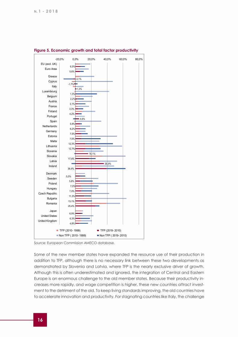
Figure 5 presents the cumulative effect of TFP in total economic growth. We distinguish the
first decade of monetary union (1999-2010) from the post-crisis period (2010-2018) and ob-
serve an extreme variety of performances between countries and over time. Not surpris-
ingly, overall growth was higher in the first decade in all countries, except in Ireland. For the
Euro Area in aggregate, the contribution of TFP and additional resource employment is
equally balanced. However, the contribution of TFP varies substantially between member
states.
On the one side, we find stagnating countries like Italy, where GDP grew by 7% between
2000 and 2010 (equivalent to 0.7% per year), and only by 0.8% between 2010 and 2018
(equivalent to 0.1% per year). In the early period, TFP fell by -3.3%, so that extensive growth
through expanding uses of factors of production was 10.3%. In other words, while the Italian
demand boom of the first decade put more people to work, their efficiency declined. Dur-
ing the crisis years, this has changed. Italian TFP has now improved by a meagre 1.3%
(equivalent to 0.16% per year), but the contribution of extensive use of labour and capital
has fallen by 0.5%, so that observed growth is only 0.8%. In comparison, French TFP has
increased by 3.3% since 2010, and German TFP by 7.5%. Extensive growth is more con-
strained in Germany, which may be a consequence of operating at full employment, and
this may have led to increased productivity.
On the other side, Ireland has dramatically improved its productivity since 2010 with TFP
improvements of 39.4%, equivalent to 4.2% per year. This performance is heavily influenced
by the Manufacturing and ICT sectors and in particular by FDI enterprises in these sectors.
However, the narrow base of enterprises in high value-added sectors (particularly in foreign
owned Pharma and ICT) disguises underperforming sectors and skews Ireland’s productiv-
ity level and growth rate (3). Similar discrepancies occur in the new member states in Cen-
tral and Eastern Europe. Finally, the new member states in Eastern Europe have also signif-
icantly improved total factor productivity (on average 17% since 2010, i.e. 2% per year),
which is the result of profound transformations in the formerly planned economies under So-
viet domination, but also of the sustained wage competitiveness (which we discuss below).
(3) See (Irish National Competitiveness Council, 2017.
N. 1 - 2 0 1 8
16
Figure 5. Economic growth and total factor productivity
Source: European Commission AMECO database.
Some of the new member states have expanded the resource use of their production in
addition to TFP, although there is no necessary link between these two developments as
demonstrated by Slovenia and Latvia, where TFP is the nearly exclusive driver of growth.
Although this is often underestimated and ignored, the integration of Central and Eastern
Europe is an enormous challenge to the old member states. Because their productivity in-
creases more rapidly, and wage competition is higher, these new countries attract invest-
ment to the detriment of the old. To keep living standards improving, the old countries have
to accelerate innovation and productivity. For stagnating countries like Italy, the challenge
6,5%
5,6%
-3,1%
-1,7%
1,3%
1,3%
2,2%
3,1%
3,3%
4,2%
4,6%
5,9%
6,2%
7,5%
7,5%
12,3%
12,7%
16,1%
17,4%
35,9%
39,4%
5,5%
5,8%
7,0%
7,0%
11,3%
13,1%
25,4%
6,9%
6,3%
4,8%
-20,0% 0,0% 20,0% 40,0% 60,0% 80,0%
EU (excl. UK)
Euro Area
Greece
Cyprus
Italy
Luxembourg
Belgium
Austria
France
Finland
Portugal
Spain
Netherlands
Germany
Estonia
Malta
Lithuania
Slovenia
Slovakia
Latvia
Ireland
Denmark
Sweden
Poland
Hungary
Czech Republic
Bulgaria
Romania
Japan
United States
United Kingdom
TFP (2010- 1999) TFP (2019- 2010)
Non TFP ( 2010- 1999) Non TFP ( 2019- 2010)
R A P P O R T O C E R
17 17
does not so much consist in stimulating the economy, which could of course contribute to
an increase in the use of capital and labour, but more importantly in improving the effi-
ciency of resource use and raise total factor productivity.
In the UK, productivity has slowed down. A major reason for this development is the uncer-
tainty for investors created by Brexit. A detailed study by the National Institute of Economic
and Social Research (Young, 2017) has shown that the UK’s standard of living are deterio-
rating because of higher cost of living due to the currency depreciation that weighs heavily
on the unemployed, single parents and pension holders. In addition, weak investment and
the delocalisation of businesses will have long run effects, which are already showing up
as a 20% reduction in the productivity trend.
WAGE COST COMPETITIVENESS
The unequal developments in productivity affect the competitiveness in the different re-
gions and member states of the Euro Area. In previous RAPPORTI, we have elaborated a
methodology for assessing the competitiveness of wage levels.
We have derived a benchmark wage level from the classic textbook assumption that equi-
librium in a single market would reflect equal returns on capital. Given the relative levels of
capital and labour productivity, we can derive from this assumption the equilibrium level
of wages at which this equal return would be realised. When the actual wage levels are
below the equilibrium, an economy is considered to be competitive, and inversely if actual
wages are higher, it lacks competitiveness. This means that the evolution of the equilibrium
wage is highly significant for the improvement of standards of living and this improvement
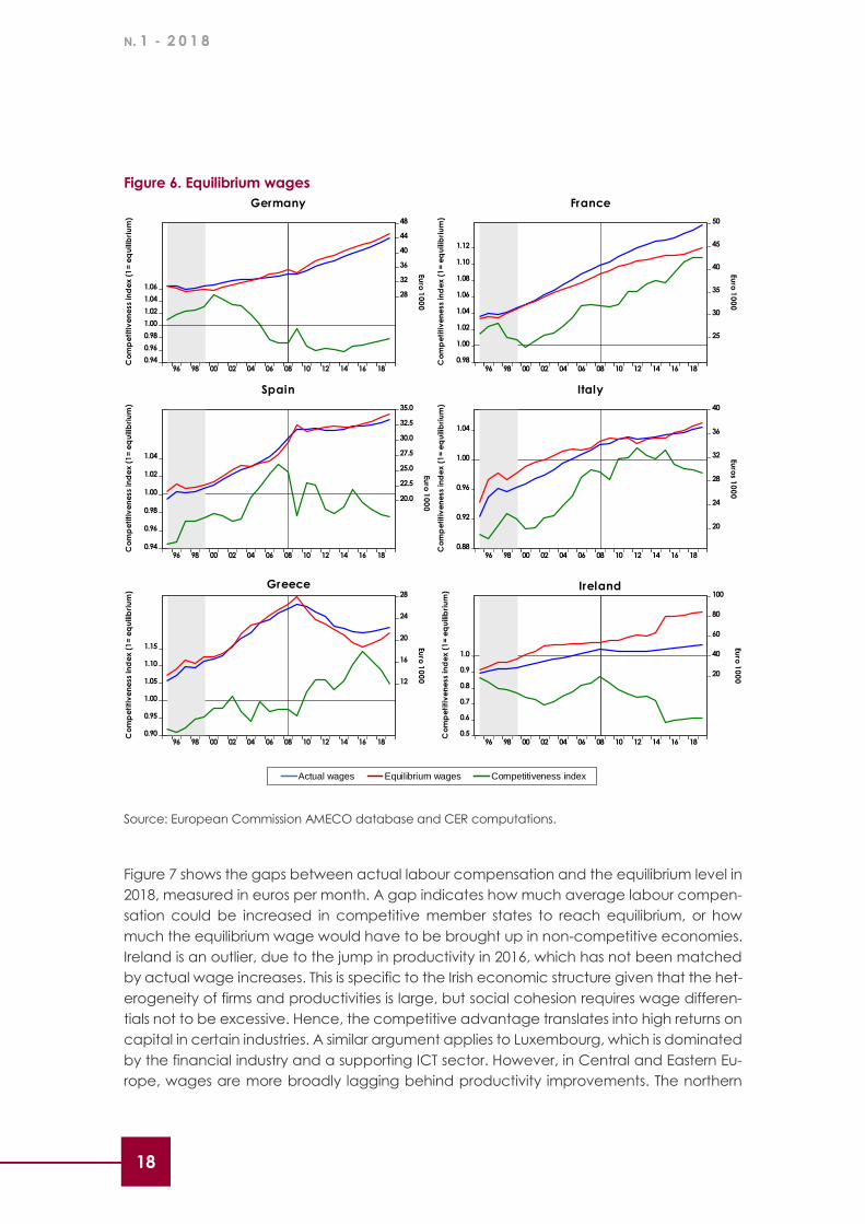
depends on the developments of productivity. Figure 6 shows the developments of actual
and equilibrium wages for selected Euro Area member states and Figure 7 shows the 2018
wage gaps for all member states in the European Union.
We find in Figure 6 that Germany has regained competitiveness since it undertook labour
market reforms in the mid-2000s, while France has persistently lost competitiveness with
wages today 10% above equilibrium. The loss was accelerated in 2015 when actual labour
compensation increased despite a stagnation in the equilibrium level. Since 2016 compet-
itiveness has improved in Italy and Spain. In Italy this seems to be the effect of the Job Act
of 2014-15. In Greece, the equilibrium wage has now started to rise after a sustained re-
duction before 2016, which was not compensated by the cuts in actual wage costs. In
Ireland, by contrast, we observe a significant leap in equilibrium wages, which is explained
by increases in productivity: “Across the OECD, labour productivity growth in manufactur-
ing has tended to outpace services sector growth. Between 2009 and 2015, Irish growth in
manufacturing was 16% compared with 3% in services and -2% in construction. Irish manu-
facturing productivity data has been significantly influenced by corporate restructuring
[…], including the relocation of firms with significant IP assets and aircraft leasing, [leading]
to noteworthy increases in labour productivity, particularly in 2015 (22.5%)” (Irish National
Competitiveness Council, 2017, pp. 58-62).
N. 1 - 2 0 1 8
18
Figure 6. Equilibrium wages
Source: European Commission AMECO database and CER computations.
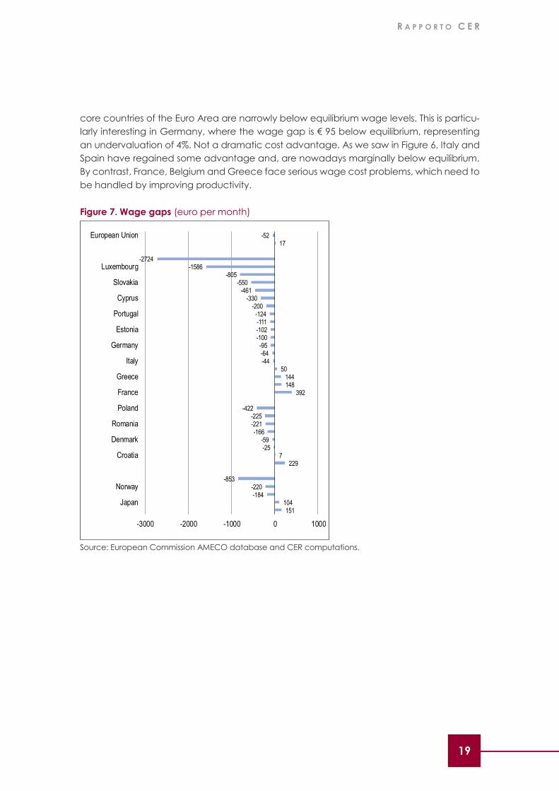
Figure 7 shows the gaps between actual labour compensation and the equilibrium level in
2018, measured in euros per month. A gap indicates how much average labour compen-
sation could be increased in competitive member states to reach equilibrium, or how
much the equilibrium wage would have to be brought up in non-competitive economies.
Ireland is an outlier, due to the jump in productivity in 2016, which has not been matched
by actual wage increases. This is specific to the Irish economic structure given that the het-
erogeneity of firms and productivities is large, but social cohesion requires wage differen-
tials not to be excessive. Hence, the competitive advantage translates into high returns on
capital in certain industries. A similar argument applies to Luxembourg, which is dominated
by the financial industry and a supporting ICT sector. However, in Central and Eastern Eu-
rope, wages are more broadly lagging behind productivity improvements. The northern
0.94
0.96
0.98
1.00
1.02
1.04
1.0628
32
36
40
44
48
96 98 00 02 04 06 08 10 12 14 16 18
Germany
Eu
ro 1
00
0
Co
mp
eti
tiv
en
ess in
de
x (
1=
eq
uili
bri
um
)
0.98
1.00
1.02
1.04
1.06
1.08
1.10
1.12
25
30
35
40
45
50
96 98 00 02 04 06 08 10 12 14 16 18
France
Co
mp
eti
tiv
en
ess in
de
x (
1=
eq
uili
bri
um
)
Eu
ro 1
00
0
0.94
0.96
0.98
1.00
1.02
1.04
20.0
22.5
25.0
27.5
30.0
32.5
35.0
96 98 00 02 04 06 08 10 12 14 16 18
Co
mp
eti
tiv
en
ess
ind
ex
(1
= e
qu
ilib
riu
m)
Spain
0.88
0.92
0.96
1.00
1.04
20
24
28
32
36
40
96 98 00 02 04 06 08 10 12 14 16 18
Italy
Co
mp
eti
tiv
en
ess
ind
ex
(1
= e
qu
ilib
riu
m)
Euro
s 10
00
0.90
0.95
1.00
1.05
1.10
1.15
12
16
20
24
28
96 98 00 02 04 06 08 10 12 14 16 18
Co
mp
eti
tiv
en
ess
ind
ex
(1
= e
qu
ilib
riu
m)
Euro
10
00
Greece
0.5
0.6
0.7
0.8
0.9
1.0
20
40
60
80
100
96 98 00 02 04 06 08 10 12 14 16 18
Act ual w ages Equilibrium wages Comet it iveness index
Ireland
Co
mp
eti
tiv
en
ess
ind
ex
(1
= e
qu
ilib
riu
m)
Euro
10
00
Euro
10
00
0
50
100
150
200
250
300
Titolo del grafico
Actual wages Equilibrium wages Competitiveness index
R A P P O R T O C E R
19 19
core countries of the Euro Area are narrowly below equilibrium wage levels. This is particu-
larly interesting in Germany, where the wage gap is € 95 below equilibrium, representing
an undervaluation of 4%. Not a dramatic cost advantage. As we saw in Figure 6, Italy and
Spain have regained some advantage and, are nowadays marginally below equilibrium.
By contrast, France, Belgium and Greece face serious wage cost problems, which need to
be handled by improving productivity.
Figure 7. Wage gaps (euro per month)
Source: European Commission AMECO database and CER computations.
-5217
-2724-1586
-805-550
-461-330
-200-124-111-102-100-95-64-44
50144148
392
-422-225-221-166
-59-25
7229
-853-220-184
104151
-3000 -2000 -1000 0 1000
European Union
Luxembourg
Slovakia
Cyprus
Portugal
Estonia
Germany
Italy
Greece
France
Poland
Romania
Denmark
Croatia
Norway
Japan
N. 1 - 2 0 1 8
20
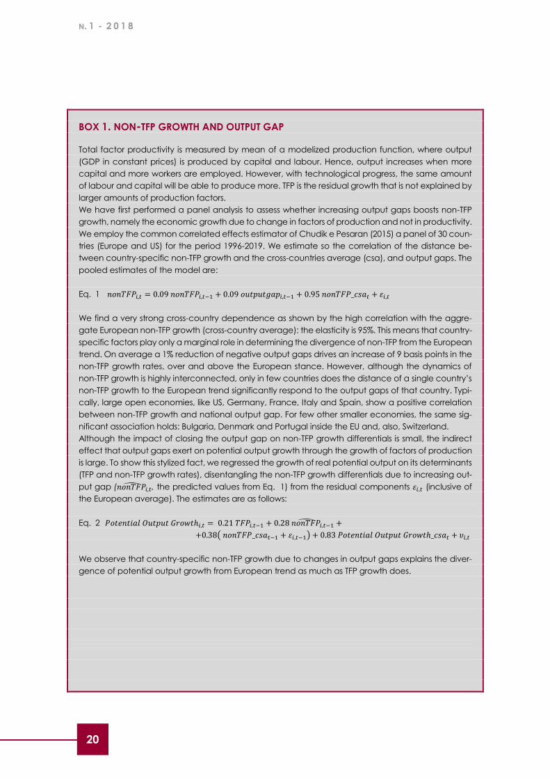
BOX 1. NON-TFP GROWTH AND OUTPUT GAP
Total factor productivity is measured by mean of a modelized production function, where output
(GDP in constant prices) is produced by capital and labour. Hence, output increases when more
capital and more workers are employed. However, with technological progress, the same amount
of labour and capital will be able to produce more. TFP is the residual growth that is not explained by
larger amounts of production factors.
We have first performed a panel analysis to assess whether increasing output gaps boosts non-TFP
growth, namely the economic growth due to change in factors of production and not in productivity.
We employ the common correlated effects estimator of Chudik e Pesaran (2015) a panel of 30 coun-
tries (Europe and US) for the period 1996-2019. We estimate so the correlation of the distance be-
tween country-specific non-TFP growth and the cross-countries average (csa), and output gaps. The
pooled estimates of the model are:
Eq. 1 𝑛𝑜𝑛𝑇𝐹𝑃𝑖,𝑡 = 0.09 𝑛𝑜𝑛𝑇𝐹𝑃𝑖,𝑡−1 + 0.09 𝑜𝑢𝑡𝑝𝑢𝑡𝑔𝑎𝑝𝑖,𝑡−1 + 0.95 𝑛𝑜𝑛𝑇𝐹𝑃_𝑐𝑠𝑎𝑡 + 𝜀𝑖,𝑡
We find a very strong cross-country dependence as shown by the high correlation with the aggre-
gate European non-TFP growth (cross-country average): the elasticity is 95%. This means that country-
specific factors play only a marginal role in determining the divergence of non-TFP from the European
trend. On average a 1% reduction of negative output gaps drives an increase of 9 basis points in the
non-TFP growth rates, over and above the European stance. However, although the dynamics of
non-TFP growth is highly interconnected, only in few countries does the distance of a single country’s
non-TFP growth to the European trend significantly respond to the output gaps of that country. Typi-
cally, large open economies, like US, Germany, France, Italy and Spain, show a positive correlation
between non-TFP growth and national output gap. For few other smaller economies, the same sig-
nificant association holds: Bulgaria, Denmark and Portugal inside the EU and, also, Switzerland.
Although the impact of closing the output gap on non-TFP growth differentials is small, the indirect
effect that output gaps exert on potential output growth through the growth of factors of production
is large. To show this stylized fact, we regressed the growth of real potential output on its determinants
(TFP and non-TFP growth rates), disentangling the non-TFP growth differentials due to increasing out-
put gap (𝑛𝑜𝑛𝑇𝐹𝑃̂𝑖,𝑡, the predicted values from Eq. 1) from the residual components 𝜀𝑖,𝑡 (inclusive of
the European average). The estimates are as follows:
Eq. 2 𝑃𝑜𝑡𝑒𝑛𝑡𝑖𝑎𝑙 𝑂𝑢𝑡𝑝𝑢𝑡 𝐺𝑟𝑜𝑤𝑡ℎ𝑖,𝑡 = 0.21 𝑇𝐹𝑃𝑖,𝑡−1 + 0.28 𝑛𝑜𝑛𝑇𝐹𝑃̂𝑖,𝑡−1 +
+0.38( 𝑛𝑜𝑛𝑇𝐹𝑃_𝑐𝑠𝑎𝑡−1 + 𝜀𝑖,𝑡−1) + 0.83 𝑃𝑜𝑡𝑒𝑛𝑡𝑖𝑎𝑙 𝑂𝑢𝑡𝑝𝑢𝑡 𝐺𝑟𝑜𝑤𝑡ℎ_𝑐𝑠𝑎𝑡 + 𝜐𝑖,𝑡
We observe that country-specific non-TFP growth due to changes in output gaps explains the diver-
gence of potential output growth from European trend as much as TFP growth does.

R A P P O R T O C E R
21 21
Policy mix
While long-run standards of living depend on productivity and supply side conditions, the
management of aggregate demand generates incentives for private investment and
growth. If these incentives are sustained over time, productivity and potential output will
rise. This is why a stability oriented macroeconomic policy framework is crucial for the per-
formance of the Euro Area economy. However, if different regions and sectors of produc-
tion respond with different elasticities to demand impulses, economic growth will diverge,
generating inequalities which might cause political backlashes. This is an important argu-
ment in favour of more coordinated economic policies in Europe.
The Euro Area has a unique set of policy rules and institutions, which makes policy coordi-
nation difficult. Monetary policy is centralized by the independent European Central Bank,
while fiscal and economic policy is decentralized in the hands of sovereign member states,
which are, however, constrained by a set of rules such as the Stability and Growth Pact
and the new Fiscal Compact. These rules do not apply to the same extend to member
states outside the Euro Area. However, experience of the Euro crisis has shown that the
interaction between monetary policy and fiscal policy, i.e. the policy mix, has not been
satisfactory. Fiscal policy was excessively rigid, while the European Central Bank has done
its utmost to save the euro and stimulate the euro economy. This sub-optimal performance,
which risks undermining the credibility of the ECB, has been widely recognized. It has given
rise to calls for a European Fiscal Union. Before analysing the effects of fiscal policy in detail,
we will first discuss the experience of the policy mix during the crisis.
THE INTERACTION OF MONETARY AND FISCAL POLICY
About the interaction of monetary and fiscal policies there is an abundance of literature
(4). Monetary policy refers to the central bank’s control of the availability of credit in the
economy to achieve the broad objectives of economic policy. Fiscal policy refers to the
government’s choice regarding the use of taxation and public spending to regulate the
aggregate level of economic activity. This is also called the stabilisation function of public
finance. Its purpose is to avoid excess demand pressures, which would cause inflation, and
lack of aggregate demand which would cause recessions and unemployment. Thus, the
output gap is a good proxy for measuring whether the stability objective is attained.
Because total public expenditure in the Euro Area is around 45% of GDP, the role of public
spending is of prime importance for the performance of aggregate demand. Yet, given
the independence of sovereign member states, each government can decide its own
budget, so that the aggregate budget position for the Euro Area is the random outcome
of national decisions. This means fiscal policy cannot be used as a policy instrument, and
as a consequence the full burden of managing the macroeconomic conditions in the Euro
Area falls on the European Central Bank. However, while the ECB can respond to an ag-
(4) For a review see (Hilbers, 2005) and (Fores, 2018).

N. 1 - 2 0 1 8
22
gregate shock to the Euro Area as a whole, it does not have instruments to manage asym-
metric shocks which translate into unequal output gaps between member states.
This is true for all integrated monetary economies, but in traditional nation states govern-
ments can use public finances to avoid or correct excessive deviations. Of course, eco-
nomic liberals are opposed to the interference by governments in the market, because
they believe the “invisible hand of the market” mechanism will restore equilibrium. How-
ever, our analysis of wage competitiveness shows that this adjustment process may take
longer than is politically acceptable. The populist alternative is to exit monetary union and
the single market. However, even if it were possible to do so without serious welfare losses
(which is not true) (5), this does not solve the fundamental economic problem in any inte-
grated currency union. Because substantial economic heterogeneities prevail, logically
northern Italy should also break away from monetary union with the Mezzogiorno, West
Germany from East Germany, Catalonia from Spain, and Flanders from Wallonia. Robert
Mundell, who was awarded the Nobel Prize for his work on optimum currency areas, has
therefore always argued that monetary union is a political project and not an economic
optimum. But this implies that a well-working monetary union requires a fiscal union with
additional policy tools and ultimately also a political union.
Thus, although monetary and fiscal policy are implemented by different bodies, these pol-
icies are far from independent. As explained in Box 2, a change in one will influence the
effectiveness of the other and thereby the overall impact of any policy change. Finding
the right policy mix is not always easy, but in the European Monetary Union the difficulty is
compounded by the fact that there is no federal authority to determine the aggregate
fiscal policy stance for the Euro Area.
Figure 9 gives an idea of the policy trade-off in the Euro Area. We have proxied monetary
policy by the long run real interest rates and fiscal policy by the cyclically adjusted struc-
tural deficits. The regression line, which stands for our efficiency line in Figure B2.1 of Box 2,
indicates that the long run real interest at balanced budgets would be 1.9%, which - in
“normal times” and given the inflation target of the ECB - is equivalent to a nominal long-
term rate of 3.9%. Given the historic record, this seems reasonable (see Figure 11).
Defining an optimal policy mix in the Euro Area poses a problem, because the aggregate
budget position which corresponds to the unified monetary policy stance is the sum of
different national government positions. Each national government has its own welfare
function and chooses its budget position in response to its national constituency. But if each
country is allowed to set its fiscal policy stance independently of the others, the conse-
quence will be that high deficits in some countries would push interest rates up for member
states with low deficits. Hence, national fiscal policies create externalities for all citizens in the
Euro Area. The resultant policy mix cannot be optimal. On the other hand, imposing a unique
policy stance for every government would create welfare losses because the policy prefer-
ences resulting from different welfare functions would be overwritten by the unique policy
rule. The Stability and Growth Pact effectively imposes a balanced budget at point E of Fig-
ure B2.1, where the indifference curve does not correspond with the policy preference of R.
(5) The National Institute (Young, 2017) has estimated that the first 18 months since the Brexit vote have
created costs “worth over £600 per annum to the average household” in the UK.

R A P P O R T O C E R
23 23
Figure 9. Policy mix in the Euro Area
Source: European Commission AMECO database.
The problem is partly economic, partly political. It is economic if the response of the eco-
nomic system to a fiscal deficit is significantly different from the Euro Area average. There
is evidence, discussed below, that the single currency has endogenously generated con-
vergence to a more unified economic response. However, as shown in Box 2, the political
problem remains unsolved, for example, at the balanced budget point E (Figure B2.1),
countries with a preference for point R remain on a lower level of utility. In a federal de-
mocracy the policy mix is chosen by all citizens through the democratic procedures of
electing a government. This means, there is only one collectively chosen welfare function,
which represents a democratic consensus. The point where such indifference curve
touches the efficiency line would therefore correspond to a welfare optimum. For exam-
ple, in the American context of the 1980s, the point R (for Republican) reflected the Volker-
Reagan policy mix, while the point E was closer to the Clinton Greenspan policy mix of the
1990s. In the European Union, where sovereign nation states are in command, such collec-
tive choice is not possible, and this undermines the perception of welfare gains in monetary
union. To overcome this problem, it would be desirable to find a form of policy coordina-
tion, which allows, on the one hand, the designation of a collective fiscal position that cor-
responds to the integrated monetary policy, and, on the other hand, that enables citizens’
representation in the conduct of fiscal policy. This would be the European equivalent of
the American slogan: “no taxation without representation”.
The most remarkable feature in Figure 9 is the complete absence of fiscal policy during the
Euro crisis. Fiscal consolidation between 2011 and 2014 made the policy mix excessively
tight: the points for those years are well above the equilibrium line. Finally, after 2014, mon-
etary policy contributed to a significant softening (real long-term interest rates fell verti-
cally), but fiscal policy remained stuck at an aggregated cyclically adjusted deficit of -1%.
No doubt, this was due to the fact that fiscal policy in the Euro Area is constrained by the
Stability and Growth Pact and the Fiscal Compact, which impose the identical rule of bal-
ancing cyclically adjusted deficits. We shall discuss this further below. Furthermore, in recent
years, budget positions have been quite heterogeneous across member states, while the
long-term interest rates had a tendency to decline. Figure 10 indicates the spread of na-
tional long- term interest rates in relation to the national deviation from the Euro Area fiscal
2010
2011
2012
2013
2014
2015
2016
y = -0,8631x - 0,1872R² = 0,7444
-0,5
0,0
0,5
1,0
1,5
2,0
2,5
3,0
3,5
4,0
-4,5 -4,0 -3,5 -3,0 -2,5 -2,0 -1,5 -1,0 -0,5 0,0
Rea
l Lon
g-Te
rm In
tere
ts R
ate
Structural Government Balance (% of potential GDP)

N. 1 - 2 0 1 8
24
stance. The scatterplot shows country-specific cyclically adjusted government budgets net
of interest (i.e. the distance from EA average) and the associated 10-year government
bond yield (distance from EA average) as the mean through the period 1999-2008 or 2009-
2017.
Figure 10. Correlation between fiscal stance and long-term interest rates
Source: European Commission AMECO database and ECB statistical data warehouse (SDW).
Before the financial crisis and the European sovereign crisis the relationship between long-
term interest rate and the fiscal stance was linear and negative. That means that if a
country under-consolidates (primary fiscal deficit higher than the Euro Area average), then
it would have paid a positive spread between the country’s long-term interest rate and the
Euro average one. This mechanism was called the market discipline, and it worked even if
it did not prevent the Euro crisis. By contrast, during the crises and even more recently this
relationship has become highly non-linear. This seems to be the result of the emergence of
four clusters. The spread of long-term interest rates over the average Euro rate was
negative for countries with fiscal consolidation, with the exception of Italy and Greece
(Greece being a large outlier, the data are not shown). These two countries have the
highest debt-GDP ratios in Europe and this explains why long-term bond yields contain
significant risk permia, so that even the strong fiscal consolidation does not bring the spread
down. However, another explanation would be that excessive austerity is
counterproductive because it increases market worries and uncertainty. This interpretation
is supported by the two other clusters in Figure 10. In Portugal, Cyprus, Latvia, and Lithuania
interest spreads remain high against a moderate fiscal losening. But in Spain, Slovakia,
Slovenia and France, the fiscal expansion goes together with a fall of long-term rates below
the Euro average, which makes sense if markets expect that the looser fiscal stance will
generate growth. Nevertheless, from the point of view of the Euro Area one could also
argue that this last cluster is free riding on the consolidation efforts by Germany, Luxemburg
and Italy.
BE
DE
FR
LV
LT
LU
MT
NLAT
SI
SK
FI
ES IT
CY
PT
BEDE IEES
FR
ITCYLV
LT
LU
MTNLAT
PT
SI
SK
y = 0,3135x3 - 0,4454x2 - 1,2962xR² = 0,4249
y = 0,0296x2 - 0,2722xR² = 0,4914
-2,5
-2,0
-1,5
-1,0
-0,5
0,0
0,5
1,0
1,5
2,0
2,5
-4,0 -3,0 -2,0 -1,0 0,0 1,0 2,0 3,0 4,0 5,0 6,0
Lo
ng
-te
rm In
tere
st R
ate
(M
S-E
A)
Fiscal Stance (MS-EA)
2009-2017 1999-2008 Trend (09-17) Trend (99-08)

R A P P O R T O C E R
25 25
MONETARY POLICY
Monetary policy has saved the euro. During the crisis the European Central Bank has re-
mained “the only game in town” for stabilizing the Euro economy. The rigid rules of the
Stability and Growth Pact and governments’ concern with consolidating deficits (which
was very different from the policy mix in the United States) has put an unprecedented onus
on monetary policy to support aggregate demand. The ECB has responded to this chal-
lenge by acting decisively to secure price stability in the face of an unparalleled economic
and financial crisis. However, experience after nearly one decade of monetary policy has
revealed that unconventional monetary policy loses efficiency over time. Thus, it is clear
the central bank cannot remain the only game in town indefinitely. This requires further
structural and institutional reforms in order to improve the policy mix for the Euro Area as a
whole and to ensure balanced growth for member states. With the closing of output-gaps
the time has now come to exit the unconventionally loose monetary policies.
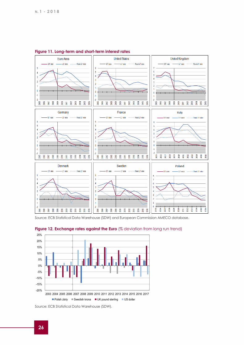
Monetary policy during the crisis has gradually softened as economic conditions deterio-
rated. This development is not fully reflected in the levels of real long-term interest rates
shown in Figure 11. In fact, when the room for negative short-run rates is constrained, other
unconventional measures had to supplement nominal long-term rate cuts. In a liquidity
trap, when the nominal short-run interest rate approaches the zero-lower-bound (in Figure
11 this is summarized by the grey areas indicating when the rate are below 1%), the effec-
tiveness of monetary policy sharply declines. In this case, the central bank can control nei-
ther the dynamic of the long-term interest rate nor inflation and runs the risk of de-anchor-
ing inflation expectations from the 2% target.
In most of the advanced economies, central banks continue to exert some control over
inflation, mostly by relying on forward guidance, namely the promise to keep the short-term
nominal rate to very low values for longer than necessary. They are thereby generating
inflation expectations at longer-term horizons. However, they have also attempted to cut
long-term interest rates by means of unconventional monetary policy (see Box 3). However,
while these policies were initially very effective in deeply troubled financial markets, they
have lost their power over the real long-term rate during the last few years. In 2015, real
long-term interest rates increased and eventually turned positive even though nominal
rates fell, because the inflation rate became negative in most countries. Nowadays, only
Germany and Sweden are facing negative real interest rates. In Germany, this phenome-
non is mostly attributable to very low (zero) long-term nominal interest rates coupled with
rising prices, while in Sweden it is a consequence of the ultra-loose monetary policy driving
the nominal short-term rates into negative territories as well. In Eastern European countries
with local currency, all interest rates were generally higher than in the Euro Area.
Outside the Euro Area most of the difference in the long-term interest rates is reflected in
the exchange rates dynamic, reported in Figure 12. For instance, after the Brexit vote (2016-
2017), sterling strongly depreciated against the Euro, and real interest rates in the UK en-
tered negative territories, although short-term interest rates were kept constant, or even
increased in the later quarters of 2017. However, within the European Monetary Union, the
divergence in the real long-term interest rates’ dynamic observed in the last years might
be attributable to country-specific policy, and in particular to heterogeneous fiscal stance.
N. 1 - 2 0 1 8
26
Figure 11. Long-term and short-term interest rates
Source: ECB Statistical Data Warehouse (SDW) and European Commission AMECO database.
Figure 12. Exchange rates against the Euro (% deviation from long run trend)
Source: ECB Statistical Data Warehouse (SDW).
-20%
-15%
-10%
-5%
0%
5%
10%
15%
20%
25%
2003 2004 2005 2006 2007 2008 2009 2010 2011 2012 2013 2014 2015 2016 2017
Polish zloty Swedish krona UK pound sterling US dollar
R A P P O R T O C E R
27 27
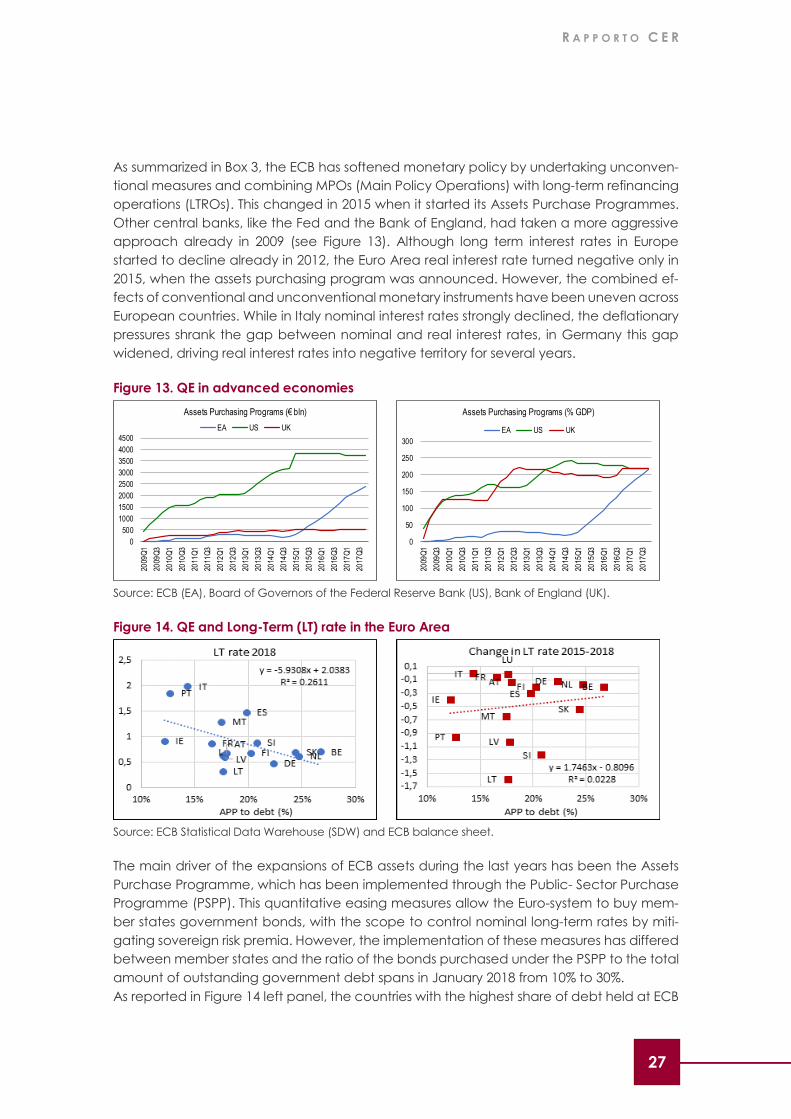
As summarized in Box 3, the ECB has softened monetary policy by undertaking unconven-
tional measures and combining MPOs (Main Policy Operations) with long-term refinancing
operations (LTROs). This changed in 2015 when it started its Assets Purchase Programmes.
Other central banks, like the Fed and the Bank of England, had taken a more aggressive
approach already in 2009 (see Figure 13). Although long term interest rates in Europe
started to decline already in 2012, the Euro Area real interest rate turned negative only in
2015, when the assets purchasing program was announced. However, the combined ef-
fects of conventional and unconventional monetary instruments have been uneven across
European countries. While in Italy nominal interest rates strongly declined, the deflationary
pressures shrank the gap between nominal and real interest rates, in Germany this gap
widened, driving real interest rates into negative territory for several years.
Figure 13. QE in advanced economies
Source: ECB (EA), Board of Governors of the Federal Reserve Bank (US), Bank of England (UK).
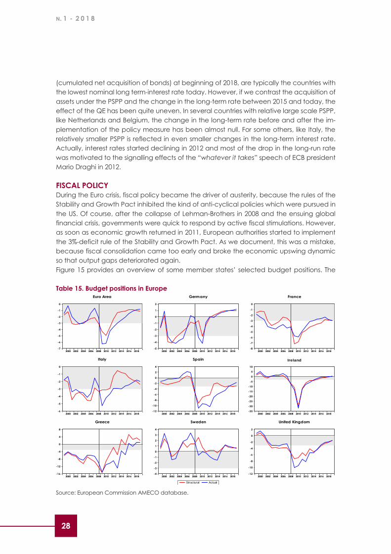
Figure 14. QE and Long-Term (LT) rate in the Euro Area
Source: ECB Statistical Data Warehouse (SDW) and ECB balance sheet.
The main driver of the expansions of ECB assets during the last years has been the Assets
Purchase Programme, which has been implemented through the Public- Sector Purchase
Programme (PSPP). This quantitative easing measures allow the Euro-system to buy mem-
ber states government bonds, with the scope to control nominal long-term rates by miti-
gating sovereign risk premia. However, the implementation of these measures has differed
between member states and the ratio of the bonds purchased under the PSPP to the total
amount of outstanding government debt spans in January 2018 from 10% to 30%.
As reported in Figure 14 left panel, the countries with the highest share of debt held at ECB
0
500
1000
1500
2000
2500
3000
3500
4000
4500
2009
Q1
2009
Q3
2010
Q1
2010
Q3
2011
Q1
2011
Q3
2012
Q1
2012
Q3
2013
Q1
2013
Q3
2014
Q1
2014
Q3
2015
Q1
2015
Q3
2016
Q1
2016
Q3
2017
Q1
2017
Q3
Assets Purchasing Programs (€ bln)
EA US UK
0
50
100
150
200
250
300
2009
Q1
2009
Q3
2010
Q1
2010
Q3
2011
Q1
2011
Q3
2012
Q1
2012
Q3
2013
Q1
2013
Q3
2014
Q1
2014
Q3
2015
Q1
2015
Q3
2016
Q1
2016
Q3
2017
Q1
2017
Q3
Assets Purchasing Programs (% GDP)
EA US UK
N. 1 - 2 0 1 8
28
(cumulated net acquisition of bonds) at beginning of 2018, are typically the countries with
the lowest nominal long term-interest rate today. However, if we contrast the acquisition of
assets under the PSPP and the change in the long-term rate between 2015 and today, the
effect of the QE has been quite uneven. In several countries with relative large scale PSPP,
like Netherlands and Belgium, the change in the long-term rate before and after the im-
plementation of the policy measure has been almost null. For some others, like Italy, the
relatively smaller PSPP is reflected in even smaller changes in the long-term interest rate.
Actually, interest rates started declining in 2012 and most of the drop in the long-run rate
was motivated to the signalling effects of the “whatever it takes” speech of ECB president
Mario Draghi in 2012.
FISCAL POLICY
During the Euro crisis, fiscal policy became the driver of austerity, because the rules of the
Stability and Growth Pact inhibited the kind of anti-cyclical policies which were pursued in
the US. Of course, after the collapse of Lehman-Brothers in 2008 and the ensuing global
financial crisis, governments were quick to respond by active fiscal stimulations. However,
as soon as economic growth returned in 2011, European authorities started to implement
the 3%-deficit rule of the Stability and Growth Pact. As we document, this was a mistake,
because fiscal consolidation came too early and broke the economic upswing dynamic
so that output gaps deteriorated again.
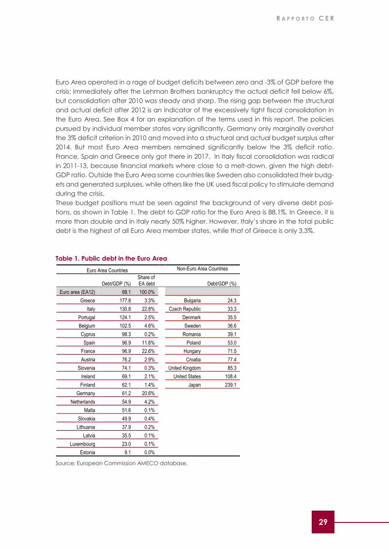
Figure 15 provides an overview of some member states’ selected budget positions. The
Table 15. Budget positions in Europe
Source: European Commission AMECO database.
-7
-6
-5
-4
-3
-2
-1
0
2000 2002 2004 2006 2008 2010 2012 2014 2016 2018
Euro Area
-5
-4
-3
-2
-1
0
1
2
2000 2002 2004 2006 2008 2010 2012 2014 2016 2018
Germany
-8
-7
-6
-5
-4
-3
-2
-1
0
2000 2002 2004 2006 2008 2010 2012 2014 2016 2018
France
-6
-5
-4
-3
-2
-1
0
2000 2002 2004 2006 2008 2010 2012 2014 2016 2018
Italy
-12
-10
-8
-6
-4
-2
0
2
4
2000 2002 2004 2006 2008 2010 2012 2014 2016 2018
Spain
-35
-30
-25
-20
-15
-10
-5
0
5
10
2000 2002 2004 2006 2008 2010 2012 2014 2016 2018
Ireland
-16
-12
-8
-4
0
4
8
2000 2002 2004 2006 2008 2010 2012 2014 2016 2018
Greece
-4
-3
-2
-1
0
1
2
3
4
2000 2002 2004 2006 2008 2010 2012 2014 2016 2018
Structural Actual
Sweden
-12
-10
-8
-6
-4
-2
0
2
2000 2002 2004 2006 2008 2010 2012 2014 2016 2018
United Kingdom
R A P P O R T O C E R
29 29
Euro Area operated in a rage of budget deficits between zero and -3% of GDP before the
crisis; immediately after the Lehman Brothers bankruptcy the actual deficit fell below 6%,
but consolidation after 2010 was steady and sharp. The rising gap between the structural
and actual deficit after 2012 is an indicator of the excessively tight fiscal consolidation in
the Euro Area. See Box 4 for an explanation of the terms used in this report. The policies
pursued by individual member states vary significantly. Germany only marginally overshot
the 3% deficit criterion in 2010 and moved into a structural and actual budget surplus after
2014. But most Euro Area members remained significantly below the 3% deficit ratio.
France, Spain and Greece only got there in 2017. In Italy fiscal consolidation was radical
in 2011-13, because financial markets where close to a melt-down, given the high debt-
GDP ratio. Outside the Euro Area some countries like Sweden also consolidated their budg-
ets and generated surpluses, while others like the UK used fiscal policy to stimulate demand
during the crisis.
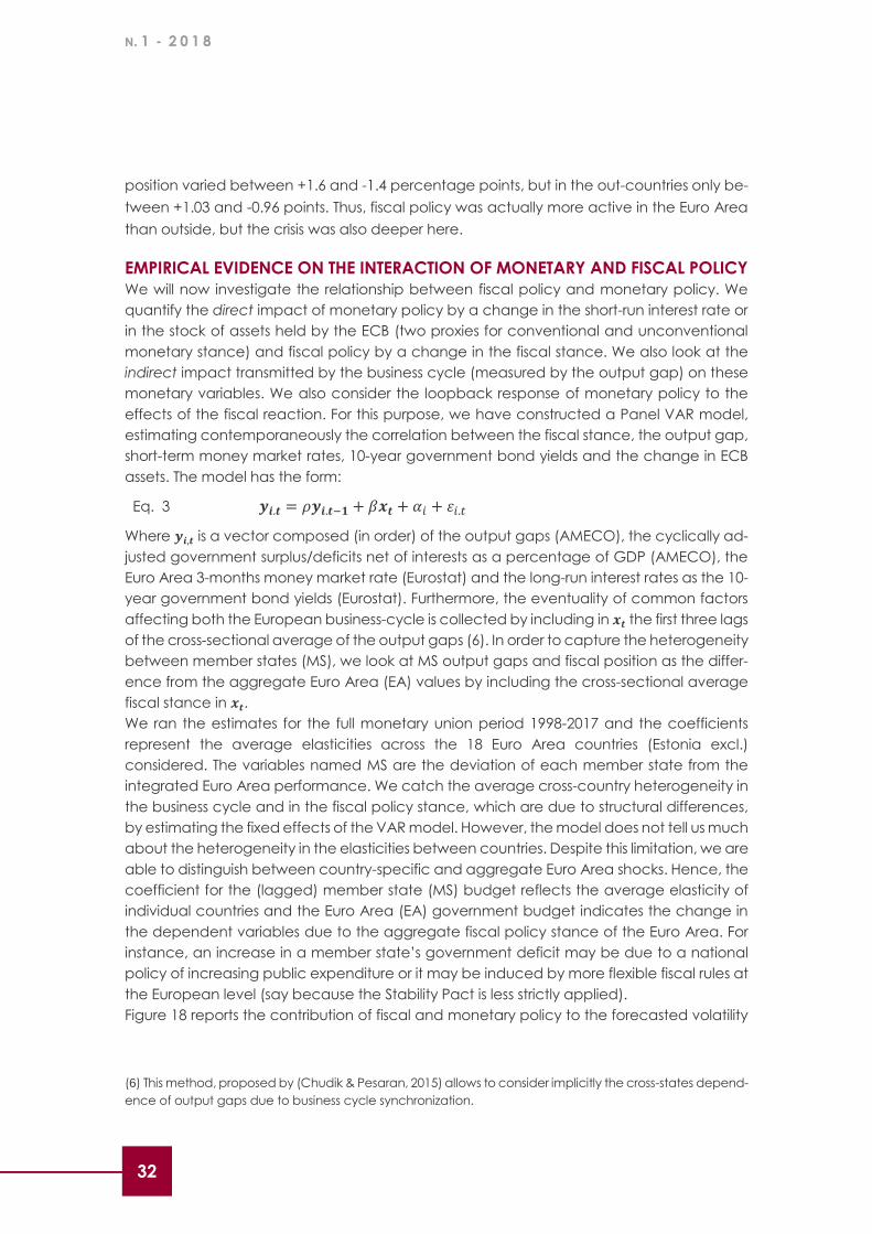
These budget positions must be seen against the background of very diverse debt posi-
tions, as shown in Table 1. The debt to GDP ratio for the Euro Area is 88.1%. In Greece, it is
more than double and in Italy nearly 50% higher. However, Italy’s share in the total public
debt is the highest of all Euro Area member states, while that of Greece is only 3.3%.
Table 1. Public debt in the Euro Area
Source: European Commission AMECO database.
Euro Area Countries Non-Euro Area Countries
Debt/GDP (%) Share of EA debt
Debt/GDP (%)
Euro area (EA12) 88.1 100.0%
Greece 177.8 3.3% Bulgaria 24.3
Italy 130.8 22.8% Czech Republic 33.3
Portugal 124.1 2.5% Denmark 35.5
Belgium 102.5 4.6% Sweden 36.6
Cyprus 98.3 0.2% Romania 39.1
Spain 96.9 11.6% Poland 53.0
France 96.9 22.6% Hungary 71.5
Austria 76.2 2.9% Croatia 77.4
Slovenia 74.1 0.3% United Kingdom 85.3
Ireland 69.1 2.1% United States 108.4
Finland 62.1 1.4% Japan 239.1
Germany 61.2 20.6%
Netherlands 54.9 4.2%
Malta 51.6 0.1%
Slovakia 49.9 0.4%
Lithuania 37.9 0.2%
Latvia 35.5 0.1%
Luxembourg 23.0 0.1%
Estonia 9.1 0.0%

N. 1 - 2 0 1 8
30
Figure 16. Annual Standard Deviation of budget positions
Source: European Commission AMECO database and CER computations.
Despite the constraining fiscal rules, budget positions have been more volatile in the Euro
Area during the crisis then outside. Figure 16 shows that the cross-country standard devia-
tion of actual budget deficits within the EMU has been significantly higher between 2008
and 2014 than in the Non-Euro Area countries. However, the standard deviation of the
structural deficits has been in excess of the Non-Euro Area only immediately after the Leh-
man-Brothers bankruptcy and in the depth of the Euro-crisis.
The excessively tight fiscal stance, especially between 2011 and 2014, is also documented
by Figure 17. The premature tightening is clear from the movements of the fiscal stance
Figure 17. Euro Area fiscal stance
1
2
3
4
5
6
7
2000
2002
2004
2006
2008
2010
2012
2014
2016
2018
Le
hm
an
De
fau
lt
Structural Budget Position
1
2
3
4
5
6
7
2000
2002
2004
2006
2008
2010
2012
2014
2016
2018
Euro Area St. Dev . Non-Euro Area St. Dev .
Le
hm
an
De
fau
lt
Actual Budget Position

R A P P O R T O C E R
31 31
cont. Figure 17. Euro Area fiscal stance
Source: European Commission AMECO database and CER computations.
between 2009 and 2011. Only in 2015-16 did the Euro Area take a weak anti-cyclical and
stimulating position that is now turning into pro-cyclical loosening. This was different in Non-
Euro Area member states, which generally followed anti-cyclical policies.
The fiscal policy stance is measured by the variation of the cyclically adjusted structural
deficit net of interest rates. The Euro Area’s restrictive policy stance reflected the require-
ments in Germany, where – take in isolation - the relatively expansive boom would have
justified anti-cyclical tightening in 2011 and in 2012 (see Figure 12 and Figure 17), but it did
not take into consideration the more adverse conditions in some of the other Euro Area
economies. The alternating policy mix in Greece between tightening and loosening re-
flects the confused approach to the sovereign debt crisis in Greece. It is, however, interest-
ing that the policy mix in the Non-Euro Area countries was generally more anti-cyclical and
the fiscal policy stance was more stable: changes in the cyclically adjusted primary budget
20072008
20092010
2011
2012
2013
2014
2015
2016
2017
2018
2019
y = -0.1622x - 0.3699R² = 0.0778
-6
-4
-2
0
2
4
6
8
10
-20 -15 -10 -5 0 5 10
Tit
le
Title
Greece
anticyclical tightening
anticyclical losening
procyclical tightening
procyclical losening
N. 1 - 2 0 1 8
32
position varied between +1.6 and -1.4 percentage points, but in the out-countries only be-
tween +1.03 and -0.96 points. Thus, fiscal policy was actually more active in the Euro Area
than outside, but the crisis was also deeper here.
EMPIRICAL EVIDENCE ON THE INTERACTION OF MONETARY AND FISCAL POLICY
We will now investigate the relationship between fiscal policy and monetary policy. We
quantify the direct impact of monetary policy by a change in the short-run interest rate or
in the stock of assets held by the ECB (two proxies for conventional and unconventional
monetary stance) and fiscal policy by a change in the fiscal stance. We also look at the
indirect impact transmitted by the business cycle (measured by the output gap) on these
monetary variables. We also consider the loopback response of monetary policy to the
effects of the fiscal reaction. For this purpose, we have constructed a Panel VAR model,
estimating contemporaneously the correlation between the fiscal stance, the output gap,
short-term money market rates, 10-year government bond yields and the change in ECB
assets. The model has the form:
Eq. 3 𝒚𝒊,𝒕 = 𝜌𝒚𝒊,𝒕−𝟏 + 𝛽𝒙𝒕 + 𝛼𝑖 + 𝜀𝑖,𝑡
Where 𝒚𝒊,𝒕 is a vector composed (in order) of the output gaps (AMECO), the cyclically ad-
justed government surplus/deficits net of interests as a percentage of GDP (AMECO), the
Euro Area 3-months money market rate (Eurostat) and the long-run interest rates as the 10-
year government bond yields (Eurostat). Furthermore, the eventuality of common factors
affecting both the European business-cycle is collected by including in 𝒙𝒕 the first three lags
of the cross-sectional average of the output gaps (6). In order to capture the heterogeneity
between member states (MS), we look at MS output gaps and fiscal position as the differ-
ence from the aggregate Euro Area (EA) values by including the cross-sectional average
fiscal stance in 𝒙𝒕.
We ran the estimates for the full monetary union period 1998-2017 and the coefficients
represent the average elasticities across the 18 Euro Area countries (Estonia excl.)
considered. The variables named MS are the deviation of each member state from the
integrated Euro Area performance. We catch the average cross-country heterogeneity in
the business cycle and in the fiscal policy stance, which are due to structural differences,
by estimating the fixed effects of the VAR model. However, the model does not tell us much
about the heterogeneity in the elasticities between countries. Despite this limitation, we are
able to distinguish between country-specific and aggregate Euro Area shocks. Hence, the
coefficient for the (lagged) member state (MS) budget reflects the average elasticity of
individual countries and the Euro Area (EA) government budget indicates the change in
the dependent variables due to the aggregate fiscal policy stance of the Euro Area. For
instance, an increase in a member state’s government deficit may be due to a national
policy of increasing public expenditure or it may be induced by more flexible fiscal rules at
the European level (say because the Stability Pact is less strictly applied).
Figure 18 reports the contribution of fiscal and monetary policy to the forecasted volatility
(6) This method, proposed by (Chudik & Pesaran, 2015) allows to consider implicitly the cross-states depend-
ence of output gaps due to business cycle synchronization.

R A P P O R T O C E R
33 33
of selected variables; Figure 19 shows the Impulse Response Functions (IRF) after a negative
shock to the short term interest rate or after an improvement in the fiscal stance. Those
results jointly show how the output gap, fiscal policy and monetary policy (i.e. short and
long term interst rates) respond to the various shocks.
Figure 18. Fiscal and monetary policy contribution to the volatility of selected variables
Source: ECB Statistical Data Warehouse (SDW), EC AMECO database and CER computations.
Figure 19. Panel VAR on the monetary and fiscal policy mix in the Euro Area
IRFs to a shock to either the short-term rate (-1 p.p.) or to the government surplus-to-GDP (+1 p.p.)
Source: European Commission AMECO database and CER computations.
0%
5%
10%
15%
20%
25%
30%
35%
40%
Output
Gap
ECB
assets
Long-term
rate
Short-term
rate
Gov.
Budget
Output
Gap
ECB
assets
Long-term
rate
Short-term
rate
Gov.
Budget
2-year 5-year
FE
VD
Response Varibale and time horizon
Output Gap ECB assets Long-term rate Short-term rate Gov. Budget
0,00
0,10
0,20
0,30
0,40
0,50
0,60
0,70
0,80
0,90
1,00
0 1 2 3 4 5
Output Gap
Short-Term Interest Rate Government Surplus/Deficit
-1,20
-1,00
-0,80
-0,60
-0,40
-0,20
0,00
0,20
0,40
0 1 2 3 4 5
Short-Term Interest Rate
Short-Term Interest Rate Government Surplus/Deficit
-0,35
-0,30
-0,25
-0,20
-0,15
-0,10
-0,05
0,00
0 1 2 3 4 5
Long-Term Interest Rate
Short-Term Interest Rate Government Surplus/Deficit
-0,20
0,00
0,20
0,40
0,60
0,80
1,00
1,20
0 1 2 3 4 5
Government Surplus/Deficit
Short-Term Interest Rate Government Surplus/Deficit

N. 1 - 2 0 1 8
34
We start with the determinants of the forecasted volatility of selected variables in Figure 18.
The output gap is not explained by the government budget position, nor is the government
budget volatility affected by output gap volatility in the medium run. We interpret this as a
sign for the inconsistent fiscal policy stances shown in Figure 17. Hence, better policy
coordination would improve the economic performance of the Euro Area. Furthermore,
monetary policy is highly significant. The contribution to output gap volatility by short-term
interest rate changes, which are controlled by the ECB, is larger than for long-term rates;
the impact by unconventional monetary policy measures, which have expanded the ECB
balance sheet, is even stronger. This confirms the excessive burden for monetary policy in
the European policy mix.
Furthermore, we turn to the analysis of the dynamic response to either a monetary or a
fiscal policy shock. We start by looking at the impact on the output gap in the top-left panel
of Figure 19. First of all, we observe that output gaps respond quickly to monetary policy,
but are rather persistent in the long run. The response to a fiscal policy shock is slow and
weak. Another striking result, although not reported here, is that it is positively correlated
with the aggregate output gap of the Euro Area. This clearly means that by improving the
policy mix for the Euro Area as a whole, the economic conditions in each member state
will improve. This is an important argument in favour of better macroeconomic policy
coordination at the European level.
Second, this latter result is confirmed by the dynamics of the member states fiscal stance
after a monetary shock, because fiscal policy does not respond to monetary policy,
supporting the view that fiscal stance is an independent and autonomous decision.
Third, monetary policy (proxied by short-term interest rate) responds weakly to country-
specific conditions, as shown in Figure 19, but strongly to the Euro Area aggregate fiscal
stance. Hence, monetary policy does not respond to fiscal policy in member states, but in
fact, the ECB lowers short-term rates exclusively in response to fiscal consolidation in the
aggregate Euro Area stance while increases them when the output gap turns positive and
risks generating inflation. This is in line with our discussion of the policy mix (see Box 2).
Finally, we found that monetary policy does affect real long run interest rate in Figure 18 in
the short run, but in the medium run the dynamics also depends on government budget
positions. A similar conclusion can be drawn from the IRFs of Figure 19. In fact, from the
second year onwards there is no difference between the IRFs after an expansionary
monetary or a contractionary fiscal policy shock. This highlights that the effectiveness of
monetary policy in shaping the dynamic of the long-term rate, is highly dependent on the
fiscal policy stance.
After a cut in the short-term interest rate, the government balance deteriorates (weakly),
causing an increase in the sovereign spread, hence in the long-term interest rate, which
bounds back towards the equilibrium. Therefore, since fiscal policies are highly
heterogenous among the countries, the effectiveness of monetary policy in stimulating the
economy is highly uneven across countries. As previously shown in Figure 10, in the last years
the correlation between fiscal stance and long-term rates has turned from clearly negative
trade-off to a highly non-linear relation. It follows that the fiscal expansions before the crisis
were counterproductive because they increased the long-term rates, while today with
higher fiscal policy heterogeneity, monetary policy might have become more supportive.

R A P P O R T O C E R
35 35
In the decade since 2008, monetary policy was constrained by the zero-lower-bound of
nominal interest rates, but by using a combination of long run refinancing operations and
quantitative easing, the ECB was able to exert some direct control on the long-term rate,
thereby increasing its effectiveness. We have run estimations for different measures of ECB
balance sheets for the unconventional monetary policy stance over the period 2009-2017:
Long Term Refinancing Operations (LTRO, TLTRO, etc.), and total securities and government
lending, or the sum of the two. In Figure 20 we show the responses of the output gap, the
money market rate, government stance and 10-year yield to an increase of 1 p.p. of GDP
in either the securities held for policy purposes (blue line) or in the overall assets purchased
for unconventional monetary policy (LTRO plus APP). We do not report the responses after
an increase in the LTRO’s assets because those policies had heterogenous effects over the
period considered, since target operations were much more effective than initial LTRO. The
monetary-fiscal policy interaction was even stronger during those years than before the
crisis, because after an increase in ECB assets for monetary purposes, either just in the form
of securities or combined with Long-Term Refinancing Operations, short-term interest rates
dropped, while in the first-year long-term interest rates rose because the government bal-
ances deteriorated, pushing up interest spreads. However, and this is important, the large
increase in the long-term interest rate is the driver of the small widening in the output gap.
Therefore, most of the relative ineffectiveness of quantitative easing measures is attributa-
ble to fiscal policy moral hazard.
Figure 20. Panel VAR on the monetary and fiscal policy mix in the Euro Area
IRFs to a shock to the ECB assets (+ 1mln)
Source: European Commission AMECO database and CER computations.
-1,4
-1,2
-1,0
-0,8
-0,6
-0,4
-0,2
0,0
0 1 2 3 4 5
Output Gap
ECB Assets EBC Securities
-1,8
-1,6
-1,4
-1,2
-1,0
-0,8
-0,6
-0,4
-0,2
0,0
0 1 2 3 4 5
Short-Term Interest Rate
ECB Assets EBC Securities
-0,5
-0,4
-0,3
-0,2
-0,1
0,0
0,1
0,2
0,3
0 1 2 3 4 5
Long-Term Interest Rate
ECB Assets EBC Securities
-0,8
-0,7
-0,6
-0,5
-0,4
-0,3
-0,2
-0,1
0,0
0 1 2 3 4 5
Government Surplus/Deficit
ECB assets EBC Securities

N. 1 - 2 0 1 8
36
BOX 2. FISCAL-MONETARY POLICY MIX IN THEORY
The relation between stability, fiscal and monetary policy, and democracy can be described by a
set of four simple equations:
Eq. 4 Stability condition: 𝑦 – 𝑦∗ = 𝜑0 − 𝜑1𝑟 − 𝜑2𝑠
Eq. 5 Monetary policy rule: 𝑟 = 𝑟∗ + 𝑓(𝜋 − 𝜋∗)
Eq. 6 Efficiency frontier: 𝑟∗ = 𝜑0
𝜑1−
𝜑2
𝜑1𝑠
Eq. 7 Welfare function: 𝑈 = 𝑟𝛼𝑠1−𝛼
Equation 3 gives the stability condition whereby the output gap is a function of interest rates are and
the primary surplus of the government. Equation 4 gives the monetary public policy rule, whereby the
central bank sets the interest rate as a mark-up over the long run natural rate at which price stability
is ensured. The efficiency frontier (Eq. 5) will then establish the trade-off between equilibrium interest
rates and fiscal positions. Finally, equation 6 is the welfare function by which the utility of a society is
determined by the relative weight given to interest rates or fiscal policy. Democracy is modelled as
the shifting of these consensual weights through elections.
Figure B2.1. Policy Mix
The relation between monetary and fiscal policy is expressed by Figure B2.1, which is derived from
the equations above. It shows the monetary proxy r (for real interest rate) on the vertical axis and the
fiscal position (cyclically adjusted primary surplus, s) on the horizontal axis. On the right of the vertical
zero-line, the budget is in surplus, to the left it is in deficit. The downward sloping line, which goes
through the points R and E is the efficiency line that models the trade-off between higher interest
rates and a negative budget balance versus lower interest rates and a budget surplus. Any point on
the efficiency line is efficient in the sense that output gaps are zero. This means that the efficiency line
represents cyclically adjusted budget positions. Above the efficiency line the policy mix is too restric-
tive and therefore causing depressions, below the efficiency line, it is too lose creating inflation.
Hence, the efficiency line is the locus of multiple equilibria. In order to choose an optimal policy- mix,
we need to add the welfare function. At point R the deficit is relatively high and so are interest rates;
at point E the budget is balanced, and interest rates are low.

R A P P O R T O C E R
37 37
All points above the efficiency line reflect an excessively tight policy mix, so that negative output
gaps are on the right side above the equilibrium, while points below this line signal a stimulating policy
mix. An excessively tight policy mix can be adjusted by easier monetary policy (lower interest rates)
or by a looser fiscal policy stance (higher deficits).
The so-called automatic stabilizers of fiscal policy imply that the cyclically adjusted “structural” deficit
reflects the position on the efficiency line, while actual deficits vary during the business cycle. How-
ever, fiscal policy requires taking a pro-active stance with respect to the interaction between fiscal
and monetary policy.

N. 1 - 2 0 1 8
38
BOX 3. THE ECB UNCONVENTIONAL MONETARY STANCE
The relation between stability, fiscal and monetary policy, and democracy can be described by a
set of four simple equations:
Phases of The Crisis Problems Remedies
I. Liquidity crisis
after Lehman
bankruptcy
2008 - 2010
Excessive lending in boom
• Uncertainty about scale of
exposure to subprime
products
• Sudden stop of money
market funding
• Rush to cash
• Lower main refinancing rate
to 1%
• Longer duration for liquidity
provisions
• Enlarged ECB balance sheet
II. Sovereign
Debt Crisis
2011-2014
Bank-sovereign nexus
• Risk of bank exposure to
government defaults
• Risk of assets fire sales by
banks
• Disruption of monetary
transmission channel
• Sovereign spread expressing
redenomination risk, distorted
asset prices and credit
conditions
• Lengthening maturity
operations
• Expanding range of eligible
collateral
• Outright monetary
transactions
III. Return to
Equilibrium
2014-2018
Balance sheet recession
• Corporate deleveraging led
to reduce lending (credit
crunch)
• Risk of deflation due to
savings-investment
imbalances
• Very negative equilibrium
interest rates
• November 2013: rate cuts to
0.25%
• Introduced forward
guidance
• Negative interest rates on
ECB deposit facility
• Flattening short end of yield
curve
• Asset Purchase Program
(APP): covered bonds, asset-
backed securities, sovereign
and corporate bonds
• Target long term refinancing
operations (TLTRO)

R A P P O R T O C E R
39 39
BOX 4. GLOSSARY FOR FISCAL POLICY TERMS
The budget position of general government is the difference between government revenue and ex-
penditure (T-G). A negative position is it deficit, a positive position is a surplus. Surpluses are also called
net lending, or net government savings; a deficit is public sector net borrowing. The total budget
position is the sum of the structural and cyclical component of the budget.
The cyclical component of the budget position reflects short-term shocks to the income or expendi-
ture of the government. Because a negative income shock which reduces tax income and forces
the government to borrow, the cyclical component of the budget position is also often called auto-
matic stabilizer.
◼ This structural or cyclically adjusted budget position indicates the underlying balance between
long-term government revenues and expenditure, while removing factors that are attributable to
shocks or the business cycle.
◼ The primary budget position is the difference of revenue minus expenditure net of interest charges.
It indicates the discretionary room for governments to adjust their net spending.
◼ The fiscal stance is the change in the cyclically adjusted primary budget position which represents
a change in policy orientation
The methodological problems of measuring cyclical and structural budget positions are substantial.
For details and discussion see:
https://www.bundesbank.de/Redaktion/EN/Downloads/Publications/Monthly_Report_Arti-
cles/1997/1997_04_budget_deficits.pdf?__blob=publicationFile

R A P P O R T O C E R
41 41
European Fiscal Union
Economic theory assigns three distinct functions to public finance: the stabilisation function,
the distribution function, and the allocation function. European Fiscal Union is about the
stabilisation of macroeconomic aggregates by an appropriate policy mix. Because effec-
tive demand is monetary purchasing power, the management of macroeconomic stabili-
sation must be centralized at the level of the monetary union. A transfer union is dealing
with the redistribution of income between rich and poor regions and income groups. Such
re-distribution requires a high degree of solidarity, which is often assumed to be absent in
the European Union. However, the budget of the European Union is already a small instru-
ment for making such transfers. Finally, the allocation function involves principles of fiscal
federalism, i.e. the allocation of responsibilities for making decisions on the provision of pub-
lic goods. When President Macron spoke of “the great challenges of our times, such as
defence and security, great migrations, development, climate change, the digital revolu-
tion and regulation of a globalized economy”, he effectively described European public
goods, which are at the moment allocated inefficiently by national governments and not
by a European authority.
In this chapter we deal with the flow of funds in a European fiscal union. In the next chapter
we will look at the European budget and conclude discussing some issues of fiscal federalism.
FISCAL POLICY COORDINATION IN THE EURO AREA
During the Euro crisis it became popular to ascribe the debt problems of the Southern coun-
tries by the accumulation of current account deficits. The logic behind this argument is that
excessive borrowing by governments (the sovereign debt crisis in Greece) or by private
investors (the real estate crisis in Spain and Ireland) had led to unsustainable “foreign” debt
levels. According to national income identities, these imbalances are reflected in current
account positions (see Eq. 8 below), and they add up to the external debt position of a
country. The European Commission even built its new Macroeconomic Imbalance Proce-
dure on this reasoning. However, the focus on current account deficits is misleading: first,
such deficits mean that the country is running out of foreign exchange and will ultimately
be forced to depreciate its currency. However, within a currency union there are no for-
eign exchange reserves and a country cannot run out of money. The money to make a
payment in another member state comes from the ECB and is distributed through the
banking system. The ECB steers money supply in line with its primary objective of preserving
price stability in the Euro Area as a whole, but whether debt is sustainable or not depends
on credit status of the debtor and not on the debtor’s nationality. Hence, member states
in the monetary union are not “foreign” countries, but regions of the currency union. Nev-
ertheless, within the Eurozone context debt financed fiscal expansions increase trade def-
icits (7), and this implies significant spill-overs to the private sector of other member states,
as we will see below.
(7) See (Beetsma, et al., 2008).
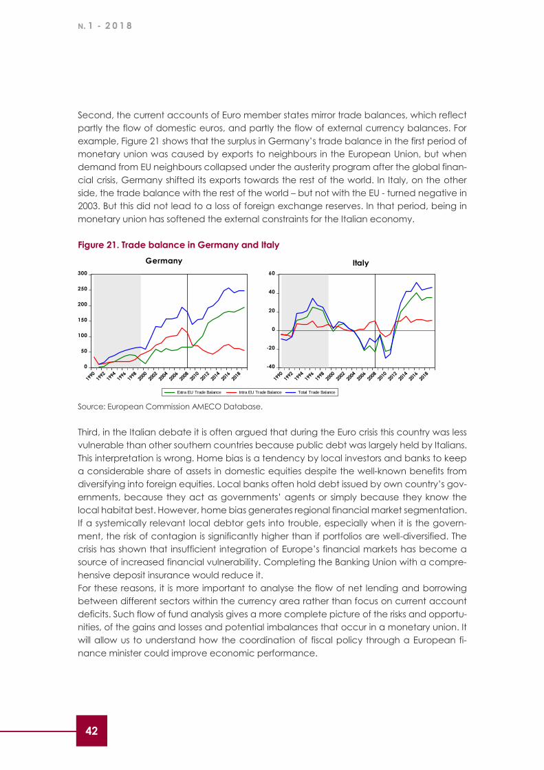
N. 1 - 2 0 1 8
42
Second, the current accounts of Euro member states mirror trade balances, which reflect
partly the flow of domestic euros, and partly the flow of external currency balances. For
example, Figure 21 shows that the surplus in Germany’s trade balance in the first period of
monetary union was caused by exports to neighbours in the European Union, but when
demand from EU neighbours collapsed under the austerity program after the global finan-
cial crisis, Germany shifted its exports towards the rest of the world. In Italy, on the other
side, the trade balance with the rest of the world – but not with the EU - turned negative in
2003. But this did not lead to a loss of foreign exchange reserves. In that period, being in
monetary union has softened the external constraints for the Italian economy.
Figure 21. Trade balance in Germany and Italy
Source: European Commission AMECO Database.
Third, in the Italian debate it is often argued that during the Euro crisis this country was less
vulnerable than other southern countries because public debt was largely held by Italians.
This interpretation is wrong. Home bias is a tendency by local investors and banks to keep
a considerable share of assets in domestic equities despite the well-known benefits from
diversifying into foreign equities. Local banks often hold debt issued by own country’s gov-
ernments, because they act as governments’ agents or simply because they know the
local habitat best. However, home bias generates regional financial market segmentation.
If a systemically relevant local debtor gets into trouble, especially when it is the govern-
ment, the risk of contagion is significantly higher than if portfolios are well-diversified. The
crisis has shown that insufficient integration of Europe’s financial markets has become a
source of increased financial vulnerability. Completing the Banking Union with a compre-
hensive deposit insurance would reduce it.
For these reasons, it is more important to analyse the flow of net lending and borrowing
between different sectors within the currency area rather than focus on current account
deficits. Such flow of fund analysis gives a more complete picture of the risks and opportu-
nities, of the gains and losses and potential imbalances that occur in a monetary union. It
will allow us to understand how the coordination of fiscal policy through a European fi-
nance minister could improve economic performance.
0
50
100
150
200
250
300
1990
1992
1994
1996
1998
2000
2002
2004
2006
2008
2010
2012
2014
2016
2018
-40
-20
0
20
40
60
1990
1992
1994
1996
1998
2000
2002
2004
2006
2008
2010
2012
2014
2016
2018
Extra EU Trade Balance Intra EU Trade Balance Total Trade Balance
Germany Italy

R A P P O R T O C E R
43 43
THE FLOW OF FUNDS ANALYSIS
In a monetary economy, goods are not exchanged but sold for money. This means for
every transfer of goods and services there is a counter-movement in the form of money
flows. The expenditure of the buyer is the income of the seller. The asset of the lender is the
liability of the borrower. Spending in excess of income requires borrowing financial surpluses
from other sources. A financial surplus is also called net lending, and a financial deficit net
borrowing (8). A financial surplus can be used either to build up financial assets or to repay
debt and deleverage balance sheets. Deleveraging may be desirable to reduce financial
risks, but in that case the money is not spent on goods and services so that it will lead to
recessions.
To analyse the flow of payments in the Euro Area, we distinguish between four institutional
sectors: households save and lend their money to corporations who borrow to invest. Gov-
ernments either save by running budget surpluses or borrow to finance deficits. Finally,
households, corporations and governments can borrow from or lend to the rest of the
world. The sum of all these net borrowings and lendings is always zero.
Flow of funds analysis reveals the flows of payments between economic sectors and re-
gions. We will first discuss the sectoral relations and then the regional implications. In a text
book setting, households save and lend to the corporate sector which invests these funds
and thereby generates income, while government budgets and the current account are
in balance. In reality, this is rarely the case. If the balance between household net savings
and the corporate sector’s net borrowing is positive (S – I > 0), this net lending of the private
sector must be absorbed by government net borrowing (T – G < 0) or by the rest of the
world (CA > 0), otherwise, a recession will occur. But if the private sector net balance is
negative (S – I < 0), the financing gap of the private sector must be closed by borrowing
from banks, the government (i.e. net tax reductions) or from abroad. If these excess savings
are not absorbed by borrowing, they become idle money and cause aggregate income
to shrink, thereby causing unemployment. On the other hand, if the demand for funds ex-
ceeds the sum of savings by households and by the government, foreign investors or banks
will have to close the gap (9). Yet, bank lending creates money supply (10), and if this
money creation is excessive it will create inflation. Hence, what determines the perfor-
mance of a monetary economy is the flow of net lending and net borrowing between
different sectors in the economy.
National income identities help us to identify the net flow of borrowing and lending. They
tell us that the current account balance (CA = X - M) is the sum of the net savings-invest-
ment balance (S-I) of the private sector and the government budget position (T-G):
Eq. 8 CA = (S – I) + (T- G)
(8) For simplicity we have aggregated Monetary and Financial Institutions and Non-financial corporations.
(9) The sum of private and public-sector saving is also called national saving:
Snat = S + (T-G) = (Y-T-C) + (T-G) = Y-(C+G)
(10) “Loans make deposits” is the formula by which modern monetary theory explains money creations.
See (McLeay, et al., 2014). In the old days, economists spoke about the government using the printing press.

N. 1 - 2 0 1 8
44
S stands here for household savings, I for investment, T for tax income, and G for govern-
ment spending. In a closed or balanced economy (CA = 0), national savings (i.e. the sum
of private household saving S and government saving (T-G) are always equal to invest-
ment). These are balance sheet identities, but the economic literature provides different
models for explaining the dynamics of net lending and borrowing between sectors and
the responses to fiscal policy impulses. We are particularly interested into the effect of fiscal
policy on the flow of funds within the monetary union.
A budget surplus (T > G) is government saving (net lending) and a budget deficit is net
public sector borrowing (see Box 4). Fiscal consolidation means the government lowers its
deficit or increases its surplus, which represents an increase in net government lending. A
fiscal expansion is the opposite. Standard macroeconomic theory focuses on the multiplier
effect of government budget positions on the private sector (11). However in monetary
union, the policy decisions by national governments and the reactions by the private sec-
tor have spillover effects into other member states, because if fiscal policy changes aggre-
gate demand in one country, consumers and investors from all countries will seek to exploit
the new opportunities (or avoid new risks). The spill-overs will then spill back into the original
member state, where it will affect government revenue and therefore the local fiscal
stance. Previous literature has already provided evidence of the large magnitude of those
spill-overs inside the Euro Area in terms of different measures of fiscal stance (revenues,
government consumption, debt-to-GDP, yield spread, etc.), as summarized in Box 5.
We distinguish five classical patterns for the interaction of fiscal policy with private sector
net lending.
1. In standard Keynesian models a fiscal consolidation (an increase in government sav-
ing) either will increase taxes, thereby lowering disposable income for consumption, or
will reduce public spending. Either way, the fiscal consolidation will depress consump-
tion and investment, so that private sector net lending (S-I) will increase. In this case
our estimated multiplier would be positive.
2. Crowding out occurs when the expansionary fiscal policy reduces investment, be-
cause the government’s demand for loanable funds pushes up interest rates. If the
productivity of private investment is higher than public spending, this will cause a slow-
down in economic growth. Crowding out is the limit for Keynesian policies, which
emerges when productive capacities are fully employed.
3. The opposite are so-called non-Keynesian effects when a fiscal consolidation reduces
the risk premium for unsustainable public debt and this stimulates investment and con-
sumption, so that a fiscal contraction will lead to an economic expansion. Here, the
fiscal multiplier is negative, as the lower deficit or higher budget surplus reduces the
risk premium for investors, so that the private surplus (S-I) shrinks. This is crowding in of
private investment by fiscal policy.
4. Ricardian Equivalence models argue that an increase in government savings trans-
lates one to one into a reduction in private savings, so that fiscal policy is neutral (an
(11) Frequently, the multiplier of fiscal policy is measured as the effect on GDP. We concentrate on the
saving or net lending in the private sector, which comes to the same. See (Giavazzi, et al., 1999) for a similar
approach.

R A P P O R T O C E R
45 45
increase in government savings generates a reduction in taxes, higher consumption
and investment and lower household savings). In this case, our estimated multiplier is
minus 1.
5. Finally, in the twin-deficit case, it is lending and borrowing from the rest of the world
that complement domestic funds. Hence, the current accounts are not necessarily
balanced, so that an increase in government savings (fiscal consolidation) will simul-
taneously decrease the current account deficit. However, this makes only sense if the
economy operates as in Keynesian models. In case of Ricardian Equivalence, there
should be no effect from fiscal policy to current accounts, and if public sector borrow-
ing crowds out private investment, the long-run effect would be zero, too. In the case
of non-Keynesian effects, a budget deficit reduction would even increase the current
account deficit.
So far, we have reasoned in terms of the two main institutional sectors (private and public)
of any economy. We will now add member states as geographical sectors of the Euro
Area. This renders the argument more complex but does not change the basic logic of
flows of funds. To show this logic while keeping things simple, we may assume that the Euro
Area as a whole has a balanced current account and is composed of two countries. We
can then decompose Eq. 9 into two sectors standing for region 1 and 2:
Eq. 9 CA= CA1 + CA2 = 0 => CA1 = - CA2
Eq. 10 (S1 – I1) + (T1- G1) = -(S2 – I2) - (T2- G2)
It is then obvious that the current account position, i.e. the flow of funds into one region, is
the mirror of the rest of the Euro area. If the savings in one region are insufficient to finance
local investment, savings from another region will have to provide the funds.
There are now two ways how this imbalance can be financed. First, in a properly function-
ing financial market (i.e. without home bias) the flow of lending and borrowing is uncon-
strained, so that household savings in one country will be lent to investors in other member
states – provided the risk-return conditions are attractive. For this reason, competitiveness,
as measured above, is a good indicator for where the flow of funds will go. Economic pol-
icies by national governments may improve these conditions, but if they fail and investment
is blocked by asymmetric investor expectations, it may be appropriate to unblock it at the
European level. This would be one of the functions of a European finance minister.
Second, it is often argued that the Euro Area does not function as a fully integrated cur-
rency union because it lacks fiscal transfers. A transfer union would imply that the budget
surplus of one government finances the deficit of another government:
Eq. 11 (T1- G1) = - (T2- G2) Transfer Union definition
Clearly, a transfer union is not a necessary requirement for transferring funds between
member states in monetary union, because the savings-investment balance in the private
sector can fulfil this function. In fact, in a monetary union with a single market and a fully
integrated banking union, the adjustment of shocks works primarily through the private sec-
tor channel and this explains the relative robustness of monetary unions, which fixed ex-

N. 1 - 2 0 1 8
46
change rate arrangements can never achieve. It is, however, true that the social conse-
quences of such adjustments can be harsh. In nation states fiscal policy serves as a redis-
tribution tool to cushion shocks, but in the European Union the use of fiscal policy for the
purpose of improving social welfare has not yet been accepted.
Nevertheless, fiscal policy in the European monetary union is not neutral, because the
changes of fiscal stances will generate spillover effects in neighbouring member states.
These effects will impact the balance of private net lending though changes in income,
consumption and investment, which spills back on neighbouring budget positions and ulti-
mately comes back to the original member state. Hence, even without a fiscal union, and
even without any form of fiscal coordination, national fiscal policies generate externalities
for all member states. These externalities are lower for countries outside the currency area,
because exchange rate adjustments inhibit the flow of funds.
How fiscal policy affects these different sectoral and regional flows of funds cannot be
decided on theoretical grounds, but an empirical matter. We have estimated the relevant
coefficients, as is common in the literature, in a global vector autoregressive model
(GVAR), which indicates the structure that holds the Euro Area together. Following
Dragomirescu-Gaina & Philippas (2015) we apply the GVAR estimator to a set of variables
composed of the net lending of the public and private sector, and we consider the
weighted trade flow variables as the main transmission channel, as trade has been shown
to be more relevant than financial flows or sovereign risk premia. The model has been esti-
mated on a sample of 15 European countries, among which 10 within the single currency
area and all of them belonging to the European Union. The period considered spans from
1999 to 2016 with quarterly frequency, covering different business cycle phases (i.e. expan-
sions and recessions) and period of large uncertainty from both the macroeconomic and
the policy points of view (i.e. financial crisis, sovereign crisis, etc).
Eq. 12 𝑃𝑟𝑖𝑣𝑖,𝑡
𝐺𝑜𝑣𝑖,𝑡= 𝛼0 + 𝛼1𝑡 + 𝜸𝟏
€𝑃𝑟𝑖𝑣𝑖,𝑡€ + 𝜸𝟐
€𝐺𝑜𝑣𝑖,𝑡€ + 𝜷𝟏
𝑃𝑟𝑖𝑣𝑖,𝑡−1
𝑃𝑟𝑖𝑣𝑖,𝑡−1€ + 𝜷𝟐
𝐺𝑜𝑣𝑖,𝑡−1
𝐺𝑜𝑣𝑖,𝑡−1€ =
= 𝛼0 + 𝛼1𝑡 +𝛾1,1
€
𝛾1,2€
𝑃𝑟𝑖𝑣𝑖,𝑡€ +
𝛾2,1€
𝛾2,2€
𝐺𝑜𝑣𝑖,𝑡€ + [
𝛽1,1 𝛽1,1€
𝛽1,2 𝛽1,2€
]𝑃𝑟𝑖𝑣𝑖,𝑡−1
𝑃𝑟𝑖𝑣𝑖,𝑡−1€ + [
𝛽2,1 𝛽2,1€
𝛽2,2 𝛽2,2€
]𝐺𝑜𝑣𝑖,𝑡−1
𝐺𝑜𝑣𝑖,𝑡−1€
𝑤𝑖𝑡ℎ 𝑃𝑟𝑖𝑣𝑖,𝑡€ = ∑(𝜔 𝑃𝑟𝑖𝑣𝑗,𝑡)
𝑗≠𝑖
𝑎𝑛𝑑 𝐺𝑜𝑣𝑖,𝑡€ = ∑(𝜔 𝐺𝑜𝑣𝑗,𝑡)
𝑗≠𝑖
Where 𝑃𝑟𝑖𝑣𝑖,𝑡 stands for the private sector net lending (S - I), and 𝐺𝑜𝑣𝑖,𝑡 for the budget posi-
tion (T-G) in country i ; while 𝑃𝑟𝑖𝑣𝑖,𝑡€ and 𝐺𝑜𝑣𝑖,𝑡
€ are the foreign counterparts. Those latter var-
iables are respectively the weighted averages of the other countries private and public
net lending, with the weights 𝜔 computed as the trade shares collecting for the main trans-
mission mechanism. For the purposes of our analysis of fiscal policy effects, we are inter-
ested in the parameters 𝜸𝟐€ and 𝜷𝟐. The first, 𝜸𝟐
€, measures the average contemporaneous
impact of a change in the fiscal stance in any member state on the private net lending
position 𝛾2,1€ or on the budget position 𝛾2,2
€ of other countries or in the Euro Area as a whole.
This elasticity measures the direct impact which does not take into account the intra-sec-
toral adjustments within a country. The coefficient 𝛾2,2€ then reflects the heterogeneity of
fiscal policy in the Euro Area. The second parameter, 𝜷𝟐€ , measures the effect of a change

R A P P O R T O C E R
47 47
in the aggregate fiscal stance of the Euro Area, due to a change in any other countries
fiscal stance, on private sector net lending 𝛽2,1€ and on budget positions 𝛽2,2
€ in the Euro
Area, in individual member states, and in the non-Euro member states. When the coeffi-
cient measures the effect of a given country’s budget position on its own private sector
net lending 𝛽2,1, it is a measure for the fiscal multiplier in the traditional sense of the literature.
If it measures the effect on another country’s private net lending 𝛽2,1€ , it approximates the
spillover effect.
Our estimates of the model identify a long-run relationship between private and public-
sector savings-investment balance (i.e. for almost all the countries one cointegration rela-
tionship exists). Hence, the effects of fiscal policy are very persistent and, although typically
smaller on impact, the responses are comparable in size between the 1-year and the 10-
year horizon (12). We then quantify the values of fiscal multipliers of investment and spill-
overs through the impulse response functions to a 1 percentage point reduction in the
public deficit-to-GDP ratio, both in the Euro area as a whole (common shock) and in the
single countries (idiosyncratic shock). Also note that the common shock is constructed as
a simultaneous fiscal restriction in all member countries so that aggregate European
budget consolidates for 1 point of European GDP. This replicates the operation of Stability
Pact which requires that fiscal policies of single countries move in the same direction, with
zero budget balance as a target. We are interested in detecting whether fiscal consolida-
tion is absorbed by crowding in or even non- Keynesian effects in the private sector or by
an increase in the current account, i.e. inducing a deflationary impulse abroad. The aver-
age values of the impulse responses for common and idiosyncratic shocks are reported in
Table 2, with the main diagonal representing the fiscal multipliers and the others coeffi-
cients measuring fiscal spillovers.
First, we observe that, in the common shock case, the impulse transmitted to private net
lending has negative and statistical significative signs in the member countries, while is near
null outside the Euro Area. This confirms that in the Euro Area fiscal consolidation generates
spill overs and possibly some crowding-in of private investment. However, European aggre-
gate fiscal multiplier reaches only 55 basis points, confirming that on average the common
fiscal consolidation generates deflationary effects, which translates into an improvement
of the European current account.
For single member countries, the evidence on spill-overs from the common shock is mixed.
In the medium run (after two years) the reported value of the response function is close to
1 in Germany, meaning that the private sector strongly reacts to aggregate fiscal consoli-
dation, absorbing much of the deflationary effect of the latter. And in Ireland the value is
higher than 1, possibly signaling the presence of a non- Keynesian mechanism. Spain, Por-
tugal, the Netherlands, Belgium, Finland and Greece have spill-overs value close to Euro
Area average multiplier, while France and Italy are the two economies for which the coun-
ter balancing response of private sector to aggregate fiscal consolidation is weaker. Only
20% of the original fiscal impulse is absorbed through a reduction in the private sector net
lending.
(12) See also Kempa & Khan (2017) and Belke & Osowski (2016).

N. 1 - 2 0 1 8
48
Table 2. Medium run multipliers and spillovers on private net lending as a response to a
shock in the government surplus (+1%)
Note: Values in Italics are not statistically significant different from zero at the 95% level; median estimates
of boostrapped Generalized IRFs, value for quarter 8 (2-years)
Source: CER elaborations on ECB Quarterly Sectoral Accounts.
We understand from such evidence why single member countries could have different
attitudes towards aggregate fiscal consolidation in the Euro Area and this should be a
strong argument for revising today rules of coordination. For better understanding this point,
we now turn to the domestic multipliers, considering how single countries’ private sector
reacts to an independent fiscal consolidation. Indeed, the difference in the fiscal multipliers
of investment after a common or an idiosyncratic shock are not as much homogenous as
one can expect looking at previous literature (see Box 5). On the contrary, own countries
multipliers are highly heterogenous across Euro Area countries, in the size and in the com-
parison with the common shock. We observe that in Germany, France, the Netherlands
Spain, Portugal, Ireland and Finland multipliers are higher than the spillover coefficients de-
rived from the common fiscal shock. It is thus interest of these countries to follow a domestic
consolidation strategy, that would stimulate a stronger crowding-in effect in the private
sector. In details, considering only the major countries, the balancing effect of private net
lending to a 1% fiscal shock rises from 0,2 to 0,8 in France, from 0,6 to 0,9 in Spain and from
0,9 to 1,1 in Germany. This also means that fiscal consolidation is absorbed to a lesser extent
through the current accounts, so that the negative spill-overs to the global European and
non-European demand are reduced. In the case of Germany (and also of Netherlands,
Portugal, Ireland and Finland) where the non- Keynesian mechanism would become prev-
alent, the ultimate effect is to narrow the current account, so that the rest of the world
seems to reap some benefits from domestic fiscal consolidation in these countries.
-0,06% 0,03% -0,03% -0,03% -0,15% -0,20% 0,05% 0,67% -0,03% 0,40% -0,02%
-0,55% -0,52% -0,32% 0,13% -0,14% -0,33% 0,16% 2,27% 0,88% 1,08% -0,02%
GERMANY -0,92% -1,08% -0,02% 0,19% 0,06% -0,28% 0,24% -5,77% 1,84% 1,36% 0,02%
FRANCE -0,21% -0,08% -0,83% 0,06% -0,02% -0,03% 0,03% -1,33% -1,68% 0,19% -0,01%
ITALY -0,21% -0,14% -0,06% -0,05% -0,09% -0,23% 0,01% -0,68% 0,70% 0,64% -0,06%
SPAIN -0,56% -0,26% -0,52% 0,40% -0,93% -0,31% 0,18% 0,54% 3,25% 1,92% -0,03%
NETHERL. -0,65% -0,54% -0,09% 0,06% -0,10% -1,41% 0,39% -9,73% 0,32% 1,92% -0,09%
BELGIUM -0,51% -0,51% -0,30% -0,01% -0,16% -0,62% 0,46% 0,49% 1,72% 1,86% 0,02%
IRELAND -1,69% -1,67% -0,92% 0,53% -0,38% -1,02% 0,09% 5,41% -0,60% 0,93% -0,11%
FINLAND -0,47% -0,49% -0,38% 0,14% 0,05% -0,20% 0,25% -6,17% 5,00% 0,59% -0,04%
PORTUGAL -0,43% -0,31% -0,40% 0,21% -0,35% -0,32% 0,15% -1,19% 0,44% 1,95% -0,03%
GREECE -0,64% -0,60% -0,27% 0,12% -0,11% -0,49% 0,22% -5,05% 1,32% 1,37% -0,04%
Rest of EU
Euro Area
EURO
AREABELGIUM IRELAND FINLAND PORTUGAL GREECE
Country
Response
Country
Impulse
GERMANY FRANCE ITALY SPAIN NETHERL.

R A P P O R T O C E R
49 49
In terms of policy strategy, our evidence suggests that general welfare gains can be ob-
tained if fiscal consolidation is pursued at single country level and not contemporaneously
by the Euro Area as a whole. This is not surprising because, with no exchange rates mech-
anism operating, deflationary effects cumulate in case of contemporaneous fiscal shocks.
A different view applies to Italy and Greece, where after an idiosyncratic fiscal shock we
observe multipliers which are closed to zero, much smaller than the responses after a com-
mon fiscal shock. Besides, independent fiscal consolidation in Italy translates into a large
increase in the current account surplus, that obviously comes at a cost for the other Euro
Area member countries. We read this evidence in face of the high level of the Italian (and
Greek) public debt. A fiscal consolidation at European level is conductive to a low interest
rates environment, that is strongly beneficial for the Italian budget, given that interest rate
expenditure amounts at nearly 5% of GDP (the highest level among major countries). Put it
in others words and given the past track record, Italian budget policy seems to face a
reputational problem, so that credibility premia can be extracted in the case of common
fiscal consolidation. Thus, a general orientation towards fiscal expansion could not be in
the interest of Italy, while the worst case remains the necessity to adopt an independent
budget consolidation.
All this considering, a new form of fiscal policies coordination within the Euro Area, defined
by a strategic interaction between member countries on the timing of consolidation,
would be preferable to just a common set of rules, which might induce all countries to
consolidate at the same moment, making austerity unsustainable. However, since the
cross-country heterogeneity of attitude towards a joint consolidation across country is a
matter of fact, supranational coordination by means of a European Minister of Finance
might mediate this position, increasing the sustainability of fiscal consolidation in Europe.

N. 1 - 2 0 1 8
50
BOX 5. THE CURRENT DEBATE ON FISCAL SPILL-OVERS IN THE EURO AREA
The measurement of fiscal multipliers has received large attention in the academic literature. After surveying the
vast literature on the topic, Ramey (2011) has concluded that fiscal multipliers of deficit-financed increases in
government spending lie between 0.8 and 1.5. During financial crisis, deep recessions or when the monetary policy
is constrained by the zero-lower bound of interest rate, the multiplier are larger and typically above one. However,
in “normal” times both government spending and tax cut multipliers are typically below one: by mean of the
National Institute Global Econometric Model (NiGEM), Carreras et al. (2016) quantify them for Euro Area countries
between 0.1 and 0.9 per cent depending on the instrument employed for fiscal consolidation.
A robust result is that fiscal multipliers depend on the country size and the degree of openness. Indeed, in more
open economies multipliers are smaller because much of the fiscal shock propagates to other economies via
trade linkages. The existence of international externalities implies, however, that fiscal multipliers will be larger if
fiscal policy is coordinated across countries, with this latter effect larger for more open economies, due to the
larger benefits of high imports in the trade partners, whereas smaller for countries more open to financial markets,
due to the impact on the long-run interest rates.
Besides several papers that analyse the international externalities of fiscal shocks by means of structural macro-
econometrics models, which however rely on strong behavioural assumptions, a large swath of empirical literature
has provided evidence of fiscal spillover relying on Global VAR. This large scale econometric estimator allows to
make inference on the effects of both domestic and foreign shocks, also fiscal, on domestic variables by means
of interrelated country VAR model.
Contrary to the results based on estimated theoretical models, empirical evaluations (see Hebous & Zimmerman
(2013) and Cavallo, Dallari, & Ribba (2018)) indicate that bilateral spillover tend to be small (one tenth of the
domestic effect) in the short run but after some years international fiscal multipliers are comparable in size with the
domestic multipliers (Eller, Martin, & Huber (2017) quantify them between two third and one half of the initial do-
mestic effect). Few contributes try to assess the spillover looking at alternative measure of fiscal policy that fiscal
balance, like debt-to-GDP ratio or disentangling between government consumption and receipts. According to
Belke & Osowski (2016) and Ricci-Risquete & Ramajo-Hernandez (2015) on impact the effects of tax variation are
similar to those of changes in government consumption, but it is sizably smaller in the following years. However, the
effect of increasing the debt-to-GDP tends to become permanent mainly in high-debt countries due to the long-
run effect on interest rates (Kempa & Khan (2017) and Belke & Osowski (2016)).
Most of this literature agree that the single currency amplifies the fiscal spillover in the Eurozone because empirical
evidence point out that spill-overs are on average larger among euro area countries than towards the other Eu-
ropean Union member states or the US. Furthermore, fiscal coordination amplifies fiscal shock to the extent that a
similar shock stemming from the monetary union as a whole, tends to give rise to larger fiscal spillover, although
less costly in terms of fiscal policy (Ricci-Risquete & Ramajo-Hernandez (2015) and Hebous & Zimmerman (2013)).
Supporting this findings, Ricci-Risquete & Ramajo-Hernandez (2015) and Dragomirescu-Gaina & Philippas (2015)
attempt to provide evidence on the extent of fiscal coordination in Europe. Looking at the elasticities on impact,
they point out a remarkable degree of synchronization among business cycles or private flow of funds but very
little for fiscal policy. The strongest positive co-movements between fiscal policy (either debt or deficit) are those
of highly indebted countries, whilst the impact elasticities of the public deficits of the other countries may eventu-
ally be negative. The same evidence applies also looking at financial variables like government bonds yields and
corporate yields (Caporale & Girardi (2013) and Nickel & Vansteenkiste (2013)). Furthermore, those investigations
show that if fiscal policy is to some extent coordinated, the high substitutability between domestic and foreign
private deficits to compensate external imbalances tend to vanish because partially compensated by the joint
movements in domestic and foreign public deficits. Furthermore, shocks to the private deficits cannot be easily
accommodated if the reaction of fiscal policy to foreign shock in the private sector is delayed and, hence, not
coordinated. This is particularly true for global shocks impacting all the countries of the currency union.

R A P P O R T O C E R
51 51
Towards a European Fiscal Union
In this last chapter, we will now look at the transfers channelled through the European
budget and then propose an alternative European Fiscal Union through a new form fiscal
coordination. Our analysis leads to a clear conclusion: the European economy would per-
form better with a clearly defined aggregate fiscal stance for the Euro Area that interacts
with monetary policy and an additional mechanism that, departing from today rules, also
considers country-specific developments. How this could be achieved is not obvious.
The purpose of fiscal policy is the provision with public goods. Public goods are defined by
their externalities, which occur when the production or consumption of a good or service
affects not only the producer or consumer, but also other people. Externalities are therefore
“extra” costs and benefits that arise when someone takes an action, but does not bear all
the cost (negative externality) or enjoys extra benefits (positive externality). Now, clearly
macroeconomic stability is an externality that affects all citizens living in the Euro Area; yet,
governments take policy decisions with respect to their own national constituencies. There
is a contradiction between the macroeconomic stabilisation function and the microeco-
nomic allocation of public goods. This issue is addressed by theories of fiscal federalism.
Fiscal federalism is a normative theory that articulates guidelines for how to match public
goods with the desires and preferences of people living in different geographic areas. It
responds to the question: who should pay for public goods? The answer is: in principle eve-
ryone who can enjoy their benefits. When the externalities can be clearly separated, na-
tional public goods must be funded from national governments’ budgets, while European
public goods ought to be paid for by revenue raised at the European level. With respect
to macroeconomic stability, this implies that the fiscal policy stance of the Euro Area ought
to be determined at the European aggregate level. Fiscal policy in the Euro Area is far from
this ideal norm. The experience over the last 30 years of fiscal decentralization all over the
world has shown that “ideal type” theories of fiscal federalism are rarely fully implemented
in practice. The balance between decentralisation and centralisation is a political deci-
sion.
The main reason for this discrepancy between norms and realities are political. National
governments are elected by national constituencies; they therefore service the prefer-
ences of their electorates. As seen in Box 2, this leads to heterogeneous preference curves
and suboptimal welfare. In practice, it means that governments resist making payments
for public goods that affect others, even if it has benefits for themselves. Consequently, the
budget of the European Union remains extremely limited and cannot play a significant
stabilizing function.
The lack of political solidarity also affects the traditional distribution function of public fi-
nances. Some regions are rich and could therefore contribute more to the financing of

N. 1 - 2 0 1 8
52
collective tasks; others are poor and have greater needs. However, when the cement of
cultural identity is weak, the richer do not feel obliged or even willing to pay for the poorer.
Hence, measures that contribute to building a European culture and identity have eco-
nomic value.
Yet, equal burden sharing could impose unsustainable burdens on the poorer regions. In
federations, the federal government provides the funds to close the gap between local
revenue and expenditure. In the United States, the federal government gives grants to the
states. The German cooperative model of federalism combines federal grants with re-
gional transfers between rich and poor states. In the European Union, wealthy states trans-
fer structural funds to poorer regions through the European Union budget, while the tradi-
tional own resource (TOR) are minimal with 14% of GDP.
THE EUROPEAN UNION BUDGET
The budget of the European Union pays for policies carried out at the European level. The
total budget amounted to € 136 bln in 2016, which is less than 1% of gross national income
(GNI) of the European Union. Of this amount, € 117.9 bln are spend inside the European
Union but only € 77.2 bln in the Euro Area. There are therefore good reasons for increasing
the budget for the monetary union, as President Macron has demanded.
As reported in Table 3, the two main expenditure items in the EU budget are cohesion and
agriculture. The title Smart and Inclusive Growth relates to competitiveness and the social
cohesion within the European Union and represents 41.2% of the budget. The largest
budget item is Sustainable Growth - Natural Resources which is agricultural policy rela-
belled. It represents 42.1% and less than 4‰ of GNI. Foreign policy stands at 7.5% of the
total budget and security and citizenship only at 2.3%. The administration of the European
Union costs 8.8% of the budget and less than 1‰ of gross national income in the Euro Area.
In a political federation, the budget of the federal government is funded by own resources,
usually taxes paid by citizens who have political representation through parliament. In the
European Union, these own resources amount to only 13.9% of total revenue, while 77.8%
are funded directly by national government budgets. Given that the two main expenditure
blocks are redistributing revenues for cohesion and agricultural purposes, is it fair to say that
the European Union is a transfer union. This raises the issue who is paying whom?
Figure 22 shows the absolute amounts of transfers in billions of euros. A positive figure indi-
cates an inflow, negative figure an outflow. Germany, France, the UK and Italy were the
largest net contributors, Poland, Romania and Greece the largest receivers of transfers.
Given that the four largest net payers are also the largest and richest member states in the
European Union, this is not surprising, although Germany pays nearly three times as much
as Italy. In aggregate, the Euro Area member states make net transfers to the non-Euro
Area countries.

R A P P O R T O C E R
53 53
Table 3. European Union Budget
Source: European Commission budget (2016).
Nevertheless, the absolute amounts say nothing about the burden and fairness of these
transfers. Table 4 indicates that transfers as a percentage of Gross National Income and
per person are highest for France, Belgium, Germany and Austria. Italy is one of the least
burdened contributors from the Euro Area. Spain is the largest receiver with transfers per
person that are four times as high as in Greece. Hungary and the Czech Republic are the
largest receivers outside the Euro Area. It is clear from the data that Brexit will make a large
gap in this system of redistribution.
In the debate on the re-foundation of the European Union many voices have asked for the
creation of new European public goods: defence and security, great migrations, develop-
ment, climate change, the digital revolution and regulation of a globalized economy, as
we mentioned above. These public goods would be beneficial for all European citizens
and they need additional funding. There is nothing wrong with paying taxes for desirable
public goods, but there is everything wrong with paying taxes and not getting the benefits.
Given that these public goods benefit all European citizens, they ought to be financed by
direct taxes on all citizens. Yet, the logic of a transfer union with a fractured constituency
2016
EXPENDITURE mln € % of total % of GNI
SMART AND INCLUSIVE GROWTH 56,265.0 41.2% 0.38%
COMPETITIVENESS FOR GROWTH AND JOBS 18,461.2 13.5% 0.12%
ECONOMIC, SOCIAL AND TERRITORIAL COHESION 37,803.8 27.7% 0.26%
SUSTAINABLE GROWTH: NATURAL RESOURCES 57,411.8 42.1% 0.39%
SECURITY AND CITIZENSHIP 3,077.3 2.3% 0.02%
GLOBAL EUROPE 10,277.1 7.5% 0.07%
ADMINISTRATION 9,324.2 6.8% 0.06%
TOTAL EXPENDITURE 136,416.4 100.0% 0.92%
REVENUE mln € % of total % of GNI
VAT-BASED OWN RESOURCE 15,895.1 11.0% 0.11%
GNI-BASED OWN RESOURCE 95,578.4 66.3% 0.65%
UK CORRECTION 626.1 0.4% 0.00%
REBATES -19.5 0.0% 0.00%
TOTAL NATIONAL CONTRIBUTION 112,080.2 77.8% 0.76%
TRADITIONAL OWN RESOURCES (TOR) 20,094.1 13.9% 0.14%
SUGAR LEVIES (100%) 165.8 0.1% 0.00%
CUSTOMS DUTIES (100%) 24,951.9 17.3% 0.17%
TOR COLLECTION COSTS -5,023.5 -3.5% -0.03%
TOTAL OWN RESOURCES 132,174.3 91.7% 0.89%
SURPLUS FROM PREVIOUS YEAR 10,565.8 7.3% 0.07%
OTHER REVENUE 1,349.1 0.9% 0.01%
TOTAL REVENUE 144,089.2 100.0% 0.97% GROSS NATIONAL INCOME (GNI) 14,790,681
Source: European Commission 2016 budget
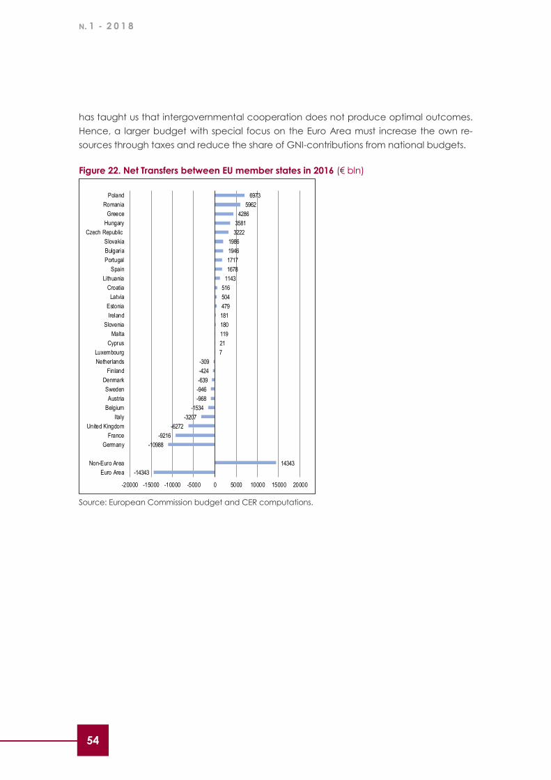
N. 1 - 2 0 1 8
54
has taught us that intergovernmental cooperation does not produce optimal outcomes.
Hence, a larger budget with special focus on the Euro Area must increase the own re-
sources through taxes and reduce the share of GNI-contributions from national budgets.
Figure 22. Net Transfers between EU member states in 2016 (€ bln)
Source: European Commission budget and CER computations.
-14343
14343
-10988
-9216
-6272
-3207
-1534
-968
-946
-639
-424
-309
7
21
119
180
181
479
504
516
1143
1678
1717
1946
1986
3222
3581
4286
5962
6973
-20000 -15000 -10000 -5000 0 5000 10000 15000 20000
Euro Area
Non-Euro Area
Germany
France
United Kingdom
Italy
Belgium
Austria
Sweden
Denmark
Finland
Netherlands
Luxembourg
Cyprus
Malta
Slovenia
Ireland
Estonia
Latvia
Croatia
Lithuania
Spain
Portugal
Bulgaria
Slovakia
Czech Republic
Hungary
Greece
Romania
Poland
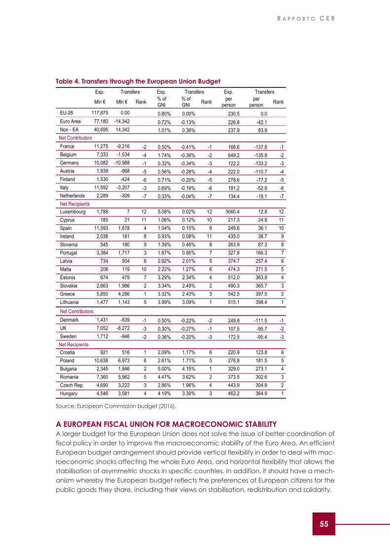
R A P P O R T O C E R
55 55
Table 4. Transfers through the European Union Budget
Source: European Commission budget (2016).
A EUROPEAN FISCAL UNION FOR MACROECONOMIC STABILITY
A larger budget for the European Union does not solve the issue of better coordination of
fiscal policy in order to improve the macroeconomic stability of the Euro Area. An efficient
European budget arrangement should provide vertical flexibility in order to deal with mac-
roeconomic shocks affecting the whole Euro Area, and horizontal flexibility that allows the
stabilisation of asymmetric shocks in specific countries. In addition, it should have a mech-
anism whereby the European budget reflects the preferences of European citizens for the
public goods they share, including their views on stabilisation, redistribution and solidarity.
Exp. Transfers Exp. Transfers Exp. Transfers
Mln € Mln € Rank % of GNI
% of GNI
Rank per
person per
person Rank
EU-28 117,875 0.00 0.80% 0.00% 230.5 0.0
Euro Area 77,180 -14,342 0.72% -0.13% 226.8 -42.1 Non - EA 40,695 14,342 1.01% 0.36% 237.9 83.9
Net Contributors
France 11,275 -9,216 -2 0.50% -0.41% -1 168.6 -137.8 -1
Belgium 7,333 -1,534 -4 1.74% -0.36% -2 649.2 -135.8 -2
Germany 10,082 -10,988 -1 0.32% -0.34% -3 122.2 -133.2 -3
Austria 1,939 -968 -5 0.56% -0.28% -4 222.0 -110.7 -4
Finland 1,530 -424 -6 0.71% -0.20% -5 278.6 -77.2 -5
Italy 11,592 -3,207 -3 0.69% -0.19% -6 191.2 -52.9 -6
Netherlands 2,289 -309 -7 0.33% -0.04% -7 134.4 -18.1 -7
Net Recipients
Luxembourg 1,788 7 12 5.08% 0.02% 12 3060.4 12.8 12
Cyprus 185 21 11 1.06% 0.12% 10 217.3 24.9 11
Spain 11,593 1,678 4 1.04% 0.15% 9 249.6 36.1 10
Ireland 2,038 181 8 0.93% 0.08% 11 435.0 38.7 9
Slovenia 545 180 9 1.39% 0.46% 8 263.9 87.3 8
Portugal 3,384 1,717 3 1.87% 0.95% 7 327.8 166.3 7
Latvia 734 504 6 2.92% 2.01% 5 374.7 257.4 6
Malta 208 119 10 2.22% 1.27% 6 474.3 271.5 5
Estonia 674 479 7 3.29% 2.34% 4 512.0 363.9 4
Slovakia 2,663 1,986 2 3.34% 2.49% 2 490.3 365.7 3
Greece 5,850 4,286 1 3.32% 2.43% 3 542.5 397.5 2
Lithuania 1,477 1,143 5 3.99% 3.09% 1 515.1 398.4 1
Net Contributors
Denmark 1,431 -639 -1 0.50% -0.22% -2 249.8 -111.5 -1
UK 7,052 -6,272 -3 0.30% -0.27% -1 107.5 -95.7 -2
Sweden 1,712 -946 -2 0.36% -0.20% -3 172.5 -95.4 -3
Net Recipients
Croatia 921 516 1 2.09% 1.17% 6 220.9 123.8 6
Poland 10,638 6,973 6 2.61% 1.71% 5 276.8 181.5 5
Bulgaria 2,345 1,946 2 5.00% 4.15% 1 329.0 273.1 4
Romania 7,360 5,962 5 4.47% 3.62% 2 373.5 302.6 3
Czech Rep. 4,690 3,222 3 2.86% 1.96% 4 443.9 304.9 2
Hungary 4,546 3,581 4 4.19% 3.30% 3 463.2 364.9 1

N. 1 - 2 0 1 8
56
Given, that the bulk of expenditure in the EU is allocated by national governments, a mech-
anism is needed to define the desired aggregate fiscal position (total public expenditure
minus revenue). This could be accomplished by first agreeing the aggregate fiscal stance
for the Euro Area in response to the prevailing macroeconomic conditions and then by
allocating borrowing rights to each member state.
The aggregate fiscal policy stance for the Euro Area should reflect the economic condi-
tions of the whole of European Monetary Union, but also collective preferences for the
allocation of resources, including their distribution between national and European public
goods. This would create a larger degree of fiscal flexibility, which is not possible with the
present rigid fiscal rules. However, once the aggregate deficit is defined at the European
level, each jurisdiction must be assigned a share of this total fiscal stance for implementa-
tion. Within their quota national governments would then set the priorities for collective
goods that reflect their voters’ preferences. For example, one country may prefer a large
public sector and therefore higher taxes, while another may opt for small government and
low taxes, but both must stick to the authorised net borrowing requirements.
Technically the procedure of first defining the macroeconomic aggregate and then its
micro application in a second step is well known in certain member states. For example,
the budget process in Italy defines first the multi-annual macroeconomic framework law,
the Documento di programmazione Economica e Finanziaria (DEF), and then the legge
finanziaria, which implements the actual budget allocations. Defining the aggregate Euro
Area fiscal stance would function like a European “DEF”. Because it affects all European
citizens, the responsibility for defining this aggregate Euro Area policy stance should be the
responsibility of the European Finance Minister (13).
Assigning quota for public borrowing to member states would depend on the size of coun-
tries, their economic situation, competitiveness conditions and the need to reduce public
debt. In accordance with the Treaty on European Union, defining such quota should be
the joint task of the European Finance Minister, the European Council and the European
Parliament.
The experience over the last two decades has proven that the voluntary cooperation
among the twenty-seven member states is no longer sufficient to generate and allocate
European public goods efficiently. This is undermining the legitimacy of the European Un-
ion. It is also becoming increasingly clear that in several member states government failure
and corruption prevent the fair and efficient employment of public funds. For this reason,
it is time to rethink the governance of European public goods. If failing governments are
part of the decision-making process and have veto rights, the policy output is unlikely to
achieve desirable results. Instead of intergovernmental cooperation, it may be a better
solution to provide certain public goods by a federal agency, which is acting on the basis
of competing legislation.
With these elements, a re-invented European Union would be able to keep its founding
promise: namely to preserve peace, increase welfare and bring people together.
(13) For further details of this proposal, see http://www.stefancollignon.de/PDF/OENBank.pdf

R A P P O R T O C E R
57 57
REFERENCES
Beetsma, R., Klaassen, F. & Giuliodori, M., 2008. The effects of public spending shocks on
trade balances and budget deficits in the European Union. Journal of the European
Economic Association, 6(2/3), pp. 414--423.
Belke, A. & Osowski, T., 2016. Measuring fiscal spillovers in the EMU and beyond: a global
VAR approach, s.l.: CEPS.
Caporale, G. M. & Girardi, A., 2013. Fiscal spillovers in the Euro Area. Journal of International
Money and Finance, 38((2013)), pp. 84.e1-84.e16.
Carreras, O., Kirby, S., Liadze, I. & Piggott, R., 2016. Fiscal policy spillovers, s.l.: National
Institute of Economic and Social Research.
Cavallo, A., Dallari, P. & Ribba, A., 2018. Fiscal policies in high debt Euro-Area countries.
s.l.:Springer.
Chudik, A. & Pesaran, H. M., 2015. Common correlated effects estimation of heterogenous
dynamic panel data models with weakly exogenous regressors. Journal of
Econometrics, 188(2), pp. 393-420.
Dees, S., Di Mauro, F., Pesaran, H. M. & Smith, V. L., 2007. Exploring the international linkages
of the euro area: a global VAR analysis. Journal of Applied Econometrics, 22(1), pp. 1--
38.
Dragomirescu-Gaina, C. & Philippas, D., 2015. Strategic interactions of fiscal policies in
Europe: a global VAR perpective. Journal of International Money and Finance, 59(2015),
pp. 49--76.
Eller, M., Martin, F. & Huber, F., 2017. How would a fiscal shock in Germany affect other
European countries? Evidence from a Bayesian GVAR model with sign restrictions. Focus
on European Economic Integration, Volume 1, pp. 54--57.
Fores, P., 2018. Monetary and Fiscal Policies Interaction in Monetary Unions. Journal of
Economic Surveys, February, 32(1), p. 226–248.
Furceri, D. & Zdzienicka, A., 2013. The Euro Area crisis: need for a supranational fiscal risk
sharing mechanism?, s.l.: International Monetary Fund.
Giavazzi, F., Jappelli, T. & Pagano, M., 1999. Searching for Non-Keynesian Effects of Fiscal
Policy CSEF (Centre For Studies In Economics And Finance) Working Paper no. 16
February 1999, Salerno: CSEF (Centre For Studies In Economics And Finance).
Hilbers, P., 2005. Interaction of Monetary and Fiscal Policies: Why Central Bankers Worry
about Government Budgets. In: Current Developments in Monetary and Financial Law.
Washington DC: IMF.
IMF, 2018. World Economic Outlook Update, Washington DC: International Monetary Fund.
Irish National Competitiveness Council, 2017. Ireland's Competitiveness Scorecard 2017,
Dublin: NCC.
Kempa, B. & Khan, N. S., 2017. Spillover effects of debt and growth in the euro area:
evidence from a GVAR model. International Review of Economics and Finance,

N. 1 - 2 0 1 8
58
49(2017), pp. 102--111.
McLeay, M., Amar, R. & Ryland, T., 2014. Money creation in the modern economy. Bank of
England Quarterly Bulletin , Volume Q1.
Nickel, C. & Vansteenkiste, I., 2013. The international spillover of fiscal spending on financial
variables. In: The GVAR handbook: Structure and applications of a macro model of the
global economy for policy analysis . s.l.:Oxford University Press, pp. 182--193.
Ramey, V. A., 2011. Can government purchase stimulate the economy?. Journal of
Economic Literature, 49(3), pp. 673--685.
Ricci-Risquete, A. & Ramajo-Hernandez, J., 2015. Macroeconomics effects of fiscal policy
in the European Union: a GVAR model. Empirical Economics, 48(2015), pp. 1587--1617.
Young, G., 2017. Commentary: Monetary and fiscal policy normalisation as Brexit is
negotiated. National Institute Economic Review , 242(November).
Zimmermann, T. & Hebous, S., 2013. Estimating the effects of coordinated fiscal actions in
the euro area. European Economic Review, 58(2013), pp. 110--121.


Rapporto CER
Re-inventing Europe
n.1 2018