MPRAMunich Personal RePEc Archive

Deconstructing the Gains from Trade:Selection of Industries vs. Reallocationof Workers

Stefano Bolatto and Massimo Sbracia

University of Turin, Bank of Italy

13. June 2014

Online at http://mpra.ub.uni-muenchen.de/56638/MPRA Paper No. 56638, posted 18. June 2014 23:48 UTC

Deconstructing the Gains from Trade:Selection of Industries vs. Reallocation of Workers*

Stefano Bolatto# and Massimo Sbracia§

June 2014

Abstract

In a Ricardian model with CES preferences and general distributions of industry

effi ciencies, the sources of the welfare gains from trade can be precisely decomposed into

a selection and a reallocation effect. The former is the change in average effi ciency due

to the selection of industries that survive international competition. The latter is the

rise in the weight of exporting industries in domestic production, due the reallocation of

workers away from less-effi cient non-exporting industries. This decomposition, which

is hard to calculate in the general case, simplifies dramatically if industry effi ciencies

are Fréchet distributed, providing easy-to-quantify model-based measures of these two

effects. Under this assumption, we also show that when the gains from trade are small,

it is the selection effect that matters most; as the gains from trade rise and the size of

the export sector grows, so does the importance of the reallocation effect.

JEL classification: F10, F11, F40

Keywords: Ricardian model; selection effect; reallocation effect

* We thank Guglielmo Caporale, Pietro Catte, Giuseppe De Arcangelis, Jonathan

Eaton, Alberto Felettigh, Andrea Finicelli and seminar participants at Penn State Univer-

sity (PSU) for many useful comments. Part of the paper was written while Stefano Bolatto

was visiting the Department of Economics at PSU, whose hospitality is gratefully acknowl-

edged. All the remaining errors are ours. The views expressed in this paper are those of

the authors and do not necessarily reflect those of the Bank of Italy. E-mail: stefanoanto-

nio.bolatto@unito.it, massimo.sbracia@bancaditalia.it.

# University of Turin, Dipartimento di Economia e Statistica "Cognetti de Martiis",

Lungo Dora Siena 100 A, 10153 Turin, Italy

§ Corresponding author: Bank of Italy, Via Nazionale 91, 00184 Rome, Italy (+39-06-

4792-3860)

1 Introduction

In a very influential paper, Arkolakis, Costinot, and Rodríguez-Clare (2012) have shown

that the welfare gains from trade implied by a very large class of models depend on

only two suffi cient statistics: (i) the share of expenditure on domestic goods (which is

often called "domestic trade share"); and (ii) the elasticity of imports with respect to

variable trade costs ("trade elasticity"). This result is remarkable because it applies

to frameworks as different as the simple Armington model, in which goods are differ-

entiated by country of origin; the Ricardian model with heterogeneous industries and

Fréchet-distributed effi ciencies of Eaton and Kortum (2002); the monopolistic compe-

tition model of Krugman (1980); as well as variants of the monopolistic competition

model of Melitz (2003), with heterogeneous firms and Pareto-distributed effi ciencies

(such as those developed by Chaney, 2008, and Eaton, Kortum, and Kramarz, 2011).

Given their importance for empirical studies, these models are now commonly referred

to as "quantitative trade models."

Following this result, the literature appears to be taking two main directions. One

analyzes how the measurement of the gains from trade changes when some assumptions

of quantitative trade models are relaxed (see Arkolakis, Costinot, Donaldson, and

Rodríguez-Clare, 2012, and Melitz and Redding, 2013 and 2014). The other focuses on

the empirical implications of the result. In particular, it is now clear that the various

models have different implications for the estimated value of the trade elasticity, so

that even though the analytical formulation of the gains from trade is the same, the

resulting quantification still differs across models (Simonovska and Waugh, 2014a).

In this paper we explore a different route, by focusing on the sources of the

welfare gains of the open economy with respect to the autarky economy. In particular,

we study whether quantitative trade models allow us to quantify not only the overall

welfare gains, but also the contribution of the different sources. This is a key issue in

both the theoretical and the empirical literature in international trade. The matter is

also critical for policy purposes. By understanding what are the most important sources

of the welfare gains, countries could design and implement appropriate policies in order

to maximize the benefits from trade liberalization and foster economic development.

Answering this question, however, is in general very diffi cult, because different

quantitative models entail different predictions on the sources of the welfare gains.

For example, gains from consuming a greater variety of goods are key in Armington

and monopolistic competition models, but are absent in Ricardian models. Given

these sharp differences, we analyze this question for one specific family of models and

investigate whether belonging to the class of quantitative trade models facilitates the

1

measurement of the contribution of the different sources.

The family on which we focus is the Ricardian model with many countries and

goods, CES preferences, and general distributions of industry effi ciencies. Thus, with

respect to Arkolakis, Costinot, and Rodríguez-Clare (2012), although we restrict the

attention to only one family of models, we extend the scope of the analysis by providing

general results for Ricardian models in which industry effi ciencies follow a generic

distribution, and not necessarily a Fréchet.

For this general family of models, we show that the welfare gains of the open

economy with respect to the autarky economy can always be decomposed into two

distinct sources: a selection and a reallocation effect. The former is the effect on average

effi ciency of the selection of industries that, thanks to their suffi ciently low marginal

costs of production relative to foreign industries, survive international competition.

Such average effi ciency is computed by considering, for the sole industries that survive

international competition, the same relative weights in domestic production as the

autarky economy. The latter effect, instead, is related to the rise in the weight in

domestic production of the exporting industries, which is due to the reallocation of

workers away from the less-effi cient non-exporting industries to the industries that

start servicing the foreign market.

While the model provides very precise theoretical definitions for both effects,

their analytical expression is, in general, too cumbersome to be used for empirical

purposes. In most applications, in fact, it would require computing several billions

of distributions of effi ciencies. By contrast, this decomposition simplifies dramatically

if we impose that industry effi ciencies are Fréchet distributed – the assumption that

makes our Ricardian model belong to the class of quantitative trade models. Under

this assumption, we can derive exact model-based measures of these two effects, which

can be quantified using only data on trade flows and domestic production.

The Fréchet assumption entails this simplification for the following reasons. First,

it allows us to easily quantify the gains from trade, as shown by Arkolakis, Costinot,

and Rodríguez-Clare (2012). Second, it implies that the selection effect is a measurable

share of the overall gains from trade, making it possible to obtain the contribution to

welfare of this effect. Third, as a consequence, the reallocation effect (whose quan-

tification is, in the general case, extremely diffi cult) can be calculated simply as the

complement of the selection effect. Therefore, a key insight of our analysis is that quan-

titative trade models seem to be useful not only to assess the overall welfare gains, but

also to properly measure their sources.

Using the Fréchet assumption, we also demonstrate that, when the gains from

trade are small and there are still few exporters in the domestic economy, the largest

2

share of the welfare gains is due to the selection effect. As the export sector grows

and the gains from trade increase, the importance of the reallocation effect also rises.

Because the contribution of the reallocation effect rises with the size of the overall

gains from trade, it follows that the factors affecting the former are exactly the same

factors affecting the latter. In particular, both the welfare gains and the contribution

of the reallocation effect are higher for small, open and very productive economies,

located near to markets that are large, rich, and less productive and, therefore, easier

to penetrate. Another interesting feature of our result is that the specific value of the

trade elasticity, which is key to determine the overall welfare gains, does not affect the

shares of the gains pertaining to the selection and the reallocation effect, making their

measurement even more straightforward and robust than that of the welfare gains.

A quantification for a sample of 46 advanced and developing economies in the

years 2000 and 2005 shows that the selection effect is, on average, somewhat more

important than the reallocation effect (accounting for about 60% of the gains from

trade). In particular, the selection effect is dominant for large countries: only in

the United States and Japan, among the advanced economies, and in Brazil, Russia,

India, and China, among the developing countries, does the share of gains pertaining

to the selection effect exceeds 80 percent. However, for small open economies such

as Denmark, Ireland, the Netherlands, Singapore, Thailand, and Vietnam, it is the

reallocation effect that is dominant, as it is responsible for over 70 percent of the gains.

These findings have important policy implications. Suppose that the export sector

is less similar to other sectors of the economy in terms of, for example, skills that are

required to workers, as documented by the empirical literature.1 This feature of the

export sector could make resource reallocation from other industries slower or more

diffi cult. In this case, our theoretical and empirical results suggest that, in the initial

stages of trade liberalization (i.e. when trade barriers are still high), these frictions do

not prevent to reap the benefits from trade, because most of the gains obtain from the

selection effect, that is from the closure of less effi cient industries and the reallocation of

workers across all the surviving industries, which are mostly non-exporters. Similarly,

large countries can expect to enjoy welfare gains almost in full, even in the hypothesis

of a cumbersome reallocation to the export sector, thanks to the considerable size of

their non-exporting industries. On the other hand, reallocation of workers to the export

sector is crucial in small open economies. Therefore, to fully benefit from trade, these

countries must be ready to favor resource reallocation to this sector, in particular by

enhancing education and training for unskilled workers.

1Bernard, Jensen, Redding and Schott (2007) show, in fact, that exporting firms are more skill

intensive than their domestic competitors.

3

Our paper is related to several strands of the literature. Many recent empiri-

cal and theoretical studies have focused on one specific source of the welfare gains,

that is aggregate productivity. An early example is Pavcnik (2002), who estimates

productivity improvements in Chile using firm-level data. This study confirms the im-

portance of the mechanisms described in this paper, as it finds that the exit of plants

and the reshuffl ing of resources from less effi cient to more effi cient producers are the

main sources of the productivity gains. Many other papers, instead, have focused on

model-based measures of the "productivity gains from trade," computed as increases

in average effi ciency.2 To better grasp the link between these papers and our own, it

is worth recalling that, in the Ricardian model, the growth in world-wide aggregate

productivity induced by international trade is the basic source of the welfare gains for

all countries. In other words, countries benefit from the fact that, by specializing in the

production of the goods for which they have a comparative advantage, the world pro-

duction of the optimal consumption bundle increases. Thus, our paper sheds light on

how each individual country, through the mechanisms of selection and reallocation in-

duced by trade liberalization, contributes to the improvement in world-wide aggregate

productivity and reaps the benefits of international trade for its own welfare.

Another related strand of the literature is the wave of papers focusing on empir-

ical estimates of the gains from trade, such as Feenstra (1994 and 2010), Broda and

Weinstein (2006), Goldberg, Khandelwal, Pavcnik, and Topalova (2009), and many

others. These papers use different econometric techniques to quantify either the con-

tribution of specific sources of gains (usually those from consuming new varieties) or

the size of the overall welfare gains. Our approach, instead, grounded on the derivation

of model-based measures of the welfare gains, follows more closely the one of Eaton

and Kortum (2002), Alvarez and Lucas (2007), Arkolakis, Demidova, Klenow, and

Rodríguez-Clare (2008), Ravikumar and Waugh (2009), and Arkolakis, Costinot, and

Rodríguez-Clare (2012). Unlike those papers, however, we are also able to quantify the

contribution of the different sources of gains.3

Given that a big chunk of the related literature focuses on welfare gains in mo-

2See, for example, Bernard, Eaton, Jensen, and Kortum (2003), Costinot, Donaldson, and Ko-

munjer (2012), Bolatto (2013), Finicelli, Pagano and Sbracia (2013a and 2013b), and Levchenko and

Zhang (2013).

3A close relative of our study is also the paper by Demidova and Rodríguez-Clare (2009), who

decompose the welfare gains from trade of a small open economy under monopolistic competition

into four terms: productivity, terms of trade, number of varieties, and curvature (i.e. the degree of

heterogeneity across varieties). Here, instead, we consider a general equilibrium model with perfect

competition and, most importantly, we derive a quantifiable expression of the two sources that, in our

Ricardian framework, provide the welfare gains.

4

nopolistic competition models à la Melitz (2003), it is worth clarifying the differences

between these frameworks and the Ricardian one. On the production side, the adjust-

ment that takes place after trade liberalization is very similar in the two frameworks.

In both models, in fact, domestic production: (i) focuses only on a subset of the goods

that were made under autarky (these are the goods that are made more effi ciently with

monopolistic competition, and those in which the country has a comparative advantage

in Ricardo); (ii) becomes tilted towards exporters (who benefit from foreign demand).

On the consumption side, according to both models households consume less of those

tradeable goods whose production remains domestic; however: (a) in the Ricardian

model, households purchase more of the remaining tradeable goods (because imports

are cheaper), so that overall consumption increases, even though they do not gain

access to more varieties; (b) in the monopolistic competition model, households start

consuming a greater variety of goods. For any country, if the trade elasticity implied

by the two models were the same, then the gain from consuming a larger quantity of

imported goods in the Ricardian model would be the same as the gain from consuming

more imported varieties in frameworks à la Melitz (2003). To put it differently, with

identical trade elasticities, "Ricardo’s intensive margin" would be equal to "Melitz’s

extensive margin".4

The rest of the paper is organized as follows. Section 2 describes the model, which

extends Eaton and Kortum (2002) to general distributions of industry effi ciencies. Sec-

tion 3 shows that the welfare gains induced by international trade can be decomposed

into two distinct effects, related to the selection of industries and the reallocation of

workers. Section 4 introduces the assumption of Fréchet-distributed industry effi cien-

cies, shows that the analytical expressions of the two effects simplify, and quantifies

them for a sample of countries and years. Section 5 draws the main conclusions.

4We recall, however, the important caveat, established by Simonovska and Waugh (2014a), that

different trade models have different implications about the value of the trade elasticity. These authors,

in particular, report point estimates of the trade elasticity that are in a range between 4.0 and 4.6

for the Eaton-Kortum model (see their tables 2 and 3) and between 3.6 and 3.7 for the Melitz model

(table 4). This result would imply that welfare gains (which are decreasing in the trade elasticity)

are somewhat higher in the latter model. Nevertheless, the empirical question concerning the value of

the trade elasticities (and, in turn, of the gains from trade) in the two models seems to be still wide

open. Other papers, in fact, do find lower values of the trade elasticity for the Eaton-Kortum model,

reporting estimates as low as 3.6 (Eaton and Kortum, 2002) and 2.8 (Simonovska and Waugh, 2014b).

5

2 The model

We consider a continuum of tradable goods, indexed by j ∈ [0,+∞), that can poten-

tially be produced in any of the N countries of the world economy. Each good j can be

produced in country i with an effi ciency zi (j) that, in turn, is defined as the amount of

output that can be produced with one unit of input – where both output and input

are measured in units of constant quality. Any country has a fixed labor endowment Li.

Inputs include labor as well as a bundle of intermediates goods, which comprises the

full set of tradable goods j.5 Technology is described by a Cobb-Douglas production

function with constant returns to scale, in which labor has a constant share β ≤ 1 for

all industries and countries; namely:

qi (j) = zi (j)Lβi (j) I1−βi (j) , (1)

where qi (j) is the quantity of output j in country i, Li (j) is the number of workers,

and Ii (j) is the quantity of the bundle of intermediate goods.

Consumer preferences are the same across countries. The representative consumer

in country i purchases individual goods in amounts ci(j) in order to maximize a CES

utility function:

Ui =[∫

[ci(j)]σ−1σ dj

] σσ−1

,

where σ > 0 is the elasticity of substitution. While the model allows us to deal with

both inelastic (σ ≤ 1) and elastic demand (σ > 1), we will focus on the latter case,

because the goods that we consider are all tradable and, in this setting, the typical

calibration is σ > 1.6

Consumers maximize their utility function subject to a standard budget con-

straint. Because we assume that trade is balanced in the open economy, income avail-

able for consumption is Yi = wiLi, where wi is the (nominal) wage.

International trade is constrained by barriers, which are modeled using the stan-

dard assumption of iceberg costs; i.e., delivering one unit of a good from country i to

country n requires shipping dni units, with dni > 1 for i 6= n and dii = 1 for any i. By

arbitrage, trade barriers obey the triangle inequality, so that dni ≤ dnk · dki for any n,i and k.

Perfect competition implies that the price of one unit of good j produced by

5We can ignore physical capital in the production function because the model is static and, then,

intermediate inputs play a very similar role.

6For an extension of the model that encompasses both tradable and non-tradable goods, see Di

Nino, Eichengreen, and Sbracia (2013).

6

country n and delivered to country i is:

pin (j) =cndinzn (j)

,

where cn = wβnp1−βn is the cost of one unit of input in the source country n, with pn

being the unit price of the optimal bundle of intermediate goods, which is the same as

the unit price of the optimal bundle of final goods (see equation (3) below). In other

words, we assume (as Eaton and Kortum, 2002) that producers combine intermediate

goods using the same CES aggregator that consumers use to combine final goods.

Consumers purchase each good from the country that can supply it at the lowest

price; therefore, the price of good j in country i is:

pi (j) = minn

(cndinzn (j)

).

We assume that, in each country i, industry effi ciencies zi(j) are the realiza-

tions of a random variable Zi, with a country-specific cumulative distribution function

(c.d.f.) Fi. Because the zi (j) represent industry effi ciencies and there is a continuum

of goods, it is natural to assume that Zi is non-negative and absolutely continuous

for each country i. These are the only conditions that we impose, in this and in the

following section, on the Zi’s (in Section 4, instead, we assume that the Zi are Fréchet

distributed). As the expert reader may have noticed, we do not impose the standard

restriction that the Zi are mutually independent across countries, but we allow for

dependent (correlated) variables.

The continuum-of-goods assumption and the conventional application of the law

of large numbers imply that the share of goods for which country i’s effi ciency is below

any real number z is the probability Pr (Zi < z) = Fi (z). It is worth noting that,

in the autarky economy, all goods are made at home and, then, Zi is the effi ciency

distribution of the closed economy.

Given the cost of inputs, the distribution of industry effi ciencies translates into a

distribution of good prices. More formally, let us denote with Pi the random variable

that describes the distribution of good prices in country i; this random variable is

defined as:

Pi = minn

(cndinZn

)=

[maxn

(Zncndin

)]−1. (2)

The price index in country i, pi, computed using the correct CES aggregator, is simply

the moment of order 1− σ of the random variable Pi, at the 1/ (1− σ) power; that is:

pi =[E(P 1−σi

)]1/(1−σ). (3)

7

After a simple manipulation of equations (2) and (3), we obtain:

pi = ci ·[E(Mσ−1

i

)]1/(1−σ),

where Mi = maxn

(cicn

Zndin

), (4)

that leads to the real wage, which measures welfare:7

wipi

=[E(Mσ−1

i

)]1/β(σ−1). (5)

The welfare gain from trade can be obtained by comparing the real wage of the

open and the closed economy, where the latter can be obtained from the former, letting

din → +∞ for i 6= n (using equations (4) and (5)). In this case, we have Mi → Zi and

the real wage is[E(Zσ−1i

)]1/β(σ−1). Hence, the gain from trade for country i is:

gi =

[E(Mσ−1

i

)E(Zσ−1i

) ]1/β(σ−1) . (6)

Equation (6) shows that the welfare gain arises from the transformation, that occurs

in the open economy, of the "source of the production effi ciencies" (effi ciencies that,

in turn, determine good prices) from Zi to Mi. Note, in particular, that the latter

random variable is a maximum between a set of random variables that includes also Zi.

Because the maximum of a set of random variables first-order stochastically dominates

any variable included in the set, then Mi Zi, so that gi ≥ 1.8 In other words,

the real wage is higher in the open economy. Thus, the result that trade is welfare

improving is here proven using the language of probability, rather than the tools of

general equilibrium.9

3 Welfare decomposition

Let us now focus on how labor units are reallocated after opening to trade. To fos-

ter intuition, we start by considering the case of two countries, say i and n, before

generalizing the result to N countries.

7Recall that, in the competitive equilibrium of both the open and the closed economy, welfare is

wiLi/pi, where Li is exogenous.

8We remind the reader that the random variable X first-order stochastically dominates the random

variable Y , and we write X Y , if and only if FX (z) ≤ FY (z) for any z ∈ R, where FX and FY are

the c.d.f. of, respectively, X and Y . If this condition holds, then E(Xk)≥ E

(Y k), for any k > 0.

9The finding that gi ≥ 1 for any i, proven using basic probability theory, generalizes a result of

Finicelli, Pagano, and Sbracia (2013a), extending it to a framework in which there are also intermediate

goods.

8

3.1 A 2-country example

The first-order conditions (FOCs) of the consumer’s problem imply that the consump-

tion of good j in country i is:

ci (j) =

[pi (j)

pi

]−σ· Ui , (7)

where Ui = wiLi/pi is the level of utility achieved by country i.

The FOCs of the producer’s problem, on the other hand, imply that the quan-

tities of labor and intermediate goods used to produce good j in country i are chosen

according to the following proportions:

Ii (j) =1− ββ

wipiLi (j) . (8)

By aggregating across industries both sides of equation (8), we find that the overall

amount of intermediate goods used in country i is Ii = 1−ββ· (wi/pi) · Li.

The assumption that intermediate goods are combined using the same CES ag-

gregator used to combine final goods implies that, for any country i, the demand for

j as intermediate good, mi (j), is proportional to the demand as consumption good,

ci (j); that is: ci (j) /Ui = mi (j) /Ii. Because Ii/Ui = (1− β) /β, it follows that, in

country i, the demand for good j as an intermediate input is mi (j) = (1− β) ·ci (j) /β.Hence, in any country i, the overall demand for good j is ci (j) /β.

In the two-country model that we are examining, each good can either be pro-

duced abroad and imported at home; or be produced at home and sold only in the

domestic market; or be produced at home and sold both in the domestic and the

foreign market. Therefore, the resource constraint for country i requires that:

qi (j) =

0 if j ∈ Oi,z

1βci (j) if j ∈ Oi,d

1β

[ci (j) + cn (j) dni] if j ∈ Oni,e

, (9)

for any j, where Oi,z denotes the set of "zombie" industries of country i, i.e. those

industries that shut down right after trade liberalization;10 Oi,d is the set of industries

that sell their goods only on the domestic market; and Oni,e is the set of industries

that sell both at home and in country n.11 By construction, the sets Oi,z, Oi,d, and

10We borrow the terminology "zombie industries" from Caballero, Hoshi, and Kashyap (2008), who

use it to refer to industries that are kept alive only by misdirected or subsidized bank lending. In the

context of our model, instead, these industries would be kept alive by trade protectionist policies.

11In the two-country model, these sets are defined as follows: Oi,z =j : zi(j)ci

> zn(j)cndin

, Oi,d =

j : zn(j)cndin

≤ zi(j)ci

> zn(j)dnicn

, and Oni,e =

j : zi(j)ci

≥ zn(j)dnicn

.

9

Oni,e form a partition of the set of tradable goods; hence, the intersection between any

subset of them is empty and their union spans the whole set of tradable goods. The

set Oi,o ≡ Oi,d ∪ Oni,e, on the other hand, includes the sole industries that survive

international competition.12

By plugging equations (1) and (7) into equation (9) (using also equation (8)),

and solving the resource constraint for the number of workers in industry j, we obtain:

Li (j) =

0 if j ∈ Oi,z

zσ−1i (j) ·(wipi

)β(1−σ)Li if j ∈ Oi,d

zσ−1i (j) ·(wipi

)β(1−σ)Li · (1 + kni) if j ∈ On

i,e

, (10)

where:

kni =wnLnwiLi

(pidnipn

)1−σ. (11)

The term kni measures the rise in the weight of the exporting relative to non-exporting

industries. It is related to the demand that comes from country n, since it depends

positively on the size of this country in terms of relative GDP, and negatively on the

iceberg cost between countries i and n, and their relative price levels.

In the autarky economy, Oi,z = Oni,e = ∅ and the resource constraint returns, for

any good j, Li (j) = zσ−1i (j) · (wi/pi)β(1−σ) Li. Let us consider, then, how labor is re-allocated after trade liberalization. With respect to the autarky economy, in the open

economy the number of workers in the zombie industries goes to zero. The number of

workers in the industries that produce goods that are sold only domestically declines

(provided that σ > 1), because these industries face a tougher competition, due to the

fact that imported goods are cheaper than those that were made at home under the

autarky regime.13 The number of workers in the exporting industries rises, absorb-

ing all the workers "in excess" from the other domestic industries. More specifically,

these industries sell less in the domestic market (as international competition brings

in cheaper imported goods), so they would need less workers to serve this market, but

foreign demand allows them not only to keep their workers, but also to hire new ones

in order to produce more goods to be sold abroad.14

12The term cn (j) dni/β in equation (9) represents the foreign demand that benefits only the export-

ing industries. In particular, the representative consumer of country n demands the quantity cn (j) /β,

but iceberg costs imply that dni units must be shipped from country i to deliver one unit of good to

country n. Thus, the overall quantity produced to serve the latter market is cn (j) dni/β.

13If σ < 1 (σ = 1), industries producing goods that are sold only at home would employ more (the

same number of) workers.

14For j ∈ Oni,e, the two terms of equation (10) represent exactly these factors: the number of workers

10

Notice that, in any industry, the number of workers is proportional to the effi -

ciency of this industry, at the σ − 1 power (i.e. to zσ−1i (j)). By aggregating across

industries both sides of equation (10), we can derive the following decomposition of the

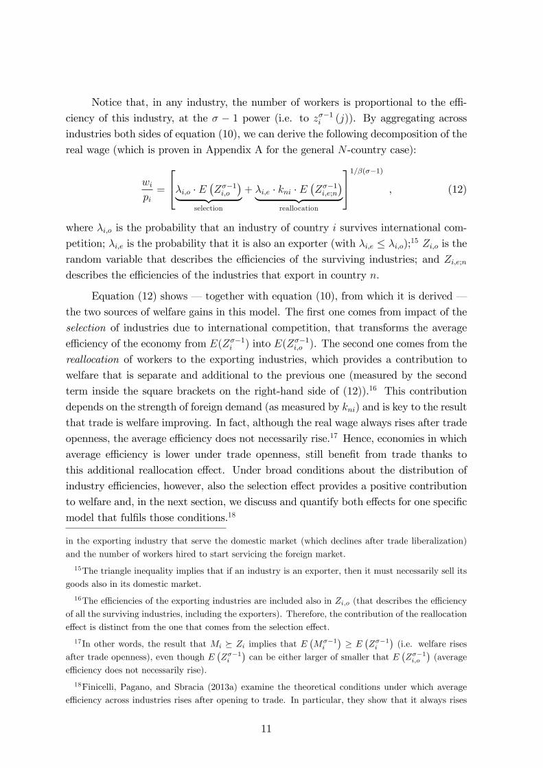
real wage (which is proven in Appendix A for the general N -country case):

wipi

=

λi,o · E (Zσ−1i,o

)︸ ︷︷ ︸selection

+ λi,e · kni · E(Zσ−1i,e;n

)︸ ︷︷ ︸reallocation

1/β(σ−1) , (12)

where λi,o is the probability that an industry of country i survives international com-

petition; λi,e is the probability that it is also an exporter (with λi,e ≤ λi,o);15 Zi,o is the

random variable that describes the effi ciencies of the surviving industries; and Zi,e;ndescribes the effi ciencies of the industries that export in country n.

Equation (12) shows – together with equation (10), from which it is derived –

the two sources of welfare gains in this model. The first one comes from impact of the

selection of industries due to international competition, that transforms the average

effi ciency of the economy from E(Zσ−1i ) into E(Zσ−1

i,o ). The second one comes from the

reallocation of workers to the exporting industries, which provides a contribution to

welfare that is separate and additional to the previous one (measured by the second

term inside the square brackets on the right-hand side of (12)).16 This contribution

depends on the strength of foreign demand (as measured by kni) and is key to the result

that trade is welfare improving. In fact, although the real wage always rises after trade

openness, the average effi ciency does not necessarily rise.17 Hence, economies in which

average effi ciency is lower under trade openness, still benefit from trade thanks to

this additional reallocation effect. Under broad conditions about the distribution of

industry effi ciencies, however, also the selection effect provides a positive contribution

to welfare and, in the next section, we discuss and quantify both effects for one specific

model that fulfils those conditions.18

in the exporting industry that serve the domestic market (which declines after trade liberalization)

and the number of workers hired to start servicing the foreign market.

15The triangle inequality implies that if an industry is an exporter, then it must necessarily sell its

goods also in its domestic market.

16The effi ciencies of the exporting industries are included also in Zi,o (that describes the effi ciency

of all the surviving industries, including the exporters). Therefore, the contribution of the reallocation

effect is distinct from the one that comes from the selection effect.

17In other words, the result that Mi Zi implies that E(Mσ−1i

)≥ E

(Zσ−1i

)(i.e. welfare rises

after trade openness), even though E(Zσ−1i

)can be either larger of smaller that E

(Zσ−1i,o

)(average

effi ciency does not necessarily rise).

18Finicelli, Pagano, and Sbracia (2013a) examine the theoretical conditions under which average

effi ciency across industries rises after opening to trade. In particular, they show that it always rises

11

Before turning to the quantification, however, let us show how the result gener-

alizes to the case of many countries (N ≥ 2).

3.2 The N-country case

For the general multi-country framework, in Appendix A we prove that the real wage in

each country i has still two components, the selection effect (SEi) and the reallocation

effect (REi):wipi

= (SEi +REi)1/β(σ−1) . (13)

The first term inside the brackets of the right hand side of (13) has the same expression

as the corresponding term of the two-country case:

SEi = λi,o · E(Zσ−1i,o

). (14)

The second term is now more cumbersome:

REi =∑n6=i

λi,e;n · kni · E(Zσ−1i,e;n

)+

+∑

n 6=i,h 6=i,n 6=h

λi,e;n,h · (kni + khi) · E(Zσ−1i,e;n,h

)+

+...+ λi,e;1,...,N · (k1i + ...+ kNi) · E(Zσ−1i,e;1,...,N

), (15)

where λi,e;n,h,...,k is the probability that an industry of country i exports in (and only)

countries n, h, ..., and k; while Zi,e;n,h,...,k is the distribution of the effi ciencies of these

industries.

As shown by equations (12) and (15), in both the cases N = 2 and N > 2 the

magnitude of the reallocation effect is governed by kni (equation (11)). In particular,

kni and the size of the reallocation effect are larger if country i is relatively more

productive (pi/pn is low), and if the destination market n is rich (wn/wi high), large

(Ln is high relative to Li) and not too far away (dni low). Thus, geography, which is

key in the Ricardian model as shown by Eaton and Kortum (2002), exerts its effects

mostly through the reallocation of workers to the export sector.

In principle, quantifying the expressions of (14) and (15) is not an impossible task,

although it may be rather daunting. Given the joint distribution of (Z1, ..., ZN), in fact,

under very broad assumptions about the country distributions of industry effi ciencies; namely: (i) if

the distributions of effi ciencies are independent across countries; (ii) for many types of distributions,

if their correlations are suffi ciently low; (iii) regardless of cross-country correlations, if industry effi -

ciencies belong to families of distributions that are widely used in the literature, such as the Fréchet,

Pareto and Lognormal.

12

one can always derive the distribution of any of the Zi,e;n,h,...,k, which are just univariate

conditional distributions (see Appendix A). However, in empirical applications their

number might be extremely large, making their computation a very challenging task.

With N countries, one has to compute the distributions of the effi ciencies for the

industries that export in each of the N − 1 foreign countries, those for the industries

that export in all the possible N (N − 1) /2 couples of countries, etc.. For instance,

in the 46-country application that we consider in the next section, one should have to

compute a total of more than 35,000 billions of different distributions (that is 2N−1−1).

In the next section, instead, we show that, by introducing an assumption that transform

our general Ricardian model into one of the quantitative trade models of Arkolakis,

Costinot, and Rodríguez-Clare (2012), the quantification of the two effects simplifies

dramatically.

4 Fréchet-distributed effi ciencies

We now assume that, in any country i, industry effi ciencies are Fréchet distributed,

with parameters Ti and θ;19 hence, the probability that an industry of country i has an

effi ciency lower that a positive real number z is Fi(z) = exp−Tiz−θ

. For the sake

of simplicity, we also assume that these distributions are mutually independent across

countries.20

The moment of order k of Zi is:

E(Zki

)= T

k/θi · Γ

(θ − kθ

), (16)

which exists if and only if θ > k, where Γ is Euler’s Gamma function. Because welfare

is related to the moment of order σ− 1 of Zi, we assume θ > σ− 1. The parameter Ti,

usually defined as the "state of technology" of country i, captures country i’s absolute

advantage: an increase in Ti relative to Tn implies an increase in the share of goods

that country i produces more effi ciently than country n. The shape parameter θ,

19Kortum (1997) and Eaton and Kortum (2009) show that the Fréchet distribution emerges from

a dynamic model of innovation in which, at each point in time: (i) the number of ideas that arrive

about how to produce a good follows a Poisson distribution; (ii) the effi ciency conveyed by each idea

is a random variable with a Pareto distribution; (iii) firms produce goods using always the best idea

that has arrived to them.

20The key assumption is that industry effi ciencies are Fréchet distributed, while independence can

easily be relaxed. In particular, Eaton and Kortum (2002) propose a multivariate Fréchet distribution

for industry effi ciencies that allows for correlation across countries, and Finicelli, Pagano and Sbracia

(2013a) use it to compute the "productivity gains from trade" for different degrees of correlation.

13

common to all countries, is inversely related to the dispersion of Zi. It is related to the

concept of comparative advantage because, in the Ricardian model, gains from trade

depend on the heterogeneity in effi ciencies. In this model, a decrease in θ (i.e. higher

heterogeneity), coupled with mutual independence, generates larger gains from trade

for all countries.

An important property of the model with Fréchet-distributed effi ciencies is that

the price distribution in country i for the goods imported from country n is the same

for any n (and equal to Pi). Thus, for example, source countries with a higher state of

technology or lower iceberg costs exploit these advantages by selling a wider range of

goods to that country but, in the equilibrium, the price distributions of the goods that

the various foreign sources supply to the destination market i are identical (see Eaton

and Kortum, 2002, and Arkolakis, Costinot, and Rodríguez-Clare, 2012). A related

key property is that, in the open economy: Mi = Zi,o.21 Hence, equation (5) becomes:

wipi

=[E(Zσ−1i,o

)]1/β(σ−1). (17)

We now show how the analytical decomposition of welfare simplifies and how its

sources can be quantified under the Fréchet assumption. Combining equation (17) with

(13) and using equation (14), it turns out that:

REi = (1− λi,o) · E(Zσ−1i,o

), (18)

while it is still SEi = λi,o · E(Zσ−1i,o

).

The welfare gain induced by trade openness (equation (6)) becomes:

gi =

[E(Zσ−1i,o

)E(Zσ−1i

)]1/β(σ−1) ,that, in turn, can be decomposed as:

gi =

λi,o · E(Zσ−1i,o

)E(Zσ−1i

)︸ ︷︷ ︸selection

+ (1− λi,o) ·E(Zσ−1i,o

)E(Zσ−1i

)︸ ︷︷ ︸reallocation

1/β(σ−1)

.

In other words, given the overall gain from trade gi, a share λi,o of the gain is due to

the selection effect, while its complement, 1− λi,o, is due to the reallocation effect.22

21If the random variables X ∼ Frechet (ξ, θ) and Y ∼ Frechet (λ, θ) are independent, then

max (X,Y ) ∼ X|X ≥ Y ∼ Frechet (ξ + λ, θ).

22In interpreting the shares of the welfare gain due to the selection and the reallocation effect, we can

14

We can now turn to the measurement. The properties of the Fréchet distribution

imply that Zi,o is still a Fréchet, with parameters Λi and θ, where:23

Λi = Ti +∑i 6=k

Tk

(ckdikci

)−θ.

It follows that:24E(Zσ−1i,o

)E(Zσ−1i

) =

(Λi

Ti

)(σ−1)/θ.

To quantify gi, we borrow from Finicelli, Pagano and Sbracia (2013a, Proposition 5)

the result that:

Λi = Ti · Ωi

where Ωi ≡ 1 +IMP i

PROi − EXP i

, (19)

in which IMPi is the value of country i’s aggregate imports, PROi is the value of its

production, and EXPi is the value of aggregate exports. Thus:

gi = (Ωi)1/βθ . (20)

This is the same result established by Arkolakis, Costinot, and Rodríguez-Clare (2012)

for the larger class of quantitative trade models. In fact, Ω−1i , which is equal to one

minus the import penetration ratio, is the so-called "trade domestic share" (i.e. the

share of expenditure on domestic goods), while in this Ricardian model the trade

elasticity is βθ.

The quantification of the selection and the reallocation effect can be completed

once that we derive λi,o, which is the probability that an industry of country i survives

international competition. Using the properties of the Fréchet distribution, it is easy

to find that:

λi,o =Ti (ci)

−θ∑k Tk (ckdik)

−θ =1

Ωi

(21)

safely ignore the complication due to the exponent 1/β (σ − 1). In fact, a monotone transformation of

the utility function, such as the one that can be obtained by taking Ui at the β (σ − 1) power, would

yield the same equilibrium quantities and relative prices. In this transformed model, then, welfare

would be the same as in the original model, but at the β (σ − 1) power, making the exponent of the

gain from trade equal to 1 (while leaving the base unchanged).

23The result follows immediately from the property described in footnote 22 and the fact that if

X ∼ Frechet (ξ, θ) and a > 0, then aX ∼ Frechet(aθξ, θ

).

24Note that Λi > Ti. In other words, if industry effi ciencies are Fréchet distributed, then the average

effi ciency of the surviving industries is always higher than that of the whole set of domestic industries

(i.e. of the set that includes also the industries that shut down after trade liberalization). This feature

of the "quantitative Ricardian trade model" is both consistent with the available empirical evidence

and it is shared by a large class of Ricardian models (see footnote 15).

15

Note that, because welfare gains are increasing in Ωi, it follows that, when gains

are larger, the selection effect is less important and the reallocation effect is more

important. This result can be readily explained. When gains from trade are small, the

selection effect matters mostly because there are few exporters in the domestic economy

and, then, the possibilities of reallocating workers in these industries are fewer. On

the other hand, as the export sector grows and the gains from trade increase, the

importance of the reallocation effect also rises because exporting industries (which are

on average more productive) absorb more workers.

What does real data show about the size of these two effects? Table 1 provides

a quantification of the welfare gains from trade as well as the contribution of the

selection and reallocation effect for a sample of 46 advanced and developing countries

in two different years, 2000 and 2005. Gains are computed using equation (20), taking

the value of the main parameters from literature. In particular, we assume that the

shape parameter is θ = 4, as advocated by Simonovska and Waugh (2014b), and the

share of intermediate goods in production is β = 0.33, a conventional measure of the

share of value added in total output. The share of the gains from trade pertaining

to the selection and reallocation effects, respectively equal to λi,o and 1 − λi,o, are

computed using equation (21).

Given that the Ricardian theory laid out in this paper best describes trade in

manufactures, rather than in natural resources or primary goods, we follow the litera-

ture and consider data on the values of domestic production, exports and imports –

which is all is needed to compute the gains from trade as well as the contribution of

their sources – all referred to the manufacturing sector. In addition, given that the

model assumes that trade is balanced, in the application we impose that exports are

identical to imports (equal to their average).

For each year, Table 1 shows the percentage increase in welfare due to interna-

tional trade and the shares (in percentage) due to the selection and the reallocation

effect. Results show that gains from trade are considerable (for the cross-country av-

erage welfare is almost 60 and 70 percent higher than in autarky in 2000 and 2005).

As it is well known, the size of the gains is quite sensitive to the assumptions about

the value of the shape parameter and the share of intermediate goods in production.

For instance, by taking θ = 6.66 instead of θ = 4 (as Alvarez and Lucas, 2007), the

gains would be about 60 percent of those reported in Table 1. By the same token, in

the model without intermediate goods (β = 1), gains from trade would be about one

third of those reported in the table.

Overall, the size of the selection effect is somewhat more important than the real-

location effect in our sample of countries (it is close to 60 percent in the year 2000 and

16

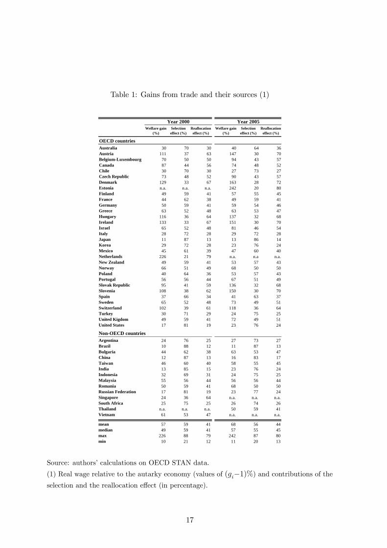
Table 1: Gains from trade and their sources (1)

Welfare gain(%)

Selectioneffect (%)

Reallocationeffect (%)

Welfare gain(%)

Selectioneffect (%)

Reallocationeffect (%)

OECD countriesAustralia 30 70 30 40 64 36Austria 111 37 63 147 30 70Belgium­Luxembourg 70 50 50 94 43 57Canada 87 44 56 74 48 52Chile 30 70 30 27 73 27Czech Republic 73 48 52 90 43 57Denmark 129 33 67 163 28 72Estonia n.a. n.a. n.a. 242 20 80Finland 49 59 41 57 55 45France 44 62 38 49 59 41Germany 50 59 41 59 54 46Greece 63 52 48 63 53 47Hungary 116 36 64 137 32 68Ireland 133 33 67 151 30 70Israel 65 52 48 81 46 54Italy 28 72 28 29 72 28Japan 11 87 13 13 86 14Korea 29 72 28 23 76 24Mexico 45 61 39 47 60 40Netherlands 226 21 79 n.a. n.a n.a.New Zealand 49 59 41 53 57 43Norway 66 51 49 68 50 50Poland 40 64 36 53 57 43Portugal 56 56 44 67 51 49Slovak Republic 95 41 59 136 32 68Slovenia 108 38 62 150 30 70Spain 37 66 34 41 63 37Sweden 65 52 48 73 49 51Switzerland 102 39 61 118 36 64Turkey 30 71 29 24 75 25United Kigdom 49 59 41 72 49 51United States 17 81 19 23 76 24

Non­OECD countriesArgentina 24 76 25 27 73 27Brazil 10 88 12 11 87 13Bulgaria 44 62 38 63 53 47China 12 87 13 16 83 17Taiwan 46 60 40 58 55 45India 13 85 15 23 76 24Indonesia 32 69 31 24 75 25Malaysia 55 56 44 56 56 44Romania 50 59 41 68 50 50Russian Federation 17 81 19 23 77 24Singapore 24 36 64 n.a. n.a. n.a.South Africa 25 75 25 26 74 26Thailand n.a. n.a. n.a. 50 59 41Vietnam 61 53 47 n.a. n.a. n.a.

mean 57 59 41 68 56 44median 49 59 41 57 55 45max 226 88 79 242 87 80min 10 21 12 11 20 13

Year 2000 Year 2005

Source: authors’calculations on OECD STAN data.

(1) Real wage relative to the autarky economy (values of (gi−1)%) and contributions of the

selection and the reallocation effect (in percentage).

17

around 55 per cent in 2005). It is worth noting that, unlike the gains from trade, the two

shares remain unchanged irrespectively of the exact value of θ and β. Unsurprisingly,

the reallocation effect is more important in small open economies, such as Denmark,

Estonia, Ireland, the Netherlands, Slovenia, Singapore, Thailand, and Vietnam. For

these countries, the share of the welfare gains pertaining to the reallocation effect is

above 70 percent in at least one year. On the other hand, for large and relatively more

closed countries, it is the selection effect that it is dominant. For instance, among the

OECD economies, only the United States and Japan record a share of the welfare gains

pertaining to the selection effect above 80 percent in at least one year. Among non-

OECD economies, only the BRIC countries (Brazil, Russia, India, and China) show

the same record as the United States and Japan.

5 Conclusion

This paper provides a deconstruction of the sources of the welfare gains from trade in a

Ricardian model. Under general distributions of industry effi ciencies, welfare gains arise

from two distinct sources. The former is an effect due to the selection of industries that

survive international competition. The latter is related to the reallocation of workers

away from the industries that shut down, as well as from those selling only in the

domestic market, to the industries that start servicing the foreign market. If industry

effi ciencies are Fréchet distributed, so that the model becomes one of the quantitative

trade models of Arkolakis, Costinot and Rodríguez-Clare (2012), these two effects can

be easily measured.

Our results also show that the share of the welfare gains due the reallocation

effect is larger, the larger is the welfare gain. Thus, countries that can potentially gain

more from trade – i.e. small open economies that are close to large, rich, and less

effi cient markets – would gain mostly from the reallocation effect. Therefore, to fully

reap the benefits from international trade, they must be ready to favor the reallocation

of resources towards exporting industries, for example supporting workers’education

and training.

The key insight from our analysis, however, is that quantitative trade models

seem to be useful not only in order to assess the overall welfare gains, but also to

properly measure their sources – an issue that deserves to be further explored in

future studies tackling other models in this class. The route taken in this paper of

using quantitative trade models to measure not only the overall welfare gains from

trade, but also the contribution of their sources, appears to be a promising area for

theoretical and empirical research.

18

Appendix

A Welfare decomposition with many countries

In order to prove equation (13), let us start by generalizing the resource constraint (9)

to a context with more than just two countries. As in the two-country case, we still

have: qi (j) = 0, if j ∈ Oi,z and qi (j) = ci (j) /β, if j ∈ Oi,d. Now consider the set of

industries of country i that export in (and only) the countries n, h, ..., and k, for any

n, h, ..., k ∈ 1, ..., N \ i, and denote this set by On,h,...,ki,e ;25 the resource constraint

for these industries becomes:

qi (j) =1

β[ci (j) + cn (j) dni + ch (j) dhi + ...+ ck (j) dki] .

Solving the resource constraint for the number of workers in industry j, we obtain:

Li (j) =

0 if j ∈ Oi,z

zσ−1i (j) ·(wipi

)β(1−σ)Li if j ∈ Oi,d

zσ−1i (j) ·(wipi

)β(1−σ)Li · (1 + kni + khi + ...+ kki) if j ∈ On,h,...,k

i,e

, (22)

where the terms kli are defined as in equation (11), for any destination market l.

Note that the sets Oi,z, Oi,d, On,h,...,ki,e (for any n, h, ..., k as above) form a par-

tition of the set of tradable goods. By aggregating across industries both sides of

equation (22), we obtain the following:(wipi

)β(σ−1)= λi,d·E

(Zσ−1i,d

)+...+λi,e;n,h,...,k·(1 + kni + khi + ...+ kki)·E

(Zσ−1i,e;n,h,...,k

)+...

(23)

where λi,d is the probability that an industry of country i survives international compe-

tition and serves only the domestic market (i.e. λi,d = Pr(Zi ∈ Oi,d)); λi,e;n,h,...,k is the

probability that an industry of country i exports in (and only) countries n, h, ..., and

k (i.e. λi,e;n,h,...,k = Pr(Zi ∈ On,h,...,ki,e )); Zi,e;n,h,...,k is the distribution of the effi ciencies

of these industries (i.e. Zi,e;n,h,...,k = Zi|Zi ∈ On,h,...,ki,e ). Considering that:

λi,o · E(Zσ−1i,o

)= λi,d · E

(Zσ−1i,d

)+ ...+ λi,e;n,h,...,k · E

(Zσ−1i,e;n,h,...,k

)+ ... ,

25The analytical definition of On,h,...,ki,e is as follows: this set includes all the industries that export

in countries n, h, ..., and k, i.e. those for which zi (j) /ci > zl (j) dli/cl, for l = n, h, ..., k; and excludes

those that export in countries different from n, h, ..., and k, i.e. those for which zi (j) /ci < zl (j) dli/cl

for l 6= n, h, ..., k.

19

we can conveniently rearrange the right-hand side of equation (23) into the sum of

two terms, given by equations (14) and (15). By taking the 1/β (σ − 1) power of both

sides, we finally obtain equation (13).

20

References

[1] Alvarez F. and R. Lucas (2007), "General Equilibrium Analysis of the Eaton-

Kortum Model of International Trade," Journal of Monetary Economics, Vol. 54,

pp. 1726-1768.

[2] Arkolakis C., A. Costinot and A. Rodríguez-Clare (2012), "New Trade Models,

Same Old Gains?," American Economic Review, Vol. 102, pp. 94-13.

[3] Arkolakis C., A. Costinot, D. Donaldson and A. Rodríguez-Clare (2012), "The

Elusive Pro-Competitive Effects of Trade," mimeo, Yale, MIT and University of

California, Berkeley.

[4] Arkolakis C., S. Demidova, P. Klenow and A. Rodríguez-Clare (2008), "Endoge-

nous Variety and the Gains from Trade," American Economic Review, Vol. 98,

pp. 444-50.

[5] Bernard A., Jensen J.B., Redding S.J., Schott P.K. (2007), "Firms in International

Trade," Journal of Economic Perspectives, Vol. 21, pp. 105-130.

[6] Bernard A., J. Eaton, B. Jensen and S. Kortum (2003), "Plants and Productivity

in International Trade," American Economic Review, Vol. 93, pp. 1268-1290.

[7] Bolatto S. (2013), "Trade across Countries and Manufacturing Sectors in a Ricar-

dian World," mimeo, Università di Torino.

[8] Broda C. and D. Weinstein (2006), "Globalization and the Gains from Variety,"

The Quarterly Journal of Economics, Vol. 121, pp. 541-585.

[9] Caballero R., T. Hoshi and A. Kashyap (2008), "Zombie Lending and Depressed

Restructuring in Japan," American Economic Review, Vol. 98, pp. 1943-1977.

[10] Chaney T. (2008), "Distorted Gravity: the Intensive and Extensive Margins of

International Trade," American Economic Review, Vol. 98, pp. 1707-21.

[11] Costinot A., D. Donaldson and I. Komunjer (2012), "What Goods Do Countries

Trade? A Quantitative Exploration of Ricardo’s Ideas," Review of Economic Stud-

ies, Vol. 79, pp. 581-608.

[12] Demidova S. and A. Rodríguez-Clare (2009), "Trade Policy under Firm-Level Het-

erogeneity in a Small Economy," Journal of International Economics, Vol. 78, pp.

100-112.

21

[13] Di Nino V., B. Eichengreen and M. Sbracia (2013), "Exchange Rates in a General

Equilibrium Model of Trade without Money," mimeo, Banca d’Italia and Univer-

sity of California, Berkeley.

[14] Eaton, J. and S. Kortum (2002), "Technology, Geography and Trade," Economet-

rica, Vol. 70, pp. 1741-1779.

[15] Eaton J. and S. Kortum (2009), "Technology in the Global Economy: a Framework

for Quantitative Analysis," mimeo, Princeton University Press (forthcoming).

[16] Eaton J., S. Kortum and F. Kramarz (2011), "An Anatomy of International Trade:

Evidence from French Firms," Econometrica, Vol. 79, pp. 1453-1498.

[17] Feenstra R.C. (1994), "New Product Varieties and the Measurement of Interna-

tional Prices," American Economic Review, Vol. 84, pp. 157-177.

[18] Feenstra R.C. (2010), "Measuring the Gains from Trade under Monopolistic Com-

petition," Canadian Journal of Economics, Vol. 43, pp. 1-28.

[19] Finicelli A., P. Pagano and M. Sbracia (2013a), "Ricardian Selection," Journal of

International Economics, Vol. 89, pp. 96-109.

[20] Finicelli A., P. Pagano and M. Sbracia (2013b), "Trade-Revealed TFP," mimeo,

Banca d’Italia.

[21] Goldberg P., A. Khandelwal, N. Pavcnik and P. Topalova (2010), "Trade Liber-

alization and New Imported Inputs," American Economic Review, Vol. 99, pp.

494-500.

[22] Kortum S. (1997), "Research, Patenting, and Technological Change," Economet-

rica, Vol. 65 (6), pp. 1389-1420.

[23] Krugman P. (1980), "Scale Economies, Product Differentiation, and the Pattern

of Trade," American Economic Review, Vol. 70, pp. 950-959.

[24] Levchenko A.A., Zhang J. (2013), "The Evolution of Comparative Advantage:

Measurement and Welfare Implications," mimeo, University of Michigan.

[25] Melitz M. (2003), "The Impact of Trade on Intra-Industry Reallocations and Ag-

gregate Industry Productivity," Econometrica, Vol. 71, pp. 1695-1725.

[26] Melitz M. and S.J. Redding (2013), "New Trade Models, New Welfare Implica-

tions," NBER Working Paper, No. 18919.

22

[27] Melitz M. and S.J. Redding (2014), "Missing Gains from Trade?," American Eco-

nomic Review, forthcoming.

[28] Pavcnik N. (2002), "Trade Liberalization, Exit, and Productivity Improvements:

Evidence from Chilean Plants," Review of Economic Studies, Vol. 69, pp. 245-276.

[29] Ravikumar B. and M. Waugh (2009), "On the Cross-country Distribution of Wel-

fare Gains from Trade," mimeo, New York University.

[30] Simonovska I. and M. Waugh (2014a), "Different Trade Models, Different Trade

Elasticities," mimeo, New York University and University of California, Davis.

[31] Simonovska I. and M. Waugh (2014b), "The Elasticity of Trade: Estimates and

Evidence," Journal of International Economics, Vol. 92, pp. 34-50.

23