radar techniques for identifying precipitation type and estimating

Radar techniques for identifying precipitation type and estimating quantity of precipitation

Document of COST Action 717, WG 1

Task WG 1-2

Milan Šálek1, Jean-Luc Cheze2, Jan Handwerker3, Laurent Delobbe4, Remko Uijlenhoet5

1Czech Hydrometeorological Institute 2Météo France

3Institut für Meteorologie und Klimaforschung, FZ Karlsruhe 4Royal Meteorological Institute of Belgium

5Wageningen University

July 2004

1 Background The early era of weather radar research was accompanied by enthusiasm about the capability of measuring precipitation by radar systems. Since its birth, weather radar has been offering prompt overviews of precipitating clouds, their structure and development. Considerable effort was taken in the second half of 20th century to use more quantitative information that could be used in other hydrometeorological information systems, especially in hydrological modelling and numerical weather prediction (NWP). In the beginning, expectations about the accuracy of radar measurement of precipitation were high but nowadays it is apparent that weather radar measurement is often accompanied with non-negligible and sometimes large errors; hence the radar can be referred as a semi-quantitative measurement device (Joss et al, 1998). The errors stem from the nature of the measurement and are highly influenced by the meteorological conditions, especially by precipitation processes and by the size distribution of precipitation particles. Nevertheless, radar still provides very useful information; its real-time coverage and prompt availability of the data are particularly valuable.

Since rainfall constitutes the main source of water for the terrestrial hydrological processes, accurate measurement and prediction of the spatial and temporal distribution of rainfall is a basic issue in hydrology. As a result of the gradual development of radar technology over the past 50 years, ground-based weather radar is now finally becoming a tool for quantitative rainfall measurement instead of merely for qualitative rainfall estimation. Potential areas of application of ground-based weather radar systems in operational hydrology include storm hazard assessment and flood forecasting, warning, and control (Collier, 1989). The current attention for land surface hydrological processes in the climate system has stimulated research into the spatial and temporal variability of rainfall as well. A potential area of application of ground-based weather radar in this context is the validation and verification of sub-grid rainfall parameterizations for atmospheric mesoscale models and general circulation models.

Regarding the quantitative precipitation estimation (QPE), there is an extensive literature because QPE was an issue since the first radar meteorological observations and it is still one of the very important ones, and because it has not been solved satisfactorily. To get a good

Radar techniques for identifying precipitation type and estimating quantity of precipitation 1

overview of QPE issues we recommend looking at Zawadzki (1984) and Joss and Waldvogel (1990). Although radar technology has improved since that time (most radars have a Doppler facility nowadays), the descriptions of the fundamental physical mechanisms are still valid.

For an overview of the state of the art of radar data processing, see the final report of the COST 75 action (Collier, 2001) and the recently printed textbook of Meischner et al. (2003). These references can also be used to find further literature about several error correction procedures.

A good scan strategy and appropriate data processing may improve data quality in every application. However, hydrological applications have often to utilize radar data that are gathered primarily for another purpose, e.g. qualitative nowcasting. Here, we describe the steps that may improve data quality during the measurement and explain the errors which can be expected if the measuring procedure is not specifically designed for the hydrological applications.

One of the aims of COST Action 717 is to evaluate the potential of weather radar to provide hydrological simulation and forecasting systems with information regarding primarily quantitative precipitation estimation. The quality of the estimates is related to the precipitation type and thus the quantitative precipitation estimate should be accompanied with information on the precipitation type, either derived only from the radar measurement or provided by other information sources (measurement networks, NWP models).

While the principle of radar precipitation estimation are relatively well known and routinely used in many operational systems, the classification of precipitation type by radar is not so widespread and is generally done with dual polarization (or dual wavelength) methods which are still limited mainly to research experiments (with some exceptions). However, some nowcasting systems provide and use the categorization of precipitation type with the help of other information sources, especially surface and/or upper air observations or NWP models.

This text aims to provide an introduction to the state of the art of radar quantitative precipitation estimation for hydrological applications and a brief review of the techniques of radar precipitation measurement and methods for the identification of the precipitation type. The latter topic will be a little enlarged to mention the importance of multisource (multisensor) methods that integrate radar measurements and other meteorological data. Quantitative precipitation forecasting (QPF) is beyond the scope of this text and is covered in a review already published (Mecklenburg et al., 2002).

2 Principles of radar measurement of precipitation Radar measurement of precipitation is a complex issue and only the main principles will be presented here. For a more detailed treatment see for instance, Doviak and Zrnic (1993), Collier (1996), Sauvageot (1992), Bringi and Chandrasekhar (2001) or Rinehart (1997).

Weather radar obtains volume information by rotating an antenna with a variable vertical angle according to a predefined scanning strategy. The radar antenna emits a short pulse of electromagnetic radiation in a known direction and a small fraction of this energy is reflected by targets (meteorological and non-meteorological) back to the radar antenna. The back-scattered mean power rP received by the radar is proportional to the reflectivity factor Z (provided the scattering particles are considerably – by order of magnitude – smaller then the

wavelength and are of spherical shape), and to the factor 2

2

22

21

+−

=mmK , which is a function


of complex refractivity index m and thus dielectric constant of the target. The received power is also proportional to the radar constant C (including e.g. the emitted power) and inversely proportional to the square of the target distance r2 and the square of the one-way atmospheric attenuation LAtm. The simplified form of the radar equation is then (e.g. Joss and Waldvogel, 1990):

2

2

2 rZK

LCPAtm

r = (1)

The radar constant reflects the radar properties as the emitted power, pulse length, 3-dB beam shape, antenna gain and attenuation of the radar hardware including the attenuation of amplifiers within the receiver. As the radar constant must be determined, the parameters mentioned above have to be known. Some of these values are assumed (hoped) to be constant and thus are measured once by the manufacturer. The distortion of beam by the radome is mostly neglected and some of these values are measured and/or calibrated regularly.

Since the dielectric constant changes with the particles’ phase, the 2K value for water is approx. 0.93 whilst its value for ice is about 0.18; the difference should be taken into account if radar measures precipitation where the solid phase of precipitation is important (see section 4.2.4).

Z (mm6 m-3), the radar reflectivity factor, is hereafter simply referred to as radar reflectivity. All radar properties are contained in C, and all raindrop properties in 2K and Z. Z is related to the size distribution of the raindrops in the radar sample volume according to (e.g. Battan, 1973)

( )∫∞

=0

6 ,dDDNDZ V (2)

where (the subscript V standing for volume) represents the mean number of raindrops with equivalent spherical diameters between D and

( )dDDNV

dDD + (mm) present per unit volume of air1. The corresponding units of ( )DNV are mm-1 m-3. Hence, although Z is called the radar reflectivity factor, it is a purely meteorological quantity that is independent of any radar property. Because in practice the variations in radar reflectivity may span several orders of magnitude, it is often convenient to use a logarithmic scale. The logarithmic radar reflectivity is defined as and is expressed in units of dBZ (e.g. Battan, 1973). Zlog10

However, the radar equation is accurate only under specific assumptions (e.g. physical properties of the target, beam filling with the randomly scattered precipitation particles, uniform factor Z through the sample volume, etc., see Collier, 1996) that often do not occur in the real environment. Especially the assumption that hydrometeors are water spheroids with diameter inside the Rayleigh scattering region is often far from the reality. Therefore a quantity called the effective (or equivalent) radar reflectivity Ze is used. The quantity Ze is defined as the summation per unit volume of the sixth power of the diameter of spherical water drops in the Rayleigh scattering region, which would backscatter the same power as the measured reflectivity (Collier, 1996).

1 The raindrop diameter integration limits have been assumed to be zero and infinity, respectively. In other words, the effects of truncation of the raindrop size distribution (e.g. Ulbrich, 1985) have been disregarded.


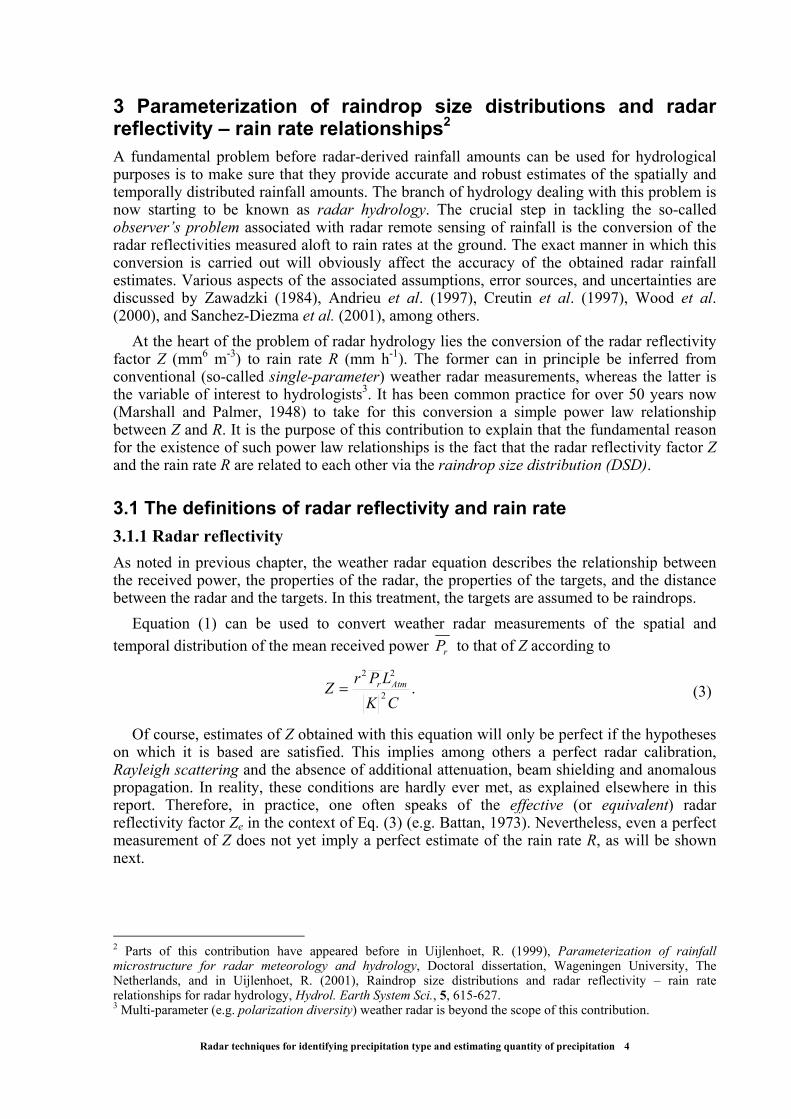
3 Parameterization of raindrop size distributions and radar reflectivity – rain rate relationships2

A fundamental problem before radar-derived rainfall amounts can be used for hydrological purposes is to make sure that they provide accurate and robust estimates of the spatially and temporally distributed rainfall amounts. The branch of hydrology dealing with this problem is now starting to be known as radar hydrology. The crucial step in tackling the so-called observer’s problem associated with radar remote sensing of rainfall is the conversion of the radar reflectivities measured aloft to rain rates at the ground. The exact manner in which this conversion is carried out will obviously affect the accuracy of the obtained radar rainfall estimates. Various aspects of the associated assumptions, error sources, and uncertainties are discussed by Zawadzki (1984), Andrieu et al. (1997), Creutin et al. (1997), Wood et al. (2000), and Sanchez-Diezma et al. (2001), among others.

At the heart of the problem of radar hydrology lies the conversion of the radar reflectivity factor Z (mm6 m-3) to rain rate R (mm h-1). The former can in principle be inferred from conventional (so-called single-parameter) weather radar measurements, whereas the latter is the variable of interest to hydrologists3. It has been common practice for over 50 years now (Marshall and Palmer, 1948) to take for this conversion a simple power law relationship between Z and R. It is the purpose of this contribution to explain that the fundamental reason for the existence of such power law relationships is the fact that the radar reflectivity factor Z and the rain rate R are related to each other via the raindrop size distribution (DSD).

3.1 The definitions of radar reflectivity and rain rate 3.1.1 Radar reflectivity As noted in previous chapter, the weather radar equation describes the relationship between the received power, the properties of the radar, the properties of the targets, and the distance between the radar and the targets. In this treatment, the targets are assumed to be raindrops.

Equation (1) can be used to convert weather radar measurements of the spatial and temporal distribution of the mean received power rP to that of Z according to

.2

22

CKLPrZ Atmr= (3)

Of course, estimates of Z obtained with this equation will only be perfect if the hypotheses on which it is based are satisfied. This implies among others a perfect radar calibration, Rayleigh scattering and the absence of additional attenuation, beam shielding and anomalous propagation. In reality, these conditions are hardly ever met, as explained elsewhere in this report. Therefore, in practice, one often speaks of the effective (or equivalent) radar reflectivity factor Ze in the context of Eq. (3) (e.g. Battan, 1973). Nevertheless, even a perfect measurement of Z does not yet imply a perfect estimate of the rain rate R, as will be shown next.

2 Parts of this contribution have appeared before in Uijlenhoet, R. (1999), Parameterization of rainfall microstructure for radar meteorology and hydrology, Doctoral dissertation, Wageningen University, The Netherlands, and in Uijlenhoet, R. (2001), Raindrop size distributions and radar reflectivity – rain rate relationships for radar hydrology, Hydrol. Earth System Sci., 5, 615-627. 3 Multi-parameter (e.g. polarization diversity) weather radar is beyond the scope of this contribution.


3.1.2 Rain rate If the effects of wind (notably updrafts and downdrafts), turbulence, and raindrop interaction are neglected, the (stationary) rain rate R (in mm h-1) is related to the raindrop size distribution according to ( )DNV

( ) ( )∫∞

−×=0

34 ,106 dDDNDvDR Vπ (4)

where represents the functional relationship between the raindrop terminal fall speed in still air v (m s

( )Dv-1) and the equivalent spherical raindrop diameter D (mm). The simplest and

most widely used form of the -relationship is the power law ( )Dv

( ) .γcDDv = (5)

Atlas and Ulbrich (1977) demonstrated that Eq. (5) with 778.3=c (if v is expressed in m s-1 and D in mm) and 67.0=γ provides a close fit to the data of Gunn and Kinzer (1949) in the range mm (the diameter interval contributing most to rain rate). Although more sophisticated relationships have been proposed in the literature (e.g. Atlas et al., 1973), the power law form for the -relationship is the only functional form that is consistent with power law relationships between rainfall-related variables, notably between Z and R (Uijlenhoet, 1999).

0.55.0 ≤≤ D

( )Dv

A comparison of Eq. (4) with Eq. (2) demonstrates that it is the raindrop size distribution (and to a lesser extent also the ( )DNV ( )Dv -relationship) that ties Z to R. This is the reason

why the analysis of raindrop size distributions and the associated Z–R relationships is of interest to hydrologists (Smith and Krajewski, 1993; Steiner et al., 2004). In hydrological applications, it is clearly not the spatial and temporal distribution of Z that is of interest, but rather that of the rain rate R. A complicating factor in this respect is the fact that the measurements of Z are made aloft, whereas estimates of R are generally needed at ground level. The difference between the value of Z aloft and that at the ground is determined by the vertical profile of reflectivity. Only at ranges close to the radar, where the height of the radar beam above the ground is small, can this factor be neglected. Even then, the time it takes the raindrops to fall from the radar sample volume down to the ground should often be taken into account.

Even if weather radar were to provide perfect measurements of the spatial and temporal distributions of Z at ground level, the radar rainfall measurement problem would not be solved completely. First of all, the relationship between the radar reflectivity factor Z and the rain rate R is generally not a unique relationship. Secondly, even if it were unique, it would generally be unknown. This fundamental uncertainty in the Z–R relationship provides a lower limit to the overall uncertainty associated with radar rainfall estimation. In the absence of any other error source affecting the radar estimation of Z, the rainfall measurement problem for single-parameter weather radar reduces therefore to optimally using the information Z is supplying about the raindrop size distribution for the estimation of R.

3.2 Empirical radar reflectivity – rain rate relationships On the basis of measurements of raindrop size distributions at the ground and an assumption about the -relationship (such as Eq. (5)), it is possible to derive Z–R relationships (via regression analysis). There exists overwhelming empirical evidence (e.g. Battan, 1973) that such relationships generally follow power laws of the form

( )Dv


,baRZ = (6)

where a and b are coefficients that may vary from one location to the next and from one season to the next, but that are independent of R itself. These coefficients will in some sense reflect the climatological character of a particular location or season, or more specifically the type of rainfall (e.g. stratiform, convective, orographic) for which they are derived.

Battan’s (1973) standard treatise on radar meteorology quotes a list of 69 of such empirical power law Z–R relationships derived for different climatic settings in various parts of the world (his Table 7.1, p. 90-92). Figure 1a provides all these relationships in one single plot. For reference, the linear Z–R relationship proposed by List (1988) for equilibrium rainfall conditions (which have been observed during ‘steady tropical rain’) is included as well. Figure 1b shows that, although there is an appreciable variability in the coefficients of these Z–R relationships associated with differences in rainfall climatologies, there seems to be a well-defined envelope comprising most relationships. A naive approach (taking the geometric mean of the individual prefactors a and the arithmetic mean of the exponents b – corresponding to averaging the linear – relationships) leads to the mean power law relationship

Zlog Rlog

.238 50.1RZ = (7)

Figure 1b compares this relationship with the so-called Marshall-Palmer Z–R relationship, 6.1200RZ = (8)

(Marshall and Palmer, 1948; Marshall et al., 1955). The correspondence is close, particularly for rain rates between 1 and 50 mm h-1. This may be an explanation for the success of Eq. (8) for many different types of rainfall in many parts of the world, even though the Marshall-Palmer Z–R relationship is based on measurements of raindrop size distributions in Montreal, Canada, mainly in stratiform precipitation.

The question is whether the coefficients a and b of the power law Z–R relationships are systematically different for different types of rainfall. Figure 2 shows a plot of b versus a for Battan's 69 Z–R relationships. On the basis of the remarks given by Battan (in his Table 7.1), it is possible to associate 25 of these Z–R relationships unambiguously with a particular type of rainfall. Using the same stratification as Ulbrich (1983), 4 of the relationships can be associated with ‘orographic’ rainfall, 5 with ‘thunderstorm’ rainfall, 10 with ‘widespread’ or ‘stratiform’ rainfall, and 6 with ‘showers’. The remaining 44 relationships cannot be unambiguously associated with a particular type of rainfall, either because they correspond to mixtures of different rainfall types or because the rainfall type is not specified at all. Figure 2 provides some indication that the orographic and thunderstorm Z–R relationships form coherent groups in the -phase space. On average, orographic rainfall tends to be associated with smaller prefactors and larger exponents, whereas for thunderstorm rainfall the opposite seems to be the case. For the Z–R relationships associated with the other rainfall types, it is less obvious to make unambiguous statements about their positions in the

( ba, )

( )ba, -phase space. A physical interpretation of the coefficients a and b in terms of the parameters of the corresponding raindrop size distributions may help to explain their variability.


Figure 1: (a) The 69 power law Z–R relationships quoted by Battan (1973; p. 90-92), including five deviating relationships (dashed lines), four of which have prefactors a significantly smaller than 100 and one of which has an exponent b as high as 2.87. The bold line indicates the linear relationship (List, 1988). (b) The mean of Battan’s relationships, (bold solid line), the reference relationship

(Marshall et al., 1955; bold dashed line), and the envelope (thin solid lines) of 64 (the thin solid lines in (a)) of Battan’s 69 Z–R relationships (Uijlenhoet, 1999, 2001).

baRZ =

RZ 742=50.1238RZ =

6.1200RZ =


Figure 2: The coefficients a and b of the 69 power law Z–R relationships (with Z expressed in mmbaRZ = 6 m-3 and R in mm h-1) quoted by Battan (1973), stratified according to rainfall type: orographic (circles); thunderstorm (triangles); widespread/stratiform (stars); showers (squares); no unambiguous identification possible (dots). The dashed lines correspond to the reference relationship (Marshall et al., 1955); the dash-dotted lines correspond to Marshall and Palmer’s (1948) relationship , which almost equals the mean of Battan’s relationships, (Uijlenhoet, 1999, 2001).

6.1200RZ =50.1237RZ =

50.1238RZ =

3.3 Parameterization of the raindrop size distribution 3.3.1 The exponential raindrop size distribution Since, according to Eqs. (2) and (4), both Z and R are related to the raindrop size distribution

, it should be possible to express a and b as functions of the parameters of ( )DNV ( )DNV . Although many different parameterizations for ( )DNV have been proposed in the literature, notably the gamma (Ulbrich, 1983) and lognormal (Feingold and Levin, 1986) forms, the exponential raindrop size distribution introduced by Marshall and Palmer (1948) has found the widest application. There exists empirical evidence showing that averaged raindrop size distributions indeed generally tend to the exponential form (Joss and Gori, 1978; Ulbrich and Atlas, 1998). Note that the exponential parameterization will be used here merely as an example of a family of raindrop size distributions. A general approach to deriving Z–R relationships, independent of any a priori assumption regarding the exact functional form of the raindrop size distribution, is presented later.


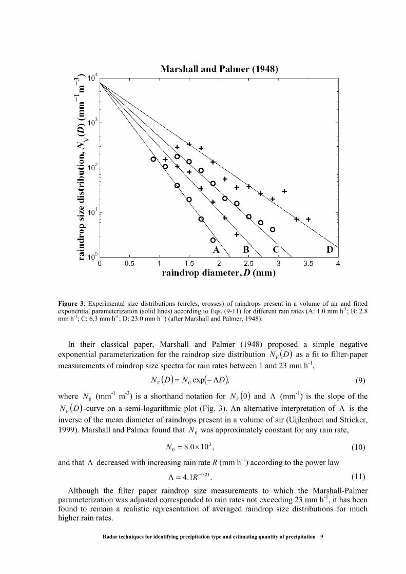
Figure 3: Experimental size distributions (circles, crosses) of raindrops present in a volume of air and fitted exponential parameterization (solid lines) according to Eqs. (9-11) for different rain rates (A: 1.0 mm h-1; B: 2.8 mm h-1; C: 6.3 mm h-1; D: 23.0 mm h-1) (after Marshall and Palmer, 1948).

In their classical paper, Marshall and Palmer (1948) proposed a simple negative

exponential parameterization for the raindrop size distribution ( )DNV as a fit to filter-paper measurements of raindrop size spectra for rain rates between 1 and 23 mm h-1,

( ) ( ),exp0 DNDNV Λ−= (9)

where (mm0N -1 m-3) is a shorthand notation for ( )0VN and Λ (mm-1) is the slope of the -curve on a semi-logarithmic plot (Fig. 3). An alternative interpretation of ( )DNV Λ is the

inverse of the mean diameter of raindrops present in a volume of air (Uijlenhoet and Stricker, 1999). Marshall and Palmer found that was approximately constant for any rain rate, 0N

,100.8 30 ×=N (10)

and that decreased with increasing rain rate R (mm hΛ -1) according to the power law

.1.4 21.0−=Λ R (11)

Although the filter paper raindrop size measurements to which the Marshall-Palmer parameterization was adjusted corresponded to rain rates not exceeding 23 mm h-1, it has been found to remain a realistic representation of averaged raindrop size distributions for much higher rain rates.


3.3.2 Scaling law for the raindrop size distribution Sempere Torres et al. (1994; 1998) have demonstrated that many previously proposed parameterizations for the raindrop size distribution are special cases of a general formulation, which takes the form of a scaling law4. In this formulation, the raindrop size distribution depends both on the raindrop diameter (D) and on the value of a so-called reference variable, commonly taken to be the rain rate (R). The generality of this formulation stems from the fact that it is no longer necessary to impose an a priori functional form for the raindrop size distribution. Moreover, it naturally leads to the ubiquitous power law relationships between rainfall integral parameters, notably that between the radar reflectivity factor (Z) and R.

According to the scaling law formalism, raindrop size distributions can be parameterized as (Sempere Torres et al., 1994; 1998)

)/(),( βα RDgRRDNV = , (12)

where (mm( RDNV , ) -1 m-3) is the raindrop size distribution as a function of the (equivalent spherical) raindrop diameter D (mm) and the rain rate R (mm h-1), α and β are (dimensionless) scaling exponents, and ( )xg is the general raindrop size distribution as a function of the scaled raindrop diameter . In agreement with common practice, R is used as the reference variable in Eq. (12), although any other rainfall integral variable could serve as such (notably Z). According to this formulation, the values of

βRDx /=

α and β and the form and dimensions of depend on the choice of the reference variable, but do not bear any functional dependence on its value.

( )xg

The importance of the scaling law formalism for radar hydrology stems from the fact that it allows an interpretation of the coefficients of Z–R relationships in terms of the values of the scaling exponents and the shape of the general raindrop size distribution. Substituting Eq. (12) into the definition of Z in terms of the raindrop size distribution, Eq. (2), leads to a power law Z–R relationship, Eq. (6), with

∫∞

=0

6 )( dxxgxa , (13)

and βα 7+=b (14)

(Uijlenhoet, 1999, 2001). Hence, the prefactors of power law Z–R relationships are entirely determined by the shape of the general raindrop size distribution (they are in fact its 6th moment), whereas a linear combination of the values of the scaling exponents completely determines the exponents of such power law Z–R relationships.

In a similar manner, the scaling law formalism leads to power law relationships between any other pair of rainfall integral variables. In particular, substituting Eq. (12) into the definition of R in terms of the raindrop size distribution, Eq. (4), and assuming a power law raindrop terminal fall speed parameterization, Eq. (5), leads to the self-consistency constraints

1)(1060

34 =× ∫∞

+− dxxgxc γπ , (15)

and 4 Recently proposed approaches to normalizing raindrop size distributions using two reference variables (Testud et al., 2001; Illingworth and Blackman, 2002; Lee et al., 2004) are beyond the scope of this contribution.


( ) 14 =++ βγα (16)

(Sempere Torres et al., 1994). Hence, ( )xg must satisfy an integral equation (which reduces its degrees of freedom by one) and there is only one free scaling exponent. Substitution of the self-consistency constraint on the scaling exponents, Eq. (16), into the definition of b in terms of those scaling exponents, Eq. (14), yields

( )βγ−+= 31b (17)

in terms of the scaling exponent β , or an equivalent expression in terms of the scaling exponent α (Uijlenhoet, 1999, 2001). For 67.0=γ (Atlas and Ulbrich, 1977), Eq. (17) reduces to β33.21+=b . Hence, the exponents of power law Z–R relationships can be expressed explicitly in terms of both scaling exponents [which are related to each other via the self-consistency constraint Eq. (16)], independent of any assumption regarding the shape of the general raindrop size distribution. To obtain equivalent explicit expressions for the prefactors of power law Z–R relationships, however, a particular functional form for ( )xg needs to be assumed.

Consider an exponential parameterization for the general raindrop size distribution,

( ) ( ).exp xxg λκ −= (18)

In this general form, is not an admissible description of the general raindrop size distribution, because it does not satisfy the self-consistency constraint on , Eq. (15). Substitution of Eq. (18) into (15) yields a power law relationship of

( )xg( )xg

κ in terms of λ ,

( )[ ] ,4106 414 γλγπκ +−− +Γ×= c (19)

or an equivalent power law relationship of λ in terms of κ (Uijlenhoet, 1999, 2001). Equation (19) provides an explicit form of the self-consistency constraint on for the special case of an exponential parameterization. For the applied units, with and

( )xg778.3=c

67.0=γ (Atlas and Ulbrich, 1977), Eq. (19) reduces to . 67.450.9 λκ =

Hence, the self-consistency constraint on ( )xg reduces its number of free parameters by one. Since the exponential parameterization for ( )xg , Eq. (18), has only two parameters, namely κ and λ , the number of free parameters that remains, is only one (either κ or λ ). In the same manner as Eq. (16) describes a unique relationship between the scaling exponents α and β (depending only on the value of γ ), Eq. (19) describes a unique relationship between the parameters of the exponential form for the general raindrop size distribution (depending only on the values of c and γ ). As a result, for the special case of an exponential parameterization for , the total number of free parameters that is required to unambiguously describe the scaling law, Eq. (12), and any derived (power law) relationship between rainfall-related variables (notably Z–R relationships) is two: on the one hand either

( )xg

α or β , and on the other hand either κ or λ (Sempere Torres et al., 1994; 1998). Note that relationships similar to Eq. (19) can be developed for any other functional form for the general raindrop size distribution, notably the gamma and lognormal parameterizations (Uijlenhoet, 1999; Uijlenhoet et al., 2003a,b).

A general expression for the prefactors of power law Z–R relationships for the special case of an exponential parameterization for ( )xg can be obtained by substituting Eq. (18) into (13). This yields


( ) .7 7−Γ= κλa (20)

To guarantee that a satisfies the self-consistency constraint on ( )xg , Eq. (19) needs to be substituted into Eq. (20). This yields a power law relationship of a in terms of λ ,

( ) ( )[ ] ( ).41067 314 γλγπ −−−− +Γ×Γ= ca (21)

This equation (or an equivalent power law relationship of a in terms of κ ) complements Eq. (17) and together they form an internally consistent pair of relationships for the estimation of the prefactors and exponents of power law Z–R relationships in terms of the parameters of the exponential raindrop size distribution. For the applied units, with and 778.3=c 67.0=γ (Atlas and Ulbrich, 1977), Eq. (21) reduces to . 33.231084.6 −×= λa

3.3.3 Comparison of the scaling law with the exponential raindrop size distribution It is of considerable interest to establish a link between the scaling law formalism and the traditional analytical parameterizations for the raindrop size distribution. For the special case of the exponential raindrop size distribution, this can be achieved through substituting Eq. (18) into (12). This yields

( ) ( ).exp, DRRRDNVβα λκ −−= (22)

A comparison with Eq. (9) shows that Eq. (22) reduces to the classical exponential parameterization for the raindrop size distribution if and 0N Λ depend on R according to the power laws

ακRN =0 (23)

and

.βλ −=Λ R (24)

As opposed to Eq. (9), Eq. (22) is an intrinsically self-consistent form of the exponential raindrop size distribution. This is because, as has been demonstrated above, only two of the four parameters ( λκβα ,,, ) that define ( )RDNV , according to Eq. (22) can actually be chosen freely. More concretely, the coefficients of the power law –R and 0N Λ –R relationships defined by Eqs. (23) and (24) cannot be chosen without restrictions, but have to satisfy the self-consistency constraints imposed by Eqs. (16) and (19).

Now consider Marshall and Palmer’s (1948) assumption of a constant independent of the rain rate R, Eq. (10). Equation (23) shows that this special case corresponds to

,100.8 30 ×=N

κ=0N , or equivalently 0=α . Substituting Atlas and Ulbrich’s (1977) values for c and γ (for the applied units: 778.3=c and 67.0=γ ) and Marshall and Palmer’s (1948) value for into the self-consistency relations Eqs. (16) and (19) yields for the 0N Λ –R relationship, Eq. (24), For the corresponding Z–R relationship, Eq. (6) with a according to Eq. (21) and b according to Eq. (17), the same substitution yields . Interestingly, the coefficients of this relationship are almost exactly the same as those of the mean of Battan’s 69 Z–R relationships, Eq. (7). Finally, direct substitution of Eqs. (9)-(11) in

.23.4 214.0−=Λ R50.1237RZ =


Eq. (2) yields an expression reported by Marshall and Palmer (1948) as well. ,296 47.1RZ =

These calculations show that the Marshall-Palmer Λ –R relationship, Eq. (11), is actually not fully consistent with Atlas and Ulbrich’s (1977) values for c and γ and with the Marshall-Palmer value for (at least not for diameter integration limits of 0 and ∞ ). More importantly, they also show that Eq. (8), although it is commonly known as the Marshall-Palmer Z–R relationship, is not consistent with the Marshall-Palmer parameterization for the raindrop size distribution, Eqs. (9)-(11).

0N

3.4 Raindrop size distributions from empirical radar reflectivity – rain rate relationships Equations (17) and (21) resolve the issue of relating the coefficients of power law Z–R relationships to the parameters of the raindrop size distribution. Equation (21) can be inverted to estimate λ [and κ via Eq. (19)] from given values of a, in much the same way as Eq. (17) can be inverted to estimate β [and α via Eq. (16)] from given values of b. This approach provides the opportunity to investigate the dependence of the parameters of the (self-consistent exponential) raindrop size distribution on the type of rainfall using the coefficients of the 69 power law Z–R relationships quoted by Battan (1973) that have been discussed before. Figure 4a presents the results for the coefficients of the corresponding Λ –R relationships (parameterized as with βλ −=Λ R Λ expressed in mm-1 and R in mm h-1), Fig. 4b for the coefficients of the corresponding –R relationships ( with in mm0N ακRN =0 0N -1 m-3 and R in mm h-1). Figure 4b clearly demonstrates that Marshall and Palmer’s (1948) assumption of a constant is too restrictive in practice. Although the mean value of 0N α seems to be close to zero (indicating a constant ), there is a significant amount of variability between different rainfall climatologies.

0N

Both in terms of the –R relationship and in terms of the –R relationship, orographic rainfall tends to be associated with larger prefactors and smaller exponents. For thunderstorm rainfall, the opposite seems to be the case (Table 1). Recall that

Λ 0N

Λ is the inverse of the mean diameter of raindrops present in a volume of air and that represents the concentration of the smallest raindrops, Eq. (9). Bearing this in mind, the observations indicate that, at a given rain rate, orographic rainfall would exhibit smaller mean raindrop sizes and larger concentrations, whereas thunderstorm rainfall would be associated with larger mean drop sizes and smaller concentrations. This is exactly what one would expect for these types of rainfall. Moreover, it provides an explanation for the differences between the coefficients of the Z–R relationships corresponding to these rainfall types (Table 1, Fig. 2).

0N


Figure 4: (a) The coefficients λ and β− of power law Λ –R relationships (with expressed in mm

βλ −=Λ R Λ-1 and R in mm h-1) for the 69 exponential raindrop size distributions consistent with Battan’s (1973) Z–R

relationships, stratified according to rainfall type: orographic (circles); thunderstorm (triangles); widespread/stratiform (stars); showers (squares); no unambiguous identification possible (dots). The dashed lines correspond to the relationship , consistent with (Marshall et al., 1955); the dash-dotted lines correspond to the relationship , consistent with (Marshall and Palmer, 1948). (b) Idem for the coefficients

258.055.4 −=Λ R 6.1200RZ =214.023.4 −=Λ R 50.1237RZ =

κ and α of the 69 corresponding power law –R 0N


relationships (with expressed in mmακRN =0 0N -1 m-3 and R in mm h-1). The dashed lines correspond to the

relationship , consistent with (Marshall et al., 1955); the dash-dotted

lines correspond to the relationship , consistent with (Marshall and Palmer, 1948).

203.040 1013.1 −×= RN 6.1200RZ =

30 1000.8 ×=N 50.1237RZ =

Table 1: Mean values of the parameters of the self-consistent exponential raindrop size distribution, Eq. (22), and the corresponding mean values of the Z–R coefficients, as derived from Battan’s (1973) 69 Z–R relationships, stratified according to rainfall type. The category ‘Rest’ contains all relationships for which an unambiguous identification of rainfall type is impossible, ‘nr.’ denotes the number of relationships in each category (Uijlenhoet, 1999).

Rainfall type nr. α β κ λ a b

Orographic 4 -0.219 0.261 2.02×105 8.44 47 1.61

Thunderstorm 5 0.136 0.185 3.44×103 3.53 361 1.43

Widespread/ stratiform

10 0.117 0.189 7.74×103 4.20 241 1.44

Showers 6 -0.499 0.321 7.32×103 4.15 248 1.75

Rest 44 0.057 0.202 7.85×103 4.21 240 1.47

All 69 0.005 0.213 9.63×103 4.40 216 1.50

The relationships presented in Table 1 for orographic, thunderstorm and

widespread/stratiform rainfall correspond quite closely to those provided by Battan (1973) as being ‘typical’ for these types of rainfall. Moreover, the entries under ‘All’ indicate that the Marshall-Palmer Z–R relationship, Eq. (8), and the Marshall-Palmer parameterization for the raindrop size distribution, Eqs. (9)-(11), are reasonable approximations for average conditions.

3.5 Summary and conclusions regarding the parametrizations of the raindrop size distributions Many previously proposed parameterizations for the raindrop size distribution are special cases of a general formulation, which takes the form of a scaling law. Using this scaling law framework for describing raindrop size distributions and their properties, it has been shown (1) that the definitions of Z and R naturally lead to power law Z–R relationships, and (2) how the coefficients of such relationships are related to the parameters of the raindrop size distribution.

Using the classical exponential family of raindrop size distributions as an example, the 69 empirical Z–R relationships quoted by Battan (1973) have been analyzed in the scaling law framework. The objective was to verify whether there exist any systematic differences in the coefficients of Z–R relationships and the corresponding parameters of the (exponential) raindrop size distribution between different rainfall types. It was found that, at a given rain rate, orographic rainfall tends to exhibit smaller mean raindrop sizes and larger concentrations, whereas thunderstorm rainfall tends to be associated with larger mean raindrop sizes and smaller concentrations, which is exactly what one would expect for these types of rainfall. This interpretation provided an explanation for the smaller values of the prefactors and the larger values of the exponents of the Z–R relationships reported for orographic rainfall as compared to those reported for thunderstorm rainfall. Finally, the Marshall-Palmer Z–R relationship and the Marshall-Palmer parameterization for the raindrop size distribution were found to be reasonable approximations for average conditions.


4 Errors of the single parameter radar precipitation estimates Quantitative precipitation estimates by radar have a number of errors that stem from the nature of this kind of measurement. The quantification of the errors in radar is difficult because there are several independent error sources. Their relative importance varies greatly with weather conditions, distance to the radar, scan strategy, temporal and spatial resolution, orography, data processing or amount and quality of maintenance the radar is given. This makes it impossible to give a number like “the accuracy of radar precipitation estimates is x%”.

Discussing error characteristics we have to distinguish between systematic and random errors. The latter ones are reducing with the increasing size of the area and the increasing duration of the integration. The former ones might be reduced by the use of so called “ground truth” data from rain gauge networks or by correction using vertical profiles of reflectivity (see section 4.2.2).

The quality of radar data is often assessed by comparing radar rainfall estimates to rain gauge measurements. For this comparison it is common to compare the measurement error of a gauge with that of a single radar value (mean rainfall accumulation of an areal element, usually of side length of several hundreds meters or several kilometers). These comparisons suffer mainly from the problem of rain gauge representativity (sampling problem). Short term comparisons on the basis of minutes, hours or even days show a significant scatter because the radar averages over an area of the order of 1 km2, whereas the rain gauge uses an area that is roughly 10 orders of magnitude smaller. Especially in convective precipitation, when very steep horizontal gradients of precipitation are observed, the information of the rain gauges can be misleading.

It must be stressed that radar and rain gauges are not competitive but complementary sensors. The best results are achieved by a combination of the information from both measurement systems. This improves not only the quality of the data, but it puts redundancy into the game, giving still some information on the precipitation when one of the two systems is malfunctioning.

The radar measurement errors may be classified into instrumental (or non-meteorological) errors and errors caused by changes in the meteorological conditions (meteorological errors) including the above mentioned drop size distribution.

Most of the discrepancies between ground-based measurements (such as from a dense network of rain gauges) and radar precipitation estimates are because the radar measures the precipitation in a relatively large sample volume at some height above the ground. The characteristics of precipitation, as e.g. liquid water content, can significantly change with height and hence the precipitation estimation aloft may not be representative of what the ground surface receives.

4.1 Non-meteorological errors of the single parameter radar precipitation estimates Non-meteorological errors are caused by beam propagation, clutter, radar hardware and overall data processing, which is not a simple task. The radar system must consistently cope with electrical power across twenty orders of magnitude. An example of the simplification whose effects are often neglected is the gaussian shape of the radar beam whose boundaries are artificially determined as a power by 3dB (50 %) less than the peak power; another example is the often neglected influence of side lobes in the vicinity of the radar.


4.1.1 Calibration of the radar Several parts of the radar parameters, e.g. antenna gain, radar transmitter and receiver characteristics etc. must be carefully calibrated and typical calibration errors can be up to several tenths of dB. The calibration measurement tasks require at least the use of a signal generator, a power meter and several attenuators. These devices are not necessarily more stable than the radar itself. Thus, it is not trivial to ensure the long-term stability of the radar. Meischner et al. (1998) and Joss et al. (1995) report that it is possible to ensure a stability of system parameters during normal operation well within 0.2 dBZ but this quality is based on the proper, operational use of modern equipment to monitor the radar performance. The availability of this equipment is not yet the standard, thus significantly larger variations of the calibration errors should be assumed. As reported by Gekat et al. (2003), the error might be of the order of 2 dB. Comparisons of radars in different countries around the Baltic Sea showed a disagreement up to 7 dB during the early stage of the BALTEX experiment (Koistinen et al., 1999 in Michelson et al., 2000).

The temporal scale on which these errors vary is of the order of months or years and they contribute as a uniform error affecting the entire radar image. This is why these errors are not of great impact: They can be easily removed by comparing the long-term accumulated rainfall from radar with so-called ground truth.

The different levels of calibration of particular radars, usually those maintained by different operators, is usually seen in composite radar images as artificial “borders” within the radar image.

To use the radar as a measuring instrument, it is necessary to calibrate it with care to know the accurate values of the constants of the radar equation. If it is difficult to obtain a more accurate absolute calibration than 1 or 2 dB, it can be useful to compare radar data with rain gauge data over a long period (about 1 year) to check if the weather radar tends to overestimate or underestimate. In addition, it is important to check periodically the behaviour of the radar. For that, electronic calibration of the receiver has to be performed as often as possible (at least every month) and comparisons with rain gauge data can be carried on, for example on a monthly basis.

It must be noted that the calibration of radar is usually done for (and often within) the radar system itself and the main goal of the calibration is to achieve the reproducibility (or stability) of the radar measurement. The term calibration should be distinguished from the adjustment of the original radar precipitation estimate that uses some external quantity, mostly rain gauge data, in order to achieve more accurate precipitation estimate. The adjustment is not intended to be used for immediate change of the radar constant with the exception that long-term (months, years) adjustment factor can indicate problems connected with radar calibration. The adjustment can also reflect the influence of meteorological conditions. However, some authors do not differentiate between both terms and use only the term calibration.

4.1.2 Errors caused by beam propagation Beam propagation is influenced by meteorological conditions, mainly by temperature and the vertical profile of humidity in the atmosphere, but, on average, the beam follows a path which is approximately a straight line compared to a sphere with a radius equal to four thirds of the Earth's radius. It means that under normal meteorological conditions the height and width of the beam is increasing with distance from the radar site which causes one of the most important systematic errors of radar precipitation measurement: underestimating the precipitation rates at long ranges, i.e. mostly beyond 100 km. On average, the reflectivity


decreases with height (with a maximum often in the melting layer) but the reflectivity gradient depends on particular precipitation processes. The effect is less pronounced in convective systems in which the average reflectivity profile does not usually show such a steep decrease with height but in stratiform rainfall (or snowfall) the underestimation at long ranges can be two orders of magnitudes (Koistinen et al., 2003). This effect will be dealt with in more detail in section 4.2.2.

For example, consider a one-degree beam with an elevation angle of 0.5°. At 120 km range the beam width is about 2 km and the height of the beam center is 2 km above the radar site, which results in a sampled volume extending from one to three kilometers above the radar altitude. At 230 km range, the 0.5-degree elevation beam (if not blocked) yields a beam-pattern-weighted average reflectivity from the layer 1.6-5.6 km above the radar altitude, which means that the observed radar reflectivity can be very different from ground values.

4.1.2.1 Anaprop In a standard atmosphere, the radar beam is lightly curved downward relative to straight line. This is a convenient effect, because it reduces the height of the beam above the ground and thus, we measure the reflectivity at a lower height than we would in a homogeneous atmosphere. The standard case uses the so-called 4/3 Earth: The height of the real (i.e. curved) beams over the real earth is approximately the same as the height of straight lines above an Earth of 4/3 the radius of the real Earth (i.e. 8500 km instead of 6400 km radius).

A difficulty connected with beam propagation is its dependence on the vertical profiles of temperature and humidity due to their influence on the refractive index of the atmosphere. In the case of anomalous propagation (anaprop) the beam may be higher then assumed from the average state of the atmosphere (subrefraction), or it can be bent further towards the Earth surface (superrefraction, ducting), which can significantly worsen clutter problems. Superrefraction and/or ducting occur when a moist and relatively cool surface layer is present, especially in the nights and mornings when a surface inversion forms (see e.g. Doviak and Zrnic, 1993, Keeler, 1998, Koistinen et al., 2003). The term anaprop is usually used for the superrefraction (as it is in the following text) because subrefraction has usually much less impact on the radar-based QPE.

Detection of spurious echoes due to anomalous propagation can be performed by trained users, using loops of a series of radar images or comparison with satellite imagery. Clutter filtering also works well on anaprop. Anaprop often occurs at locations where in a standard atmosphere the radar beam cannot hit the ground.

Anaprop-induced clutter occurs more rarely than “normal” ground clutter and thus it is usually not so harmful. Luckily during precipitation events the stratification of the refractivity is quite often not too far from the standard atmosphere, so in these cases anaprop effects are not too common.

4.1.2.2 Shielding Ground clutter appears at the place where the beam intersects the earth surface or ground objects. Behind this location the radar beam is attenuated by the fraction of energy that was lost on the ground, and in the worst case all of the radar beam energy is lost. This leads to a probable severe reduction in the measured reflectivity values behind the obstacle. If this reduction is ignored, the intensity of the rain in that area is underestimated.

Totally shielded regions can be identified by inspecting long series of radar data in polar coordinates for (parts of) beams that never contain a signal. The detection of partial beam


shielding is more complicated, because in this case there are still (weak) echoes. In these cases only an advanced investigation on the plausibility of the vertical profiles or a straightforward calculation of the elevation angle of the horizon can help.

As long as only a minor fraction of the beam is shielded, a correction of the data is possible. Using very precise information about mountain heights, Hannesen (1998; see also Hannessen and Löffler-Mang, 1998) calculated the power reduction due to mountain shielding. Besides the directivity pattern of the antenna, an estimate of the vertical profile of reflectivity is an important input to this algorithm. As long as enough power is received by the radar, the data can be significantly improved by this procedure. If more than 0.3° of the beam (beam width 1°) is shielded, the loss of information is too strong and the data should be removed.

In these cases an extrapolation of the reflectivity profile from higher elevations is necessary. If the precipitation is too shallow, a total loss may occur.

The effect of power reduction due to mountain shielding is described by Delrieu et al. (1995) and more general discussion about the challenges of the hydrological application of weather radar in mountainous terrain is given by Andrieu et al. (1997) and Creutin et al. (1997).

4.1.3 Errors caused by ground clutter Reflections from the ground, buildings, trees and other fixed bodies are called ground clutter whilst reflections from sea surfaces are known as sea clutter. Clutter contaminates the radar measurement severely. Clutter can be much more intense than the strongest meteorological signal and it can even overamplify the receiver of the radar.

Very strong clutter stems from reflections from the main axis of the antenna when the beam hits the ground (e.g. a mountain). This sort of ground clutter can be easily removed by demanding a certain minimum height of valid measurements above the ground.

More problematic are reflections from sidelobes of the antenna. They may occur even when the antenna axis does not approach the ground. Because the radar software has to assume that the reflected echo belongs to scatterers in the main axis of the antenna, these ground echoes are recorded at any height above the ground.

Clutter from sidelobe reflections is reduced by using an antenna with strong sidelobe suppression. Nevertheless, a finite antenna always produces finite sidelobes. Typical antennas have sidelobes which are 30 dB and more below the main lobe (one way). Nevertheless, reflections from large objects may be more intense even in the sidelobe than reflections from hydrometeors in the main lobe.

The clutter elimination is not an easy task and even with the help of sophisticated techniques including Doppler or statistical filtering, thresholding of the received signal, clutter maps etc., there are some remnants of clutter that are not removed (for algorithms of ground clutter suppression, see e.g. Germann and Joss, 2003, Wessels and Beekhuis, 1995). Additional problems arise in areas where clutter prevents the radar from viewing the precipitation close to the ground. Quantifying the error caused by residual clutter is rather difficult but in some extreme cases (anomalous propagation along with failure of Doppler filtering etc.) the error can reach tens of dBZ (i.e. up to tens of mm/h). Usually an isolated radar element (pixel) with residual clutter may not introduce serious error if the precipitation estimate is averaged over a sufficiently large area. However, if the clutter filtering fails to remove a considerable percentage of clutter, then the radar precipitation estimate can be useless. Moreover, the influence of this error can be considerable if a clutter-contaminated


pixel is paired with a collocated rain gauge measurement in a gauge adjustment processing. There are at least 4 different approaches to identify and to correct clutter data: • Use of a clutter map. To produce a clutter map one uses the clutter reflections within a

radar image where surely no precipitation occurs. Clutter maps may be recorded for every radar even without Doppler facility. Nevertheless, the locations of clutter depends on the stratification in the troposphere and thus, clutter maps are valid only for a very limited time period. They only serve as the “poor man’s” solution.

• Statistical filtering is based on the different temporal variability of ground clutter compared to rain echoes. It can be implemented on conventional radars. A rejection of 25 to 35 dB of ground clutter can be obtained, but it remains difficult to perform accurate rain estimates over areas contaminated by strong clutter.

• Doppler filtering uses the assumption that the ground has a vanishing velocity relative to the radar. Using a Doppler facility, the complex reflectivities (containing the phase of the wave) are recorded. The complex reflectivities from several pulses are high-pass filtered before calculating the average. This procedure has to be implemented in the radar processor, because the complex reflectivity values of single pulses are not available afterwards.

• Dual polarization measurements. Probably the best result that can be obtained by dual polarization is clutter rejection. E.g. Zawadzki et al. (2001) use a fuzzy-logic approach to identify and remove clutter to a degree “where it was virtually impossible for trained personnel to identify ground targets that had not been detected by the algorithm.”

Unfortunately, clutter rejection is often equated with removing all signal at the affected range bins, i.e. setting rain intensity to zero. This might be worse than leaving the cluttered data in the data set. Using Doppler filtering one will lose some precipitation that moves perpendicular to the viewing direction (if there were near-zero vertical velocity of the precipitation particles, the Doppler filtering would reject all precipitation that moves perpendicular to the viewing direction). In regions where clutter is regularly observed, the precipitation will be systematically underestimated. If the clutter identification is not able to estimate the uncluttered reflectivity (it should be with Doppler facility and with dual polarization), at least the average of the ambient rain intensities should be used as a better estimation than “no precipitation” at the location (radar areal element).

MeteoSwiss uses rather advanced Doppler filter, which is described in detail in Joss et al. (1998). It uses a decision tree in which, for each range gate, up to seven conditions have to be evaluated. This algorithm works on Dopplerized radars but it has to be implemented in the signal processor, because it uses the data before an averaging over several pulses.

Finally we have to mention sea clutter as a special type of reflection from the lower boundary. Doppler filtering is mostly ineffective because the sea waves have usually sufficient velocity, which results in the returning signal not being recognized as clutter. Thus, the removal of sea clutter is even more difficult than the identification of ground clutter. For hydrological purposes, the error, however large, is not too serious because the extra artificial rainfall caused by sea clutter is usually not too important. However, this effect should not be forgotten if calculating water balance of a lake where the sea (‘lake’) clutter can appear (although it is not assumed to be too important, either). The sea clutter is much more significant for nowcasting purposes.


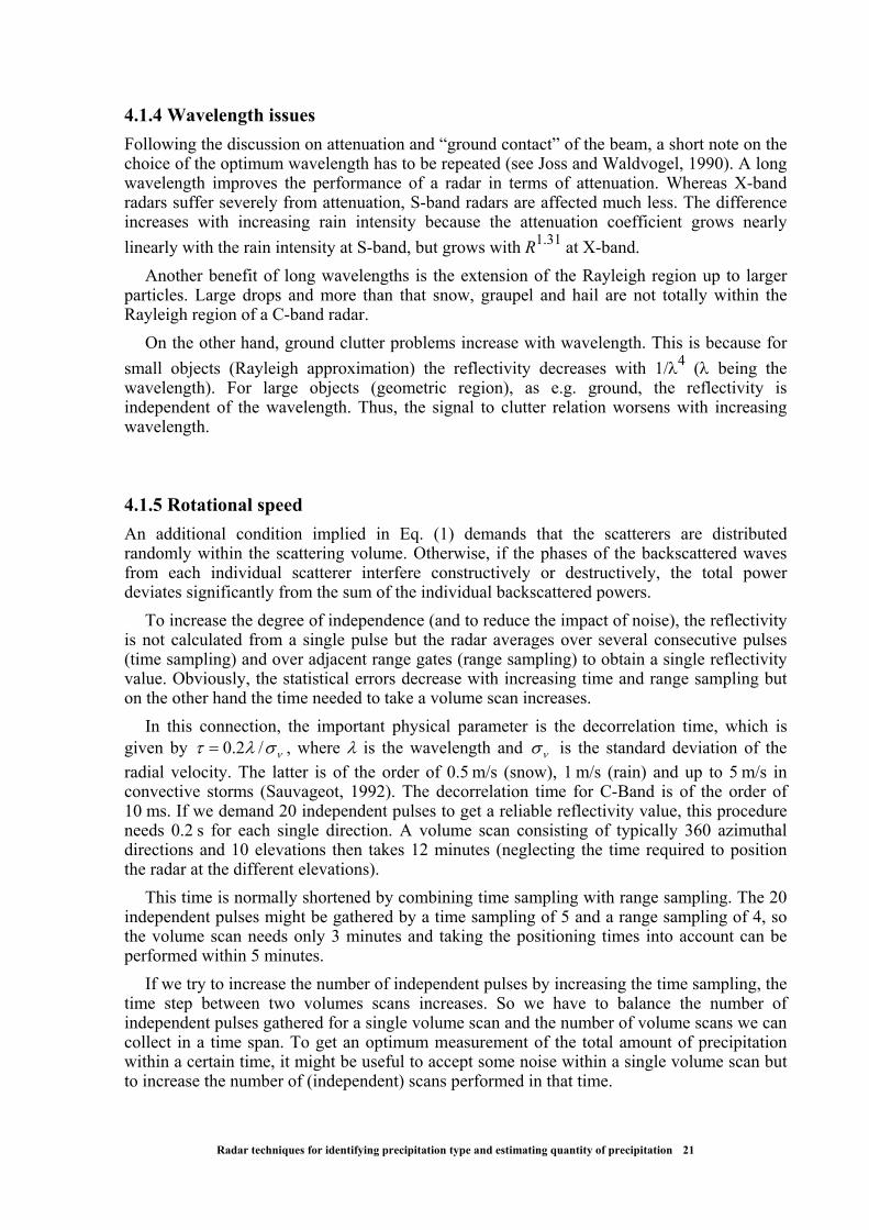
4.1.4 Wavelength issues Following the discussion on attenuation and “ground contact” of the beam, a short note on the choice of the optimum wavelength has to be repeated (see Joss and Waldvogel, 1990). A long wavelength improves the performance of a radar in terms of attenuation. Whereas X-band radars suffer severely from attenuation, S-band radars are affected much less. The difference increases with increasing rain intensity because the attenuation coefficient grows nearly linearly with the rain intensity at S-band, but grows with R1.31 at X-band.

Another benefit of long wavelengths is the extension of the Rayleigh region up to larger particles. Large drops and more than that snow, graupel and hail are not totally within the Rayleigh region of a C-band radar.

On the other hand, ground clutter problems increase with wavelength. This is because for small objects (Rayleigh approximation) the reflectivity decreases with 1/λ4 (λ being the wavelength). For large objects (geometric region), as e.g. ground, the reflectivity is independent of the wavelength. Thus, the signal to clutter relation worsens with increasing wavelength.

4.1.5 Rotational speed An additional condition implied in Eq. (1) demands that the scatterers are distributed randomly within the scattering volume. Otherwise, if the phases of the backscattered waves from each individual scatterer interfere constructively or destructively, the total power deviates significantly from the sum of the individual backscattered powers.

To increase the degree of independence (and to reduce the impact of noise), the reflectivity is not calculated from a single pulse but the radar averages over several consecutive pulses (time sampling) and over adjacent range gates (range sampling) to obtain a single reflectivity value. Obviously, the statistical errors decrease with increasing time and range sampling but on the other hand the time needed to take a volume scan increases.

In this connection, the important physical parameter is the decorrelation time, which is given by νσλτ /2.0= , where λ is the wavelength and νσ is the standard deviation of the radial velocity. The latter is of the order of 0.5 m/s (snow), 1 m/s (rain) and up to 5 m/s in convective storms (Sauvageot, 1992). The decorrelation time for C-Band is of the order of 10 ms. If we demand 20 independent pulses to get a reliable reflectivity value, this procedure needs 0.2 s for each single direction. A volume scan consisting of typically 360 azimuthal directions and 10 elevations then takes 12 minutes (neglecting the time required to position the radar at the different elevations).

This time is normally shortened by combining time sampling with range sampling. The 20 independent pulses might be gathered by a time sampling of 5 and a range sampling of 4, so the volume scan needs only 3 minutes and taking the positioning times into account can be performed within 5 minutes.

If we try to increase the number of independent pulses by increasing the time sampling, the time step between two volumes scans increases. So we have to balance the number of independent pulses gathered for a single volume scan and the number of volume scans we can collect in a time span. To get an optimum measurement of the total amount of precipitation within a certain time, it might be useful to accept some noise within a single volume scan but to increase the number of (independent) scans performed in that time.


For shortening of the scanning process, it is possible to use an ‘interlaced’ volume scan: Only some elevations (e.g. the lowest two elevations and then the every second elevation) are used for a short time period (say, 5 minutes) and the rest (plus the lowest two elevations, again) are taken in the following 5-minute time period. Then, in the 10 minutes we have full volume scan and reduced volume reflectivity fields (and reflectivities from the lowest elevations which are suitable for QPE) are available every five minutes.

4.1.6 Spatial resolution The physical quantity that should be averaged is the rain intensity but the primarily measured quantity is the reflectivity, which is nonlinearly related to the rain intensity. Thus averaging in reflectivity introduces a bias. This bias increases with the inhomogeneity of the reflectivity field and with the size of a recorded range gate, i.e. it increases especially with distance from the radar. The largest values are reached when the bright band is partially included in the scattering volume and in convective storms, when horizontal gradients are strong.

Zawadzki et al. (1999) used highly resolved data from a vertically pointing X-band radar to calculate the reflectivity values a radar with a resolution of 1 degree would measure from a distance of 60 km. The standard deviation was between 1.43 dB and 4.34 dB, indicating that the coarse spatial resolution of a radar is in certain situations a significant source of uncertainties.

4.1.7 Additional issues Other errors that can be present in the radar precipitation estimation include reflections received from various non-meteorological targets that include insects, birds, aircrafts, chaffs, solar radiation etc. These errors are usually not too serious but there are some considerable exceptions. Specific problems, especially for nowcasting, can be caused by ships that are difficult to distinguish from meteorological targets automatically (Koistinen et al., 2003).

There can be problems related to the time discretization of the radar measurement. If the precipitation systems move or develop sufficiently fast, then the integration from the discrete rain rate estimations results in a precipitation field that is artificially discontinuous. Hannesen and Gysi (2002) proposed a correction method which is based on derived motion vectors and the integration along the path which passes the areal element (pixel) between two successive radar images. This problem has also been discussed by Fabry et al. (1994) and by Blanchet et al. (1991).

4.2 Errors of radar-based QPE due to changing meteorological conditions Removing all the non-meteorological targets, however difficult, is only a first step towards reasonable radar-based QPE. Even if it were successfully completed, it could not be guaranteed that the precipitation estimate is accurate or stable. This is because of the large variety of meteorological conditions and processes influencing the precipitation; they are sometimes beneficial and improve the precipitation estimate but in other cases they can have adverse effects in terms of reliable radar detection. For successful utilization of radar estimates, good knowledge of these errors and theirs characteristics according to the particular meteorological situation is crucial.

Some of the “meteorological” errors are schematically depicted at Figure 5; note that the meteorological errors are also influenced by the beam propagation.


Figure 5. Diagram of typical meteorological errors of radar-based QPE of stratiform (top) and convective (bottom) precipitation. The influence of vertical profile of reflectivity and type of precipitation (along with range-dependent width and height of the radar beam) dominates in stratiform region while the QPE in convective processes is often influenced by the presence of the updrafts, downdrafts and hail. Precipitation-induced attenuation depends on the position of the particular storm cells and the radar site(s) and is significant especially in heavy rainfalls. High wind increases the possibility of pronounced seeder-feeder orographic enhancement, typical rather for stratiform precipitation.

Remark: The horizontal extent of the storm cells (bottom) is artificially amplified for better depiction.


4.2.1 Z-R relationship, particle size distribution

The Z-R relation ( ) is surely the best-known error source for most users. Each hydrometeor contributes to the radar reflectivity proportional to the 6

baRZ =th power of its diameter d

whereas it contributes to rain intensity roughly with the 3.7th power of d, see Eqs. (2), (4) and (5). Thus, as long as one only measures the integral reflectivity, one needs assumptions on the drop size distributions.

Nowadays, it is common practice to apply a single or time-conservative, seasonally-dependent Z-R relationship. The values of a and b are usually 200 and 1.6, respectively, which was proposed by Marshall and Palmer. E.g. the German weather service uses Z=256R1.42. Battan (1973) lists several dozens of Z-R relations in which the precipitation intensity R differs for the same reflectivity Z typically by tens of percents, in some cases by hundreds of percents (Doviak and Zrnic, 1993, see also section 3).

Keeping in mind that Z is calculated by solving Eq. 1 for the reflectivity, tuning of the parameter a is identical to a recalibration of the radar constant. Doelling et al. (1996) argue that parameter b only varies between 1.4 and 1.6 in nearly all cases; therefore it is recommended to leave the b parameter within these values. On the other hand, the value of the b parameter is closely linked to the type of precipitation (see Fig. 2, section 3). For instance, in equilibrium (tropical) rainfall, where there is a balance between coalescence and collisional and spontaneous breakup of drops such that the raindrop size distribution reaches a stationary state, the Z-R relation may even become linear (see Uijlenhoet et al., 2003a).

There are approaches that use tuned Z-R relations that reflect different meteorological situations, e.g. of stratiform and convective precipitation (see Table 1, section 3). To apply those corrections, the different types of precipitation have to be identified e.g. on the basis of absolute reflectivity values, presence of a bright band, strong horizontal gradients of precipitation and vertical extent of the radar echo.

A recent approach is called ‘climatologically tuned Z-R relations’. The method consists in deriving the Z-R relations with respect to long time series of rain gauge data and allows a correction of the range effect, also reflecting the precipitation regime from the climatological point of view.

Using short-term measurements to fit the Z-R relation very often degrades the quality because they lack sufficient representativeness. Deviations due to inhomogeneities in the precipitation are not averaged out over the short durations and unrepresentative gauge or disdrometer measurements are generalized over larger areas. This makes online calibrations tricky and sometimes unreliable.

Collecting more information about the precipitation, e.g. by polarimetric measurements (see section 6) is another way to obtain estimates of the drop size distribution and thus on the Z-R relation.

Finally, the probability matching method (PMM, Rosenfeld et al., 1993) or window probability matching method (WPMM, Rosenfeld et al., 1995) should be mentioned. These procedures assign reflectivities and rain intensity with the same probability density to each other. When fitting the parameters a and b of a standard Z-R relation, medium rain intensities contribute the most to the signal. Thus, outliers of very strong precipitation or very weak precipitation are not managed reliably. Because the PMM allows a much more complicated relation between Z and R, these outliers are better represented.

Studies to find the most suitable Z-R relationship for each precipitation type were motivated by the idea that most of the errors of the precipitation estimate are due to improper


Z-R relationships. As it turned out in last two decades of the 20th century, this was a rather misleading paradigm (see e.g. Joss and Waldvogel, 1990). As Zawadzki (1984) showed, the Z-R related error is a relatively minor factor affecting the accuracy of radar estimates of rain rate. On the average the vertical profile, i.e. the extrapolation from the lowest elevation seen by the radar to the ground, and the problem of visibility are probably the most important effects diminishing the quality of radar measurements.

Current work on improving precipitation measurement from single polarization radar is now oriented towards corrections using vertical profile(s) of reflectivity (Germann and Joss, 2003, Koistinen et al., 2003), see also following section 4.2.2.

4.2.2 Variability of the vertical profile of reflectivity, profile correction The formation and modification of atmospheric precipitation particles during their lifecycle is a complex process that depends on the physical and chemical properties of the atmosphere and on the precipitation particles themselves, especially their phase and size. The change of the physical properties of precipitation considerably affects the measured reflectivity and derived precipitation rate. The significance of the vertical profile, especially in widespread precipitation and at larger distances, was realized only roughly a decade ago (e.g. Joss and Waldvogel, 1990).

What we want to feed into the Z-R relation is the reflectivity value at surface height (0 m above the ground). But what we measure is an average of reflectivity values within the (lowest usable) beam at a certain height given by the height of the beam axis above ground. This averaging in the inappropriate quantity (reflectivity instead of rain intensity) produces an additional bias depending on the variability within each range bin (see also section 4.1.6).

The average vertical profile of reflectivity (VPR) exhibits a general decrease with increasing height, typically by 10 to 20 dBZ to mid-troposphere (Gekat et al., 2003, see also Fig. 6). A well-known feature of the vertical profile of reflectivity is the maximum found in the melting layer (where falling ice particles melt to rain) of typical thickness of a few hundreds meters, called bright band. The enhanced reflectivity in the melting layer can cause an overestimation by a factor of five if used as an estimate of the precipitation on the ground (Joss and Waldvogel, 1990). The influence of the melting layer is especially pronounced in the vicinity of the radar (up to several tens of km) where the bright band has a vertical depth similar to the beam width. At a larger distance from the radar, the influence of the bright band decreases as it can fill only part of the beam that is broadening with the distance. As the radar beam gets more into the snow region above the melting layer at larger ranges, the bright band can partly compensate for the general range-dependent underestimation of precipitation rate (when the bright band is approximately 1 km above the antenna, see Koistinen et al., 2003). At further ranges, the bright band is in nearly all cases below the lowermost height seen by radar (see also Figure 5).


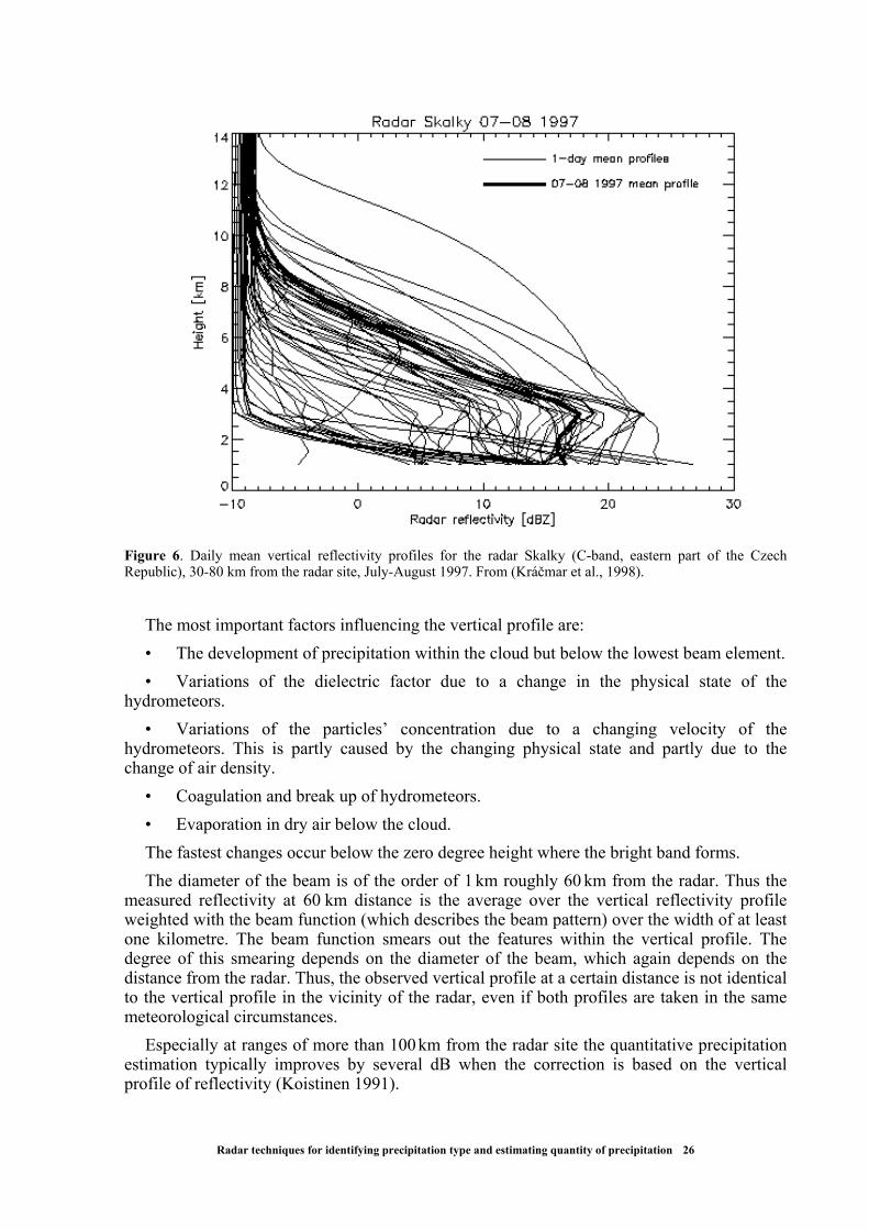
Figure 6. Daily mean vertical reflectivity profiles for the radar Skalky (C-band, eastern part of the Czech Republic), 30-80 km from the radar site, July-August 1997. From (Kráčmar et al., 1998).

The most important factors influencing the vertical profile are: • The development of precipitation within the cloud but below the lowest beam element. • Variations of the dielectric factor due to a change in the physical state of the

hydrometeors. • Variations of the particles’ concentration due to a changing velocity of the

hydrometeors. This is partly caused by the changing physical state and partly due to the change of air density.

• Coagulation and break up of hydrometeors. • Evaporation in dry air below the cloud. The fastest changes occur below the zero degree height where the bright band forms. The diameter of the beam is of the order of 1 km roughly 60 km from the radar. Thus the

measured reflectivity at 60 km distance is the average over the vertical reflectivity profile weighted with the beam function (which describes the beam pattern) over the width of at least one kilometre. The beam function smears out the features within the vertical profile. The degree of this smearing depends on the diameter of the beam, which again depends on the distance from the radar. Thus, the observed vertical profile at a certain distance is not identical to the vertical profile in the vicinity of the radar, even if both profiles are taken in the same meteorological circumstances.

Especially at ranges of more than 100 km from the radar site the quantitative precipitation estimation typically improves by several dB when the correction is based on the vertical profile of reflectivity (Koistinen 1991).


Large errors - requiring large corrections in radar estimates of surface precipitation - are likely to occur in the following meteorological situations:

1. If precipitating clouds are shallow, i.e. in cold climates or temperate climates during the winter, the radar beam is only partially filled with precipitation at ranges far from the radar (Kitchen and Jackson 1993). Additional underestimation occurs if ice particles fill the measurement volume aloft while the dielectric factor, which is actually used in the radar equation, is that of water (see section 4.2.4). It is not uncommon for the error in surface estimates of rainfall or in radar reflectivity factor to exceed 5 dB at a range of 100 km and to increase dramatically at farther ranges. The effect of beam overshooting is further pronounced if part of the radar beam is blocked. In the worst case the precipitation is not seen by the radar at all and no correction is possible (see e.g. Koistinen et al., 2003).

2. If the beam intercepts the bright band this may lead to overestimation of surface rainfall up to 5-10 dB. The overestimation can cover (i) a ring-shaped area at a fixed range from a radar (if the rainfall product is based on a PPI image and the bright band is spatially homogeneous) or (ii) it can behave stepwise as a function of range (if the selected CAPPI level coincides with the height of the melting level and no interpolation has been applied when the CAPPI is calculated from rings of the original PPI measurements). For description of this effect, see e.g. Sanchez-Diezma et al. (2000).

3. Strong evaporation below the observation height leads to overestimation of the precipitation reaching the ground. This is typical in widespread frontal Altostratus clouds preceding warm and occluded fronts or at the trailing edge of cold fronts of ana-type.

4. In hilly or mountainous terrain orographic growth of hydrometeors below the height of a radar measurement may result in considerable (up to 6 dB) underestimation of precipitation at the ground. This orographic enhancement is dealt with in more detail in section 4.2.3.

The main problem in the operational application of a correction scheme is the unknown vertical profile of reflectivity (VPR) or precipitation profile i.e. the ratio of observed beam smoothed values aloft and the ground truth at each location in each moment of measurement. Prior to any vertical reflectivity profile correction one should consider how accurately the time-space structure of the profile should be known in order to improve radar derived precipitation amounts significantly. The experience gained to date suggests that profiles derived from measurements near the radar and integrated over much longer time periods than the actual accumulation period of precipitation will help considerably.

A coarse way to take into account the mean beam overshooting and shielding due to mountains and earth curvature is to determine empirical range dependent adjustment factor based on long-term gauge-radar comparisons at the same locations.

The next step is to use seasonal mean profiles (Joss and Pittini, 1991) or climatological classes based on synoptic weather types (Brown et al., 1991). These profiles can be estimated without actually calculating the mean of all measured profiles during a season. If the large synoptic scale variation of the melting level height is taken into account, the averaging time of reflectivity profiles cannot be longer than approximately one day. It was found that the use of mean daily reflectivity profiles reduced the bias in radar-derived daily rainfall estimates by up to 6 dB (Koistinen, 1991).

Accurate correction of the effect of error in the vertical profile, especially in cases of very short accumulation periods (e.g. 10 minutes) requires knowledge of the time-space distribution of the profile. Much research is being carried out on in various countries (Switzerland, Spain, France, USA, …) to develop acceptable correction algorithms based on the availability of volume scans.

For a thorough discussion of the determination of the VPR with respect to the radar beam


geometry and sampling scheme see e.g. Andrieu and Creutin (1995) who propose a method that is less affected by the radar beam geometry and smoothing. Leaving aside the issues regarding the identification of the profile by the radar, the weakest point of these schemes is still the lack of representativeness of the profile for the areas where the VPR correction is applied. Although the uncertainty about the ‘true’ but unknown profile in the area of interest (where the VPR correction is applied) remains relatively large, the correction is still able to reduce the range dependency of the bias (see e.g. Novák and Kráčmar, 2001). Then it makes the radar estimate more suitable for the mean field adjustment by the rain gauges measurements. Otherwise, if the VPR correction is not applied, then the possible rain gauge adjustment must often utilize a bias that is dependent on the range (see, e.g. Michelson et al., 2000), which can be also considered as a coarse VPR correction (see above).

4.2.3 Errors of radar estimates caused by orographic seeder-feeder precipitation enhancement Complex orography not only reduces radar visibility but, under favourable conditions, induces also significant change of precipitation intensity and duration. The orographic enhancement of precipitation can be divided into three categories (after Grey and Seed, 2000):

a) Orography-induced autoconversion (growth of the droplets through collision and coalescence), which can produce only light rain.

b) Seeder-feeder mechanism; the low level cloud is maintained by upslope winds and provide the moisture source that is collected by the drops falling from aloft from ‘seeder’ clouds.

c) Triggered convection that is caused by the wind flow over the hills which triggers potential instability; the convection can be also activated by heating of the slopes in relatively cold air.

The autoconversion is usually not too important from the hydrological point of view and triggered convection can be well captured by radar due its vertical extent. The seeder-feeder enhancement often causes significant error in the radar estimates because it takes place mainly within a few hundred meters above the ground. Even 50 m high hills can produce an enhancement of 10-40% in the lowest 500 m (Grey and Seed, 2000). The seeder-feeder mechanism causes two types of problems for radar estimates: (i) the radar detection often suffers from reduced visibility in mountainous areas and (ii) at the same time significant enhancement can occur very close to the ground, at the heights that are barely seen by the radar. The lowest usable beam is then often able to capture only the seeder clouds and at most only a part of the feeder area, which results in very significant underestimation (Collier, 1996, Gray and Seed, 2000). Moreover, the orographic precipitation usually shows specific type of the drop size distribution, which further worsens the radar underestimation (Rosenfeld and Ulbrich, 2002, see also section 3).

Collier (1996) advises that the radar should be sited so that it can observe the low level precipitation directly, but this is not always possible. For more successful assessment and anticipation of this error additional information sources are needed, e.g. direct observation and NWP models. Even a climatologically derived relationship between humidity and wind at 800 m above sea level and the magnitude of the seeder-feeder enhancement can partly help (Kitchen et al., 1994, Harrison et al., 2000). However, the orographic enhancement effect is not simple, as Grey and Seed note, and they also add: ‘If radar were to be used to increase the lead-time for flood forecasting, then it would necessary to forecast, in advance, the manner in which the enhancement will be manifestated.’


4.2.4 Dielectric Factor

Knowledge of the dielectric factor 2K provides information about the physical state of the

hydrometeors. The value of 2K for water is approximately 0.93 (depending weakly on temperature and wavelength), for ice it is roughly 0.18, i.e. 5 times smaller. The radar software always assumes as a default setting that precipitation consists of liquid drops, thus it calculates with a fixed dielectric factor of 0.93. This leads to an underestimation of the reflectivity within convection (see Eq. 1). Nevertheless, this is only one of several problems due to graupel and hail (see also sections 4.2.8, 4.2.9 and 5.2).

In stratiform precipitation there is a clear separation of ice and water: Above the bright band ice particles dominate, below you find water phase and the bright band contains a mixture of both constituents. In these cases the dielectric factor contributes to the vertical profile and the VPR correction (see above) deals with it inherently.

In convective cells the different states are mixed and the separation is not possible. Dual polarization radars might provide an estimate of the mixing ratio of the liquid and frozen components (see section 6) but without a dual polarization facility this ratio is not available.

There are techniques to identify areas with convection within radar images. High reflectivity values, large horizontal gradients, vertical profile and large vertically integrated liquid water contents are used to separate these areas from the rest. Nevertheless, even if one can identify a thunderstorm, no information about the relative proportions of ice and water is available from a single polarization radar.

4.2.5 Errors caused by attenuation in precipitation Radar radiation is attenuated by atmospheric gases and hydrometeors. Attenuation is strongly dependent on the wavelength; S-band radar (approx. 10 cm wavelength) is much less affected by attenuation then X-band (approx. 3 cm wavelength).

Among the gases in the atmosphere, oxygen and water vapour cause the most attenuation. In most cases, the attenuation due to oxygen (which is of the order of 7×10-3 dB/km) is more intense then that caused by water vapour. This static part of attenuation is normally corrected for by the radar signal processor, which uses a user-defined value for the attenuation coefficient to correct the data.

The more intense and more problematic part of the attenuation is due to the precipitation itself. It is possible to estimate the attenuation by power laws of the form

K=aRb, (25)

where K is the attenuation coefficient in dB/km and R the rain rate in mm/h. In case of rain these laws read (see Sauvageot, 1992) as K=0.3×10-3R1.00 at S-band, K=2.2×10-3R1.17 at C-band, and K=7.4×10-3R1.31 at X-band for one-way attenuation. At a range of 100 km and a (constant) rain rate of 1 mm/h a two-way attenuation of 0.06 dB, 0.44 dB and 1.48 dB is observed for S, C and X bands, respectively. A cell with a diameter of 5 km and a rain intensity of 40 mm/h produces a two-way attenuation of 0.12 dB, 1.6 dB and 9.3 dB, respectively. In snow the attenuation is weaker and in the bright band it can be even more intense. For further reading, see Delrieu et al. (1991).

Due to this sensitivity and the effect that an overestimation of the attenuation in a nearer range gate produces an even worse overestimation in a further range gate, the gate-to-gate correction schemes prove to be unstable in many cases (e.g. Hildebrand, 1977, Hitschfeld and


Bordan, 1953, Bringi and Chandrasekhar, 2001). The chance for instabilities increases with the attenuation that has to be removed from the data: The more we need attenuation correction the worse it works. This is the reason why attenuation correction is not operational at any weather service. Although occasional attempts of a correction scheme are still reported (see e.g. a proposal to use a variational method by Berenguer et al., 2002), the most promising algorithms are based on the use of the differential phase shift for dual-polarization radars.

4.2.6 Additional attenuation by water on the radome Water on the radome causes an additional attenuation and a broadening of the beam width. These effects are well known not only in the radar community but also e.g. in the (satellite) communication field (Anderson, 1975). As long as the water stays in the form of droplets on the radome, the effect is not very strong. Separate droplets behave as additional rain. But as soon as the water forms rivulets or even a closed film on the radome, the attenuation increases significantly.

Therefore, radomes are manufactured with a repellent coating, which should inhibit the formation of water films. This coating degrades due to dirt and dust and physical and chemical interaction with the environment. The water film thickness at a certain point on the radome depends on the rain intensity, wind speed and direction, state of the radome surface and the position of that point (especially the slope).

The variation of the film thickness causes an additional beam distortion that can be disturbing, especially if it leads to additional ground clutter in the echoes.

This effect is difficult to be removed, mainly because exact information on the water film thickness is not available. Experiments with artificial precipitation from a fire brigade on a radome produced an attenuation of roughly 5 dB (one direction) due to an estimated equivalent rain rate of about 100 mm/h on a 5-year-old radome (Manz et al., 1999). This attenuation corresponds to an error of a factor 4.5 in the rain rate.

This additional attenuation can obviously be very important. It varies with azimuth and elevation of the antenna and it changes in time as rapidly as the rain rate varies at the radar location. Nevertheless, there is no operational service applying any correction routine to deal with this error. It is not easy to remove this error afterwards, because it varies with time and with the direction from the radar. Thus it is a rather inhomogeneous distortion on short time scales.

4.2.7 Shape of the rainfall droplets The derivation of Eq. 1 uses the assumption, that the scatterers are spherical. This is realistic for small drops but the drops of the order of 1 mm or larger get oblate. Frozen hydrometeors, especially snow, grow in a nearly arbitrary shape and the error is larger. In snow this error is one of several additional errors in determining the (equivalent) rain rate. No investigation that separates this error from the other problems in snow is known to the authors.

The deviation of the large drops from the spherical shape is used in dual polarization radars to estimate information about the drop size distribution through the difference of reflectivity of horizontal vs. vertical polarisation. This difference is measured as the differential reflectivity ZDR:

⎟⎟⎠

⎞⎜⎜⎝

⎛=

V

HDR Z

ZZ log10 , (26)


where ZH and ZV denote the reflectivity of a horizontally or vertically polarized signal, respectively. ZDR reaches values of up to 5 dB in rain. The details will be discussed in the section 6.

4.2.8 Precipitation Particles of size beyond Rayleigh approximation To allow the reflectivity of a single scatterer to be calculated by the Rayleigh approximation, as it is done in radar meteorology, the scatterer has to be small compared to the wavelength. Small means that the diameter should be 10 to 16 times smaller than the wavelength. This means that the largest particle should be smaller than 10 mm, 5 mm and 3 mm for S-, C- and X-band, respectively. In moderate climates raindrops are normally smaller than 5 mm. In tropical rain, drops of 8 mm are often observed. Frozen hydrometeors may be even larger than 10 mm. These large particles do reflect much less than assumed by the Rayleigh approximation. Thus, they are estimated to be smaller than they are in reality. On the other hand, these large particles are not properly described by the usual drop size distributions that underlie the Z-R relation.

Finally, hailstones produce much less precipitation than rain of the same reflectivity. An example: A hailstone of 10 mm produces (in Rayleigh approximation) a reflectivity of 106

mm6. Due to the fact, that it is not in the Rayleigh region we assume it to reflect only half this value: 5× 105

mm6. Its volume is 535 mm3. To produce the same reflectivity we need 32 drops with a diameter of 5 mm. Their total

volume is nearly 2100 mm3, roughly 4 times the volume of the hailstone. Thus, they contribute much more rain than the hailstone, notwithstanding their smaller fall velocity.

Large hailstones violate the Rayleigh approximation as well as the Marshall-Palmer drop size distribution. Finally, they lead to a severe overestimation of rain intensity. There are heuristic methods to reduce this overestimation. Among the simplest ones you can find using the ‘hail cap’, i.e. truncation of the maximum used reflectivity/rainrate to predefined value (e.g. Fulton et al., 1998, see also Table 2). Another approach assumes that rain intensities of more than 200 mm/h should be corrected by unkorrkorr RhmmR 200]/[ = .

In fact, these very intense events last in most cases only for short durations so the integrated amount of rain is normally not large. On the other hand this infrequency makes it difficult to find more sophisticated correction themes than the one cited above.

4.2.9 Errors caused by different precipitation type As noted in previous sections, the Z-R relationship and the radar equation assume liquid water and a spherical shape of the droplets of size not exceeding some limits. However, these assumptions are often far from the reality; especially in cold climate (or cold season in temperate climate) the radar frequently measures snowfall and instead of using the Z-R relationship for rainfall, Ze-S (equivalent reflectivity – snowfall [mm/h]) relationship with different coefficients should be applied. For detailed studies and independent sampling of precipitation rate one must not forget the problem of a different factor 2K for water and ice (see section 4.2.4) that is usually kept constant all year round.

However, the error caused by unsuitable use of Z-R/Ze-S relationship is usually less important than more serious problems connected with snowfall. The general decrease in vertical depth of snowfall-producing clouds in a cold climate (or season) results in more


severe underestimation at long ranges. More information about these effects and possible corrections can be found in Koistinen et al. (2003).

One of the difficulties that are usually encountered in warm seasons is the presence of hail as mentioned in the previous chapter (see also chapter 4.2).

4.2.10 Updrafts and downdrafts According to Gunn and Kinzer (1949, in Doviak and Zrnic, 1993), the typical vertical velocities of raindrops in stagnant air are between 2 and 8 m/s; the raindrops of the 0.6 mm and 4 mm diameter fall at the speed 2 m/s and 8 m/s, respectively (at the air pressure of 1013 hPa and air temperature of 20ºC). In the middle of the troposphere the raindrop velocities are about 30-40% higher due to less air density.

The Z-R relation requires assumption that the raindrops are falling in a still air. The situation changes in convective storms where updrafts and downdrafts up to tens of m/s occur (see also Fig. 5). In an updraft the radar must overestimate surface precipitation rate because the air current suspends the precipitation particles in the air. In the downdraft the situation is more complex. It is obvious that at the height typical for radar measurement of precipitation, roughly about 1 km above the surface or more, the rainfall rate relative to the earth surface is greater than the radar estimate that assumes still air because of the vertical velocity of the falling air. However, the vertical velocity of the air at the horizontal earth surface is zero. It means that the downdrafts diverges at the surface and thus increases the area that is hit by the precipitation present in the downdraft (Kessler, 1987, Lee, 1988 in Doviak and Zrnic, 1993). Then the downdraft presence mainly results in underestimating the area hit by the heavy precipitation. Only if hail is present, the underestimation caused by downdraft may not be so pronounced (Collier, 1996).

The errors caused by downdrafts and updrafts, which can be up to several dB (Collier, 1996, Joss and Waldvogel, 1990), can be reduced by integrating the rainfall over a sufficiently large area where these effects are likely to compensate. Thus, the recommended reasonable area for mean areal estimates should be equal or more than the typical area of convective storm cells, which is typically about ten square kilometres. If smaller areas are used when analysing convective precipitation, these effects are likely to be more significant.

4.2.11 Additional problems In addition to the previous list of errors, we have to mention drift by the upper wind, three-body scattering signature caused by additional scattering between hail and ground and second trip echo caused by intensively backscattering targets beyond the maximum unambiguous range (see e.g. Doviak and Zrnic, 1993). However, these types of error are generally smaller than the ones described above.

4.2.12 Summary of the meteorological errors The meteorological errors are summarized in Table 2 which is adapted from Austin, 1987 (in Collier, 1996). It gives the overview of the expected magnitudes of the errors and the proposed action that may be taken or the compensating effects which can occur.


Table 2. The effects of meteorological factors on values of equivalent rainfall rate deduced from radar measurements and conditions under which they are significant (adapted from Collier, 1996).

Factor

Magnitude of the effect and situations where it is significant

Methods for compensations

Drops larger than average in intense convective storms; reflectivity increased by 1-2 dB

Use of relation Z=400R1.3 or similar *;raingauge adjustment

Drops smaller than average in warm-frontal rain; reflectivity decreased by 3-4 dB

Use of relation Z=100R1.4 or similar *;raingauge adjustment

Variations in the raindrop-size distributions

Any other deviation from average drop-size distribution is usually too small to be detected or is masked by other effects

Predominant factor in intense convective storms (Max Z ≥ 53 dBZ); may increase reflectivity in storm cores by 10 dB or more above that of the rain alone

Limiting R (or Z) to a maximum value (“hail cap”); usually Rmax ≈100 mm/h (from 75 to 150 mm according to the climate type – Fulton et al., 1998); some compensation by downdraft effect **

Enhancement of signal by presence of hail

Probably 4-5 dB enhancement in moderate convective storms (45 dBZ ≤ max Z ≤ 53 dBZ) which are non-frontal

Automatically compensated for by downdraft effect **

Predominant factor in moderately convective storms which are associated with cold fronts or stationary fronts. Reflectivity in storm cores diminishes by 4-5 dB

Use of relation Z=230R1.2 *;

Some compensation by updraft (overestimating) effect **

Diminution of reflectivity by downdrafts associated with heavy rain in convective cells

Similar effect in intense convective storms and in non-frontal moderate convective storms

Automatically compensated for by hail effect or updraft effect **

Signal enhancement by melting snow

Significant factor in all stratiform rain. When ‘bright band’ is in the radar beam, reflectivity may be 1-5 dB stronger than that of the rain alone

Limiting measurement to region below the melting layer; correction procedures using estimates of reflectivity profile

Low-level growth of raindrops in fog or stratus clouds

Occurs when fog or low stratus is present. Increase in rainfall rate unlikely to be more than 25 % in light rain or 15 % in heavy rain (except orographic enhancement – see below)

Recognition of possible underestimation by radar when fog is present; raingauge adjustment; correction procedures using knowledge of reflectivity profile


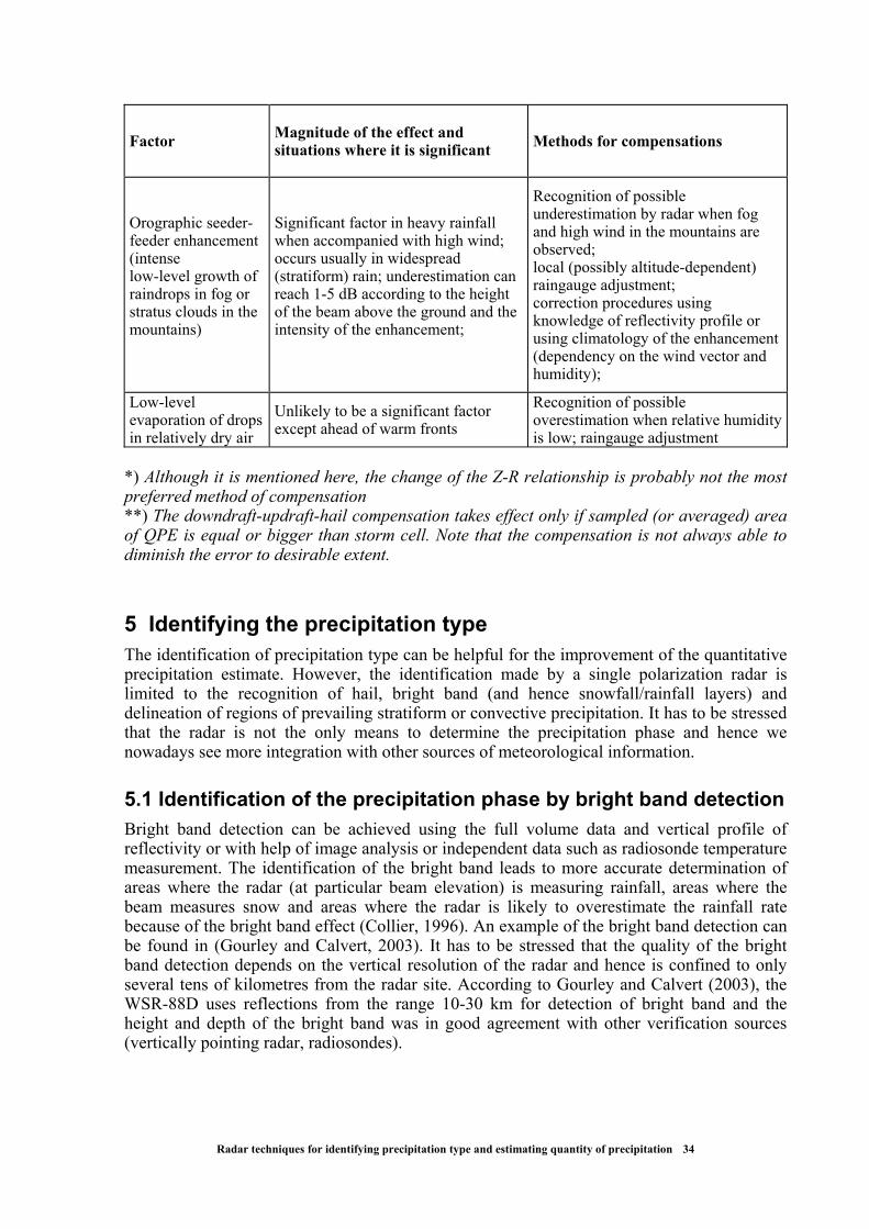
Factor

Magnitude of the effect and situations where it is significant

Methods for compensations

Orographic seeder-feeder enhancement (intense low-level growth of raindrops in fog or stratus clouds in the mountains)

Significant factor in heavy rainfall when accompanied with high wind; occurs usually in widespread (stratiform) rain; underestimation can reach 1-5 dB according to the height of the beam above the ground and the intensity of the enhancement;

Recognition of possible underestimation by radar when fog and high wind in the mountains are observed; local (possibly altitude-dependent) raingauge adjustment; correction procedures using knowledge of reflectivity profile or using climatology of the enhancement (dependency on the wind vector and humidity);

Low-level evaporation of drops in relatively dry air

Unlikely to be a significant factor except ahead of warm fronts

Recognition of possible overestimation when relative humidity is low; raingauge adjustment

*) Although it is mentioned here, the change of the Z-R relationship is probably not the most preferred method of compensation **) The downdraft-updraft-hail compensation takes effect only if sampled (or averaged) area of QPE is equal or bigger than storm cell. Note that the compensation is not always able to diminish the error to desirable extent.

5 Identifying the precipitation type The identification of precipitation type can be helpful for the improvement of the quantitative precipitation estimate. However, the identification made by a single polarization radar is limited to the recognition of hail, bright band (and hence snowfall/rainfall layers) and delineation of regions of prevailing stratiform or convective precipitation. It has to be stressed that the radar is not the only means to determine the precipitation phase and hence we nowadays see more integration with other sources of meteorological information.

5.1 Identification of the precipitation phase by bright band detection Bright band detection can be achieved using the full volume data and vertical profile of reflectivity or with help of image analysis or independent data such as radiosonde temperature measurement. The identification of the bright band leads to more accurate determination of areas where the radar (at particular beam elevation) is measuring rainfall, areas where the beam measures snow and areas where the radar is likely to overestimate the rainfall rate because of the bright band effect (Collier, 1996). An example of the bright band detection can be found in (Gourley and Calvert, 2003). It has to be stressed that the quality of the bright band detection depends on the vertical resolution of the radar and hence is confined to only several tens of kilometres from the radar site. According to Gourley and Calvert (2003), the WSR-88D uses reflections from the range 10-30 km for detection of bright band and the height and depth of the bright band was in good agreement with other verification sources (vertically pointing radar, radiosondes).


5.2 Identification of hail 5.2.1 Introduction Hail precipitation is associated with very high radar reflectivities. The conversion to precipitation rates using the conventional Z-R relationship will generally give rise to a significant overestimation of the on-ground precipitation accumulation as mentioned in section 4.2.8. Besides, hail precipitation is responsible for relatively high attenuation of the radar beam through absorption and scattering. As a result, radar estimates of precipitation behind these hail cells can be significantly underestimated. For these reasons, a reliable detection of the presence of hail is of great importance for hydrological applications.

5.2.2 Hail development processes The microphysical processes responsible for hail development are not yet completely understood. Ice particles may form in a cloud if the temperature drops below zero. However, the transformation to ice does not take place readily and the ice phase is frequently observed only as cloud temperatures approach –20°C (Pruppacher and Klett, 1997). Liquid water that is colder than 0°C is called supercooled. At temperatures below 0 °C, the coexistence of supercooled water drops and ice particles is an important factor for the development of hailstones. Three different mechanisms are responsible for the growth of ice particles.

The first mechanism is the collision and aggregation of ice particles. This mechanism is often referred to as clumping and is mainly active at the initial stage of the particle growth. The second mechanism is deposition, i.e. water vapour diffusion to the ice particles. The presence of liquid water ensures the diffusional growth of ice crystals at the expense of water drops through the Bergeron process (Bergeron, 1933). This process relies primarily on the fact that the saturation vapour pressure with respect to ice is less than the saturation vapour pressure with respect to water. The last mechanism is riming, i.e. the collection and freezing of water drops colliding with ice particles. The initial growth of ice crystals is primarily through clumping and vapour deposition until they are large enough to begin riming (Jameson and Johnson, 1990). When riming of an ice particle has proceeded to the stage where the features of the original ice crystal are no longer visible, the ice particle is referred to as a graupel. Rimed particles that have reached a diameter larger than 5 mm are called hailstones.

The production of large hailstones needs a rapid growth of ice particles through the above-mentioned mechanisms. Favourable conditions are found in intense thunderstorms where water and ice coexist in the central updraft. There is a positive relationship between the apparent strength of a storm (strength and size of updraft) and the size of hail that it produces (Ray, 1990). Growth of hailstones is highly influenced by the flow dynamics within the thunderstorm (Heymsfield et al., 1980; Nelson, 1983). The interactions between microphysical processes and thunderstorm flow fields are complex. The trajectories of hailstones depend on the type of storm. In supercell storms, it is thought that most hail mass is acquired during a single pass across the updraft (e.g. Browning and Foote, 1976). More complex trajectories can be found in multicells where hailstones may recirculate in different cells of the thunderstorm complex, resulting in successive growth cycles. Nelson (1983) concludes that the most critical storm feature for large hail to be produced is the presence of a broad area of moderate updraft ensuring a sufficient residence time in a favourable growth environment.


5.2.3 Radar-based hail detection methods The most efficient technique for discrimating hail from water is given by dual polarization radars (e.g. Seliga et al., 1982). Reflectivities in the horizontal (ZH) and vertical polarizations (ZV) are similar for spherical hailstones, which is not the case for non-spherical raindrops. The widely used parameter in this technique is the differential reflectivity (see Eq. 26).

Very large reflectivities together with low values of differential reflectivity are the signature of hail precipitation.

Another technique for hail detection is the dual-wavelength algorithm that was first proposed by Atlas and Ludlam (1961). This method is based on the measurements from a dual wavelength radar and makes use of the reflectivity dependence on the wavelength, which is much higher for hailstones than for water drops. This technique does not receive the same degree of attention as the dual polarization but some new developments have been recently published (Feral et al., 2003).

Most radars of currently operational networks are single wavelength and single polarization radars. Various methods have been proposed for detecting hail using reflectivity measurements from this type of radar. In this section, we give a short overview of the currently used methods. An extended review can be found in Holleman (2001).

The most straightforward way for detecting hail is based on the Pseudo Constant Altitude Plan-Position Indicator product (Pseudo CAPPI). This product is generated from a radar scan at multiple elevations. The Pseudo CAPPI represents the reflectivity values at a given altitude above mean sea level. It is produced by interpolating between the reflectivity data from different elevations. At short ranges, where the highest radar beam is lower than the selected altitude, the reflectivity data are taken from the highest elevation. At long ranges, where the lowest beam is above the selected altitude, the data are taken from the lowest elevation. For the radar of Wideumont, the selected altitude is 1500 m and the Pseudo-CAPPI is generated every 5 minutes from a scan at 5 elevations (Fig. 7).

Figure 7. Pseudo-CAPPI 1500 m for the radar of Wideumont (Belgium) derived from 5 scans at different elevation angles (in degrees).

Large hail stones give rise to very high reflectivities that could not be obtained from rain drops. Mason (1971) proposes a reflectivity threshold of 55 dBZ for distinguishing between


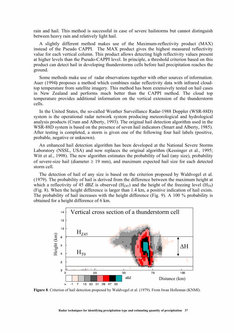
rain and hail. This method is successful in case of severe hailstorms but cannot distinguish between heavy rain and relatively light hail.

A slightly different method makes use of the Maximum-reflectivity product (MAX) instead of the Pseudo CAPPI. The MAX product gives the highest measured reflectivity value for each vertical column. This product allows detecting high reflectivity values present at higher levels than the Pseudo-CAPPI level. In principle, a threshold criterion based on this product can detect hail in developing thunderstorms cells before hail precipitation reaches the ground.

Some methods make use of radar observations together with other sources of information. Auer (1994) proposes a method which combines radar reflectivity data with infrared cloud-top temperature from satellite imagery. This method has been extensively tested on hail cases in New Zealand and performs much better than the CAPPI method. The cloud top temperature provides additional information on the vertical extension of the thunderstorm cells.

In the United States, the so-called Weather Surveillance Radar-1988 Doppler (WSR-88D) system is the operational radar network system producing meteorological and hydrological analysis products (Crum and Alberty, 1993). The original hail detection algorithm used in the WSR-88D system is based on the presence of seven hail indicators (Smart and Alberty, 1985). After testing is completed, a storm is given one of the following four hail labels (positive, probable, negative or unknown).

An enhanced hail detection algorithm has been developed at the National Severe Storms Laboratory (NSSL, USA) and now replaces the original algorithm (Kessinger et al., 1995; Witt et al., 1998). The new algorithm estimates the probability of hail (any size), probability of severe-size hail (diameter ≥ 19 mm), and maximum expected hail size for each detected storm cell.

The detection of hail of any size is based on the criterion proposed by Waldvogel et al. (1979). The probability of hail is derived from the difference between the maximum height at which a reflectivity of 45 dBZ is observed (HZ45) and the height of the freezing level (HT0) (Fig. 8). When the height difference is larger than 1.4 km, a positive indication of hail exists. The probability of hail increases with the height difference (Fig. 9). A 100 % probability is obtained for a height difference of 6 km.

Hei

ght (

km)

Distance (km)

Vertical cross section of a thunderstorm cell

∆H

HZ45

HT0Hei

ght (

km)

Distance (km)

Vertical cross section of a thunderstorm cell

∆H

HZ45

HT0

Figure 8. Criterion of hail detection proposed by Waldvogel et al. (1979). From Iwan Holleman (KNMI).


The new algorithm has been evaluated through comparison with ground-truth data collected during a field experiment in the summer months of 1992 and 1993. Kessinger et al. (1995) note a significant improvement with respect to the initial version. The hail detection method based on Waldvogel has been operationally implemented at KNMI (Royal Netherlands Meteorological Institute) and tested on an extended verification dataset in the summer months of 1999 and 2000 (Holleman, 2001). The results show that this method performs substantially better than any other tested methods. The verification results have been used to adjust the function that relates the probability of hail (POH) to the height difference between the freezing level and the maximum height of the 45 dBZ reflectivity.

The following expression is currently used in the operational hail detection algorithm at KNMI:

045),(133.0319.0 ZTZ HHHkmHPOH −=∆∆+= (27)

As can be seen on Figure 9, the linear expression obtained by Holleman (2001) differs significantly from the original relation used by Witt et al. (1998). This is probably due to differences in climatological conditions associated with hail.

-1-2 -1-2

Figure 9. Probability of hail as a function of the difference between the maximum height at which a reflectivity of 45 dBZ is observed (HZ45) and the height of the freezing level (HT0). The black stepwise line gives the relation used by Witt et al. (1998) and the blue line the expression obtained by Holleman (2001). Figure adapted from Witt et al. (1998).

In particular, the climatology of the height of the freezing level may significantly influence

the POH relation. The method of Waldvogel using the formulation (1) has been implemented at the Royal Meteorological Institute of Belgium and tested on reported hail events in the summer 2002 (Delobbe et al., 2003). For 22 cases out of 23, a probability of hail at least equal to 50 % was found at less than 10 km from locations where hail fall was reported.

As mentioned above, the NSSL has also developed algorithms for the detection of severe hail (diameter ≥ 19 mm), and the prediction of maximum expected hail size (Witt et al., 1998). The severe hail algorithm is based on a severe hail index (SHI) derived from the


vertical profiles of reflectivity and temperature. The vertical profile of reflectivity is first converted into a vertical profile of hail kinetic energy flux and then vertically integrated using a temperature-based weighting function. The maximum expected hail size is also derived from the SHI using a simple empirical relationship. It must be noted that the verification of severe hail detection algorithms and even more of maximum size predictions is extremely difficult given the highly sporadic nature of severe hail reports.

Vertically integrated liquid water (VIL) is another indicator of the severity of a storm cell which was introduced by Greene and Clark (1972). Reflectivity values can be converted to liquid water contents using a semi-empirical relationship similar to the Z-R relationship used for the conversion of reflectivities to precipitation rates. The vertical integration of the liquid water content is the VIL. However, discriminating between thunderstorms with and without hail using VIL only is not straightforward since there is a large variability in the VIL threshold associated with the presence of hail. A normalized VIL has been proposed by Amburn and Wolf (1997) : the VIL is divided by the height of the top of the thunderstorm cell. This top can be for example determined as the maximum height with a 7 dBZ reflectivity value. The threshold for the normalized VIL is supposed to be more universal than the VIL threshold. Nevertheless there is still no agreement on the most appropriate threshold for operational hail detection method using a normalized VIL indicator.

5.3 Determination of stratiform/convective type of precipitation Stratiform (large-scale, synoptic-scale) precipitation is caused by upward vertical motion over large areas (thousands of sq. kilometres and more) of typical velocities of cm/s as the result of synoptic-scale forcing. From the radar point of view, it usually exhibits well-defined bright band (if the surface precipitation is liquid) and rather low horizontal gradients of precipitation (with some notable exceptions, among others due to orographic enhancement). Detection of such precipitation by radar often encounters significant systematic errors due to bright band effects, attenuation over the large areas of continuous precipitation and rather low vertical depth of the precipitation region, i.e. steep vertical gradient of reflectivity, which results in a pronounced range dependent bias (significant systematic underestimation at far ranges). Under favourable conditions, seeder-feeder orographic enhancement can occur.

Convective precipitation, on the other hand, is caused by nearly vertical air motions of typical velocities of 1 m/s to tens of m/s caused by the atmosphere instability. Convective precipitation shows very high horizontal gradients and large vertical depth. These characteristics mean that the weather radar is the best tool for detecting convective precipitation, but the presence of different types of hydrometeors, especially hail, and storm dynamics (magnitude of updrafts and downdrafts) resulting in fast varying VPR usually result in considerable random error in quantitative precipitation estimates. Large differences can be found especially when comparing rain gauge and radar estimates because of the high temporal and spatial variability of the convective storm and related vertical profile of reflectivity.

However, it is not always possible to strictly categorize all the precipitation system into stratiform and convective classes because of common transition between the prevailing forcing mechanisms and related characteristics. If the conditional or potential instability is sufficient, embedded convection can be found in stratiform regions, while convective development sometimes results in widespread precipitation with clear bright band signature. Therefore a ‘transition’ or ‘no signature’ class must also be used (e.g. Sempere-Torres et al., 2000, Uijlenhoet et al., 2003b).

Despite the ambiguity that can sometimes occur, categorization of the precipitation events or regions into the ‘thermodynamical’ classes described above provides the users with additional information about the anticipated rainfall characteristics (intensities, predictability,


reliability/usefulness of the radar estimate). An algorithm for the identification of convective areas can be found in Steiner et al.

(1995), which was used by Sempere-Torres et al. (2000) for analyses of DSD and Z-R relations. Steiner’s scheme uses gridded data from a CAPPI level and the classification is based on the absolute magnitude of the echo (if more than 40dBZe, the echo is convective) and the relative magnitude over the background reflectivity, averaged over a circular area of 11-km radius. Depending on their echo intensity, areas adjacent to the convective cells may be classified as convective. The background-exceedance algorithm of Steiner et al. (1995) was refined by Biggerstaff and Listenmaa (2000) who incorporated VPR into the scheme. The work was motivated by the need for a better assessment of the magnitude of the atmospheric diabatic heating caused by different processes.

Another procedure for identifying convective and stratiform types can be found in Seo et al., 2002. Their convective/stratiform separation algorithm relies much more on the spatial statistics (autocorrelation) of reflectivity, apparent height of convective echo and the third variable is the maximum reflectivity in vertical direction. Moreover, the vertically integrated liquid water (VIL) was found to be also a good parameter for the identification of convective and stratiform regions, but it should not be used separately. This procedure is about to be implemented operationally in the overall WSR-88D precipitation processing system.

The use of formal identification of stratiform/convective types of precipitation for the purposes of quantitative precipitation estimation is not too common. It may be so because crude identification of these classes can be made intuitively by visual inspection of the radar images, often along with a lightning detection system if available. One of the exceptions is discrimination between rainfall types on the basis of temporal evolution of adjustment factor as proposed and temporarily introduced by Collier in the United Kingdom (Collier et al., 1983, in: Collier, 1996). The harmonic analysis of the factor allowed identification of following types: frontal (i.e. stratiform), showers (i.e. convective) and ‘Welsh shadow’ (warm frontal sector). Depending on the precipitation type identified, different Z-R relationships were applied.

5.4 Multisource method of identification of precipitation type Single polarization radar has only a modest capability of determination the precipitation type; e.g. the phase of the precipitation can be estimated only indirectly by height and depth of the melting layer if the bright band signature is pronounced enough. However, much better information can be achieved if other sources of meteorological data are used. For instance, hail detection algorithms by single polarization radars generally use a temperature profile (at least the height of the freezing level, see chapter 4.2.3). National weather services are nowadays running comprehensive observation networks and can simultaneously utilize NWP models, satellite measurements, lightning detection etc. Thus, the radar measurement has to be considered as a complementary tool in the overall monitoring system whose aim is to show the most accurate image of the atmospheric state and processes.

From this point of view, except for hail detection, single polarization radar plays a rather minor role in the determination of the precipitation type, especially in operational applications. In the systems that integrate more information for the identification of the precipitation type and quantity, the radar measurements are usually corrected using other meteorological information. For example, the determination of the freezing level over Finland is operationally made using space-interpolated radiosondes and/or NWP data and the freezing level height is used for the VPR correction. Vertical profile of temperature is also very useful in separating shallow precipitation from clear air echoes (see Koistinen, 2003). The explicit determination of the precipitation type on the ground is based on surface weather (SYNOP-


coded) observations and the Z-R/Ze-S relationships are adjusted according to the probability of snowfall on the ground (Koistinen, 2003).

Another attempt to identify the precipitation type using radar has been reported by Costa et al. (1995) who found that radar-derived precipitation estimates can be improved if the correction regression equations include relative vorticity from the ECMWF model. The role of the vorticity in the radar performance is not fully explained but it was suggested that the vorticity value might reflect the spatial organization of precipitating clouds.

An example of a ‘multisource’ system that integrates observations, NWP models and remote sensing data is the UK Met Office’s NIMROD system (Golding, 1998). The primary goal of NIMROD is to provide the customer with very short-range forecasts including the precipitation quantity and type. Whilst the radars produce mainly the initial field of precipitation which is then extrapolated, the precipitation product utilizes the NWP outputs and observations for determining the precipitation type, including the occurrence of hail.

6 Dual polarization radars Although this paper is devoted primarily to single polarization radars, we have to shortly mention also the possibilities provided by more sophisticated dual polarization radars. In the following text we rely mostly on information available in Collier et al, 2001.

Linear polarisation radars can generally transmit pulses that are alternately polarised in the horizontal and vertical, and can measure the two co-polar returns Zh (horizontal polarized), Zv (vertical polarized); if a cross polar receiver channel is installed, then the cross-polar return ZHV is also available. In addition, if the radar is Dopplerized, then the phase of the returns

with horizontal and vertical polarisation, Φh and Φv, can be estimated.

The four parameters we shall discuss are: the differential reflectivity, ZDR; the specific differential phase shift, KDP; the linear depolarisation ratio, LDR; and the co-polar correlation,

ρ2,hv.

ZDR – differential reflectivity ( )/log(10 vh ZZ= ) is a measure of mean particle shape. ZDR is particularly useful for rain, because small raindrops are spherical but larger ones become increasingly oblate. If we assume a simple Marshall-Palmer raindrop size distribution , where D0 is the equivolumetric median drop diameter, then the value of D0 can be estimated from ZDR. Once D0 is known, then the value of N0 is fixed by the observed value of Z. An empirical Z-R relationship is equivalent to assuming that N0 is constant, but the use of Z and ZDR to fix both N0 and D0 should result in more accurate rainfall estimates (Seliga and Bringi, 1976). Here, for this method to work, ZDR must be measured to about 0.2 dB accuracy, and at C-band the attenuation by the oblate raindrops is appreciably higher in the horizontal than the vertical and this differential attenuation leads to an increasingly negative bias of ZDR with range in heavy rain.

)/67.3exp()( 00 DDNDN −=

Ice particles have lower dielectric constants and so even if they are oblate they tend to have low values of ZDR, particular if, as is the case of snow, they are a low density mixture of air and ice. Once particles are wet the value of ZDR increases, and so the bright band is


associated with high values of ZDR. In addition, supercooled raindrops in vigorous convection can be recognised by narrow vertical columns of positive ZDR extending above the freezing level.

KDP – the specific differential phase arises because the speed of the horizontally polarised wave through a regions containing oblate raindrops is lower than the speed of the vertically polarised wave, and as a result the phase of the horizontal return, Φh, lags

progressively behind the phase of the vertical return, Φv, and as a result the differential

phase, ΦDP=Φv-Φh, increase with range. KDP is the rate of change of ΦDP with range measured in degrees/km. The advantage of KDP is that it is more linearly related to the rainfall rate than is Z. In addition, when hail is present it can dominate Z and lead to very high values of Z, which are difficult to interpret in terms of a rainfall rate, but hail tumbles as it falls so it gives no contribution to KDP. KDP can be quite difficult to measure as the phase shifts at S-band in light rain are quite small, but as KDP scales with frequency the phase shifts are larger at C-band.

ρ2,hv – the correlation of the time series of the Zh and Zv returns, which provides a measure of the range of particle characteristics present, i.e. the range of the ratio of the horizontal to the vertical back scattering amplitude. Raindrops are usually Rayleigh scatterers, have similar shapes and exhibit a high degree of common orientation and so they are generally associated with high values of correlation very close to unity. ρ2,hv values tend to be lower in the bright band because of the range of particle shapes present there. In theory, the value of ρ2,hv can be used to estimate the breadth of the raindrop size distribution and the degree of tumbling, but this seems to require a very good antenna. Another application of the correlation coefficient is to distinguish precipitation from ground clutter; this could be particularly useful for recognizing anomalous propagation. Ground clutter has a correlation which is essentially zero.

LDR - the linear depolarisation ratio ( )/log(10 hhv ZZ= ), the ratio of the cross-polar to the co-polar return. The cross-polar return is high only for wet oblate ice particles falling with their axes inclined to the horizontal. LDR depends on the mode of fall of the particles and is an excellent indicator of wet ice. It is a good indicator of the presence of the bright band. At C-band LDR may well be affected by depolarisation of the beam, so that as it passes through a region of finite LDR some of the incident radiation is transferred to the cross-polar channel, which is subsequently reflected very efficiently by targets. This will cause the apparent value of LDR to rise with distance.

To sum up, one can say that dual polarized radars provide additional information on the precipitation. These additional parameters may be used to improve the estimation of the rain rate. The big advantage is, that some dual polarization parameters are independent of attenuation, because they use the phase of the signal. Nevertheless, these parameters are hard to measure, because the signals are rather small and are sometimes determined as the difference between two large signals. With proper adjustment of the radar a calibration of the reflectivity signal to 0.5 dB (10 %) seems to be possible.

The performance of QPE of a WSR-88D radar that has added dual polarization capability is evaluated in Ryzhkov et al., 2003. Following their results, the improvement due to utilization of above-mentioned parameters is remarkable, especially when using a ‘synthetic’


algorithm using values of Z, KDP and ZDR. The benefit is especially pronounced in heavy rainfalls and areal estimates. Concerning the range, the polarimetric methods of QPE clearly outperform the conventional one especially up to 125 km from the radar site. The farther from the radar, the less apparent the improvement is, and beyond 200 km the performance of all algorithms is poor because of the dominant (in)visibility problem of low levels.

In Europe, where weather radars are mostly in the C-band, efforts have been made also to correct for attenuation by heavy rain. For example, the ZPHI algorithm, based on Φh and Φv, has the objective to improve QPE by the correction of attenuation by heavy rain, a capacity of self-calibration of radar data and a low sensitivity to drop size distributions (Testud, 2000 and Le Bouar, 2001).

The operational use of dual polarization radars for QPE is not common, mainly because of

the overall cost of the equipment (including maintenance) which is much higher then that of single polarization radars. However, the benefit of improved QPE may in the future outweigh the cost of dual polarization radars, especially when the more accurate QPE and additional parameters are effectively utilized for better warning systems. It has to be mentioned that the U.S. National Weather Service plans to equip their WSR-88D radar network with dual polarization facilities in about the year 2007 (Fulton, 2003). There are also some plans in Europe; for example, in 2004 Meteo-France will install a new radar equipped with dual polarization that will be used to evaluate the benefits of this technique in a quasi-operational context (Parent du Châtelet et al., 2003)

When planning to introduce dual polarization radars, it should not be forgotten that these instruments are limited by the visibility as well as conventional radars. In places where shielding poses a big problem, the dual polarization will not help very much.

7 Conclusion The digital revolution at the end of the 20th century was reflected in a new generation of radars with fully digitized outputs, which has considerably facilitated the quantitative use of radar information. However, errors in radar measurements became more apparent, which could result in a loss of faith in the ability of radar to measure precipitation effectively. In fact, the initial expectations of the potential of radar were probably too high, especially for quantitative precipitation measurement. Nowadays, when the limitations of weather radars, including sophisticated multiparameter (dual polarization) radar, are better known, the role of radar has to be a slightly redefined. It should be no longer considered as a competitor of rain gauges but rather as a complementary source of information that must be used in conjunction with other relevant meteorological (and hydrological) information. This has already been reflected in literature and even some operational systems use the “multisensor” approach (Fulton et al., 1995, Golding, 1998).

The use of radar for quantitative precipitation estimation has to be accompanied also by information that can provide some assessment of data quality. For instance, one of the basic indices can be the “time coverage” or “radar scans availability” (the ratio of number of real measurements to the theoretically possible; if the radar measures without failures or gaps, the percentage is 100%). Although it is not easy to define a more general “quality index” of the reliability of the radar measurement, considerable effort in this field was taken in the framework of COST 717 Action (Michelson et al., 2004). Nevertheless, at least visual inspection of the radar performance in comparison with other data (e.g. rain gauges or satellites) is highly recommended, along with an assessment of upcoming precipitation processes with the help of NWP models and observations.


The partial solution of the problem of quantifying the QPE-related error can be to express the QPE in a probabilistic form, i.e. to assign probabilities to some predefined threshold values. Although this is not a trivial task, some preliminary activities in the field are already reported (Krajewski and Ciach, 2003).

The user of the radar precipitation estimates has to be aware that in some adverse meteorological situations the ‘raw’ radar precipitation estimate can be of little use (e.g. in case of pronounced seeder-feeder enhancement with a radar underestimation by one order of magnitude) but under different conditions the radar information can be invaluable. Even if the quantitative information is not accurate enough, the radar can still provide good qualitative image of the atmospheric situation, which is also useful. The user has to be trained enough to be able to assess the quality of the radar QPE at the moment of utilizing the estimates.

References Amburn, S.A. and P.L. Wolf, 1997. VIL density as a hail indicator. Wea. and Forecasting, 12,

473-478. Anderson, I., 1975. Measurements of 20-GHz Transmission Through a Radome in Rain,

IEEE Transactions on Antennas and Propagation, AP-23, 619 – 622. Andrieu, H. and J.-D. Creutin, 1995. Identification of Vertical Profiles of Radar Reflectivity

for Hydrological Applications Using an Inverse Method. Part I: Formulation. J. Appl. Meteor., 34, 225-239.

Andrieu, H., J.-D. Creutin, G. Delrieu and D. Faure, 1997. Use of a weather radar for the hydrology of a mountainous area, Part I: Radar measurement interpretation. J. Hydrol., 193, 1-25.

Atlas, D. and F.H. Ludlam, 1961. Multi-wavelength radar reflectivity of hail storms. Quart. J. Roy. Meteor. Soc., 87, 523-534.

Atlas, D. and C.W. Ulbrich, 1977. Path- and area integrated rainfall measurement by microwave attenuation in the 1-3 cm band. J. Appl. Meteor., 16, 1322-1331.

Atlas, D., R.C. Srivastava and R.S. Sekhon, 1973. Doppler radar characteristics of precipitation at vertical incidence. Rev. Geophys. Space Phys., 11, 1-35.

Auer, A.H. Jr., 1994. Hail recognition through the combined use of radar reflectivity and cloud-top temperatures. Mon. Wea. Rev., 122, 2218-2221.

Austin, P.M., 1987: Relation between measured radar reflectivity and surface rainfall. Mon. Wea. Rev., 115, 1053-1070.

Battan, L.J., 1973. Radar Observation of the Atmosphere. Univ. of Chicago Press, Chicago, Illinois, 324 pp.

Berenguer, M., G.W. Lee, D. Sempere-Torres and I. Zawadzki, 2002. A variational method for attenuation correction of radar signal. In: Proceedings of ERAD 2002, ERAD publication series, 1, 11-16.

Bergeron, T, 1933. On the physics of clouds and precipitation. Proc. Fifth. Assembly U.G.G.I., Lisbon, 156-178.

Biggerstaff, M.I. and A. Listenmaa, 2000. In Improved Scheme for Convective/Stratiform Echo Classification Using Radar Reflectivity. J. Appl. Meteorol., 39, 2129-2150.


Blanchet, B., A. Neuman, G. Jacquet and H. Andrieu, 1991. Improvement of rainfall measurements due to accurate synchronization of raingauges and due to advection use in calibration. In: I.D. Cluckie and C.G. Collier (Editors), Hydrological applications of weather radar. Ellis Horwood, Chichester, pp. 213-218.

Bringi, V.N. and V. Chandresekhar, 2001. Polarimetric Doppler Weather Radar. Cambridge University Press, Cambridge.

Brown, R., G.P. Sargent and R.M. Blackall, 1991. Range and orographic corrections for use in real-time radar data analysis. In: Cluckie, I. D. and Collier, C. G. (Eds.), Hydrological applications of weather radar, 219–228. Chichester: Ellis Horwood.

Browning, K.A. and G.B. Foote, 1976. Airflow and hail growth in supercell storms and some implication for hail suppression, Quart. J. R. Met. Soc., 102, 499-533.

Collier, C.G. (Ed.), 2001: Cost Action 75, Advanced Weather Radar Systems 1993-97, Final Report. Commission of the European Communities.

Collier, C.G., P.R. Larke and B.R. May, 1983. A weather radar correction procedure for realtime estimation of surface rainfall. Quart. J. R. Met. Soc., 109, 589–608.

Collier, C.G., 1996. Applications of weather radar systems: a guide to uses of radar data in meteorology and hydrology. Ellis Horwood Limited Publishers. Chichester UK, 408 pp.

Costa, R., M.I. Bugalho, M. Saramago, M.E. Van Zeller, J. Corte-Real and M.R. Dias, 1995. Objective Classification of Precipitation Types Using Weather Radar. III International Symposium on Hydrological Applications of Weather Radars, Sao Paulo, Brazil.

Creutin, J.-D., H. Andrieu and D. Faure, 1997. Use of a weather radar for the hydrology of a mountainous area, Part II: Radar measurement validation, J. Hydrol., 193, 26-44.

Crum, T.D. and R.L. Alberty, 1993. The WSR-88D and the WSR-88D Operational Support Facility. Bull. Amer. Meteor. Soc., 74, 1669-1687.

Delobbe, L, D. Dehenauw, K. Hamid and J. Neméghaire, 2003. Hail detection using radar observations: case studies in the summer 2002, Scientific publication No 029, Royal Meteorological Institute of Belgium.

Delrieu, G., J.-D. Creutin and H. Andrieu, 1995. Simulation of radar mountain returns using a digitized terrain model, J. Atmos. Oceanic Technol. 12, 1038-1049.

Delrieu, G., J.-D. Creutin and I. Saint Andre, 1991. Mean K-R relationships: Practical results for typical weather radar wavelengths", J. Atmos. Oceanic Technol., 8, 467-476.

Doviak, R., D. Zrnić, 1993. Doppler Radar and Weather Observation, Academic Press Inc., second edition., 560 p.

Einfalt T. et al., 1999: Niederschlag-Abfluss-Simulation unter Nutzung von Radarniederschlagsdaten, Bericht im Auftrag des Landesumweltamtes Nordrhein-Westfalen. Available at Landesumweltamt Nordrhein-Westfalen (in German).

Fabry,F., A. Bellon, M.R. Duncan and G.L. Austin, 1994. High Resolution Rainfall Measurements by Radar for very Small Basins: The Sampling Problem Reexamined. J. Hydrol., 161, 415-428.

Fabry, F, G.L. Austin and D. Tees, 1992. The accuracy of rainfall estimates by radar as a function of range. Quart. J. Royal Met. Soc., 118, 435-453.

Feingold, G. and Z. Levin, 1986. The lognormal fit to raindrop spectra from convective clouds in Israel. J. Clim. Appl. Meteor., 25, 1346-1363.

Feral, L., H. Sauvageot and S., Soula, 2003. Hail detection using S- and C- band radar


reflectivity difference, J. Atmos. Oceanic Technol., 20, 233-248. Fulton, R., J. Breidenbach, D.-J. Seo, D. Miller and T. O'Bannon, 1998. The WSR-88D

rainfall algorithm. Wea. Forecasting, 13, 377-395. Fulton, R., 2002. Activities to Improve WSR-88D Radar Rainfall Estimation in the National

Weather Service. 2nd Federal Interagency Hydrologic Modeling Conference, Las Vegas, Nevada. http://www.nws.noaa.gov/oh/hrl/papers/wsr88d/qpe_hydromodelconf_web.pdf

Gekat, F., P. Meischner, K. Friedrich, M. Hagen, J. Koistinen, D.B. Michelson and A. Huuskonen, 2003. The State of Weather Radar Operations, Networks and Products. In: Weather Radar: Principles and Advanced Applications (ed. by P. Meischner). Springer monograph series "Physics of Earth and Space Environment", 337 p.

Germann,U. and J.Joss, 2003. The State of Weather Radar Operations, Networks and Products. In: Weather Radar: Principles and Advanced Applications (P. Meischner, ed. ). Springer monograph series "Physics of Earth and Space Environment", 337 p.

Golding, B.W., 1998. Nimrod: A system for generating automated very short range forecasts. Meteorol. Appl., 5(1), 1–16.

Gourley, J.J. and C.M. Calvert, 2003. Automated Detection of the Bright Band Using WSR-88D Data. Wea. Forecasting, 18, 586-599.

Gray, W.R. and A.W. Seed, 2000. The characterisation of orographic rainfall. Meteorol. Appl., 7, 105-119.

Greene, D.R. and R.A. Clark, 1972. Vertically integrated liquid water – a new analysis tool. Mon. Wea. Rev., 100, 548-552.

Gunn, R. and G.D. Kinzer, 1949. The terminal velocity of fall for water droplets in stagnant air. J. Meteorol., 6, 243-248.

Hannesen, R. and H. Gysi, 2002. An enhanced precipitation accumulation algorithm for radar data. In: Proceedings of ERAD 2002, ERAD publication series, 1, 266-271.

Hannesen, R., 1998: Analyse konvektiver Niederschlagssysteme mit einem C-Band Dopplerradar in orographisch gegliedertem Gelände. PhD-Thesis, Universität Karlsruhe, 119 p (in German).

Hannesen, R. and M. Löffler-Mang, 1998. Improvement of quantitative rain measurements with a C-band Doppler radar through consideration of orographically induced partial beam screening. Seminar of COST 75: "Advanced Weather Radar Systems" - Locarno, 23.-27. 3. 1998, European Commission, Luxembourg, 511-519.

Harrison, D.L., S.J. Driscoll and M. Kitchen, 2000. Improving precipitation estimates from weather radar using quality control and correction techniques. Meteorol. Appl., 7, 135-144.Heymsfield, H., A. R. Jameson and H. W. Frank, 1980. Hail growth mechanisms in a Colorado Storm : part II : hail formation processes, J. Atmos. Sci., 37, 1779-1807.

Hildebrand, P.H., 1977. Iterative Correction for Attenuation of 5 cm Radar in Rain, J. Appl. Meteor., 17, 508 – 514.

Hitschfeld, W. and J. Bordan, 1953. Errors Inherent in the Radar Measurement of Rainfall at Attenuating Wavelengths, Journal of Meteorology, 11, 58 – 67.

Holleman, I., 2001. Hail detection using single-polarization radar. Scientific report 2001/01, Royal Netherlands Meteorological Institute (KNMI).

Illingworth, A.J. and T.M Blackman, 2002. The need to represent raindrop size spectra as normalized gamma distributions for the interpretation of polarization radar observations.


http://www.nws.noaa.gov/oh/hrl/papers/wsr88d/qpe_hydromodelconf_web.pdf

J. Appl. Meteor., 41, 286-297. Jameson, A.R. and D.B. Johnson, 1990. Convective Dynamics. D. Atlas (Ed.), Radar in

Meteorology, Amer. Meteor. Society, 323-347. Joss, J and A. Pittini, 1991. Real-Time Estimation of the Vertical Profile of Radar Reflectivity

to Improve the Measurement of Precipitation in an Alpine Region. Meteorol. Atmos. Phys., 47, 61-72

Joss, J., G. Della Bruna, R. Lee, 1995. Automatic calibration and verification of radar accuracy for precipitation estimation. Proceedings of 27th International Conference on Radar Meteorology, Vail, Colorado.

Joss, J. et al., 1998. Operational Use of Radar for Precipitation Measurements in Switzerland, Hochschulverlag AG an der ETH Zürich, 1998, 108 p. http://www.meteoswiss.ch/en/Science/Radar/info_radar.shtml

Joss, J. et al., 1995. Seven Years of (Dis-)Agreement Between Radar, Rain Gauges and River Flow: Possible Improvements? 27th Int. Conf. on Radar Meteorology, Vail, Colorado, pp 29-30.

Joss, J., 1996. The Challenge of Using Radar in an Alpine Country for Quantitative Precipitation Measurements. 24th Intern. Conf. on Alpine Meteorology, Bled, Slovenia.

Joss, J. and E.G. Gori, 1978. Shapes of Raindrop Size Distributions. J. Appl. Meteor., 17, 1054-1061.

Joss, J. and A. Waldvogel, 1990. Precipitation measurement and hydrology. In: Radar in Meteorology, D. Atlas (Ed.), AMS, 577-606.

Keeler, R.J., 1998. Data Quality Enhancements for Open System NEXRAD. In: Final Seminar of COST 75: "Advanced Weather Radar Systems" - Locarno, 23.-27. 3. 1998, European Commission, Luxembourg, 124-135.

Kessler, E., 1987. Kinematic effect on vertical drafts on precipitation near earth’s surface. Mon. Weather Review, 115, 2862-2864.

Kessinger, C.J., E.A. Brandes and J.W. Smith, 1995. A comparison of the NEXRAD and NSSL hail detection algorithms. Preprints, 27th Conf. on Radar Meteorology, Vail., CO, Amer. Meteor. Soc., 603-605.

Kitchen, M and P.M. Jackson, 1993. Weather Radar Performance at Long Range–Simulated and Observed. J. Appl. Meteor, 32, 975-985.

Kitchen, M., R. Brown and A.G. Davies, 1994. Real-time correction of weather radar data for the effects of bright band, range, and orographic growth in widespread precipitation. Q. J. R. Meteorol. Soc., 120(519), 1231–1254.

Koistinen, J., D.B. Michelson, H. Hohti and M. Peura, 2003. Operational Measurement of Precipitation in Cold Climates. In: Weather Radar: Principles and Advanced Applications (ed. by P. Meischner). Springer monograph series "Physics of Earth and Space Environment", 337 p.

Koistinen, J., R. King, E. Saltikoff, A. Harju, 1999. Monitoring and assessment of systematic measurement errors in the NORDRAD network. Proceedings. of the 29th Intern. Conf. on Radar Meteorology, Amer. Met. Soc., Boston, 765-768

Kráčmar, J., J. Joss, P. Novák, P. Havránek and M. Šálek, 1999. First Steps Towards Quantitative Usage of Data from Weather Radar Network. In: Final Seminar of COST 75: "Advanced Weather Radar Systems" - Locarno, 23.-27. 3. 1998, European Commission, Luxembourg, 91-101.


http://www.meteoswiss.ch/en/Science/Radar/info_radar.shtml

Krajewski, W. and G. Ciach, 2003. Towards Probabilistic Quantitative Precipitation WSR-88D Algorithms - University of Iowa Report to NWS/OHD (5/2003) http://www.nws.noaa.gov/oh/hrl/papers/wsr88d/PQPE-Year1-FinalReport_v2.pdf

Le Bouar, E., J. Testud and T.D. Keenan, 2001 : Validation of the rain profiling algorithm "ZPHI" from the C-band polarimetric weather radar in Darwin. J. Atmos. Ocean. Tech., 18, 1819-1837.

Lee, A.C.L., 1988. The influence of vertical air velocity on the remote microwave measurement of rain. . J. Atmos. OceanicTech., 5, 727-735.

Lee, G.W., I. Zawadzki, W. Szyrmer, D. Sempere-Torres and R. Uijlenhoet, 2004. A general approach to double-moment normalization of drop size distributions. J. Appl. Meteorol., 43, 264-281.

List, R., 1988. A linear radar reflectivity – rain rate relationship for steady tropical rain. J. Atmos. Sci., 45, 3564-3572.

Manz A., J. Handwerker, M. Löffler-Mang, R. Hannesen, R. Gysi, 1999. Radome Influence on Weather Radar Systems with Emphasis to Rain Effects. Proceedings of the 29th Conference on Radar Meteorology, Montreal, Canada, Am. Met. Soc, Boston, 918-921.

Marshall, J.S., R.C. Langille and W.M. Palmer, 1947. Measurement of rainfall by radar". J. Meteorol., 4, 186-192.

Marshall, J.S. and W.M. Palmer, 1948. The distribution of raindrops with size. J. Meteorol. 5, 165-166.

Marshall, J.S., W. Hitschfeld and K.L.S. Gunn, 1955. Advances in radar weather. Adv. Geophys. 2, 1-56.

Mason, B.J., 1971. The physics of clouds. Clarendon Press, Oxford, UK. Mecklenburg, S. et al., 2002: Quantitative precipitation forecasts (QPF) based on radar data

for hydrological models. COST 717 Working Document WDF_01_200203_2, available at the Cost 717 web page http://www.smhi.se/cost717/

Meischner, P. (Ed.) et al., 2003. Weather Radar: Principles and Advanced Applications. Springer monograph series "Physics of Earth and Space Environment", 337 p.

Meischner, P. et al., 1997. Advanced Weather Radar Systems in Europe: The COST 75 Action. Bull. Am. Meteor. Soc., 78, 1411-1430.

Meischner, P., 1998. The Potential of Advanced Weather Radars in Europe. In: Final Seminar of COST 75: "Advanced Weather Radar Systems" - Locarno, 23.-27. 3. 1998, European Commission, Luxembourg, 91-101.

Michelson, D.B., T. Anderson, J. Koistinen, C.G. Collier, J. Riedl, J. Szturc, U. Gjertsen, A. Nielsen and S. Overgaard, 2000. BALTEX Radar Data Centre Products and Methodologies. SMHI Reports Meteorology and Climatology No. 90, August 2000.

Michelson, D.B., T. Einfalt, I. Holleman, U. Gjertsen, K. Friedrich, G. Haase, M. Lindskog and J. Szturc, 2004. Weather Radar Data Quality in Europe: Quality Control and Characterization. COST 717 Working Document WDD_MC_200403_1, available at the Cost 717 web page http://www.smhi.se/cost717/

Nelson, S.P., 1983. The influences of storm flow structure on hail growth. J. Atmos. Sci., 40, 1965-1983.

Novák P. and J. Kráčmar, 2001: Vertical Reflectivity Profles in the Czech Weather Radar Network, 30th International AMS Conference on Radar Meteorology, 19-24 July 2001,


http://www.nws.noaa.gov/oh/hrl/papers/wsr88d/PQPE-Year1-FinalReport_v2.pdf

http://www.smhi.se/cost717/

http://www.smhi.se/cost717/

Munich, Germany, poster presentation http://www.chmi.cz/meteo/rad/pub/ams_rad2001/index.html

Parent du Chatelet, J., M. Guimera and P. Tabary, 2003. The PANTHERE project of Meteo-France : Extension and upgrade of the French radar network. Proceedings of the 31st Conference on Radar Meteorology, Amer. Met. Soc., Seattle, 802-804.

Pruppacher, H.R. and J.D. Klett, 1997. Microphysics of Clouds and Precipitation. 2nd Edition, Dordrecht, Kluwer Academic Publishers.

Ray, P., 1990. Convective Dynamics. In: D. Atlas (Ed.), Radar in Meteorology, Amer. Meteor. Society, 348-390.

Rinehart, R.E., 1997: Radar for Meteorologists, Rinehart Publications, Grand Forks, 428 p. Rosenfeld, D., E. Amitai and D.B. Wolf, 1993. General probability matched relations between

radar rreflectivity and rain rate. J. Appl. Meteor. 32, 50-72. Rosenfeld, D., E. Amitai and D.B. Wolf, 1995. Improved accuracy of radar WPMM estimated

rainfall upon application of objective classification criteria. J. Appl. Meteor. 34, 212–223. Rosenfeld D. and C.W. Ulbrich, 2003: Cloud microphysical properties, processes, and rainfall

estimation opportunities. Chapter 10 of "Radar and Atmospheric Science: A Collection of Essays in Honor of David Atlas". Edited by Roger M. Wakimoto and Ramesh Srivastava. Meteorological Monographs, 52, 237-258, AMS.

Ryzhkov, A., S. Giangrande, T. Schuur, 2003. Rainfall Measurements with the Polarimetric WSR-88D Radar. Report of NOAA/NSSL, Norman, OK. http://www.nws.noaa.gov/oh/hrl/papers/papers.htm

Sanchez-Diezma, R., I. Zawadzki and D. Sempere-Torres, 2000. Identification of the bright band through the analysis of volumetric radar data", J. Geophys. Res.-Atmos., 105, 2225-2236.

Sanchez-Diezma, R., D. Sempere-Torres, G. Delrieu and I. Zawadzki, I., 2001. Factors affecting the precision of radar measurement of rain. An assessment from an hydrological perspective. Proceedings of the 30th International Conference on Radar Meteorology. American Meteorological Society, Boston, 573-575.

Sauvageot, H., 1992: Radar Meteorology, Artech House, Norwood, 370 p. Seliga, T.A., K. Aydin, C.P. Cato and V.N. Bringi, 1982. Use of the differential reflectivity

radar technique for observing convective systems. Cloud dynamics, E. M. Agee and T. Asai (Eds.), Reidel, 285-300.

Seliga, T.A. and V.N. Bringi, 1976: Potential use of radar differential reflectivity measurements at orthogonal polarizations for measuring precipitation. J. Appl. Meteorol., 15, 69-76.

Sempere-Torres, D., J.M. Porra and J.-D. Creutin, 1994. A general formulation for raindrop size distribution", J. Appl. Meteorol., 33, 1494-1502.

Sempere-Torres, D., J.M. Porra and J.-D. Creutin, 1998. Experimental evidence of a general description for raindrop size distribution properties. J. Geophys. Res.-Atmos., 103, 1785-1797.

Sempere-Torres, D., R. Sánchez-Diezma, I. Zawadzki and J. D. Creutin, 2000. Identification of Stratiform and Convective Areas Using Radar with Application to the Improvement of DSD Analysis and Z-R Relations. Phys. Chem. Earth (B), 25, 985–990.

Seo, D.-J., F. Ding, R. Fulton and D. Kitzmiller, 2002. Final Report Interagency MOU among


http://www.chmi.cz/meteo/rad/pub/ams_rad2001/index.html

http://www.nws.noaa.gov/oh/hrl/papers/papers.htm

the NEXRAD Program, the WSR-88D Radar Operation Center and The NWS Office of Hydrologic Development. Hydrology Laboratory, Office of Hydrologic Development, National Weather Service, Silver Spring, MD. http://www.nws.noaa.gov/ohd/hrl/papers/2003mou/roc_mou_rpt_fy2003_chap1.pdf

Smart, J.R. and R.L. Alberty, 1985. The NEXRAD hail algorithm applied to Colorado thunderstorms. Preprints, 14th Conf. on Severe Local Storms, Indianapolis, IN, Amer. Meteor. Soc., 244-247.

Smith, J.A. and W.F. Krajewski, 1993. A modeling study of rainfall rate – reflectivity relationships. Water Resour. Res., 29, 2505-2514.

Steiner, M., R.A. Houze, S.E. Yuter, 1995: Climatological characterization of three dimensional storm structure from operational radar and rain gauge data. J. Appl. Meteorol., 36, 847-867

Steiner, M., Smith, J.A. and R. Uijlenhoet, 2004. A microphysical interpretation of radar reflectivity – rain rate relationships. J. Atmos. Sci., 61, 1114-1131.

Testud. J., Le Bouar, E., Obligis, E. and Ali-Mehenni, M., 2000. The rain profiling algorithm applied to polarimetric weather radar, J. Atmos. Ocean. Tech., 17, 322-356.

Testud, J., S. Oury, R.A. Black, P. Amayenc, P. and X. Dou, 2001. The concept of ‘‘normalized’’ distribution to describe raindrop spectra: A tool for cloud physics and cloud remote sensing. J. Appl. Meteor., 40, 1118-1140.

Uijlenhoet, R., 1999. Parameterization of rainfall microstructure for radar meteorology and hydrology. Doctoral dissertation, Wageningen University, The Netherlands, 279 pp.

Uijlenhoet, R, 2001. Raindrop size distributions and radar reflectivity-rain rate relationships for radar hydrology. Hydrol. Earth Syst. Sci., 5, 615-627.

Uijlenhoet, R. and J.N.M. Stricker, 1999. A consistent rainfall parameterization based on the exponential raindrop size distribution. J. Hydrol., 218, 101-127.

Uijlenhoet, R., J.A. Smith and M. Steiner, 2003a. The microphysical structure of extreme precipitation as inferred from ground-based raindrop spectra. J. Atmos. Sci., 60, 1220-1238.

Uijlenhoet, R., M. Steiner and J.A. Smith, 2003b. Variability of raindrop size distributions in a squall line and implications for radar rainfall estimation. J. Hydrometeor., 4, 43-61.

Ulbrich, C.W., 1983. Natural variations in the analytical form of the raindrop size distribution. J. Clim. Appl. Meteor., 22, 1764-1775.

Ulbrich, C.W., 1985. The effects of drop size distribution truncation on rainfall integral parameters and empirical relations. J. Clim. Appl. Meteor., 24, 580-590.

Ulbrich, C.W. and D. Atlas, 1998. Rainfall microphysics and radar properties: analysis methods for raindrop size spectra. J. Appl. Meteor., 37, 912-923.

Waldvogel, A., B. Federer and P. Grimm, 1979. Criteria for the detection of hail cells. J. Appl. Meteor., 18, 1521-1525.

Wessels, H.R.A. and J. H. Beekhuis, 1995. Stepwise procedure for suppression of anomalous ground clutter" in: COST 75 Weather Radar Systems, C. G. Collier (editor), European Commission, Luxembourg, p. 270-277

Witt, A., M.D. Eilts , G.J. Stumpf, J.T. Johnson, E.D. Mitchell and K.W. Thomas, 1998. An enhanced hail detection algorithm for the WSR-88D. Wea. and Forecasting, 13, 286-303.

Wood, S.J., Jones, D.A. and Moore, R.J., 2000. Accuracy of rainfall measurement for scales


http://www.nws.noaa.gov/ohd/hrl/papers/2003mou/roc_mou_rpt_fy2003_chap1.pdf

of hydrological interest. Hydrol. Earth System Sci., 4, 531-541. Zawadzki, I., 1984: Factors Affecting the Precision of Radar Measurements of Rain.

Proceedings of the 22nd Conference on Radar Meteorology, Amer. Met. Soc., Boston, 251-256

Zawadzki, I., A. Bellon, C. Côté, F. Fabry, 2001. Target Identification by Dual-Polarization Radar in an Operational Environment, Proceedings of the 30th Conference on Radar Meteorology, Amer. Met. Soc., Boston, 165-167

Zawadzki, I., F. Fabry, R. de Elia, A. Caya and P. Vaillancourt, 1999. On Quantitative Interpretation of Radar Measurements, Proceedings. of the 29th Intern. Conf. on Radar Meteorology, Amer. Met. Soc., Boston, 784–786.


radar techniques for identifying precipitation type and estimating

Documents