9

Bull. N.J. Acad. Sci., 49(2), pp. 9–15.© 2004, by the New Jersey Academy of Science

Estimating The Fate of Precipitation From Stream Discharge: A Case Study in New Jersey

Hongbing Sun

Department of Geological and Marine Sciences Rider University

Lawrenceville, NJ 08648

Abstract: Precipitation that falls in a watershed undergoes three hydrological processes: evapotranspiration, groundwater recharge, and river runoff. Using the long-term average stream discharge of a watershed, one can estimate the long-term average evapotranspiration portion of the precipitation by using the precipitation minus the normalized river discharge. In addition, by partitioning the stream discharge into the runoff and groundwater basefl ow components, one can estimate the portion of the precipitation that recharges the groundwater and the portion that becomes direct runoff. The application variations of the two classical groundwater recharge calculation methods based on the stream discharge, i.e., seasonal recession and recession curve displacement, are discussed for this purpose. A water budget method developed by the New Jersey Geological Survey is also used in this paper for comparison. The calculation of the fate of precipitation from the average of nine watersheds shows that on average, approximately 50% of the annual precipitation is evapotranspired, 25% of the annual precipitation recharges the groundwater, and about 25% of the annual precipitation becomes runoff to area streams.

Key words: Precipitation, groundwater recharge, runoff, evapotrans-piration, seasonal recession method, and recession curve displacement method.

INTRODUCTIONFrom the discussion of the hydrological cycle in hydrological or envi-ronmental geology textbooks, part of the precipitation that falls in a watershed becomes runoff to streams, part of it recharges the ground-water through infi ltration, and part of it reenters the atmosphere by evapotranspiration (Fetter, 2001; Pipkin and Trent, 2003). However, rarely does a textbook show exactly what proportion of the precipita-tion goes to the evapotranspiration, runoff, or, groundwater recharge. It is known that in a hot and arid region, a high portion of precipita-tion goes to evapotranspiration; in a mountainous area, a high portion of precipitation goes to runoff; and in a humid region, a high portion of precipitation goes to groundwater recharge (Lerner et al., 1990). However, partitioning the exact portion of precipitation is never a clear-cut, simple technique. In estimating the fate of the precipitation from the stream discharge, the calculation of evapotranspiration is the only straightforward component. The evapotranspiration can be de-termined by subtracting the normalized river discharge in a watershed from the precipitation, if there is no long-term storage change in a watershed. There are various methods that one can use to estimate the groundwater recharge (Uma and Egboka, 1987; Lerner et al., 1990). Two popular, inexpensive and independent methods, which use the stream fl ow partition techniques, are the seasonal recession method by Meyboom (1961) and the recession curve displacement method by Rorabaugh (1964). These two methods basically use the concept that stream discharge can be partitioned into the contribution from

direct runoff and contribution from groundwater basefl ow (Figure 1) in a watershed. The Meyboom method identifi es one large recharge and one large recession trend in a 12-month cycle utilizing multi-year data, while the Rorabaugh method identifi es multiple signifi cant recharge events in a 12-month cycle. A water budget method, which is developed by Charles et al. (1993) of the New Jersey Geological Survey, is also discussed for comparison. This latter method does not use the stream discharge in the watershed; rather, it uses weather, soil and vegetation coverage characters to calculate the runoff and evapotranspiration portion of the precipitation.

Although the principles of the Meyboom and Rorabaugh methods are clear, the selection of daily and monthly river discharges for esti-mation of the ground recharge in the application still needs further examination. This paper systemizes the procedures for estimating the fate of precipitation and discusses the proper alternative applications of the Meyboom and Rorabaugh methods for calculating the ground-water recharge rate. The applications provide numerical values on the fate of precipitation in New Jersey. Knowing the groundwater recharge rate is critical for setting any quotas of a wastewater reuse irrigation project or sitting of a septic tank system (Charles et al.,1993).

The 87 precipitation data series used in this paper are from the on-line data base of the National Climate Data Center (NCDC) of National Oceanic and Atmospheric Administration (NOAA) (www.NCDC.NOAA.gov). The nine river gauge data series used in the pa-per, in turn, are obtained from the United States Geological Survey (USGS) (Figure 2).

Figure 1. Diagram illustrating the partitioning of the river discharge into runoff and basefl ow during 2004. Data are from Stony Brook Creek at Princ-eton, New Jersey, USGS.

10 Hongbing Sun

Figure 2. Locations of the stream and precipitation gauge stations used in this study. Crosses are locations of the precipitation. The stars and upper cased letters near them are the locations of stream gauges and the names of the stations, respectively. Bold capital letters indicate the watershed regions classifi ed by NJDEP. A: Wallkill Region; B: Upper Delaware Region; C: Pas-saic/Hackensack/Arthur Kill Region; D: Raritain Region; E: Atlantic Coastal Region; and F: Lower Delaware Region.

ANNUAL EFFECTIVE UNIFORM DEPTH OF PRECIPITATION

Although the variation of precipitation in the nine watersheds we selected is not very signifi cant, it is necessary to obtain the Effective Uniform Depth (EUD) of the precipitation for each watershed to obtain a more accurate result. Because of the non-uniform distribution of the precipitation gauges from the nine watersheds selected (Figure 2), the Theissen Polygon method is preferred over the simple arithmetic method. The Theissen Polygon method calculates the weighted aver-age of each precipitation station in and near the watershed based on the following relationship:

(1)

where Pi is the precipitation of ith gauge, Ai is the area of the specifi c polygon bisected by using the Theisen method corresponding to the precipitation Pi , i , i A is the total area of the watershed, and i refers to the i refers to the iith precipitation gauge. Because the weighting factor Ai /A/A/ is a ratio, the only unit that is needed in equation (1) is the precipitation unit.

ANNUAL EVAPOTRANSPIRATIONIt is assumed that the average groundwater and surface water storage over a period 20 to 50 years is relatively stable in a watershed; that is, the precipitation that falls into a particular watershed equals the total amount of water that is evaporated and discharged out of the watershed in a multi-year period. In addition, it is assumed that the long-term net deep groundwater fl ow of in and out of a watershed crossing the watershed divides is negligent and it does not signifi cantly affect the in-watershed water budget. This latter assumption is the no-fl ow boundary condition that is commonly used in the ground-water modeling study (Anderson and Woessner, 1992). Then, in a watershed, excluding the irrigation, the amount of precipitation that is evaportranspirated from a watershed in a multi-year period will be the difference between the precipitation and normalized river discharge of that watershed and is given by:

Evapotranspiration = Precipitation – Volume of River DischargeEvapotranspiration = Precipitation – Volume of River DischargeEvapotranspiration = Precipitation – Watershed Area Evapotranspiration = Precipitation – Watershed Area Evapotranspiration = Precipitation –

(2)

The annual average evapotranspiration is the total evapotranspira-tion from (2) divided by the number of years studied.

GROUNDWATER RECHARGEIf one partitions the river discharge into direct runoff contribution from the precipitation and basefl ow contribution from groundwater (Figure 1), then the average of a 12-month total basefl ow and total direct runoff over a multi-year period will be the annual groundwater recharge and annual direct precipitation runoff.

Seasonal Recession Method (SRM) (or Meyboom Method)The idea of seasonal recession method by Meyboom (1961) is to fi rst identify one large recession trend and one large recharge trend in a semi-logarithmic seasonal hydrograph over a 12-month period for two or more consecutive years. If the exponentially decayed reces-sion trend is plotted on a semilogarithmic paper, it will be a straight line. The assumption is that the discharge of the stream during this large recession period below the recession trend line will be entirely due to the groundwater contribution. Then, the total groundwater recharge is calculated by using the total potential groundwater dis-charge volume at the beginning of the recession minus the volume of the potential groundwater discharge left at the end of the recession (Fetter, 2001).

Based on the method of similar triangles, from the semilogarithmic hydrography recession curve (Figure 3), one could derive the discharge Q at any time of Q at any time of Q t during the recession by: t during the recession by: t

(3)where t is the time length of interest and t is the time length of interest and t QoQoQ is the fl ow rate at the beginning of the recession. t1t1t is the time required for one log cycle of recession and is calculated by:

(4)

where te te t is the time and QeQeQ is the fl ow rate at the end of the recession respectively. totot is the time at the beginning of the recession, and QoQoQ is as stated previously. If one integrates the discharge Q in (3) over a time Q in (3) over a time Q

Cross: Precipitation StationStar: River Station

Fate of Precipitation from Stream Discharge in New Jersey 11

Figure 3. Semilogarithmic plots of the stream hydrograph. A) Daily river discharge hydrograph; B) Monthly river discharge hydrograph. Qo. Semilogarithmic plots of the stream hydrograph. A) Daily river discharge hydrograph; B) Monthly river discharge hydrograph. Qo. Semilogarithmic plots of the stream hydrograph. A) Daily river discharge hydrograph; B) Monthly river discharge hydrograph. Q , starting point of the recession, Qerecession, Qerecession, Q , end point of the recession, and t1 , the time required for one log cycle of recession. Data are the discharges of Stony Brook Creek at Princeton.

period of recession t, one would get the total groundwater discharge volume from totot to t (Domenico and Schwartz, 1998):

(5)

If totot equals zero, and t equals infi nity, one would have the total po-t equals infi nity, one would have the total po-ttential discharge QtpQtpQ at the beginning of the recession calculated by:

(6)

If using the total potential groundwater discharge at the beginning of the next recession minus the remaining groundwater discharge at the end of a given recession, then one would obtain the groundwater recharge rate that takes place between recessions (Meyboom, 1961) as calculated by:

(7)

where Q2ndoQ2ndoQ is the total potential discharge at the beginning of the 2nd recession and nd recession and nd QremainQremainQ is the discharge remaining at the end of the fi rst recession.

Recession Curve Displacement Method (RCDM) (or Rorabaugh Method)The Recession Curve Displacement method by Rorabaugh (1964) identifi es multiple recharge events in a recharge season or a 12-month cycle. Compared with the seasonal recession method, RCDM not only identifi es multiple recharge events in a recharge season, it also identi-fi es the recharge events during a runoff season.

The derivation for the total potential volume discharge at a par-ticular discharge point on the recession curve is the same as the derivation for the total potential discharge of equation (6).The total groundwater recharge estimation between two successive recessions Aand B is calculated as the difference between their total groundwater potential discharges at time tDtDt after the peak (see Figure 4 for the illustration):

(8)

where QBQBQ is the basefl ow of recession B, and QAQAQ is the basefl ow of the recession A at time tDtDt after the peak, respectively. tDtDt =A =A = 0.2 (days), where A is watershed area in square miles. Therefore, tD tD t is the time immediately before the recession when the groundwater potential is the largest. t1t1t is the number of days it takes for the basefl ow to decline by one-log cycle. The principles of identifying the t1 t1 t here is the same

Groundwater Discharge Volume

12 Hongbing Sun

as discussed by Bevans (1986) and Rutledge (1998). The tDtDt is used as an alternative to the critical time tctct = 0.2144 t1= 0.2144 t1= 0.2144 t (Rutledge, 1998) and without the multiplication of Qtp Qtp Q by two for reasons discussed in the application section. The critical time is the time it takes the groundwa-ter recession curve to reach a stable shape after the recharge period.

The summary of the basefl ow increase QtpQtpQ from each recharge event identifi ed in a 12-month period will be the “annual” recharge rate.

Water Budget Method (WBM)The water budget method noted here is the method outlined in New Jersey Geological Survey Report GSR-32 (Charles et al., 1993). It does not use the river discharge. It uses the U.S. Department of Agriculture (USDA) method for calculating runoff (USDA, 1986) and the Thorn-thwaite and Mather (1957) method for calculating the evapotranspira-tion (ET). Their soil water budget equation is:

Recharge = Precipitation – Surface Runoff – Evapotranspiration – Soil Moisture Defi cit

where the surface runoff is calculated using a modifi cation of the Soil Conservation Service (SCS) curve-number (USDA, 1986). Evapo-transpiration was computed using the method of Thornthwaite and Mather (1957). The fi nal result is a worksheet formula which allows one to calculate the average annual recharge in inches per year from a Climate factor (C-factor), a recharge factor (B-factor), and a recharge constant (R-constant) based on soil characteristics and land use/cover found in New Jersey. Because the recharge result calculated from this combination is being used by the State of New Jersey, it is listed here for a comparison.

The potential evapotranspiration (PET) rate calculated from the Thornthwaite and Mather (1957) method, which is used as the actual evapotranspiration rate (AET), is the weak part of this method, because in reality the PET is not the realized AET. If the difference between the precipitation and the normalized river discharge in a region (as discussed above) is used as the ET rate, then, the reliability should increase because this method considers the land/vegetation cover-age and the local soil characteristics. If no reliable record of stream discharge is available or in a small area where there is no stream, this method may be the only viable choice in New Jersey.

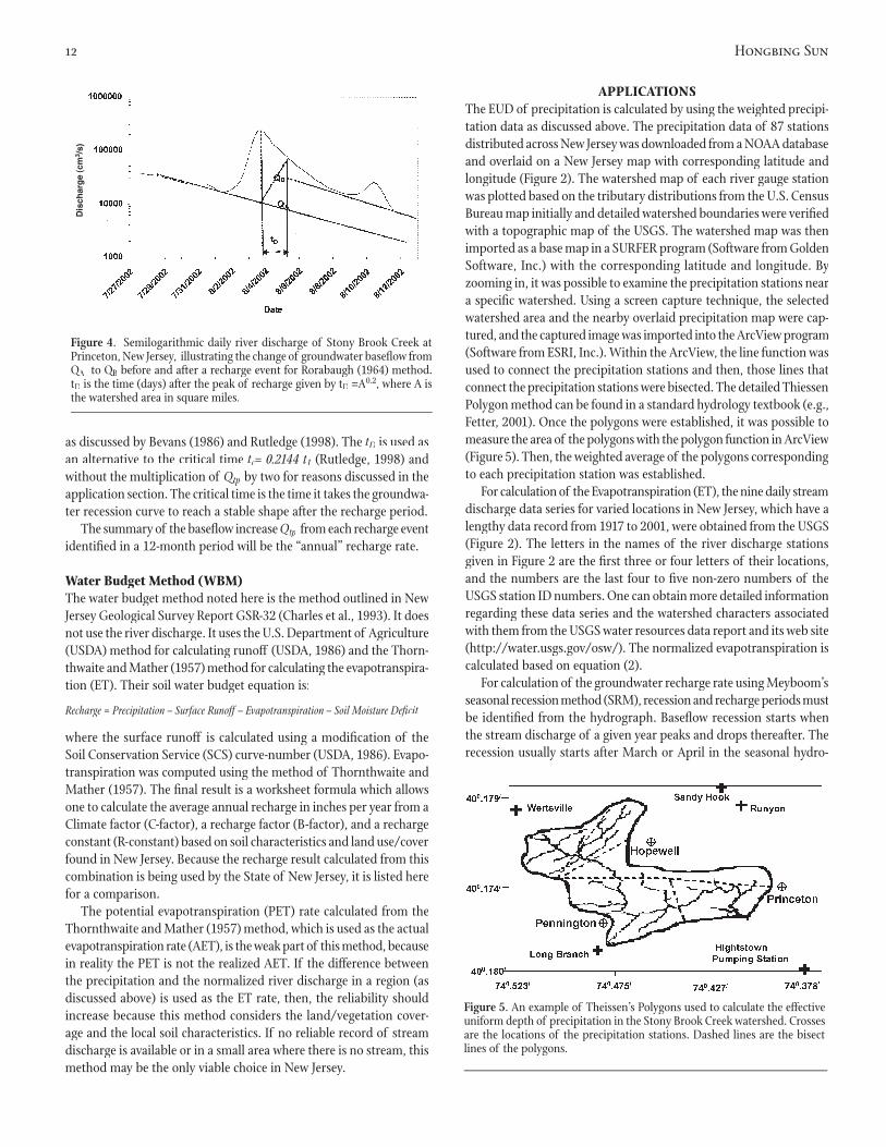
APPLICATIONSThe EUD of precipitation is calculated by using the weighted precipi-tation data as discussed above. The precipitation data of 87 stations distributed across New Jersey was downloaded from a NOAA database and overlaid on a New Jersey map with corresponding latitude and longitude (Figure 2). The watershed map of each river gauge station was plotted based on the tributary distributions from the U.S. Census Bureau map initially and detailed watershed boundaries were verifi ed with a topographic map of the USGS. The watershed map was then imported as a base map in a SURFER program (Software from Golden Software, Inc.) with the corresponding latitude and longitude. By zooming in, it was possible to examine the precipitation stations near a specifi c watershed. Using a screen capture technique, the selected watershed area and the nearby overlaid precipitation map were cap-tured, and the captured image was imported into the ArcView program (Software from ESRI, Inc.). Within the ArcView, the line function was used to connect the precipitation stations and then, those lines that connect the precipitation stations were bisected. The detailed Thiessen Polygon method can be found in a standard hydrology textbook (e.g., Fetter, 2001). Once the polygons were established, it was possible to measure the area of the polygons with the polygon function in ArcView (Figure 5). Then, the weighted average of the polygons corresponding to each precipitation station was established.

For calculation of the Evapotranspiration (ET), the nine daily stream discharge data series for varied locations in New Jersey, which have a lengthy data record from 1917 to 2001, were obtained from the USGS (Figure 2). The letters in the names of the river discharge stations given in Figure 2 are the fi rst three or four letters of their locations, and the numbers are the last four to fi ve non-zero numbers of the USGS station ID numbers. One can obtain more detailed information regarding these data series and the watershed characters associated with them from the USGS water resources data report and its web site (http://water.usgs.gov/osw/). The normalized evapotranspiration is calculated based on equation (2).

For calculation of the groundwater recharge rate using Meyboom’s seasonal recession method (SRM), recession and recharge periods must be identifi ed from the hydrograph. Basefl ow recession starts when the stream discharge of a given year peaks and drops thereafter. The recession usually starts after March or April in the seasonal hydro-

Figure 5. An example of Theissen’s Polygons used to calculate the effective uniform depth of precipitation in the Stony Brook Creek watershed. Crosses are the locations of the precipitation stations. Dashed lines are the bisect lines of the polygons.

Figure 4. Semilogarithmic daily river discharge of Stony Brook Creek at Princeton, New Jersey, illustrating the change of groundwater basefl ow from QAQAQ to QB to QB to Q before and after a recharge event for Rorabaugh (1964) method. tD is the time (days) after the peak of recharge given by tD =A0.2, where A is the watershed area in square miles.

Fate of Precipitation from Stream Discharge in New Jersey 13

Table 1. Allocations of Precipitation in New JerseyTable 1. Allocations of Precipitation in New Jersey

Table 2. Allocation Ratios of Precipitation in New JerseyTable 2. Allocation Ratios of Precipitation in New Jersey

Table 3. Comparison of Precipitation PartitionTable 3. Comparison of Precipitation Partition

14 Hongbing Sun

graph in New Jersey. The basefl ow volume of a watershed, which is equivalent to its volume of groundwater recharge, is then normalized by using the basefl ow volume divided by the total catchment area of this watershed. The runoff is the volume of river discharge minus the basefl ow volume. The calculated groundwater recharge rate is divided by the EUD of precipitation of a watershed to obtain the recharge/precipitation ratio.

The daily average river discharge has been conventionally used in the application of the SRM (Meyboom, 1961; Domenico and Schwartz, 1998; and Fetter, 2001). As illustrated in Figure 3, this method es-sentially uses the two lowest log average daily discharges to defi ne the recession line while ignoring any recharge events above the two lowest points. Apparently, the groundwater recharge estimation from the two lowest log average daily discharges can under-represent the actual groundwater recharge in the recharge season. As an alternative, a recharge rate using the monthly average river discharge is calculated (Tables 1 and 2), along with the recharge rate based on the daily river discharge. From Table 2, the average groundwater recharge calculated from the daily discharge by SRM is only 13.9% of the precipitation, which is quite lower in comparison with the data from other sources in similar climate regions (Table 3). In contrast, the recharge rate calculated from the monthly average discharges is more in-line with the result from other sources (Table 3). The small recharge events that are overestimated because discharge values are averaged monthly are offset by the large recharge events that are underestimated. In other words, the two minimum average monthly discharges are more representative of the average seasonal basefl ow trend than are the two minimum average daily discharges. The second alternative is to use a linear recession line that goes through all the daily data so that some of the data will be above the line and some of the data will be below the line to obtain a better representative value (Rutledge, 2004, personal comm.).

The recession curve displacement method (RCDM) uses the aver-age daily value to calculate each sizable individual recharge amount. Because it identifi es more sizable recharge events than merely the general trend, it yields more accurate data on the annual groundwater recharge estimation. Bevans (1986) and Rutledge (1998, 2000) gave a more detailed explanation of the RCDM. Rutledge (1998) developed a RORA program for calculating the recharge rate. However, the RORA program, which is based on Bevans (1986), asserts that the recharge rate is 2*Qtp2*Qtp2*Q of equation (8), with QAQAQ and QBQBQ extracted at the critical time tc. From Table 2, the recharge rate calculated from the RORA program (Rutledge, 1998) is about 82% of the total river discharge (the recharge/discharge ratio in the table). In three of the watersheds, the recharge rates calculated directly from RORA are larger or close to the long-term stream discharges (Tables 1 and 2). The large recharge rate can derive from the improper treatment of antecedent recession during the program execution. Because the stream discharge is run over multi-year periods, the large ground water recharge can also imply an overestimation problem of the 2*Qtp2*Qtp2*Q assertion. The average recharge/river discharge ratio of 75.2 listed by Zapecza et al. (2003), which used the RORA program for the Highlands region of New Jer-sey and New York, also tends to be high in comparison with the data from other studies (Table 3). For comparison, both the values from

direct equation (8) and the values from the RORA program, with the assertion 2*Qtp2*Qtp2*Q of equation (8) with QAQAQ and QBQBQ being extracted at the critical time tctct , are listed in Tables 1 and 2. The identifi cation of t1t1tfor multi-year data can still be obtained using the RECESS program developed by Rutledge (1998). The recharge rate using equation (8) can also be calculated from the modifi cation of the RORA program, where the recharge rates, QAQAQ and QB,QB,Q are used at time tDtDt instead of at critical time tctct .

As evident from Table 3, it is clear that there is a general agree-ment on the evapotranspiration portion of precipitation from various sources. That is, about 48 to 59% of annual precipitation (~57.25 cm or 22.54 inches) is evaporated in New Jersey on average. Ignoring the low values by the SRM using the daily discharge value, it is agreed that about 25 to 30% of the precipitation is recharged into groundwater. Results from both the SRM using the monthly discharge data and the RCDM using the daily value are comparable. About 15 to 30% of the precipitation becomes direct runoff (Figure 6).

Fluctuations apparently exist in the ratios of groundwater recharge/precipitation of a region through the years because of the variations of evapotranspiration through seasons. In addition, variations exist from regions to regions. Comparing the northern and southern parts of the state from the results of SRM based on the monthly data (except the Wallkill region for which no data are available), the average recharge rates are higher in the southern regions with 26.45% (average of F: 24.9%, E: 28.5%, 29.7%, and 22.7%) than that of the northern regions with 22.7% (average of B: 20.2%, 24.6, C: 28%, and D: 23.9% and 17%) (See Figure 2 for locations). The differences in these regional recharge rates refl ect the differences between the topography, soil, and geology between the northern and southern parts of the state.

Figure 6. Illustration of the fate of the precipitation in New Jersey. A total of 47.7% of precipitation goes to evapotranspiration, 25.4% and 26.9% of the precipitation go to recharge groundwater and runoff respectively. The numbers are averaged from SRM monthly data and RCDM data.

Fate of the precipitation in New Jersey

Fate of Precipitation from Stream Discharge in New Jersey 15

SUMMARY AND CONCLUSIONSA procedure based on the classical hydrological methods for estimating the fate of precipitation in a watershed is summarized and discussed. While the calculation of annual evapotranspiration from the river discharge is relatively straightforward, the calculation of groundwater recharge based on the basefl ow recession of a river discharge is more complicated. Alternative applications of seasonal recession and reces-sion curve displacement methods for calculating the groundwater recharge are examined. Both the SRM with monthly discharge value and the RCDM with discharge potentials extracted at time tDtDt =A0.2 can give comparable results with the existing data. Results of the calcula-tions in this paper show that about 47.7% of the annual precipitation is evapotranspired in New Jersey on average. About 25 to 30% of the precipitation recharges into groundwater. About 15 to 30% of the precipitation goes to direct runoff. Variations in the amount of runoff and basefl ow exist between the northern and southern parts of New Jersey. These variations refl ect differences in the topography and geology of the northern and southern parts of the state.

ACKNOWLEDGMENTSThe author wants to thank Albert Rutledge of USGS for his generous help with the use of the RORA program and frank discussions about the recession curve displacement method for calculating ground water recharge. The author is also grateful to Anthony Navoy of USGS for his technical assistance. The author likewise thanks Jonathan Husch of Rider University and one of the anonymous reviewers for their critical comments and editing, and Gregory Cavallo of Delaware River Basin Commission for his assistance in locating two USGS documents.

LITERATURE CITEDANDERSON, M. P. and W. W. WOESSNER. 1992. Applied Groundwater Modeling.

Simulation of Flow and Advective Transport. Academic Press, San Diego.BEVANS, H. E. 1986. Estimating stream-aquifer interactions in coal areas of

eastern Kansas by using streamfl ow records. In: S. Subitzky, (ed.), Selected Papers in the Hydrologic Sciences. U.S. Geological Survey Water-Supply Paper 2290, P. 51-64.

DOMENICO, P.A. and F.W. SCHWARTZ. 1998. Physical and Chemical Hydrogeol-ogy. 2nd edition, John Wiley & Sons, New York.nd edition, John Wiley & Sons, New York.nd

CHARLES, E. G., C. BEHROOZI, J. SCHOOLEY, and J. L. HOFFMAN. 1993. A Method of Evaluating Ground-water-Recharge Areas in New Jersey, NJ Geological Survey Report GSR-32. Trenton, New Jersey.

FETTER, C. W. 2001. Applied Hydrology. Prentice Hall, Englewood Cliff, New Jersey.

LERNER, D. N., A. S. ISSAR, and I. SIMMERS. 1990. Groundwater Recharge. A Guide to Understanding and Estimating Natural Recharge. Hannover, West Germany.

MEYBOOM, P. 1961. Estimating groundwater recharge from stream hydrographs. Journal of Geophysical Research 66: 1203-14.

NEW JERSEY WATER SUPPLY AUTHORITY. 2000. Water Budget in the Raritan River Basin. Technical Report for the Raritan Basin Watershed Management Project. Trenton, New Jersey.

PIPKIN, B.W. and D. D. TRENT. 2001. Geology and the Environment. Brooks/Cole, Belmont, California.

RORABAUGH, M. I. 1964. Estimating Changes in Bank Storage and Groundwater Contribution to Streamfl ow. International Association of Scientifi c Hydrology, Publication 63, pp.432-441.

RUTLEDGE, R.T. 1998. Computer Programs for Describing the Recession of Groundwater Discharge and for Estimating Mean Groundwater Recharge and Discharge from Streamfl ow Records-Update. USGS Water-Resource Investigations Report 98-4148. Reston, Virginia.

RUTLEDGE, R.T. 2000. Considerations for Use of the RORA Program to Estimate Groundwater Recharge from Streamfl ow Records. USGS Open-File-Report 00-156, Reston, Virginia

SLOTO, R.A. 2004. Geophydrology of the French Creek Basin and Simulated Effects of Drought and Ground-water Withdrawals, Chester County, Penn-sylvania. USGS Water-Resources Investigations Report 03-4263, New Cum-berland, Pennsylvania.

SLOTO, R.A., L. D. CECIL, and L. A. SENIOR. 1991. Hydrogeology and Ground-water Flow in the Carbonate Rocks of the Little Lehigh Creek Basin, Lehigh County, Pennsylvania. USGS Water-Resources Investigation Report 90-4076, Lemoyne, Pennsylvania.

THORNTHWAITE, C.W., and J. R. MATHER. 1957. Instructions and Tables for Computing Potential Evapotranspiration and the Water Balance. Publication 10, Laboratory of, Climatology, Centerton, New Jersey, pp.185-311.

UMA, K.O. and B.C.E. EGBOKA. 1987. Groundwater recharge from three cheap and independent methods in small watersheds of the rain forest belt of Nigeria. In Simmers, I. (ed.), Estimation of Natural Groundwater Recharge, D. Reidel Publishing Company, Boston, Massachusetts.

USDA (US Department of Agriculture). 1986. Technical Report 55 (TR-55)-Urban Hydrology for Small Watersheds (2nd ed.). Washington, D. C. 156pnd ed.). Washington, D. C. 156pnd .

VOGEL and RELF, 1993. Geohydrology and Simulation of Groundwater Flow in the Red Clay Creek Basin, Chester County, Pennsylvania and New Castle County, Delaware. USGS Water Resources Investigations Report 93-4055.Lemoyne, Pennsylvania.

ZAPECZA, O. S., D. R. RICE, and V. T., DEPAUL, 2003. New York – New Jersey Highlands Regional Study. Technical Report, USDA, Forest Service, NA-TP-04-03. Newtown Square, Pennsylvania.