REVIEW OF TERMINOLOGY

Statistics Parameters Critical Region “Obtained” test statistic “Critical” test statistic Alpha/Confidence Level

SIGNIFICANCE TESTING

Old way Find “critical value” of test statistic The point

at which the odds of finding that statistic under the null are less than alpha.

Compare your obtained test statistic with the critical test statistic. If your obtained is greater than your critical, reject the null. Odds of finding that “obtained” value are less than

alpha (5%, 1%) if the null is true.

SPSS Look at “sig” value (aka, “p” value)

Assuming the null is true, there is an X percent chance of obtaining this test statistic.

If it is less than alpha, reject null

T-TESTS

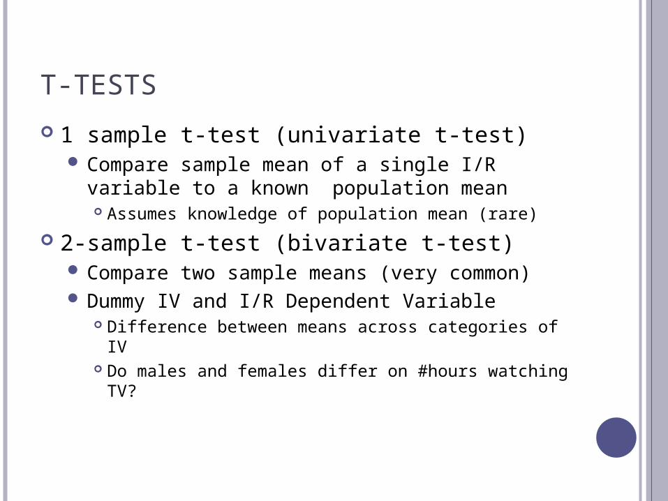
1 sample t-test (univariate t-test) Compare sample mean of a single I/R variable to

a known population mean Assumes knowledge of population mean (rare)

2-sample t-test (bivariate t-test) Compare two sample means (very common) Dummy IV and I/R Dependent Variable

Difference between means across categories of IV Do males and females differ on #hours watching TV?

THE T DISTRIBUTION

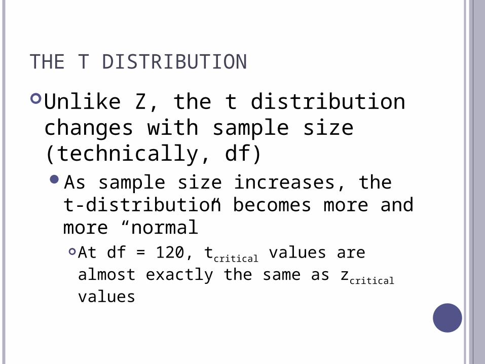
Unlike Z, the t distribution changes with sample size (technically, df)As sample size increases, the t-

distribution becomes more and more “normal”At df = 120, tcritical values are almost exactly the same as zcritical values

T AS A “TEST STATISTIC”

• All test statistics indicate how different our finding is from what is expected under null– Mean differences under null hypothesis =

0– t indicates how different our finding is from

zero• There is an exact “sig” or “p” value

associated with every value of t– SPSS generates the exact probability

associated with your obtained t

T-SCORE IS “MEANINGFUL”

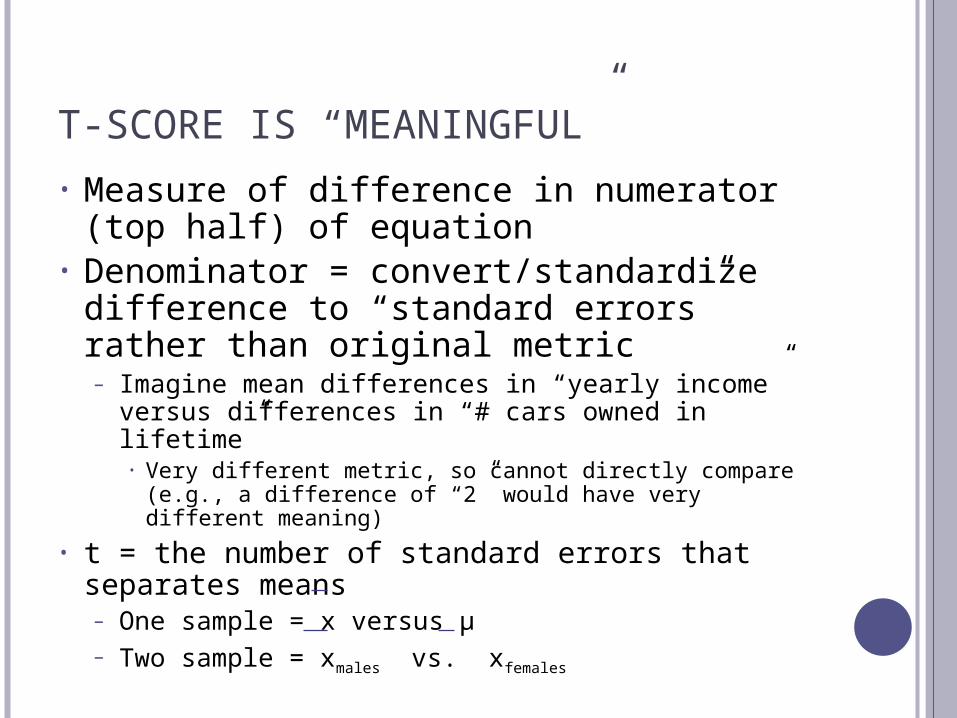
• Measure of difference in numerator (top half) of equation

• Denominator = convert/standardize difference to “standard errors” rather than original metric– Imagine mean differences in “yearly income”

versus differences in “# cars owned in lifetime”• Very different metric, so cannot directly compare (e.g.,

a difference of “2” would have very different meaning)

• t = the number of standard errors that separates means– One sample = x versus µ– Two sample = xmales vs. xfemales

T-TESTING IN SPSS

• Analyze compare means independent samples t-test– Must define categories of IV (the dummy

variable)• How were the categories numerically coded?

• Output– Group Statistics = mean values – Levine’s test

• Not real important, if significant, use t-value and sig value from “equal variances not assumed” row

– t = “tobtained” • no need to find “t-critical” as SPSS gives you “sig” or the

exact probability of obtaining the tobtained under the null

SPSS T-TEST EXAMPLE Independent Samples t Test Output:

Testing the Ho that there is no difference in GPA between white and nonwhite UMD students

Is there a difference in the sample?Group Statistics

Race N Mean Std. DeviationStd. Error

MeanGPA nonwhite 34 3.185 .4869 .0835

white 432 3.068 .5573 .0268

INTERPRETING SPSS OUTPUT Difference in GPA across Race? Obtained t value? Degrees of freedom? Obtained p value? Specific meaning of p-value? Reject null?

Independent Samples Test

Levene's Test for Equality of Variances

F Sig. t dfSig. (2-tailed)

Mean Difference

GPA Equal variances assumed

1.057 .304 1.189 464 .235 .1170

Equal variances not assumed

1.334 40.125 .190 .1170

SPSS AND 1-TAIL / 2-TAIL

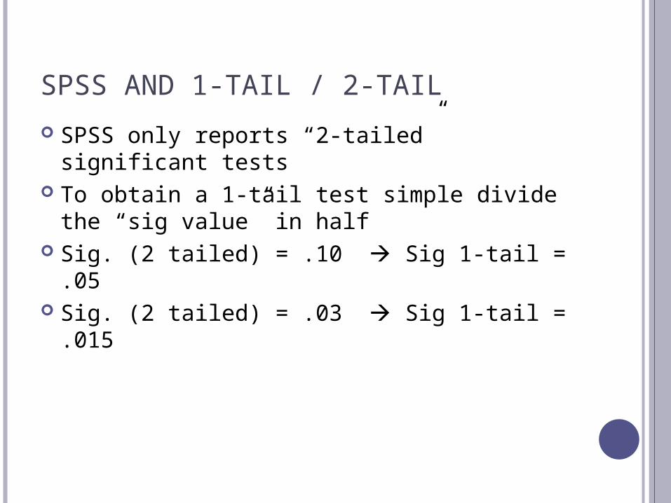
SPSS only reports “2-tailed” significant tests To obtain a 1-tail test simple divide the “sig

value” in half Sig. (2 tailed) = .10 Sig 1-tail = .05 Sig. (2 tailed) = .03 Sig 1-tail = .015

FACTORS IN THE PROBABILITY OF REJECTING H0 FOR T-TESTS

1. The size of the observed difference (produces larger t-observed)

2. The alpha level (need larger t-observed in order to reject null)

3. The use of one or two-tailed tests (two tailed tests make it harder to reject null)

4. The size of the sample (larger N produces larger t-values).

ANALYSIS OF VARIANCE

What happens if you have more than two means to compare?

IV (grouping variable) = more than two categories Examples

Risk level (low medium high) Race (white, black, native American, other)

DV Still I/R (mean)

ANOVA = F-TEST

The purpose is very similar to the t-test

HOWEVER Computes the test statistic “F” instead of “t”And does this using different logic because

you cannot calculate a single distance between three or more means.

ANOVA

Why not use multiple t-tests?Error compounds at every stage probability of making an error gets too large

F-test is therefore EXPLORATORYIndependent variable can be any level

of measurementTechnically true, but most useful if categories are limited (e.g., 3-5).

HYPOTHESIS TESTING WITH ANOVA:Different route to calculate the test statistic

2 key concepts for understanding ANOVA:SSB – between group variation (sum of squares)SSW – within group variation (sum of squares)

ANOVA compares these 2 type of varianceThe greater the SSB relative to the SSW, the more likely that the null hypothesis (of no difference among sample means) can be rejected

TERMINOLOGY CHECK

“Sum of Squares” = Sum of Squared Deviations from the Mean = (Xi - X)2

Variance = sum of squares divided by sample size = (Xi - X)2 = Mean Square

N Standard Deviation = the square root of

the variance = s

ALL INDICATE LEVEL OF “DISPERSION”

THE F RATIO Indicates the variance between the

groups, relative to variance within the groups

F = Mean square (variance) between Mean square (variance) within

Between-group variance tells us how different the groups are from each other

Within-group variance tells us how different or alike the cases are as a whole sample

ANOVA

ExampleRecidivism, measured as mean # of crimes

committed in the year following release from custody: 90 individuals randomly receive 1of the following

sentences: Prison (mean = 3.4) Split sentence: prison & probation (mean = 2.5) Probation only (mean = 2.9)

These groups have different means, but ANOVA tells you whether they are statistically significant – bigger than they would be due to chance alone

# OF NEW OFFENSES: DEMO OFBETWEEN & WITHIN GROUP VARIANCE

2.0 2.5 3.0 3.5 4.0

GREEN: PROBATION (mean = 2.9)

# OF NEW OFFENSES: DEMO OFBETWEEN & WITHIN GROUP VARIANCE

2.0 2.5 3.0 3.5 4.0

GREEN: PROBATION (mean = 2.9)BLUE: SPLIT SENTENCE (mean = 2.5)

# OF NEW OFFENSES: DEMO OFBETWEEN & WITHIN GROUP VARIANCE

2.0 2.5 3.0 3.5 4.0

GREEN: PROBATION (mean = 2.9)BLUE: SPLIT SENTENCE (mean = 2.5)RED: PRISON (mean = 3.4)

# OF NEW OFFENSES: WHAT WOULD LESS “WITHIN GROUP VARIATION” LOOK LIKE?

2.0 2.5 3.0 3.5 4.0

GREEN: PROBATION (mean = 2.9)BLUE: SPLIT SENTENCE (mean = 2.5)RED: PRISON (mean = 3.4)

ANOVA

Example, continuedDifferences (variance) between groups is also

called “explained variance” (explained by the sentence different groups received).

Differences within groups (how much individuals within the same group vary) is referred to as “unexplained variance” Differences among individuals in the same group can’t

be explained by the different “treatment” (e.g., type of sentence)

F STATISTIC

When there is more within-group variance than between-group variance, we are essentially saying that there is more unexplained than explained variance

In this situation, we always fail to reject the null hypothesis

This is the reason the F(critical) table (Healey Appendix D) has no values <1

SPSS EXAMPLE Example:

1994 county-level data (N=295) Sentencing outcomes (prison versus other [jail or

noncustodial sanction]) for convicted felons Breakdown of counties by region:

REGION

67 22.7 22.7 22.7

43 14.6 14.6 37.3

140 47.5 47.5 84.7

45 15.3 15.3 100.0

295 100.0 100.0

MW

NE

S

W

Total

ValidFrequency Percent Valid Percent

CumulativePercent

SPSS EXAMPLE

Question: Is there a regional difference in the percentage of felons receiving a prison sentence? Null hypothesis (H0):

There is no difference across regions in the mean percentage of felons receiving a prison sentence.

Mean percents by region:

Report

TOT_PRIS

44.033 66 21.6080

45.917 43 17.9080

58.236 140 27.0249

28.574 44 16.3751

48.775 293 25.4541

REGIONMW

NE

S

W

Total

Mean N Std. Deviation

SPSS EXAMPLEThese results show that we can reject the null

hypothesis that there is no regional difference among the 4 sample means The differences between the samples are large enough

to reject Ho The F statistic tells you there is almost 20 X more between

group variance than within group variance The number under “Sig.” is the exact probability of obtaining this F by chance

ANOVA

TOT_PRIS

32323.544 3 10774.515 19.850 .000

156866.3 289 542.790

189189.8 292

Between Groups

Within Groups

Total

Sum ofSquares df Mean Square F Sig.

A.K.A. “VARIANCE”

ANOVA: POST HOC TESTS

The ANOVA test is exploratoryONLY tells you there are sig. differences between means, but not WHICH means

Post hoc (“after the fact”) Use when F statistic is significantRun in SPSS to determine which means (of the 3+) are significantly different

OUTPUT: POST HOC TEST This post hoc test shows that 5 of the 6 mean differences

are statistically significant (at the alpha =.05 level) (numbers with same colors highlight duplicate comparisons)

p value (info under in “Sig.” column) tells us whether the difference between a given pair of means is statistically significant

Multiple Comparisons

Dependent Variable: TOT_PRIS

Scheffe

-1.884 4.5659 .982 -14.723 10.956

-14.203* 3.4787 .001 -23.985 -4.421

15.460* 4.5343 .010 2.709 28.210

1.884 4.5659 .982 -10.956 14.723

-12.319* 4.0620 .028 -23.742 -.897

17.344* 4.9959 .008 3.295 31.392

14.203* 3.4787 .001 4.421 23.985

12.319* 4.0620 .028 .897 23.742

29.663* 4.0266 .000 18.340 40.986

-15.460* 4.5343 .010 -28.210 -2.709

-17.344* 4.9959 .008 -31.392 -3.295

-29.663* 4.0266 .000 -40.986 -18.340

(J) REG_NUMNE

S

W

MW

S

W

MW

NE

W

MW

NE

S

(I) REG_NUMMW

NE

S

W

MeanDifference

(I-J) Std. Error Sig. Lower Bound Upper Bound

95% Confidence Interval

The mean difference is significant at the .05 level.*.

ANOVA IN SPSSSTEPS TO GET THE CORRECT OUTPUT…

ANALYZE COMPARE MEANS ONE-WAY ANOVA

INSERT…INDEPENDENT VARIABLE IN BOX LABELED “FACTOR:”

DEPENDENT VARIABLE IN THE BOX LABELED “DEPENDENT LIST:”

CLICK ON “POST HOC” AND CHOOSE “LSD”CLICK ON “OPTIONS” AND CHOOSE “DESCRIPTIVE”

YOU CAN IGNORE THE LAST TABLE (HEADED “Homogenous Subsets”) THAT THIS PROCEDURE WILL GIVE YOU