qbase+ manual
TRANSCRIPT

Manual

Copyright 2010-2017 qbase+ manual (rev 2017-04-24)
www.qbaseplus.com 2 / 93
Table of contents
Table of contents
Installation
First time users
Using a basic or premium license
Advanced memory settings
General Definitions
Overview of qPCR workflow
The analysis wizard in qbase+
Steps in qbase+
Getting started
Expert mode
Menu and command bar
Workspace
Projects
Experiments
Runs
Data exchange
Projects and experiments
Runs
Samples and targets
Project and experiment annotation
Run annotation
Sample annotation
Target annotation
Renaming and clean-up
Calculation parameters
Quality control settings
The inter-run calibration concept
Inter-run calibration in qbase+
Quality control and results
Use one default amplification efficiency
Use target specific amplification efficiencies
Make amplification efficiencies run specific
Copyright 2010-2017 qbase+ manual (rev 2017-04-24)
www.qbaseplus.com 3 / 93
Technical replicates
Positive and negative controls
Stability of reference targets
Sample quality control
Target bar charts
Multi-target bar chart
Correlation plot
Result table
Using the statistical wizard
Specify the goal of your analysis
Statistical result table and conditions of use
Statistical background
Exports
Export Amplification Efficiencies
Export Experiment
Export Normalization Factors
Export Project
Export Raw Data Table (RQ)
Export Reference Target Stabilities
Export Replicates (Cq)
Export Results Table (CNRQ)
Export Samples
Export Targets
Export Statistics Results
Export Figures
Special applications
Import run data in a new empty experiment
Selection of normalization strategy and reference genes
Interpret geNorm results
Import run data in a new empty experiment
Define calculation parameters
Define control samples
Select reference genes
Quality control
Copy number analysis results
Support
What are the hard and software requirements for running qbase+?
Can I analyze data from my qPCR instrument in qbase+?
What are the basic calculations in qbase+?
What is the meaning of CNRQ value in the result table?
Where is the calculate button?
How do I save the changes to my experiments?
How is PCR efficiency calculated and used for relative quantification?

Copyright 2010-2017 qbase+ manual (rev 2017-04-24)
www.qbaseplus.com 4 / 93
How to interpret the target bar chart?
How does qbase+ deal with replicates?
What is inter-run calibration and how does it work?
When do I need IRC?
How to flag bad technical replicates based on a standard deviation threshold?
How to exclude PCR replicates that do not meet quality control criteria?
Why does qbase+ ask to log transform the data when exporting the results table?
Does the statistical wizard perform a log transformation?
Where does qbase+ save my data?
What is the difference between Reference target stability and geNorm?
What is the difference between "M" and "geNorm M" in qbase+? How are the calculations
different?
What to expect when performing a geNorm analysis in qbase+?
Copyright 2010-2017 qbase+ manual (rev 2017-04-24)
www.qbaseplus.com 5 / 93
qbase+ is software developed by Biogazelle for analysis of quantitative PCR data. It
is based on the geNorm (Vandesompele et al., Genome Biology, 2002) and qBase
technology (Hellemans et al., Genome Biology, 2007) from Ghent University.
The software runs on a local computer with either Microsoft Windows, Apple OS X
or Linux operating system and is compatible with virtually all qPCR instruments. The
first version was released in March 2008, with frequent updates; the latest version
is 3.1.
The software is intended for relative quantification (whereby different
normalization strategies developed by the Biogazelle founders are available) and
for gene copy number analysis. The geNorm module for determining the expression
stability of candidate references and the optimal number of reference genes for
accurate normalization is a much-improved version of the original algorithm. The
implemented analysis wizard allows the straightfoward step-by-step analysis of
every qPCR experiment. The statistical wizard built into qbase+ makes it easy for
any biologist to come to expert results and reliable conclusions.
I’m convinced using qbase+ will lead to more reliable results in a shorter period of
time!
Jan Hellemans, co-founder and CEO

Copyright 2010-2017 qbase+ manual (rev 2017-04-24)
www.qbaseplus.com 6 / 93
Installation and licensing
Installation
Different versions of qbase+ are available for installation. It is import to download
the version matching your operating system (Windows, Mac or Linux) and bitness
(32-bit or 64-bit).If compatible with your system, we advise to select the 64-bit
version as it allows the use of larger amounts of memory to support analysis of very
large experiments.
qbase+ requires JAVA to be installed on your system. Many systems already have
JAVA installed. Not every version of JAVA would be suitable. It needs to be a 32-bit
JAVA for 32-bit versions of qbase+ and a 64-bit JAVA for 64-bit versions of qbase+.
qbase+ does require JAVA 1.8 or more recent. On Windows, a suitable version of JAVA
will be co-installed as part of the installation procedure of qbase+.
To install qbase+ on Windows and Mac, double click on the downloaded installer
and follow the instructions (Figure 1). The procedure for Linux is somewhat
different. Instead of using an installer, the downloaded file needs to be unzipped
and moved to an appropriate location. In addition, the execution bit needs to be set
before qbase+ can be launched.
Figure 1: qbase+ setup wizard
Copyright 2010-2017 qbase+ manual (rev 2017-04-24)
www.qbaseplus.com 7 / 93
First time users
We offer a trial version of qbase+ for evaluation purposes. For a period of two
weeks, all premium functionalities will be available.
Every installation of qbase+ includes various carefully selected and representative
data sets for:
• gene expression analysis
• microRNA profiling
• geNorm pilot reference gene stability analysis
• gene copy number analysis
• ChIP-qPCR
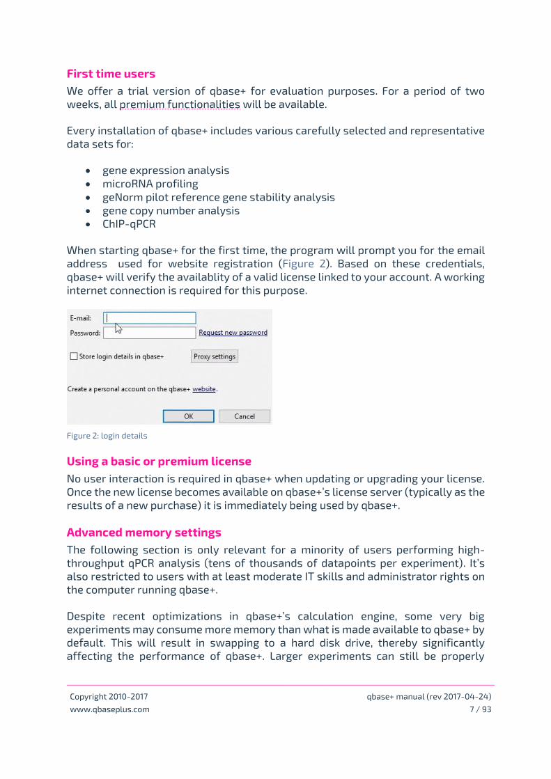
When starting qbase+ for the first time, the program will prompt you for the email
address used for website registration (Figure 2). Based on these credentials,
qbase+ will verify the availablity of a valid license linked to your account. A working
internet connection is required for this purpose.
Figure 2: login details
Using a basic or premium license
No user interaction is required in qbase+ when updating or upgrading your license.
Once the new license becomes available on qbase+’s license server (typically as the
results of a new purchase) it is immediately being used by qbase+.
Advanced memory settings
The following section is only relevant for a minority of users performing high-
throughput qPCR analysis (tens of thousands of datapoints per experiment). It’s
also restricted to users with at least moderate IT skills and administrator rights on
the computer running qbase+.
Despite recent optimizations in qbase+’s calculation engine, some very big
experiments may consume more memory than what is made available to qbase+ by
default. This will result in swapping to a hard disk drive, thereby significantly
affecting the performance of qbase+. Larger experiments can still be properly
Copyright 2010-2017 qbase+ manual (rev 2017-04-24)
www.qbaseplus.com 8 / 93
processed by changeing the amount of memory that may be allocated to qbase+ in
a so called ini-file.
For both Linux, Windows and Mac, we recommend to modify the ‘qbase+.ini’ file to
take advantage of more RAM memory (limited to around 1.5 Gb in a 32-bit
environment). This file can be found in the installation directory of qbase+,
‘C:\Program Files\qbase+\’ or ‘C:\Program Files (x86)\qbase+\’ on a Windows
system for the 64 and 32 bit versions, respectively. To find the settings file on a Mac
system, right click (or CTRL-click) on the qbase+ application, choose 'Show Package
Contents' and Browse to Contents -> MacOS.
Open the file with a text editor, locate the line with “-Xmx1024m” and modify the
number and unit depending on the amount of RAM available (e.g. “-Xmx3g” on a
system with 4 Gb RAM, or “-Xmx7g” on a system with 8 Gb of RAM; general guideline:
1 Gb (g) less than the amount of RAM in Gb; make sure there is no space in between
Xmx and the number). These settings need to be updated with every new
installation of qbase+. On most systems, administrator rights are required to update
these settings.
Copyright 2010-2017 qbase+ manual (rev 2017-04-24)
www.qbaseplus.com 9 / 93
Definitions and concepts
General Definitions
Target
The generic term used for the DNA sequence to be quantified. It typically refers
to a gene, but could also refer to a specific transcript or a genomic locus. Two
target types are recognized: targets of interest and reference targets
Cq value
Cq is the MIQE standard name for Ct (cycle threshold), Cp (crossing point), or
other instrument specific quantification value name.
Run
Runs are collections of qPCR data coming from a single plate, array, rotor or chip
(depending on the instrument being used).
Experiment
The set of data (stored in one or multiple runs), annotations and settings used
for qPCR data analysis.
Project
Logical groups of related experiments.
Inter-run calibration
A calculation procedure to detect and remove inter-run variation.
Sample
In qbase+, a sample is defined as the nucleic acid dilution on which the qPCR
measurement is performed. According to this definition, a serial dilution made
from a single RT reaction or DNA sample would consist of different sample
names.
RDML
A universal, open and XML based data format for the exchange of qPCR data,
recommended by the MIQE guidelines.
Reference target
The targets that will be used to normalize the qPCR data. In the context of gene
expression analysis, this target type used to be referred to as housekeeping
gene.
Copyright 2010-2017 qbase+ manual (rev 2017-04-24)
www.qbaseplus.com 10 / 93
geNorm
The algorithm developed by Biogazelle co-founder prof. Jo Vandesompele
(Genome Biology, 2002) to determine the expression stability of selected
(candidate) reference targets. It can be used in geNorm pilot studies to identify
the optimal set of reference genes to be used in follow up studies, or later on to
verify the expression stability of selected reference targets.
Sample property
Two types of sample properties are used in qbase+. There is a set of predefined
sample properties such as sample name, sample type and quantity. Custom
sample properties can be added to link (usally annotation) information to
samples. For each sample, a sample property value can be entered. For example,
the sample property ‘gender’ may have sample property values ‘male’ and
‘female’.
Normalization
Normalization is the procedure by which technical sample specific variation (e.g.
differences in total amount of cDNA) is corrected for. Normalization is typically
performed by means of reference genes, but alternative approaches are
available.
Result scaling
The results of a relative quantification analysis do not have a particular scale.
Because of this they can be multiplied (or devided) by a common factor. This
process will alter the actual values, but not the sample to sample relationships
(i.e. the fold changes). It does not alter the results but may facilitate
interpretation, for example by making all results relative to a control sample.
Workspace
The workspace is the central location in which qbase+ stores all its information:
data, annotation and settings.

Copyright 2010-2017 qbase+ manual (rev 2017-04-24)
www.qbaseplus.com 11 / 93
Overview of qPCR workflow
Where does qbase+ fit in the qPCR workflow?
Figure 3: Researchers spent a considerable amount of time in preparing samples, optimizing assays and
setting up the actual experiments. Data analysis is far too often an underestimated step in the qPCR workflow.
qbase+ is a reliable, easy, fast and flexible data analysis platform, outcompeting the time-consuming,
errorprone and tradional way of doing calculations.
Copyright 2010-2017 qbase+ manual (rev 2017-04-24)
www.qbaseplus.com 12 / 93
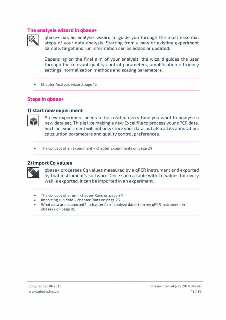
The analysis wizard in qbase+
qbase+ has an analysis wizard to guide you through the most essential
steps of your data analysis. Starting from a new or existing experiment
sample, target and run information can be added or updated.
Depending on the final aim of your analysis, the wizard guides the user
through the relevant quality control parameters, amplification efficiency
settings, normalisation methods and scaling parameters.
• Chapter Analysis wizard page 16
Steps in qbase+
1) start new experiment
A new experiment needs to be created every time you want to analyse a
new data set. This is like making a new Excel file to process your qPCR data.
Such an experiment will not only store your data, but also all its annotation,
calculation parameters and quality control preferences.
• The concept of an experiment – chapter Experiments on page 24
2) import Cq values
qbase+ processes Cq values measured by a qPCR instrument and exported
by that instrument’s software. Once such a table with Cq values for every
well is exported, it can be imported in an experiment.
• The concept of a run – chapter Runs on page 24
• Importing run data – chapter Runs on page 26
• What data are supported? – chapter Can I analyze data from my qPCR instrument in
qbase+? on page 85

Copyright 2010-2017 qbase+ manual (rev 2017-04-24)
www.qbaseplus.com 13 / 93
3) add / review sample and target naming
Runs need to be properly annotated before experiments can be analyzed.
Not only will your data be meaningless without annotation, it is simply
essential for qbase+ to start any calculations.
• Appoint sample and target names – chapter Run annotation page 33
• Creating new samples – chapter Sample annotation page 35
• Creating new targets – chapter Target annotation page 38
• Apply/copy run layouts – chapter Run annotation page 34
4) add extra sample info
Adding extra sample information will allow better graphical representation
of data (e.g. sample groups), statistical analysis of data, etc. There are three
ways by which sample information can be provided to qbase+:
1. as part of the import of a run
2. by manually adding a sample
3. by importing a sample list.
• Creating new samples – chapter Sample annotation page 35
• Sample properties – chapter Sample annotation page 36
• Custom sample properties – chapter Sample annotation page 37
5) adjust calculation parameters
Four types of parameters can be defined allowing the most appropriate
calculations for your experimental set-up:
1. the type of amplification efficiency correction
2. the most appropriate normalization method
3. the method to calculate average Cq values
4. the target scaling mode.
• Calculation parameters – chapter Calculation parameters and quality control settings page
41
• amplification efficiency – chapter PCR efficiency correction page 50
• How is PCR efficiency calculated and used for relative quantification? – chapter FAQ page
87

Copyright 2010-2017 qbase+ manual (rev 2017-04-24)
www.qbaseplus.com 14 / 93
6) adjust quality control settings
Quality control is an important aspect of qbase+. By adjusting the quality
control settings you will be able to estimate the quality of the data and/or
define criteria for automatic exclusion of certain data points.
• Quality control settings – chapter Calculation parameters and quality control settings page
43
• How to flag bad technical replicates based on a standard deviation threshold? – chapter
FAQ page 90
• How to exclude PCR replicates that do not meet quality control criteria? – chapter FAQ page
90
7) perform quality control
qbase+ contains several types of quality control that can be accessed after
adjusting the appropriate settings, including technical replicates, positive
and negative controls, stability of reference targets and sample quality
control.
• Technical replicates – chapter Quality controls page 53
• Positive and negative controls – chapter Quality controls page 55
• Stability of reference targets – chapter Quality controls page 56
• Sample quality control – chapter Quality controls page 57
(8) perform inter-run calibration
Inter-run calibration (IRC) is a calculation procedure to detect and remove
(often underestimated) inter-run variation. These calculations are typically
needed whenever samples need to be compared that are measured in
different runs.
• When do I need IRC? – chapter FAQ page 89
• The inter-run calibration concept – chapter Inter-run calibration page 45 and chapter FAQ
page 89
• Inter-run calibration in qbase+ – chapter Inter-run calibration page 47

Copyright 2010-2017 qbase+ manual (rev 2017-04-24)
www.qbaseplus.com 15 / 93
9) inspect results
qbase+ offers several possibilities to visualise qPCR experiment results.
Depending on your needs you can inspect commonly used bar charts,
correlation plots and/or results tables. Dedicates analysis modules allow
you to perform a geNorm analysis (including automated interpretation),
statistical analysis (see further) or copy number analysis.
• Target bar charts – chapter Bar charts, correlation plots and results tables page 58
• How to interpret the target bar chart?– chapter FAQ page 88
• Multi-target bar chart – chapter Bar charts, correlation plots and results tables page 60
• Correlation plot – chapter Bar charts, correlation plots and results tables plot page 61
• Result table – chapter Bar charts, correlation plots and results tables page 62
• What is the meaning of CNRQ value in the result table? – chapter FAQ page 86
• Why does qbase+ ask to log transform the data when exporting the results table?–
chapter FAQ page 90
• Special application: geNorm – chapter geNorm page 76
• What is the difference between Reference target stability and geNorm?– chapter FAQ page
91
• What is the difference between "M" and "geNorm M" in qbase+? How are the calculations
different? – chapter FAQ page 92
• What to expect when performing a geNorm analysis in qbase+? – chapter FAQ page 92
• Special application: copy number analysis– chapter Copy number analysis page 82
• Export Datasets and Tables – chapter Exports page 73
10) perform statistical analysis
qbase+ has a built-in intuitive statistical wizard to perform commonly used
statistical tests on the results that are calculated in a single experiment.
The stat module is specifically tailored towards the typical needs of
biologists performing qPCR analysis.
• Using the statistical wizard– chapter Statistics page 62
• Specify the goal of your analysis – chapter Statistics page 63
• Statistical result table and conditions of use – chapter Statistics page 67
• Statistical background– chapter Statistics page 70
• Does the statistical wizard perform a log transformation? – chapter FAQ page 91
Copyright 2010-2017 qbase+ manual (rev 2017-04-24)
www.qbaseplus.com 16 / 93
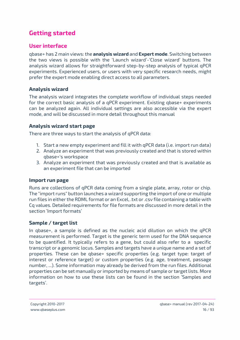
Getting started
User interface
qbase+ has 2 main views: the analysis wizard and Expert mode. Switching between
the two views is possible with the ‘Launch wizard’-‘Close wizard’ buttons. The
analysis wizard allows for straightforward step-by-step analysis of typical qPCR
experiments. Experienced users, or users with very specific research needs, might
prefer the expert mode enabling direct access to all parameters.
Analysis wizard
The analysis wizard integrates the complete workflow of individual steps needed
for the correct basic analysis of a qPCR experiment. Existing qbase+ experiments
can be analyzed again. All individual settings are also accessible via the expert
mode, and will be discussed in more detail throughout this manual
Analysis wizard start page
There are three ways to start the analysis of qPCR data:
1. Start a new empty experiment and fill it with qPCR data (i.e. import run data)
2. Analyze an experiment that was previously created and that is stored within
qbase+'s workspace
3. Analyze an experiment that was previously created and that is available as
an experiment file that can be imported
Import run page
Runs are collections of qPCR data coming from a single plate, array, rotor or chip.
The "import runs" button launches a wizard supporting the import of one or multiple
run files in either the RDML format or an Excel, .txt or .csv file containing a table with
Cq values. Detailed requirements for file formats are discussed in more detail in the
section ’Import formats’
Sample / target list
In qbase+, a sample is defined as the nucleic acid dilution on which the qPCR
measurement is performed. Target is the generic term used for the DNA sequence
to be quantified. It typically refers to a gene, but could also refer to a specific
transcript or a genomic locus. Samples and targets have a unique name and a set of
properties. These can be qbase+ specific properties (e.g. target type: target of
interest or reference target) or custom properties (e.g. age, treatment, passage
number, ...). Some information may already be derived from the run files. Additional
properties can be set manually or imported by means of sample or target lists. More
information on how to use these lists can be found in the section ’Samples and
targets’.
Copyright 2010-2017 qbase+ manual (rev 2017-04-24)
www.qbaseplus.com 17 / 93
Run annotation
Every datapoint (well) should be annotated with a sample and target name. This
information may be derived from the run files if they were properly annotated in the
qPCR instrument software. The run annotation can be reviewed, corrected and
completed by manually editing run annotation. In cases where runs have the same
layout (for either samples or targets) as a previously annotated run, that layout can
simply be copied from the annotated run to the unannotated run. Detailed
information can be found in the chapter ’Annotation’
Aim
Different types of experiments require different settings and different analyses. By
selecting the proper analysis type, qbase+ will only show the relevant settings.
Experienced users, or users with very specific research needs (e.g. ChIP-qPCR) may
exit the wizard and continue the analysis in the fully flexible Expert view. Again,
more information on all different settings will be covered throughout the manual.
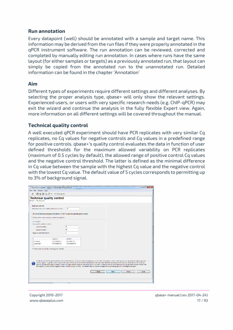
Technical quality control
A well executed qPCR experiment should have PCR replicates with very similar Cq
replicates, no Cq values for negative controls and Cq values in a predefined range
for positive controls. qbase+'s quality control evaluates the data in function of user
defined thresholds for the maximum allowed variability on PCR replicates
(maximum of 0.5 cycles by default), the allowed range of positive control Cq values
and the negative control threshold. The latter is defined as the minimal difference
in Cq value between the sample with the highest Cq value and the negative control
with the lowest Cq value. The default value of 5 cycles corresponds to permitting up
to 3% of background signal.

Copyright 2010-2017 qbase+ manual (rev 2017-04-24)
www.qbaseplus.com 18 / 93
Amplification efficiencies
The basic formula for relative quantification (RQ=2^ddCq) assumes 100%
amplification efficiency (E=2). More advanced methods correct for variable, assay
specific amplification efficiencies. These efficiencies can be calculated from
standard curves included in the experiment, or manually provided in case they were
determined before.
Normalization method
Normalization is the procedure to correct for technical variations in total cDNA
concentrations so as to distinguish samples with upregulated genes from samples
that merely have the same expression level with a higher cDNA concentration.
Several methods are available to correct for this type of variation. Normalization
based on the measurement of one or more reference (historically referred to as
housekeeping) genes is the most common option. For screening studies including a
large number of genes, global mean normalization is a valuable alternative.
Alternatively, for specific study types, users can provide custom normalization
factors such as for example the cell count. When normalizing with multiple
reference genes, the reference target stability values (M and CV) offer a measure
for the suitability of the selected reference genes for proper normalization. Good
reference genes have an M < 0.5 while M values up to 1 are acceptable for more
difficult samples.
Scaling
By default qbase+ results are scaled to the average across all unknown samples per
target. Relative quantities can be scaled arbitrarily, as long as the same scaling is
applied to all samples. Rescaling will alter the relative quantity values, but not the
relative fold changes in expression levels between samples. Rescaling is often used
to facilitate interpretation of results, e.g. by setting the expression of a control
sample or group of reference samples to 1 which makes all results relative to that
sample or sample group.
Analysis
From this page you might visually inspect the results, export the results for
downstream processing outside qbase+ or start a wizard to guide you through the
statistical interpretation of the results.

Copyright 2010-2017 qbase+ manual (rev 2017-04-24)
www.qbaseplus.com 19 / 93
Expert mode
The expert mode consists of three main windows (Figure 4): the project explorer
(left window), the main window (upper right window) and the notification window
(lower right window). The project explorer allows users to browse to the
information they want to open in the main window, whereas the notification
window contains tabs with information on alerts and program errors.
Figure 4: Three main windows in the expert mode
Project explorer
The project explorer is a hierarchical data organizer that allows users to navigate
through the experiments, settings and results. The elements in the project explorer
tree can be opened by double-clicking, or by selecting 'open' from the context menu
(this menu appears when clicking the right mouse button after placing the cursor
on top of the item). This window can be minimized to get more screen space by
clicking (-) in the upper right corner of the project explorer window, or by making
use of the context menu ('Minimize') when right-clicking on the tab. The 'always on'
situation can be restored by clicking ( ). An alternative way of working is to display
the project explorer whenever it is needed, and to have it hidden otherwise. This can
be achieved by clicking ( ); as soon as an item of the main window is selected, the
project explorer disappears.
The width of the project explorer can be controlled by moving the mouse on the
border between the project explorer and the main window (after which the pointing
arrow becomes a horizontal arrow), followed by dragging the border.
Copyright 2010-2017 qbase+ manual (rev 2017-04-24)
www.qbaseplus.com 20 / 93
Main window
When an item is opened from the project explorer, it will show up in the main
window. Double-clicking a tab will maximize this window, and the situation can be
restored by double-clicking the tab again. As an alternative, ( ) and ( ) can be used,
respectively.
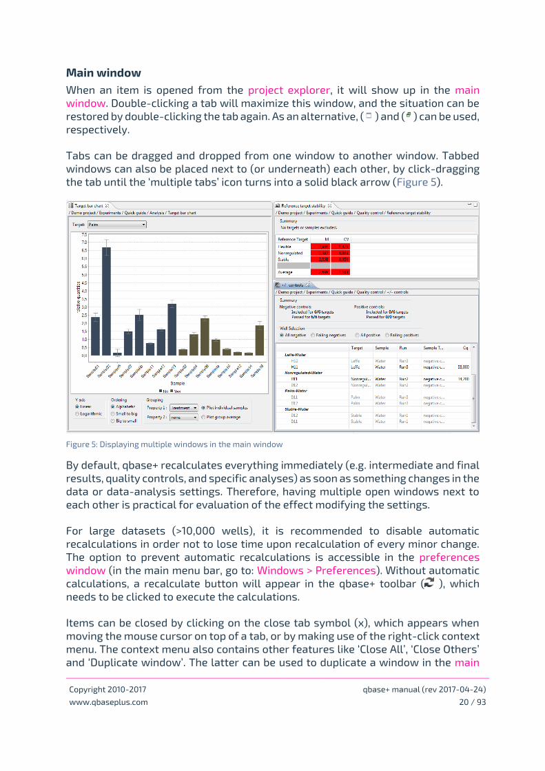
Tabs can be dragged and dropped from one window to another window. Tabbed
windows can also be placed next to (or underneath) each other, by click-dragging
the tab until the ‘multiple tabs’ icon turns into a solid black arrow (Figure 5).
Figure 5: Displaying multiple windows in the main window
By default, qbase+ recalculates everything immediately (e.g. intermediate and final
results, quality controls, and specific analyses) as soon as something changes in the
data or data-analysis settings. Therefore, having multiple open windows next to
each other is practical for evaluation of the effect modifying the settings.
For large datasets (>10,000 wells), it is recommended to disable automatic
recalculations in order not to lose time upon recalculation of every minor change.
The option to prevent automatic recalculations is accessible in the preferences
window (in the main menu bar, go to: Windows > Preferences). Without automatic
calculations, a recalculate button will appear in the qbase+ toolbar ( ), which
needs to be clicked to execute the calculations.
Items can be closed by clicking on the close tab symbol (x), which appears when
moving the mouse cursor on top of a tab, or by making use of the right-click context
menu. The context menu also contains other features like ‘Close All’, ‘Close Others’
and ‘Duplicate window’. The latter can be used to duplicate a window in the main
Copyright 2010-2017 qbase+ manual (rev 2017-04-24)
www.qbaseplus.com 21 / 93
window. Just like the project explorer, the main window can be minimized to get
more screen space.
The header of each tab contains a path, describing what is being displayed and the
position within the project explorer. This information may be essential to allow for
proper identification of results, e.g. when bar charts for the same target in two
different experiments are shown side by side.
Notification window
The notification window informs about the progress of calculation intensive steps
and the occurrence of program warnings and errors. Several items (alerts, progress
view, error log) can be added to this window (in the main menu bar, go to: Windows
> Show View).
The alert window gives clues on potential issue with experiment design or data-
analysis, e.g. no reference targets are appointed, targets are spread across runs
(necessitating inter-run calibration), technical PCR replicates are spread across
runs (not compatible with inter-run calibration), etc. By inspecting the Alert
window, many problems can be quickly identified.
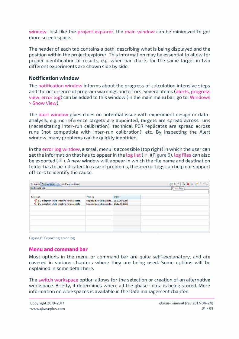
In the error log window, a small menu is accessible (top right) in which the user can
set the information that has to appear in the log list ( )(Figure 6). log files can also
be exported ( ). A new window will appear in which the file name and destination
folder has to be indicated. In case of problems, these error logs can help our support
officers to identify the cause.
Figure 6: Exporting error log
Menu and command bar
Most options in the menu or command bar are quite self-explanatory, and are
covered in various chapters where they are being used. Some options will be
explained in some detail here.
The switch workspace option allows for the selection or creation of an alternative
workspace. Briefly, it determines where all the qbase+ data is being stored. More
information on workspaces is available in the Data management chapter.

Copyright 2010-2017 qbase+ manual (rev 2017-04-24)
www.qbaseplus.com 22 / 93
Calculations
By default, qbase+ will recalculate results with each change of data, annotation or
settings. This is convenient for typically sized experiments, but may lead to slow
performance in high throughput experiments. The size at which automatic
recalculation becomes more a burden than a blessing depends on the experiment
designs, calculation settings and computer performance. Any recent computer (less
than 3 years) should be able to deal with experiments of up to ten 384-well plates
without hick-ups or recalculation delays.
For larger experiments or older computers, it may be required to turn off automatic
recalculation. When doing so, a ‘recalculate’ button is added to the command bar. It
needs to be clicked whenever changes need to take effect. This includes opening of
an experiment.
General
qbase+ allows the analysis of multiple experiments in parallel. This may be
convenient for the comparison of results. However, it may also cause confusion to
some users or slow down qbase+ when multiple large datasets are opened in
parallel. Users can set the appropriate behavior when opening another experiment
according to their needs and preferences.
Each window contains a descriptive path on the top, so you know to what
experiment the window pertains. Because of this, the option is provided to include
this path on chart prints.
Show sample in charts
Depending on their sample type, certain samples may be excluded from charts to
avoid cluttered and absurdly scaled charts. By default, unknown samples (of
interest) and positive controls will be shown. Standard (curve) samples and
negative controls (all types) will not be shown. These defaults can be changed in
this window, and overruled by making sample specific ‘sample visibility’ settings
(Figure 7).
Figure 7: Preferences for sample visualization
Copyright 2010-2017 qbase+ manual (rev 2017-04-24)
www.qbaseplus.com 23 / 93
Startup and shutdown
By default, qbase+ uses a single workspace. Advanced users that want to switch
between workspaces may use the option to have qbase+ ask for the workspace to
be used at startup.
The analysis wizard is launched when starting qbase+. Unchecking this option will
launch qbase+ with the user interface of the three main windows.
Data management
qbase+ stores all its data in a global workspace, obviating the need to deal with
storing and updating individual experiment files. Within this workspace, data and
settings are hierarchically organized into projects, experiment and runs.
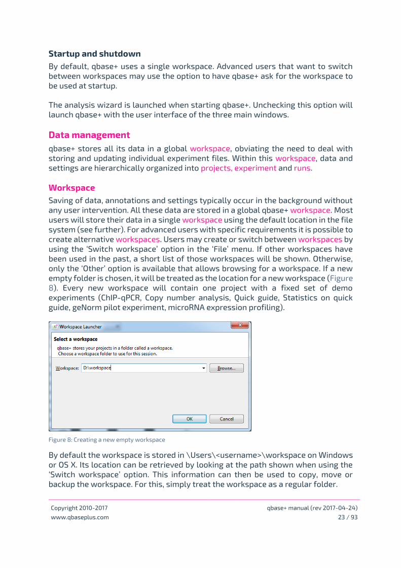
Workspace
Saving of data, annotations and settings typically occur in the background without
any user intervention. All these data are stored in a global qbase+ workspace. Most
users will store their data in a single workspace using the default location in the file
system (see further). For advanced users with specific requirements it is possible to
create alternative workspaces. Users may create or switch between workspaces by
using the ‘Switch workspace’ option in the ‘File’ menu. If other workspaces have
been used in the past, a short list of those workspaces will be shown. Otherwise,
only the ‘Other’ option is available that allows browsing for a workspace. If a new
empty folder is chosen, it will be treated as the location for a new workspace (Figure
8). Every new workspace will contain one project with a fixed set of demo
experiments (ChIP-qPCR, Copy number analysis, Quick guide, Statistics on quick
guide, geNorm pilot experiment, microRNA expression profiling).
Figure 8: Creating a new empty workspace
By default the workspace is stored in \Users\<username>\workspace on Windows
or OS X. Its location can be retrieved by looking at the path shown when using the
‘Switch workspace’ option. This information can then be used to copy, move or
backup the workspace. For this, simply treat the workspace as a regular folder.
Copyright 2010-2017 qbase+ manual (rev 2017-04-24)
www.qbaseplus.com 24 / 93
It is possible to store the workspace on a network drive or in the cloud (e.g. on
Dropbox). In view of the continuous data access that is required, this may not be a
favorable approach when working with larger datasets. One should definitley
refrain from sharing a workspace between different qbase+ users because the
software has not been designed for parallel use. Simultaneous access to the same
workspace may lead to inconsistent or even corrupted workspaces.
Projects
Projects are logical groups of related experiments. In a way, they have a role similar
to that of folders in a file system. As such, a project has no direct implication on the
way results are calculated in any of the experiments contained in the project.
To create a new project, click the command in the qbase+ toolbar and select
‘create project’. Alternatively, use the ‘new project’ option in the context menu of
any existing project. Freshly created projects are empty containers in which new
experiments can be started or imported.
Experiments
Experiments are the set of data (stored in runs, see further), annotations and
settings used for qPCR data analysis. Several experiments can go into the same
project, but a single experiment should not contain data from unrelated qPCR
measurements. Merging distinct experimental data into a single experiment will
cause confusion at best, and may result in misinterpretations at worst. Because of
this, it is important to put unrelated datasets in different experiments.
To create a new experiment, click the command in the qbase+ toolbar and select
‘create experiment’. Alternatively, use the ‘new experiment’ option in the context
menu of any of your projects. Newly created experiments are empty containers with
default settings, but no data.
Runs
Runs are collections of qPCR data coming from a single plate, array, rotor or chip
(depending on the instrument being used). An experiment may consist of a single
run corresponding to a 96-well plate that is not completely used, or may comprise
tens of runs of high-throughput qPCR instruments.
Runs cannot be created in qbase+, they can only be imported. Single color runs are
a 1-on-1 representation of the plate as it was ran. Multiplex plates, on the other
hand, are being split up in different runs (each run name with the probe color as a
suffix) to allow for proper editing and visualization of the layout for the different
colors.

Copyright 2010-2017 qbase+ manual (rev 2017-04-24)
www.qbaseplus.com 25 / 93
Data exchange
qbase+ supports several ways to exchange data, at the level of a workspace, project
or experiment.
It is possible to exchange entire workspaces. Although it encompasses the entire
dataset, it is reserved for special situations. It can only be done by looking up the
workspace location, and completing the exchange by copying its corresponding
folder in the file system. This type of exchange is not part of qbase+.
Projects can be exchanged in the RDML data standard. This is ideally suited for
publishing an entire dataset, or in general for the exchange of data with
collaborators that don’t use qbase+. The drawback is that not all qbase+ settings
can be saved in the RDML data format. Because of this, results may no longer be the
same after having exported into and imported from an RDML file.
The best way to exchange data between qbase+ users is the export/import of
experiment files. These files do not only contain the data, but also all qbase+ related
annotations and settings. The files are in Extensible Markup Language (*.xml)
format and can be easily compressed (zipped) to make them substantially smaller.
Both projects and experiments can be exported using the upward pointing arrow in
the command bar. After having chosen the export type, one should select the project
or experiment for export and provide a location and file name to which to save the
data. Data export is also available as a context menu option for projects or
experiments.
Data import
qbase+ can import five different types of data: projects, experiments, runs, samples
and targets (Figure 9). The first two are mainly intended for the exchange of data,
run import is used to get the primary data into qbase+, whereas the import of
samples and targets is intended for purpose of data annotation. Any import can be
initiated by clicking the downward pointing arrow in the command bar. The import
procedure is completed by selecting an import type and a file to be imported.
Figure 9: Import wizard

Copyright 2010-2017 qbase+ manual (rev 2017-04-24)
www.qbaseplus.com 26 / 93
Projects and experiments
qbase+ can import entire projects saved in the RDML format, or experiments in a
qbase+ specific format (*.xml). See ‘Data management’ for more information on
projects and experiments.
When importing projects or experiments, some restrictions apply to their names.
Only the following characters are allowed: all alphanumerical characters (0-9, a-z,
A-Z), space, _, -, $, #, :, ^, . and the Greek letter mu (µ). Illegal characters such as
brackets and slashes should be removed or replaced.
Runs
For most users there is no need to modify the data file as qbase+ supports export
files from the majority of the real-time PCR instruments and accompanying data
analysis software. qbase+ cannot read the binary files that are used by the various
instrument specific data collection softwares, nor can it analyze raw fluorescence
data. Instead, a data file containing quantification cycle (Cq) values needs to be
exported from the data collection software. Cq the MIQE standard name for Ct (cycle
threshold), Cp (crossing point), and other instrument specific quantification values.
For most instruments, these tabular export files (Microsoft Excel or delimited text)
can be directly imported in qbase+. More information on the supported instruments
and a description of the file formats can be found in a dedicated section of the
qbase+ website.
If your instrument is not supported, you are advised to modify your file so it matches
the generic simple, (former) qBase or RDML (real-time PCR data mark-up language)
[Lefever et al., Nucleic Acids Res, 2009; http://www.rdml.org] file format. RDML is a
universal, open and XML based data exchange format recommended to be used
according to the MIQE guidelines [Bustin et al., Clin Chem, 2009].
Import file formats can be either a tab delimited text file (.txt), a comma or
semicolon separated value file (.csv), a Microsoft Excel file (.xls or .xlsx). Please note
that OpenOffice.org Calc (.ods) and proprietary or binary instrument files are not
supported.
Runs are imported into experiments, and all information from one or multiple runs
is stored in a qbase+ experiment. The import procedure does not alter the original
data file. Whereas imported Cq values cannot be modified, other types of
information (such as target and sample names) can be modified after import.

Copyright 2010-2017 qbase+ manual (rev 2017-04-24)
www.qbaseplus.com 27 / 93
Open experiment
Open the project ( ) and experiment ( ) of interest in which the run(s) need(s) to
be imported. If needed, create a new experiment as follows: right click on the project
( ) in the qbase+ project explorer tree in which you want to start a new experiment
and click new experiment.
Launch import wizard
Start the import wizard by clicking the import button ( ) in the command bar or by
using the right-click context menu. Choose Import run and click Next.
Select the experiment in which the run needs to be imported in the top part of the
import wizard and browse for the file(s) to be imported (Figure 10). Multiple runs
can be imported at once using the 'Shift' or 'Ctrl' key while selecting the data files.
Figure 10: Selection of runs to be imported in active experiment
Runs can only be imported into loaded (open) experiments. Experiments that are
not open are not available for selection.
Users with a basic license can import and analyze no more than ten 96-well runs
within one experiment.

Copyright 2010-2017 qbase+ manual (rev 2017-04-24)
www.qbaseplus.com 28 / 93
Run file format
qbase+ will try to recognize the format of the selected import files. If only one
format matches your file(s), it will be selected and the quick import option is
enabled.
Figure 11: Auto detection of run file format
Quick import is disabled if the file is not recognized or if multiple formats match you
run file. To supportfurther development of run importers, qbase+ offers the option
to opload you run file to the qbase+ support team (Figure 12). Your data will be
treated confidentially, and will only be used to improve the importers of qbase+. It
is advised to complete the extra information fields because it does support our
effort to improve the qbase+ run importers. There is no need to upload the same, or
identically formatted files, over again.
Figure 12: Uploading unrecognized import file
If a file is not recognized automatically, it may still be imported by manually
selecting the corresponding instrument in the last step of the run import wizard.
Copyright 2010-2017 qbase+ manual (rev 2017-04-24)
www.qbaseplus.com 29 / 93
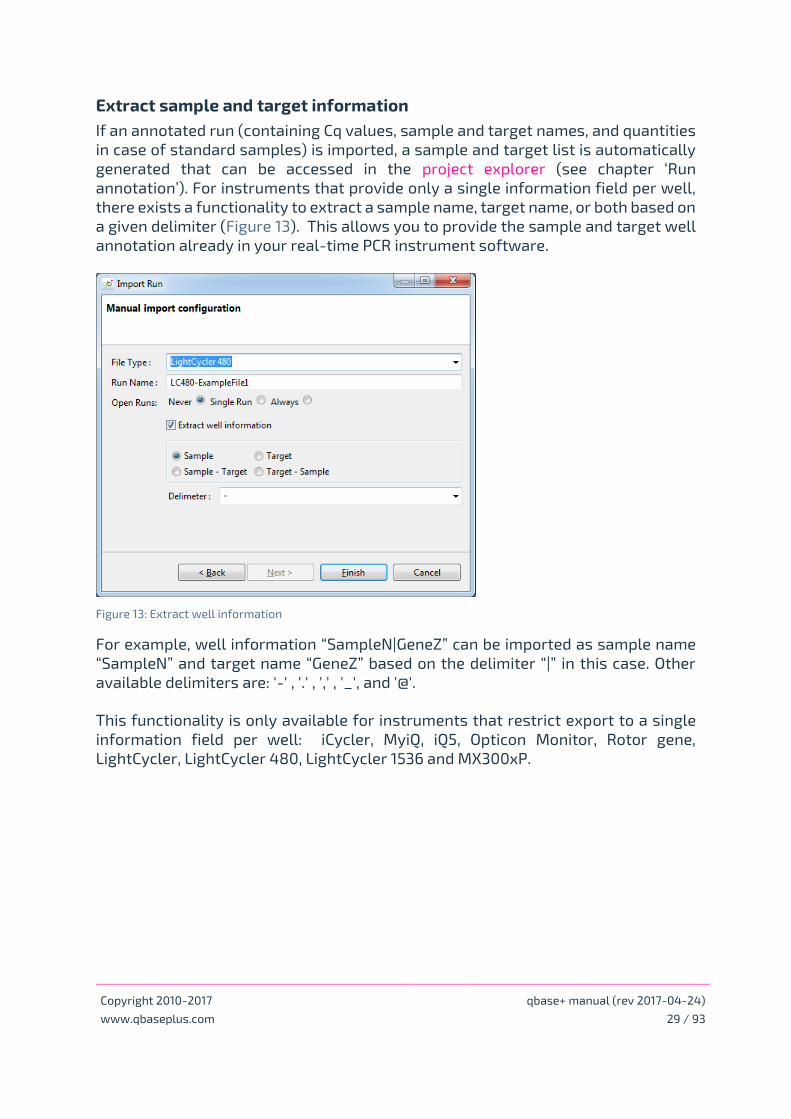
Extract sample and target information
If an annotated run (containing Cq values, sample and target names, and quantities
in case of standard samples) is imported, a sample and target list is automatically
generated that can be accessed in the project explorer (see chapter ‘Run
annotation’). For instruments that provide only a single information field per well,
there exists a functionality to extract a sample name, target name, or both based on
a given delimiter (Figure 13). This allows you to provide the sample and target well
annotation already in your real-time PCR instrument software.
Figure 13: Extract well information
For example, well information “SampleN|GeneZ” can be imported as sample name
“SampleN” and target name “GeneZ” based on the delimiter “|” in this case. Other
available delimiters are: '-' , '.' , ',' , '_', and '@'.
This functionality is only available for instruments that restrict export to a single
information field per well: iCycler, MyiQ, iQ5, Opticon Monitor, Rotor gene,
LightCycler, LightCycler 480, LightCycler 1536 and MX300xP.
Copyright 2010-2017 qbase+ manual (rev 2017-04-24)
www.qbaseplus.com 30 / 93
Complete run import
Click 'import' to complete the import run wizard. You will see that the runs are
added to your experiment and that they are automatically processed (unless you
disabled automatic recalculation in the Preferences window, see higher).
An individual window can be opened for each imported run by double clicking the
run in the project explorer tree. This allows editing of sample and target information
for each well. In addition, the sample and target list in the project explorer tree is
automatically updated with the sample and target names provided they are
included in the import files.
More information on the annotation of runs with target and sample names, sample
types and quantities for the standard samples can be found in chapter ‘Run
annotation’.
Samples and targets
qbase+ provides all the functionality for full annotation of wells (see ‘Run
annotation’ chapter). Samples and targets are created as part of the import of an
annotated run, or should be manually created in qbase+ (in case an unannotated run
was imported). Since users typically already have lists of samples and targets, it
may be more convenient to import those lists rather than to enter the information
in qbase+. This is especially true if the information not only lists sample names, but
also a series of sample property attributes (e.g. group to which a sample belongs).
The format of sample and target import files, as well as example files can be found
on the qbase+ website. The import procedure for both is very similar. We here
describe the procedure for the import of sample lists.
Start Import samples wizard
Right-click in the project explorer on samples (or any sample in the experiment
project explorer) to start the import samples wizard. The import button ( ) in the
toolbar will also lead to this wizard if selecting samples.
Select sample list
Select the experiment in which the sample list needs to be imported. By default, the
experiment selected in the project explorer is indicated as the target experiment.
Browse for your sample list file and click the next button.
Copyright 2010-2017 qbase+ manual (rev 2017-04-24)
www.qbaseplus.com 31 / 93
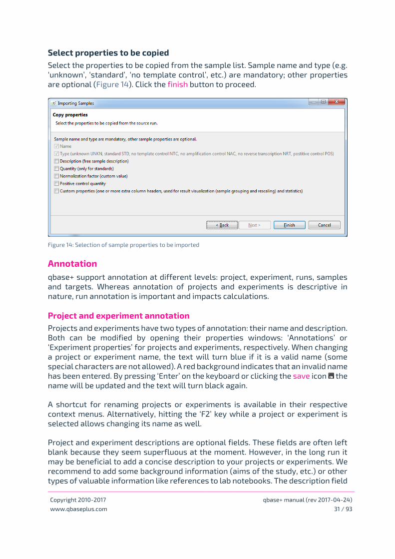
Select properties to be copied
Select the properties to be copied from the sample list. Sample name and type (e.g.
‘unknown’, ‘standard’, ‘no template control’, etc.) are mandatory; other properties
are optional (Figure 14). Click the finish button to proceed.
Figure 14: Selection of sample properties to be imported
Annotation
qbase+ support annotation at different levels: project, experiment, runs, samples
and targets. Whereas annotation of projects and experiments is descriptive in
nature, run annotation is important and impacts calculations.
Project and experiment annotation
Projects and experiments have two types of annotation: their name and description.
Both can be modified by opening their properties windows: ‘Annotations’ or
‘Experiment properties’ for projects and experiments, respectively. When changing
a project or experiment name, the text will turn blue if it is a valid name (some
special characters are not allowed). A red background indicates that an invalid name
has been entered. By pressing ‘Enter’ on the keyboard or clicking the save icon the
name will be updated and the text will turn black again.
A shortcut for renaming projects or experiments is available in their respective
context menus. Alternatively, hitting the ‘F2’ key while a project or experiment is
selected allows changing its name as well.
Project and experiment descriptions are optional fields. These fields are often left
blank because they seem superfluous at the moment. However, in the long run it
may be beneficial to add a concise description to your projects or experiments. We
recommend to add some background information (aims of the study, etc.) or other
types of valuable information like references to lab notebooks. The description field
Copyright 2010-2017 qbase+ manual (rev 2017-04-24)
www.qbaseplus.com 32 / 93
can hold multiple lines of information. Therefore the ‘Enter’ keyboard button cannot
be used to save the information. Use the save icon to save changes to the
description field (blue text will turn black).
Run annotation
Runs need to be properly annotated before experiments can be analyzed. Not only
will your data be meaningless without annotation, it is simply essential for qbase+
to start any calculations.
Runs can be annotated before or after import in qbase+. If an annotated run (i.e
containing a sample and target name for every well that has a Cq value) is imported,
qbase+ will take over this annotation and generate a sample and a target list. All
annotation can still be edited afterwards. In contrast, editing of Cq values is
explicitly not supported by qbase+, although one can choose to exclude certain data
points from calculations. Runs that were not annotated before import should be
annotated in qbase+, more specifically in the run editor.
The qbase+ run editor does not support well annotation by typing in sample or
target names. Sample and target names need to be selected from a dropdown list
at the top to annotate wells. This approach avoids spelling mistakes that are often
hard to spot and may undetectably lead to erroneous results.
Open run
Open a run by double-clicking its name in the project explorer, or use the open
option in the run context menu. The Run window contains a properties tab at the
bottom in which you can change the run name or alter the date on which the run was
generated. It also contains information regarding the format of the run. Samples
and targets can be appointed to wells in the matrix tab that depicts the run layout
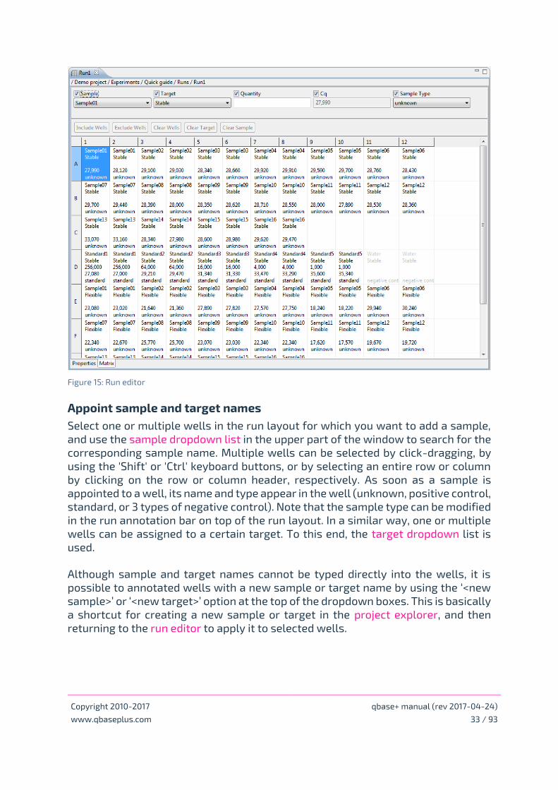
with an annotation bar on top (Figure 15).
Copyright 2010-2017 qbase+ manual (rev 2017-04-24)
www.qbaseplus.com 33 / 93
Figure 15: Run editor
Appoint sample and target names
Select one or multiple wells in the run layout for which you want to add a sample,
and use the sample dropdown list in the upper part of the window to search for the
corresponding sample name. Multiple wells can be selected by click-dragging, by
using the 'Shift' or 'Ctrl' keyboard buttons, or by selecting an entire row or column
by clicking on the row or column header, respectively. As soon as a sample is
appointed to a well, its name and type appear in the well (unknown, positive control,
standard, or 3 types of negative control). Note that the sample type can be modified
in the run annotation bar on top of the run layout. In a similar way, one or multiple
wells can be assigned to a certain target. To this end, the target dropdown list is
used.
Although sample and target names cannot be typed directly into the wells, it is
possible to annotated wells with a new sample or target name by using the ‘<new
sample>’ or ‘<new target>’ option at the top of the dropdown boxes. This is basically
a shortcut for creating a new sample or target in the project explorer, and then
returning to the run editor to apply it to selected wells.
Copyright 2010-2017 qbase+ manual (rev 2017-04-24)
www.qbaseplus.com 34 / 93
Quantities
For 'standard' (curve samples), an input quantity must be defined in the
corresponding field in the run annotation bar. In contrast to sample and target
information, quantities are not selected from a dropdown list but entered as a
numerical value. Note that quantity values cannot be added to sample types other
than ‘standard’. Also, since quantities are a sample property, changing the quantity
value for a standard sample in one well will alter the quantity value for that sample
in all wells in which it occurs. A sample quantity can also be entered by double-
clicking on the name of a ‘standard’ (curve) sample in the project explorer.
Exclusion
In the run layout window, you can select the wells that should to be excluded from
analysis. This option does not erase the Cq value nor the sample/target annotation,
meaning that excluded wells can later be re-included in the analysis if needed.
Note that empty wells and wells without Cq value are automatically excluded by
qbase+ and cannot be included by the user.
Clear
The options clear sample and clear target can be used to remove sample and target
names, respectively, from selected wells. It does not remove any other well
information. The clear wells option removes both the sample and target annotation.
The ‘undo’ and ‘redo’ options, available in the command bar, can be used to restore
accidentally removed annotation.
Apply/copy run layouts
To speed up run annotation, qbase+ enables copying the layout of samples, targets
or both from one run to another. When for instance the same set of samples is
measured in two different runs using the same layout (this is, the samples are
measured in the same position in both runs), sample annotation of a run only needs
to be performed once, saving you valuable time. This functionality can also be used
across different (open) experiments.
Start the ‘Apply run layout wizard’ by clicking the corresponding option in the
context menu of the run (or selection of multiple runs) for which you want to edit
the run information. Then, select the run that serves as a template. Note that only
runs can be selected from open (loaded) experiments. If needed, cancel the current
procedure and right-click on closed (unloaded) experiment and select load
experiment. Finally, select the properties that need to be copied (Figure 16). If
annotation information is already present in the destination run, a warning will be
displayed to notify you that information will be overwritten.

Copyright 2010-2017 qbase+ manual (rev 2017-04-24)
www.qbaseplus.com 35 / 93
Figure 16: Selection of information to be copied between runs
Sample annotation
There are three ways by which sample information can be provided to qbase+: as
part of the import of a run, by importing a sample list or by manually adding a
sample.
Creating new samples
There are four ways to create new samples:
1. by making use of the right-click context menu in the project explorer (right
click on the samples node and select new sample
2. by starting the new wizard by clicking on the command bar
3. by using the menu bar (File > New)
4. available in the run window only: select <new sample> from the sample drop
down box
In case of option 2 and 3: choose sample and subsequently select the experiment to
which the sample belongs. Click finish to complete the new wizard. Note that
samples can only be added to loaded (open) experiments. Experiments that are not
loaded are available for selection, but no sample can be added.

Copyright 2010-2017 qbase+ manual (rev 2017-04-24)
www.qbaseplus.com 36 / 93
Sample properties
Upon creation of a new sample, the sample window opens (Figure 17). This window
can also be accessed later by double-clicking the sample of interest. It allows for
reviewing and editing of sample annotation, including the sample name and type
(unknown sample, negative control, positive control, or standard), a custom
normalization factor and options for visibility in charts.
Figure 17: Sample type and information
When editing the sample description, blue text indicates unsaved entries.
Modifications can be saved by clicking the disc , or by closing the sample window.
In the latter case, a Save resource window opens that allows to save the
modifications. A red background indicates that illegal characters have been used
(see higher for overview of accepted characters).
Quantity values are linked to samples of type ‘standard’. Since one sample can only
have one quantity, the different dilutions of a given template should be given
different sample names (e.g. std1, std2, …), each with their quantity. If the import
contains different quantities for a single standard (curve) sample, qbase+ will only
retain the last value that is imported. You will need to manually edit sample names
and quantities.
Copyright 2010-2017 qbase+ manual (rev 2017-04-24)
www.qbaseplus.com 37 / 93
The custom normalization factor option allows the provision of a sample specific
custom normalization factor. This option enables normalization based on a user
provided value such as cell number count or mass/volume of the sample. Such
normalization can only be performed if a custom normalization factor is entered (or
imported) for all samples of interest.
The sample visibility in charts option allows indicating whether a specific sample or
sample type has to be shown in charts. By default, negative controls and standard
curve samples will not be shown. This results in more intuitive charts and gives
more control on the content and look of your results.
Preferences can be modified in top menu (Window > Preferences). By default, only
unknown samples and positive control samples are shown in the bar chart. Sample
specific settings overrule the preferences.
Custom sample properties
In addition to the generic sample properties that have been described above, qbase+
also supports custom properties. These allow the annotation of samples with
information that may vary between users and from one experiment to another.
Examples include treatment, passage number, cell type, etc. Custom sample
properties are always composed of a property and a property value, with properties
being common across all samples and property values that may vary between
samples. For example: treatment - control, treatment - low concentration,
treatment - high concentration, or cell type - chondrocyte, cell type - osteoblast.
Custom sample properties are useful to:
• group results in the bar charts
• rescale results to a group (e.g. control samples)
• perform statistical analyses by comparing grouped samples (i.e. samples
that have the same custom sample property)
Custom sample properties can be entered manually or imported as part of a sample
list. To add or edit custom sample properties, open the sample properties window
that is located in the annotations section. This window contains a list of samples
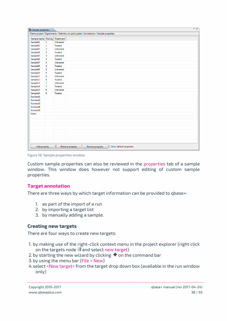
that may or may not have custom samples attached to them (Figure 18). Use the
buttons at the bottom of the window to add, remove or rename custom properties.
On creation of a new custom property, an extra column is added to the table. Sample
specific property values can be entered in this column.
Copyright 2010-2017 qbase+ manual (rev 2017-04-24)
www.qbaseplus.com 38 / 93
Figure 18: Sample properties window
Custom sample properties can also be reviewed in the properties tab of a sample
window. This window does however not support editing of custom sample
properties.
Target annotation
There are three ways by which target information can be provided to qbase+:
1. as part of the import of a run
2. by importing a target list
3. by manually adding a sample.
Creating new targets
There are four ways to create new targets:
1. by making use of the right-click context menu in the project explorer (right click
on the targets node and select new target)
2. by starting the new wizard by clicking on the command bar
3. by using the menu bar (File > New)
4. select <New target> from the target drop down box (available in the run window
only)

Copyright 2010-2017 qbase+ manual (rev 2017-04-24)
www.qbaseplus.com 39 / 93
In case of option 2 and 3: choose target and subsequently select the experiment to
which the target needs to be added (Figure 19). Click finish to complete the new
wizard. Note that targets can only be added to loaded (open) experiments.
Experiments that are not loaded are available for selection, but no targets can be
added.
Figure 19: Create new target in experiment ...
Target properties
On creation of a new target, the target window opens. This window can also be
accessed later by double clicking the target of interest. When creating a new target,
the target window opens in the properties tab. For existing targets, the target
window opens in the Bar chart. For reviewing and editing of target annotations one
needs to activate the properties tab.
There are two types of target information that are essential to qbase+: the target
name and the target type. The remaining information fields are there for annotation
purposes only.
Target type
Two types of targets are used in qbase+, targets of interest and reference targets.
Reference targets (also referred to as housekeeping genes, a name deprecated by
the MIQE guidelines, Bustin et al., 2009) are used for normalization. The target type
can be defined via the target properties window (see above), or by using the set
target type option from the context menu of selected targets in the project explorer
window. Multiple targets can be simultaneously appointed as reference targets or

Copyright 2010-2017 qbase+ manual (rev 2017-04-24)
www.qbaseplus.com 40 / 93
as targets of interest by selecting all of them using the 'Shift' or the 'Ctrl' (Windows)
or ‘Command’ (MacOSX) keyboard buttons.
Note that all targets labeled as reference targets are used in the multiple reference
gene normalization procedure (Vandesompele et al., 2002). To exclude one or more
reference targets, change their type into target of interest, which causes the
software to treat them as if they were targets of interest.
Renaming and clean-up
Existing sample or target names can be modified (rename) by double clicking their
name in the project explorer. A window opens where you can change the name (and
other properties). Alternatively, a name can be modified using the menu bar (Edit >
Rename), via the context menu or by using the ‘F2’ keyboard button (Figure 20).
Figure 20: Sample renaming
It is not possible to rename a sample or target to a name that is already in use. If a
given sample (or target) exists with two different names (e.g. due to typing error),
the replace option in the sample (target context menu should be used to replace the
incorrect sample (target) name with the correct one (to be selected from a drop
down list containing existing names).
Samples and targets can be deleted via their context menu (cursor needs to be on
the sample or target that should be deleted) or by selecting and clicking the delete
icon in the command bar. Multiple samples or targets can be simultaneously
deleted by selecting all of them.
Some run import types provide default sample/target names for all wells if
annotation has not been performed in the qPCR instrument software. This may lead
to long lists of samples/targets that clutter the experiment and impede proper run
annotation. qbase+ contains a clean-up function that removes all unused samples
or targets. It is typically applied after having cleared all incorrect run annotations.
The clean-up function can be found as an option in the context menu of samples and
targets, but not in the context menus of individual samples or targets.
Copyright 2010-2017 qbase+ manual (rev 2017-04-24)
www.qbaseplus.com 41 / 93
Calculation parameters and quality control settings
The calculation parameters and quality control settings windows can be opened by
double clicking their respective icons under the settings node of your experiment in
the project explorer tree. Similar settings can be found at the level of a project.
These default experiment settings will not affect any existing experiment within
that project, but will be used as the default values when creating new experiments.
Calculation parameters
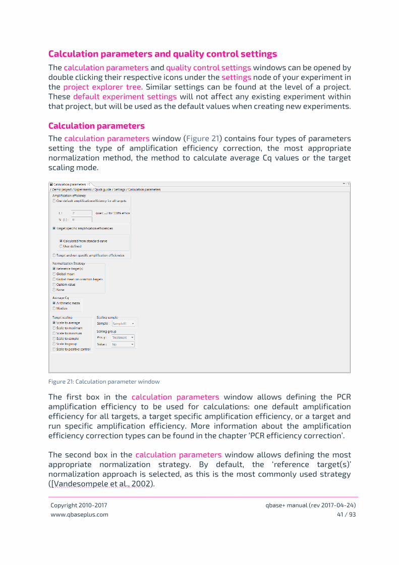
The calculation parameters window (Figure 21) contains four types of parameters
setting the type of amplification efficiency correction, the most appropriate
normalization method, the method to calculate average Cq values or the target
scaling mode.
Figure 21: Calculation parameter window
The first box in the calculation parameters window allows defining the PCR
amplification efficiency to be used for calculations: one default amplification
efficiency for all targets, a target specific amplification efficiency, or a target and
run specific amplification efficiency. More information about the amplification
efficiency correction types can be found in the chapter ‘PCR efficiency correction’.
The second box in the calculation parameters window allows defining the most
appropriate normalization strategy. By default, the ‘reference target(s)’
normalization approach is selected, as this is the most commonly used strategy
([Vandesompele et al., 2002).

Copyright 2010-2017 qbase+ manual (rev 2017-04-24)
www.qbaseplus.com 42 / 93
In addition to normalization using one or multiple reference genes, qbase+ supports
a range of different normalization procedures to suit the specific needs of different
types of experiments.
Reference targets
This is qbase+’s default normalization procedure. Depending on the number of
selected reference targets, relative quantities will be normalized by the relative
quantity of a single reference target or by the geometric mean of the relative
quantities for all reference targets.
Global mean - premium license only
The global mean normalization procedure was initially developed for the
normalization of extended miRNA screening experiments where it was shown
to be a superior alternative to the commonly used small nuclear and small
nucleolar RNAs as reference targets (Mestdagh et al., Genome Biology, 2009). It
is however useful for any experiment in which a sufficiently large set of
unbiased genes is quantified. It is based on the same principles commonly used
for microarray normalization. The results for a given sample will be normalized
by the geometric mean of the relative quantities of all the targets that are
expressed in that sample. The global mean normalization method in qbase+ is
an improved version of the Mestdagh et al. method by giving equal weight to
each target [D’haene et al., Methods in Molecular Biology, 20112].
Global mean on common targets - premium license only
Similar to the ‘Global mean’ normalization procedure with the exception that the
normalization factor will only be based on the targets that are expressed in all
samples.
Custom value
This option enables normalization based on a user provided value such as cell
number. In this method, a custom normalization factor should be provided for
every sample, or be imported as a sample property.
None
This option is included to enable qPCR data-analysis for which normalization
may not be appropriate, e.g. absolute quantification or single cell analysis.
The third box in the calculation parameters window allows defining the method by
which average Cq values are calculated. In addition to the (default) arithmetic mean
on replicated Cq value measurements, qbase+ also supports the calculation of
median Cq values. The median Cq value is a more robust measure than the
arithmetic mean when confronted with outliers and having at least 3 PCR replicates.
Median results (without outlier removal) are a good alternative to arithmetic
averages calculated on datasets in which outliers have been removed.
Copyright 2010-2017 qbase+ manual (rev 2017-04-24)
www.qbaseplus.com 43 / 93
The fourth box in the calculation parameters window allows setting the scaling of
the normalized relative quantities (NRQ values) and the corresponding target bar
charts. Please note, that target scaling will not affect the result of the analysis. By
default, the results are scaled to the average across all unknown samples per
target, which means that the average across all unknown samples is set to one.
Similarly, when selecting the option scale to maximum, scale to minimum, or scale
to sample the maximum, minimum, or a particular sample are set to 1. scale to group
is only possible after having defined sample groups in the Sample properties
window. scale to positive control is useful for copy number analysis and allows you
to indicate the copy number in your calibrator samples (see chapter ‘Copy number
analysis’).
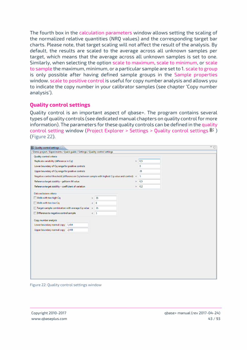
Quality control settings
Quality control is an important aspect of qbase+. The program contains several
types of quality controls (see dedicated manual chapters on quality control for more
information). The parameters for these quality controls can be defined in the quality
control setting window (Project Explorer > Settings > Quality control settings )
(Figure 22).
Figure 22: Quality control settings window

Copyright 2010-2017 qbase+ manual (rev 2017-04-24)
www.qbaseplus.com 44 / 93
The first box in the quality control settings window contains parameters that do not
affect calculations, but merely set the thresholds beyond which data are flagged for
low quality. The quality control parameters include a threshold for maximum
replicate variability, a range of acceptable Cq values for positive controls, a delta-
Cq value for the interpretation of negative controls, and two thresholds for
assessment of reference target stability.
In the second box in the quality control settings window contains criteria for
automatic exclusion of certain data points. These settings do impact the final
experiment results. The ‘Difference to negative control sample < …’ is used to
automatically exclude data points that could be significantly impacted by the signal
found in the negative control. The ‘Well with too high Cq > …’ and ‘Well with too low
Cq > …’ are used to automatically exclude data points in a Cq range with inaccurate
results. Similarly, the ‘Target-sample combination with average Cq value > …’ can
be used to automatically exclude replicates with an average Cq in the range with
inaccurate results. The latter two options are particularly relevant when analyzing
whole genome miRNA expression profiles with the new global mean normalization
approach.
Data points that have been automatically excluded are grayed out in the replicate
quality control. These data points, like those that have been manually excluded, will
not be used for calculations. In contrast to manually excluded data points they
cannot be re-included in the replicate quality control screen or the run editor, i.e.
they are strictly linked to the auto exclusion settings.
Specific for qPCR-based copy number analysis (premium license only) is the
definition of the thresholds for the lower boundary for normal copy and the upper
boundary for normal copy in the third box. These thresholds are used for conditional
bar coloring for easy detection of deletions and amplifications and are by default
set to 1.414 (geometric mean of 1 and 2 copies) and 2.449 (geometric mean of 2 and
3). These default settings are recommended for a diploid organism (like human,
mouse and rat), and may need to be adjusted for polyploid organisms.

Copyright 2010-2017 qbase+ manual (rev 2017-04-24)
www.qbaseplus.com 45 / 93
Inter-run calibration
Inter-run calibration is a calculation procedure to detect and remove (often
underestimated) inter-run variation. Whenever samples need to be compared that
are measured in different runs, one should be cautious of this potential bias.
Importantly, inter-run calibration is needed for each gene separately. Detailed
information is available in the original qBase paper (Hellemans et al., Genome
Biology, 2007).
The basic principle is that the experimenter measures one or (preferentially) more
identical samples in different (to be calibrated) runs, in addition to the other
samples that are spread across the runs. The results for these identical samples
(so-called inter-run calibrator or IRC samples) can then be used to quantify and
correct inter-run variation. By measuring the difference in Cq or normalized relative
quantity between the IRCs in the different runs, it is possible to calculate a
correction or calibration factor to remove the run-to-run difference, and proceed as
if all samples were measured in the same run.
The inter-run calibration concept
In a relative quantification study, the experimenter is usually interested in
comparing the expression level of a particular gene between different samples.
Reliable estimates for relative expression levels can only be obtained by minimizing
and correcting technical variations between samples and measurements. It is well
recognized that variations in the target nucleic acids input amount between
samples need to be corrected by means of normalization, typically using one or
multiple reference genes. Run-to-run variation within a series of measurements for
a given gene is a second type of technical variation that needs to be avoided,
minimized or corrected for.
We advise to follow the sample maximization method (Figure 23), which dictates
that all samples (or as many as possible) for a given gene should be analyzed in the
same run. The sample maximization strategy does not suffer from technical (run-
to-run) variation between samples, and therefore does not require inter-run
calibration to be performed. Since reference genes, independently of the other
assays, quantify the relative concentration of nucleic acids between samples there
is no need to repeat the measurement of the reference genes in every run.
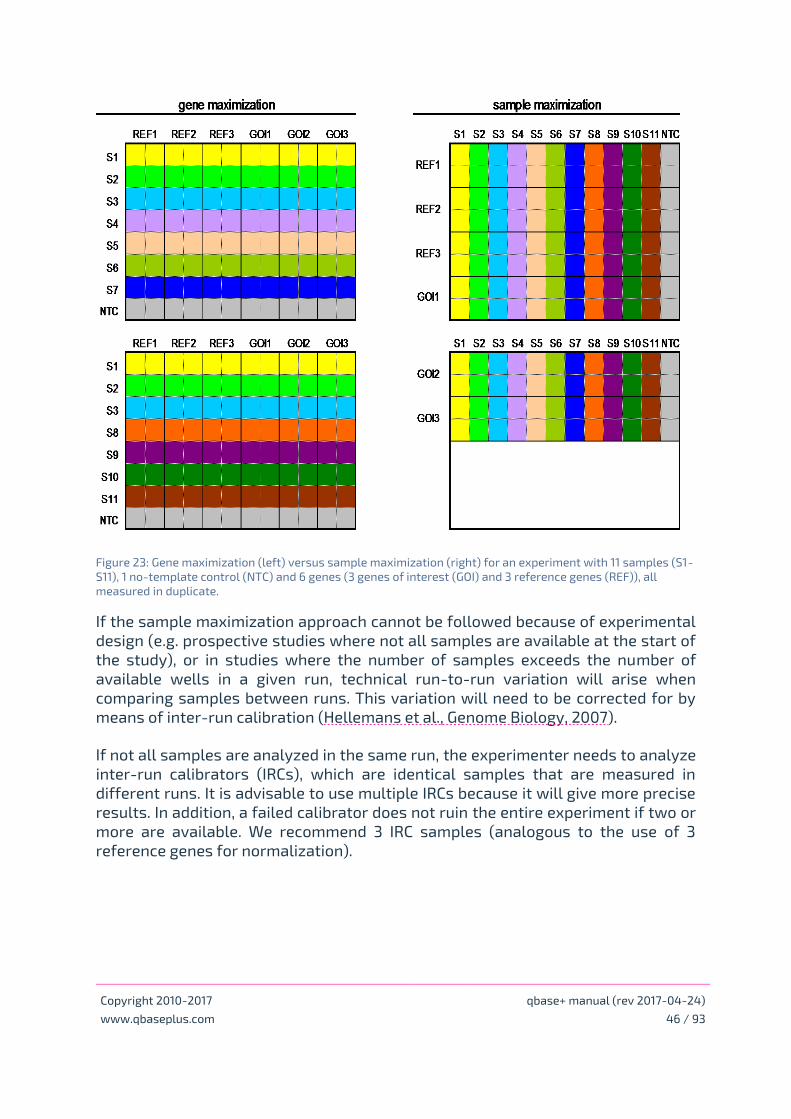
Copyright 2010-2017 qbase+ manual (rev 2017-04-24)
www.qbaseplus.com 46 / 93
Figure 23: Gene maximization (left) versus sample maximization (right) for an experiment with 11 samples (S1-
S11), 1 no-template control (NTC) and 6 genes (3 genes of interest (GOI) and 3 reference genes (REF)), all
measured in duplicate.
If the sample maximization approach cannot be followed because of experimental
design (e.g. prospective studies where not all samples are available at the start of
the study), or in studies where the number of samples exceeds the number of
available wells in a given run, technical run-to-run variation will arise when
comparing samples between runs. This variation will need to be corrected for by
means of inter-run calibration (Hellemans et al., Genome Biology, 2007).
If not all samples are analyzed in the same run, the experimenter needs to analyze
inter-run calibrators (IRCs), which are identical samples that are measured in
different runs. It is advisable to use multiple IRCs because it will give more precise
results. In addition, a failed calibrator does not ruin the entire experiment if two or
more are available. We recommend 3 IRC samples (analogous to the use of 3
reference genes for normalization).

Copyright 2010-2017 qbase+ manual (rev 2017-04-24)
www.qbaseplus.com 47 / 93
Different types of input material can be used to create IRC samples: real samples
for which sufficient material is available to measure them in different runs; pools of
samples; synthetic templates (e.g. external oligonucleotide standards, see
Vermeulen et al., Nucleic Acids Research, 2009); etc. Serial dilutions (standard
curve) often make good IRC samples (make sure to give each dilution a different
sample name in qbase+).
Importantly, inter-run calibration should be performed on a gene per gene basis. It
is not sufficient to quantify the inter-run variation for a single assay and to
extrapolate this result to other assays. The experimenter should perform inter-run
calibration for all genes/assays.
Inter-run calibration in qbase+
qbase+ performs inter-run calibration after data normalization. This does not only
result in fewer calculations, but provides more flexibility as a new batch of cDNA
can be synthesized from the inter-run calibrator RNA samples while still remaining
a valid inter-run calibrator. It does however put some limitations on the design of
the study.
When designing a qPCR experiment and determining how measurements will be
spread across runs, different approaches can be chosen: 1) all samples for a given
gene within a single run, 2) all genes for a given sample within a single run, 3) both
samples and genes are spread across runs. The first approach does not require
inter-run calibration, the second approach is 100% compatible with the inter-run
calibration that is being performed by qbase+. Inter-run calibration for the third
approach is only valid when specific requirements are met: the same set of inter-
run calibrators is used in every run (and for every gene) and samples are grouped
into runs in the same way across the entire experiment.
qbase+ recognizes PCR replicates based on identical sample and target names. For
qbase+ not to interpret IRC data points as PCR replicates, the IRCs should have a
different sample name in each run. Assuming sampleA is used as inter-run
calibrator, it could be named sampleA_1 in the first run, sampleA_2 in the 2nd run,
etc. The same procedure should be used for all genes within your experiment (to
make sure normalization is performed correctly).
Some researchers deliberately split PCR replicates over 2 runs. Although this
approach is supported by qbase+, it is not compatible with inter-run calibration. If
inter-run variation is a concern that you want to correct for by means of inter-run
calibration, you should not introduce this type of variation by spreading replicates
across run.

Copyright 2010-2017 qbase+ manual (rev 2017-04-24)
www.qbaseplus.com 48 / 93
If samples are analyzed across multiple runs for a given target and if no IRC samples
have been appointed, the user will be notified by an alert message in the alerts
window (Figure 24) and by the appearance of the message 'IRC Missing' in the
calibration factors window.
Figure 24: Alert for potential inter run variation
Open the interrun calibration window
Open the interrun calibration window from the project explorer (intermediate
results > interrun calibration) by double clicking it, or by using the open option from
its context menu. Two tabs are available in this window: interrun calibrators and
calibration factors. The calibration factors tab is shown by default (Figure 25).
Because no IRC information is available, all calibration factors (CF) are set to 1.
Figure 25: Defining inter run calibrators
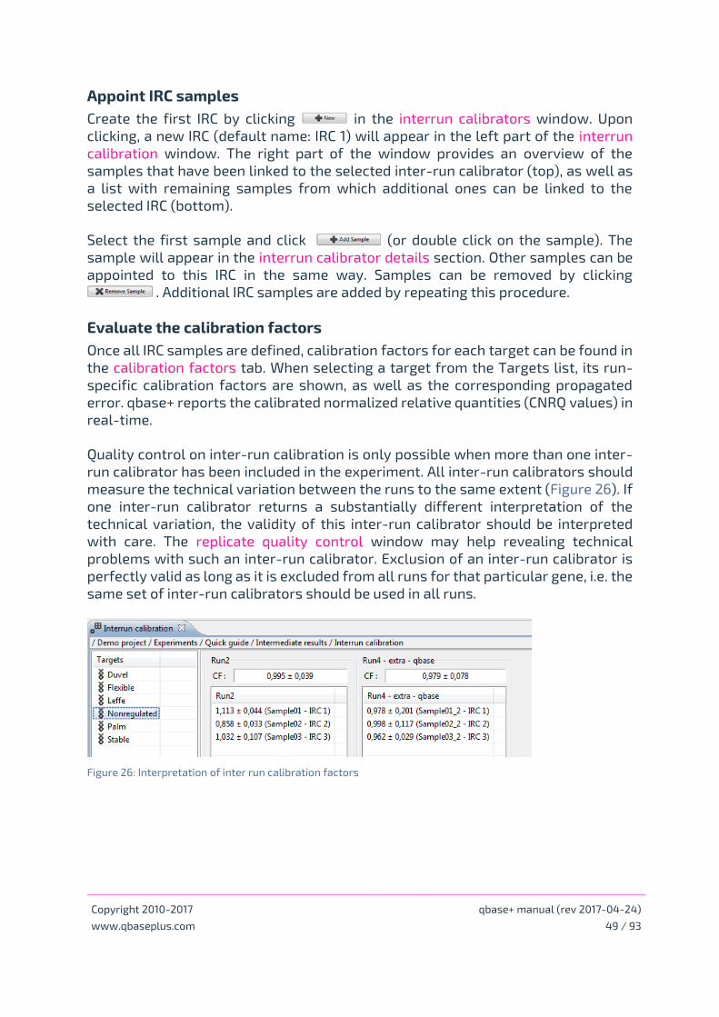
Copyright 2010-2017 qbase+ manual (rev 2017-04-24)
www.qbaseplus.com 49 / 93
Appoint IRC samples
Create the first IRC by clicking in the interrun calibrators window. Upon
clicking, a new IRC (default name: IRC 1) will appear in the left part of the interrun
calibration window. The right part of the window provides an overview of the
samples that have been linked to the selected inter-run calibrator (top), as well as
a list with remaining samples from which additional ones can be linked to the
selected IRC (bottom).
Select the first sample and click (or double click on the sample). The
sample will appear in the interrun calibrator details section. Other samples can be
appointed to this IRC in the same way. Samples can be removed by clicking
. Additional IRC samples are added by repeating this procedure.
Evaluate the calibration factors
Once all IRC samples are defined, calibration factors for each target can be found in
the calibration factors tab. When selecting a target from the Targets list, its run-
specific calibration factors are shown, as well as the corresponding propagated
error. qbase+ reports the calibrated normalized relative quantities (CNRQ values) in
real-time.
Quality control on inter-run calibration is only possible when more than one inter-
run calibrator has been included in the experiment. All inter-run calibrators should
measure the technical variation between the runs to the same extent (Figure 26). If
one inter-run calibrator returns a substantially different interpretation of the
technical variation, the validity of this inter-run calibrator should be interpreted
with care. The replicate quality control window may help revealing technical
problems with such an inter-run calibrator. Exclusion of an inter-run calibrator is
perfectly valid as long as it is excluded from all runs for that particular gene, i.e. the
same set of inter-run calibrators should be used in all runs.
Figure 26: Interpretation of inter run calibration factors
Copyright 2010-2017 qbase+ manual (rev 2017-04-24)
www.qbaseplus.com 50 / 93
Quality control and results
PCR efficiency correction
qbase+ employs a universal and flexible quantification model (Hellemans et al.,
Genome Biology, 2007). Depending on the selected option in the amplification
efficiency box of the calculation parameters window, this model will either equal
the delta-delta-Ct method described by Livak and Schmittgen or the efficiency
corrected model described by Pfaffl. The former assumes 100% amplification
efficiency for all targets, whereas the latter supports correction for target specific
amplification efficiencies.
There are several ways to approach PCR efficiencies. One could assume that all
assays perform perfectly. This is the most straightforward, but not the
recommended approach. We advise to assess the amplification efficiency for all
targets. The gold standard for efficiency correction is the use of standard curves.
This approach is supported by qbase+. Alternatively, any of the various algorithms
that have been described to estimate the PCR efficiency based on a single
amplification curve might be used. Unfortunately, many of these methods do not
provide a precise or an accurate estimate of the efficiency. One should therefore be
cautious in using these single reaction PCR efficiency values; it is generally
recommended to calculate the mean efficiency of all reaction wells in which the
same target is amplified (more information in Karlen et al., BMC Bioinformatics,
2007 – Jan Ruyter). Since qbase+ does not read raw fluorescence values, this latter
approach can not be supported.
qbase+ uses the base of the exponential function (E value) as the amplification
efficiency value for relative quantification (see formula 5 in Hellemans et al.,
Genome Biology, 2007). This base is the efficiency value + 1, e.g. an E value of 1.95
for 95% efficiency (efficiency value of 0.95).
Use one default amplification efficiency
When using the same amplification efficiency for all targets, either as an
assumption or because this has been proven before, one should select the ‘One
default amplification efficiency’ option in the calculation parameters window. The
actual value for E (efficiency + 1) can also be entered in this window. If known, the
error on the estimated efficiency could also be provided. Default values for E and
SE(E) are 2 and 0, respectively. These values correspond to what is assumed in the
delta-delta-Cq quantification model as originally described by Livak and Schmittgen
(Methods, 2001).

Copyright 2010-2017 qbase+ manual (rev 2017-04-24)
www.qbaseplus.com 51 / 93
Use target specific amplification efficiencies
The gold standard method for PCR efficiency estimation is a serial dilution of nucleic
acid template that is as similar to the samples under investigation as possible (e.g.
a mixture of cDNA from a representative set of your samples). We have observed
that the use of small synthetic templates (e.g. comprised of the first 30 and the last
30 bases of the amplicon sequence) is a cheap and easy alternative that results in
equivalent efficiency estimates.
qbase+ offers the possibility to make use of target specific amplification efficiencies
by selecting the ‘target specific amplification efficiencies’ option in the calculation
parameters window. This option may be used for experiments in which serial
dilutions or standard curves are included, or whenever these efficiency values have
been determined before.
The E value can be calculated from the slope of a serial dilution as follows: E = 10(-
1/slope) (with an E of 2 being perfect, indicating 100% efficiency). In our own
experiments, we aim for E values in the range of 1.90 – 2.10 (PCR efficiency between
90 and 110%) with standard errors typically below 0.01 (1%). The Y-intercept is only
meaningful when actual concentrations or template copy counts are used to define
the quantities for standard samples. It may be used to estimate the Cq value that is
expected for qPCR reactions with just a single molecule of template. Cq values
beyond this Y-intercept value may indicate primer dimer formation (for SYBR
reactions) or inhibited amplification. The Y-intercept may also provide valuable
information about the Cq range in which a considerable degree of sampling noise
may be expected; this is down to 3 or 4 cycles below the Y-intercept. It may also
yield additional insights in the performance of the assay. High Y-intercepts typically
coincide with low amplification efficiencies. If these occur for assays with good
efficiencies (90%-110%) they may indicate problems to generate the first PCR
copies, e.g. due to strong secondary structures in or around the primer binding sites.
The amplification efficiency window can be opened by double clicking ‘amplification
efficiency’ in the project explorer (Figure 27). Depending on the option chosen in the
calculation parameters window either the computed or user-defined is greyed out
(disabled). With ‘Target specific amplifciation efficiencies’ set to user-defined the
user has the opportunity to manually enter an efficiency value for each target by
providing a ‘user-defined’ E-value.

Copyright 2010-2017 qbase+ manual (rev 2017-04-24)
www.qbaseplus.com 52 / 93
Figure 27: Amplification efficiency window
By unticking the box in front of an outlier well, certain dilution points can be
excluded from the calculation of the efficiency value. By hovering over a data point
in the standard curve, the identity of an outlier reaction is easily determined.
Make amplification efficiencies run specific
If a target is measured in different runs, and a serial dilution for that target is
present in each run, qbase+ offers the possibility to use a run-specific target
amplification efficiency. Hence, each Cq value will be converted to a relative
quantity (RQ) using the efficiency measured in that particular run.
Quality controls
Quality control is an important feature in qbase+. The program contains several
types of quality control that can be accessed by double-clicking the quality control
icon in the project explorer:
• quality control on technical replicates
• quality control on positive and negative controls
• quality control on the stability of reference targets
• quality control on different sample specific characteristics
The parameters for quality control can be defined in the quality control setting
window (Project Explorer > Settings > Quality control settings ).
More information about post-PCR quality control can be found in the paper ‘The
Importance of Quality Control During qPCR Data Analysis’ (D’haene and Hellemans,
International Drug Discovery, 2010).

Copyright 2010-2017 qbase+ manual (rev 2017-04-24)
www.qbaseplus.com 53 / 93
Technical replicates
qbase+ automatically deals with technical replicates or repeated measurements,
which are recognized as different PCR wells with an identical sample and target
name. Importantly, we highly recommend measuring all PCR replicates in the same
run. If PCR replicates are measured in different runs, an alert will be displayed in the
alert window (‘PCR replicates (wells with identical sample and target name) are
spread across runs. This assumes that you have controlled for inter-run variation.’).
The Cq values of all (non-empty) wells of a replicate group are averaged at the very
beginning of the calculation process. Outliers can be excluded so they do not take
part in the calculations.
Inspecting replicate quality control
The replicates window (Project explorer > Quality control) contains an overview
of all replicate groups (defined by wells with the same target and sample name)
(Figure 28). The summary on top of the list contains the pass rate of the replicates
and informs the user about the overall replicate quality of the experiment.
Figure 28: Table of replicates failing to meet the set quality criteria
qbase+ can selectively display the failed replicates, i.e. replicates that do not meet
the quality threshold as defined in the quality control settings. This is done by
checking the ‘failing’ option in the well selection box. Other visualization options
include ‘all’ and ‘excluded’. The first option may be disabled for very large
experiments. The last option can be used to reinclude data points that have been
incorrectly excluded, or to inspect the wells that have been excluded by means of
auto exclusion.
In larger experiments it may be interesting to inspect the distribution of replicate
variability. A delta-Cq frequency histogram can be inspected in normal or in
cumulative mode by clicking on the corresponding tabs (frequency or cumulative)
at the bottom of the replicates window.

Copyright 2010-2017 qbase+ manual (rev 2017-04-24)
www.qbaseplus.com 54 / 93
Excluding bad replicates
Failing replicates can be excluded from further calculations by removing the tick in
front of the well (second column in the table). The number of failed replicates is
determined by the quality of the data in combination with the quality control
settings . qbase+ flags bad replicates based on a user defined maximum allowed
difference in Cq value. This value can be defined in the quality control settings
window in the replicate variability box. By default, the replicate variability threshold
is set to 0.5, which means that the difference in Cq value between the replicate with
the highest Cq value and the replicate with the lowest Cq value (∆Cq) must be
smaller than 0.5 cycles.
If a more stringent quality control is used (which is equal to a lower threshold
value), more replicates will fail the quality control: the list of failed replicates will
be longer and the summary will report a lower pass rate.
Individual PCR replicates should only be excluded if there is a good, objective reason
to do so (e.g. abnormal melt curve, no sample added). When in doubt, keep all
replicates, as the higher replicate variability will simply result in a larger propagated
error on the final result. With 3 or more PCR replicates one could look for statistical
outliers among the PCR replicates. Alternatively, one could simply opt to use the
median Cq instead of the arithmetic mean of Cq values in the calculation parameters
window. This approach results in a more robust measure for the average Cq without
the need for meticulous inspection and correction of all replicates failing the quality
control.
PCR replicates (repeated measurements of the same sample in the same run) are
useful for a number of reasons:
• it allows for quality control on the technical reproducibility of the qPCR data
• provides better accuracy
• allows the generation of results when individual qPCR reactions failed
Strict guidelines on the optimal number of PCR replicates cannot be given since it
depends on the purpose of the study (e.g. diagnostics versus research), the quality
of the PCR assay, the precision of the qPCR instrument, the Cq determination
method, and the pipetting skills of the operator. Ultimately, it all comes down to
determine how much confidence is needed for a given data point.
Important to note is that the biological variability is often much larger than the
technical variability. Therefore, it is acceptable to omit PCR replicates when the
sample size is sufficiently large or when a screening experiment is run (as is often
the case for miRNA expression profiling studies).

Copyright 2010-2017 qbase+ manual (rev 2017-04-24)
www.qbaseplus.com 55 / 93
By placing the quality control settings window next to the replicates window, you
can see the effect of changing the replicate variability threshold in real-time. More
information on the flexible use of windows in qbase+ is available in the ‘User
interface’ chapter.
Positive and negative controls
The second type of quality control is evaluation of the positive and negative sample
controls. The +/- controls window (Project explorer > Quality Control) shows a
summary of the QC results and a list of the samples that can be filtered for those
that faile the quality control (Figure 29). qbase+ flags suspicious no-template
control (NTC) samples based on a user defined threshold that can be found in the
quality control settings window . The default value is flagging of non-negative
NTC results that are less than 5 cycles away from the sample of interest with the
highest Cq value. For positive controls, a range of acceptable Cq values can be set in
the quality control settings window. The default range includes any meaningful Cq
value, i.e. Cq between 5 and 35.
Figure 29: List of data for all negative controls in the +/- controls window
In order to get a result for the positive and negative controls, positive and negative
control samples should be appropriately labeled in the sample list. If not, no results
are shown in the +/- controls window. More information on the annotation of
samples can be found in the ‘Annotation’ chapter.
An amplification signal in the NTC sample indicates a potential contamination issue
or formation of primer dimers. Such problems can be ignored as long as the
difference in Cq value between the NTC and the sample with the highest Cq value is
sufficiently large. For example, a Cq value difference of 5 corresponds to a fold
difference of about 32, indicating that approximately 3 % of the signal in your
samples may be caused by these unwanted signals (well below the technical error
on PCR replicates). Smaller differences between the NTC and the unknown samples
should be avoided.

Copyright 2010-2017 qbase+ manual (rev 2017-04-24)
www.qbaseplus.com 56 / 93
Stability of reference targets
When using the multiple reference target normalization approach (Project explorer
> Settings > Calculation parameters), reference target stability is the third type of
quality control. The user is able to choose a minimal acceptable reference target
stability by defining a threshold value for two indicators of expression stability of
the used reference genes: the geNorm expression stability value of the reference
gene (M) and the coefficient of variation of the normalized reference gene relative
quantities (CV) [Vandesompele et al., Genome Biology, 2002; Hellemans et al.,
Genome Biology, 2007]. Both parameters are automatically calculated by qbase+
during the analysis. More information on finding the best set of reference genes in
a given experimental condition can be found in the ‘geNorm’ chapter.
In order to get a result for the reference target stability, at least two reference
targets have to be appointed. No quality control results will be shown in the
reference target stability window (Figure 30 – top) if no reference targets or just a
single one have been appointed. The algorithm used to evaluate the reference
target stability does require all samples to have results for all their reference
targets. In case of missing data, no stability measures can be calculated and NaN is
shown in the reference target stability window. Either deleting those sample(s) or
making the reference target with missing data a target of interest.
The threshold value for M and CV can be set in the quality control settings window
(Figure 30 – bottom). By default, these thresholds are set to 0.5 for the M value and
0.2 for the CV value. M and CV values passing the QC are highlighted in green in the
reference target stability window while failing ones are highlighted in red.
Figure 30: Quality control on reference target stability

Copyright 2010-2017 qbase+ manual (rev 2017-04-24)
www.qbaseplus.com 57 / 93
Sample quality control
The sample quality control window covers three ways to evaluate whether certain
samples fall outside the expected range in terms of their normalization factor, the
fraction of detected targets or the average Cq value. The tabs at the bottom of this
window can be used to switch between the different options to quality control
samples.
Normalization factors
Inspection of normalization factors allows you to inspect possible experimental
problems. Using approximately equal amounts of equal quality input material and
stably expressed reference genes, the normalization factor values should be similar
for all samples. Evaluation of normalization factors may reveal samples for which
less than the expected quantity of DNA was detected by the reference target assays.
Possible explanations include:
• a known shortage of template DNA
• an unexpectedly low cDNA quantity resulting from RNA degradation or failed
reverse transcription
• the presence of inhibitors leading to impaired PCR amplification
• differential expression of reference targets in this sample resulting in an
unreliable normalization
A variation of 2- to 3-fold is generally acceptable (this is the experimental variation
that you want to remove in the normalization process). Any higher variation should
be treated with care (Figure 31).
Figure 31: Quality control on sample normalization with a potential issue in sample 13
Copyright 2010-2017 qbase+ manual (rev 2017-04-24)
www.qbaseplus.com 58 / 93
The results of this quality control window are identical to those in the normalization
factors window as part of the intermediate results in the project explorer. In
addition to the graphical representation used for sample quality control, that
window can also visualize results in tabular format. Use the tabs at the bottom to
switch graphical and tabular format. This table can be exported by using the export
normalization factors option in the normalization factor context menu, or by using
the export wizard launched by clicking the upwards pointing arrow in the command
bar.
Detected targets
Assessment of the fraction of targets being detected per sample is typically applied
in screening experiments comparing the expression levels of larger numbers of
genes (including miRNAs). The results of this analysis may be used as an alternative
to the normalization factor analysis in experiments that have been normalized with
the global mean approach.
Mean Cq
Inspection of mean Cq values per sample is a third alternative for analysis of the
consequences of sample quantities. It may also be used to reveal challenges with
lowly expressed genes, having Cq values close to the detection limit.
Bar charts, correlation plots and results tables
qbase+ supports several ways to investigate qPCR experiment results. Most will use
target bar charts for the comparison of expression levels for a given gene between
different samples. In addition to this, qbase+ also supports the comparison of
expression profiles between different genes, either in a multi-target bar chart or in
a correlation plot. All results are also available in tabular format, most relevant for
further downstream processing.
Without altering the interpretation of the results, the actual values can still be
changed by selecting a different scaling option. By default, results are scaled to the
average for all the samples of a given target using the mathematics described in the
qBase paper. It may be more convenient to apply rescaling to a given sample or
sample group, often a reference sample or a group of normal controls.
Target bar charts
qbase+ has two ways to investigate qPCR results for a given target in bar charts.
Similar charts are obtained by double clicking a target in the project explorer or by
opening the target bar chart window located in the analysis section of the project
explorer (Figure 32). The charts and the options are identical between both
approaches. They do however differ in the fact that the first approach is specific for
the selected target, whereas the latter approach allows for easy switching between
different targets. One approach may be more convenient for the interpretation of

Copyright 2010-2017 qbase+ manual (rev 2017-04-24)
www.qbaseplus.com 59 / 93
just a single target or for the side-by-side comparison of two targets. The other
approach is better suited for the serial analysis of one target after the other.
Figure 32: Target bar chart
The target bar chart plots the relative quantities of one sample compared to the
others. The scale of these graphs is meaningless – the ratios between samples are
of importance. The error bars on the bars represent the standard errors of the
relative quantities. The size of these error bars has been calculated by propagating
all relevant errors: replicate variability, uncertainty on the estimated amplification
efficiency and the error on the normalization factors. The mathematics behind these
error calculations are described in the qBase paper. Because of the multiple sources
of errors it is possible that the results for a sample with just one replicate do have
error bars.
The bottom of Target bar chart window contains a few options to change the way
results are visualized. The Y-axis can be plot in linear or logarithmic scale. In view
of the nature of relative expression levels (expressed as fold changes) it makes
perfect sense to plot the result in log scale. On the other hand, many users may be
more familiar with the linear scale.
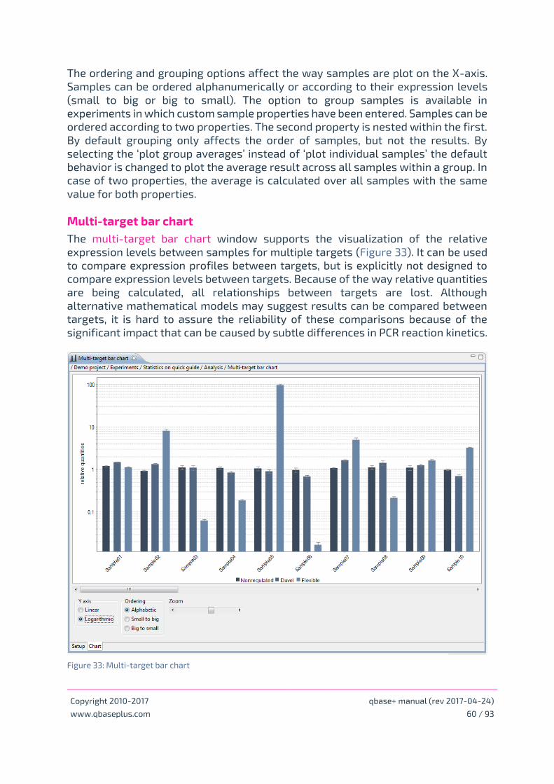
Copyright 2010-2017 qbase+ manual (rev 2017-04-24)
www.qbaseplus.com 60 / 93
The ordering and grouping options affect the way samples are plot on the X-axis.
Samples can be ordered alphanumerically or according to their expression levels
(small to big or big to small). The option to group samples is available in
experiments in which custom sample properties have been entered. Samples can be
ordered according to two properties. The second property is nested within the first.
By default grouping only affects the order of samples, but not the results. By
selecting the ‘plot group averages’ instead of ‘plot individual samples’ the default
behavior is changed to plot the average result across all samples within a group. In
case of two properties, the average is calculated over all samples with the same
value for both properties.
Multi-target bar chart
The multi-target bar chart window supports the visualization of the relative
expression levels between samples for multiple targets (Figure 33). It can be used
to compare expression profiles between targets, but is explicitly not designed to
compare expression levels between targets. Because of the way relative quantities
are being calculated, all relationships between targets are lost. Although
alternative mathematical models may suggest results can be compared between
targets, it is hard to assure the reliability of these comparisons because of the
significant impact that can be caused by subtle differences in PCR reaction kinetics.
Figure 33: Multi-target bar chart
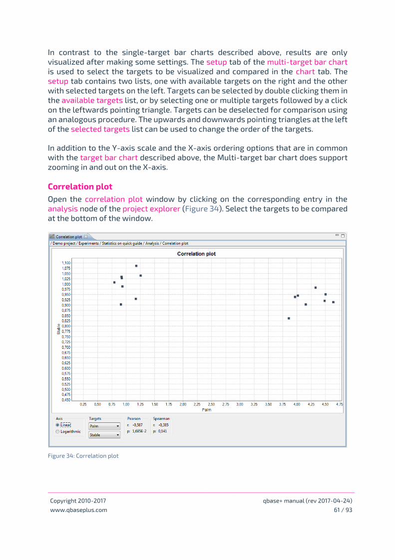
Copyright 2010-2017 qbase+ manual (rev 2017-04-24)
www.qbaseplus.com 61 / 93
In contrast to the single-target bar charts described above, results are only
visualized after making some settings. The setup tab of the multi-target bar chart
is used to select the targets to be visualized and compared in the chart tab. The
setup tab contains two lists, one with available targets on the right and the other
with selected targets on the left. Targets can be selected by double clicking them in
the available targets list, or by selecting one or multiple targets followed by a click
on the leftwards pointing triangle. Targets can be deselected for comparison using
an analogous procedure. The upwards and downwards pointing triangles at the left
of the selected targets list can be used to change the order of the targets.
In addition to the Y-axis scale and the X-axis ordering options that are in common
with the target bar chart described above, the Multi-target bar chart does support
zooming in and out on the X-axis.
Correlation plot
Open the correlation plot window by clicking on the corresponding entry in the
analysis node of the project explorer (Figure 34). Select the targets to be compared
at the bottom of the window.
Figure 34: Correlation plot

Copyright 2010-2017 qbase+ manual (rev 2017-04-24)
www.qbaseplus.com 62 / 93
Correlation coefficients (Pearson or Spearman) are only calculated on the samples
that are shown in the correlation plot (see Sample visibility settings). When the plot
is shown in logarithmic scale, the correlation coefficients are calculated based on
the 10log transformed results. As Spearman rank correlation is based on ranked
results, the correlation coefficients do not change in function of the axis scale.
We recommend Spearman rank correlation for a small sample size (< 24 data-
points) or for clearly non-normally distributed data. Pearson's correlation analysis
requires normally distributed data; as such, it is sensitive to outliers, especially
when the sample size is small. It is generally recommended to do statistics on log-
transformed gene expression levels.
Result table
Open the result table window by clicking on the corresponding entry in the analysis
node of the project explorer. The table shows the calibrated normalized relative
quantities (CNRQ values) for every sample-target combination, together with their
associated uncertainty expressed as standard errors. Sample-target combinations
without any value are not included in the experiment. ‘NaN’ is shown for
combinations that are included in the experiment, but for which no results could be
calculated – typically because of missing data.
Statistics
qbase+ has a built-in intuitive statistical wizard to perform commonly used
statistical tests on the results that are calculated in a single experiment, i.e. quality
controlled and rescaled (inter-run calibrated) normalized relative quantities (CNRQ
values). The stat module is specifically tailored towards the typical needs of
biologists performing qPCR analysis. This philosophy is reflected in a wizard based
approach that minimizes the use of statistical lingo, asks only minimal input from
the user, and provides the required information to guide the user to appropriate
statistical test and accompanying settings.
Importantly, the stat module is much more than a p-value generator; it also
calculates relevant values such as the mean value per sample subgroup or the fold
change (ratio) between 2 groups, always with accompanying 95% confidence
interval and graphics.
Using the statistical wizard
Prepare your data before launching the stat wizard by properly annotating your
experiment (including custom sample properties), performing basic relative
quantification analysis according to the appropriate settings and by thoroughly
evaluating the different built in quality controls. Start the wizard by clicking Stat
wizard ( ) in the project explorer tree on the left, under Analysis ( ) > Statistics (
). The wizard guides users to results in 4 easy steps.

Copyright 2010-2017 qbase+ manual (rev 2017-04-24)
www.qbaseplus.com 63 / 93
Specify the goal of your analysis
The first step in the wizard enables specification of the goal of your analysis (Figure
35). The selected goal guides the user to the statistical test that will be applied at
the end of the wizard.
Figure 35: Statistics wizard - step 1
The “Mean comparison” goal leads to:
• Unpaired t-test
• Paired t-test
• Mann-Whitney test
• Wilcoxon signed rank test
• One-way ANOVA
The “Target correlation” goal leads to:
• Pearson correlation
• Spearman correlation
The “Survival analysis” goal leads to:
• Cox proportional hazards

Copyright 2010-2017 qbase+ manual (rev 2017-04-24)
www.qbaseplus.com 64 / 93
Define sample groups
Here, the user either defines the sample groups that need to be compared, or
restricts the analysis to a subset of the samples. Such sample groups are based on
samples with identical sample property values (Figure 36). Consult the ‘Annotation’
chapter for more information on custom sample properties.
Figure 36: Statistics wizard - step 2
Select targets
Statistical analysis can be performed on a single target (gene), on multiple targets,
or on all targets measured in the experiment (excluding reference targets). If more
than one target is being analyzed, qbase+ automatically suggests performing a
multiple testing correction of the calculated p-values.
Make last settings
Technical questions with statistical terminology have been reduced to a minimum
while maintaining statistical validity by recognizing the nature of the data that is
being analyzed. For example, relative quantities that do not follow a log-normal
distribution should be log-transformed to make them suitable for parametric
analyses. Without user intervention, qbase+ will automatically logarithm transform
the results prior to doing stats.

Copyright 2010-2017 qbase+ manual (rev 2017-04-24)
www.qbaseplus.com 65 / 93
Figure 37: Statistics wizard - step 4
For a paired analysis (e.g. Paired t-test or Wilcoxon signed rank test), two sample
properties are required: a grouping property (similar to unpaired statistical
analyses) and a pairing property (unique to a paired analysis). The example below
describes the required sample properties for a hypothetical experiment in which
gene expression levels were measured in blood from 6 mice before and after
treatment with a given compound. The first column contains the sample names, the
second column contains the grouping property 'treatment' with values 'before' and
'after', the third column contains the pairing property 'mouse ID' with values
denoting the ID of the mice that will be used to identify the samples that belong
together, i.e. are paired and come from the same mouse. A pairing value can be a
number or a letter combination, and must be identical and unique for the pair.

Copyright 2010-2017 qbase+ manual (rev 2017-04-24)
www.qbaseplus.com 66 / 93
Table 1: Pairing properties
By progressing through the 4 steps in the wizard, the number of appropriate
statistical tests (shown on the right side) will decrease until only one test remains
(Figure 37) that will subsequently be used. At each step of the wizard, relevant
information and alerts are displayed at the bottom of the wizard.
Results
Each analysis is saved in the statistics ( ) section of the project explorer tree with
a unique name containing the statistical analysis performed followed by a serial
number. These results can be deleted, renamed and exported (CSV, XLS or XLSX file
type). Upon opening (double clicking) a stat result ( ) in the project explorer, results
are recalculated instantaneously. Hence, if data have changed, results will reflect
that change (e.g. more samples were added to the experiment, or calculation
settings were modified). Dramatic changes (e.g. removal of a target for which
results were previously calculated) can result in a conflict, whereby an alert will be
shown that results cannot be recalculated. In this situation, the user needs to
restart the wizard and complete a new analysis.
A stat result window contains 3 tabs at the bottom: the table contains the calculated
p-values and associated values, the chart tab provides a graphical representation
of the results, and the settings tab summarizes the input provided and options
selected using the stat wizard. Double clicking on a target or target pair in the table
tab may bring you to the corresponding graph, depending on the statistical test.
Each graph also has a dropdown list, for quick browsing through all results.

Copyright 2010-2017 qbase+ manual (rev 2017-04-24)
www.qbaseplus.com 67 / 93
Statistical result table and conditions of use
Unpaired t-test, Mann-Whitney
Column header Interpretation
Target Name of the target
The small icon in front of the target name can be
clicked to collapse / expand the details for that
target.
p p-value, multiple testing corrected (when selected)
Property Sample property used to define the subgroups
Comparison 2 values from property used to define the 2
subgroups
The direction of the comparison (A/B or B/A) can
be altered by changing the Target scaling options
in the Calculation parameters window. The
selected group will be used as denominator.
Ratio Fold change between nominator and denominator
subgroup
95% CI low lower value of the 95% confidence interval of the
ratio
95% CI high upper value of the 95% confidence interval of the
ratio
Value sample property value used to define one of the
subgroups
Mean mean value of the sample subgroup (value
depends on 'Target scaling' option)
95% CI low lower value of the 95% confidence interval of the
mean value
95% CI low upper value of the 95% confidence interval of the
mean value
Datapoints number of datapoints per subgroup
Table 2: Results for unpaired t-test and Mann-whitney test
Note 1: no equal variances are assumed in the unpaired t-test as Satterthwaite
approximation is used
Note 2: non-symmetrical CIs are obtained because statistical analysis are
performed on log transformed data
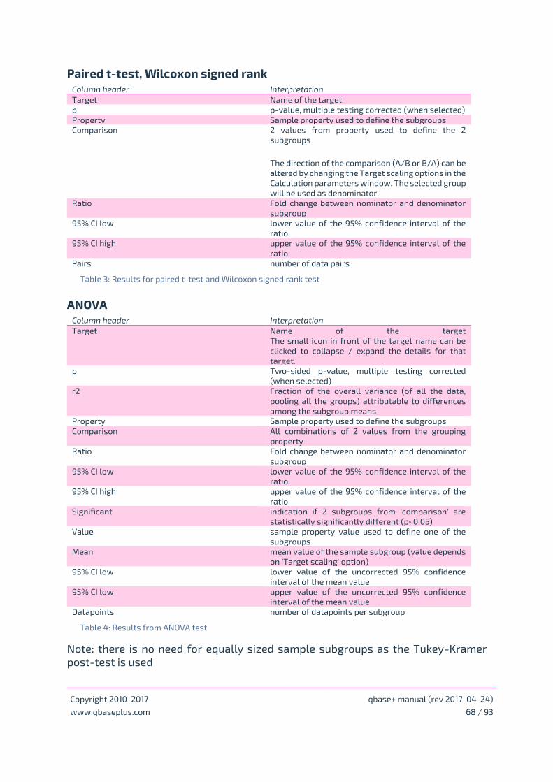
Copyright 2010-2017 qbase+ manual (rev 2017-04-24)
www.qbaseplus.com 68 / 93
Paired t-test, Wilcoxon signed rank
Column header Interpretation
Target Name of the target
p p-value, multiple testing corrected (when selected)
Property Sample property used to define the subgroups
Comparison 2 values from property used to define the 2
subgroups
The direction of the comparison (A/B or B/A) can be
altered by changing the Target scaling options in the
Calculation parameters window. The selected group
will be used as denominator.
Ratio Fold change between nominator and denominator
subgroup
95% CI low lower value of the 95% confidence interval of the
ratio
95% CI high upper value of the 95% confidence interval of the
ratio
Pairs number of data pairs
Table 3: Results for paired t-test and Wilcoxon signed rank test
ANOVA
Column header Interpretation
Target Name of the target
The small icon in front of the target name can be
clicked to collapse / expand the details for that
target.
p Two-sided p-value, multiple testing corrected
(when selected)
r2 Fraction of the overall variance (of all the data,
pooling all the groups) attributable to differences
among the subgroup means
Property Sample property used to define the subgroups
Comparison All combinations of 2 values from the grouping
property
Ratio Fold change between nominator and denominator
subgroup
95% CI low lower value of the 95% confidence interval of the
ratio
95% CI high upper value of the 95% confidence interval of the
ratio
Significant indication if 2 subgroups from 'comparison' are
statistically significantly different (p<0.05)
Value sample property value used to define one of the
subgroups
Mean mean value of the sample subgroup (value depends
on 'Target scaling' option)
95% CI low lower value of the uncorrected 95% confidence
interval of the mean value
95% CI low upper value of the uncorrected 95% confidence
interval of the mean value
Datapoints number of datapoints per subgroup
Table 4: Results from ANOVA test
Note: there is no need for equally sized sample subgroups as the Tukey-Kramer
post-test is used

Copyright 2010-2017 qbase+ manual (rev 2017-04-24)
www.qbaseplus.com 69 / 93
Spearman correlation, Pearson correlation
Column header Interpretation
Target X Name of the target in the X-axis
Target Y Name of the target in the Y-axis
r correlation coefficient
p p-value
Table 5: Results for correlation analysis
Note: switching target between X and Y axis has no effect on p and r value.
Cox proportionzal hazards
Column header Interpretation
Target Name of the target
p p-value
HR hazard ratio, increase (or decrease if HR < 1) in risk
per log10 unit (equals 10-fold difference) increase in
CNRQ value
95% CI low lower value of the 95% confidence interval of the HR
95% CI low upper value of the 95% confidence interval of the HR
Datapoints number of datapoints used in the Cox model
Table 6: Results for Cox proportional hazards analysis

Copyright 2010-2017 qbase+ manual (rev 2017-04-24)
www.qbaseplus.com 70 / 93
Statistical background
Calculations on logarithm transformed rescaled result table
As gene expression levels are typically log-normally distributed, all statistical
calculations are done on the log10 transformed CNRQ values (Hellemans and
Vandesompele, 2011). For easy interpretation of the statistical results, values are
re-transformed to linear scale by taking the anti-logarithm. The statistical results
are based on the rescaled results, hence, the mean values per subgroup (as well as
their respective 95% confidence intervals) will change in function of the target
scaling option selected in the project explorer tree (Settings > Calculation
parameters > Target scaling).
Of note, rescaling has no effect on the p-values and fold changes (ratio).
One-sided and two-sided p-values
If you know the direction of the observed effect (e.g. gene expression levels are
decreased after siRNA treatment) prior to generating the data and performing the
statistical test, you can use a one-sided p-value. In all other cases, a two-side p-
value is recommended. Note that if you selected a one-sided p-value and if the
direction is opposite to what you expected, then you need to adjust the p-value by
calculating 1-p (e.g. you expect a gene to be down regulated and therefore asked a
one-sided p-value; upon analysis, you observe a p-value of 0.075 but the gene
appears to be up regulated. Therefore, the true p-value is 0.925 (1-0.075)).
Multiple testing correction
It is highly recommended to correct the calculated p-values when testing multiple
hypotheses at the same time (e.g. when performing the same test for multiple
targets), in order to control the false positive rate. In qbase+, the false discovery
rate (FDR) multiple comparison method is implemented (Benjamini and Hochberg,
1995). This method guarantees that only 5% of all tests that yield a p-value smaller
than 0.05 are false positives.
While the FDR method is also applicable for correcting multiple ANOVA p-value
results, an additional multiple comparison post-test is implemented in each
individual ANOVA analysis when comparing the different subgroups. qbase+ uses
the Tukey-Kramer method to correct for the pairwise group comparisons in an
ANOVA test. Group comparisons that are statistically different in an ANOVA test
(corrected p-value < 0.05) are marked in the stat result table.
Multiple testing correction does not affect the size of the confidence intervals (CI);
the confidence intervals are in other words ‘uncorrected’ (this is also true for the
ANOVA CI). Consequently, results that appear significant based on their confidence
intervals (e.g. CI on ratio not overlapping 1) may have p-values larger than 0.05.
Copyright 2010-2017 qbase+ manual (rev 2017-04-24)
www.qbaseplus.com 71 / 93
Approximate and Exact p-values for non-parametric test
qbase+ calculates exact p-values for non-parametric tests when the sample size is
small and returns approximate p-values for large sample sizes (Spearman rank
correlation: > 6 pairs; Wilcoxon signed rank: > 50 pairs; Mann-Whitney: sum of the 2
groups > 50 datapoints with each group having > 10 datapoints).
Are the data coming from a log-normal distribution?
The sample size (N) and population distribution (log-normal or not) are both
important to select the proper statistical test. The following table helps with this
selection. In short, when the sample size is sufficiently large (typically two dozen or
24 datapoints), the choice of parametric or non-parametric test is irrelevant. A
parametric test can be safely used by relying on the central limit theorem that
states that the sample means follow a normal distribution when the sample size is
sufficiently large; a non-parametric test is sufficiently powerful when the sample
size is large.
For smaller sample sizes (N<24), a parametric test can be safely used if the
population distribution is log-normal (i.e. normally distributed when log-
transformed).
For sample sizes smaller than 24, but larger than a technical threshold (T value, see
further), a non-parametric test is always appropriate. When the underlying
population distribution is not known, qbase+ will apply a non-parametric test as
such a test is somewhat more conservative, resulting in slightly larger p-values.
However, when p<0.05, you can be more sure that there is a real difference.
For sample sizes smaller than the technical threshold T, there is only one valid
option, i.e. a parametric test in combination with the assumption of log-normality.
Non-parametric tests for sample sizes smaller than T will always result in a p-value
> 0.05. For a Wilcoxon signed rank test, there must be at least 6 pairs (T=6). For a
Mann-Whitney test, the sum of the sample sizes of the 2 groups must be at least 8
(T1 + T2 = 8).
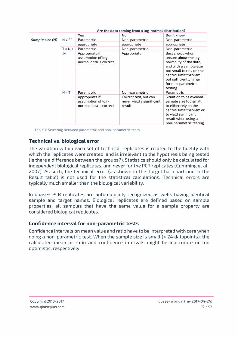
Copyright 2010-2017 qbase+ manual (rev 2017-04-24)
www.qbaseplus.com 72 / 93
Are the data coming from a log-normal distribution?
Yes No Don’t know
Sample size (N) N ≥ 24 Parametric Non-parametric Non-parametric
appropriate appropriate appropriate
T ≤ N <
24
Parametric Non-parametric Non-parametric
Appropriate if
assumption of log-
normal data is correct
Appropriate Best choice when
unsure about the log-
normality of the data,
and with a sample size
too small to rely on the
central limit theorem
but sufficiently large
for non-parametric
testing
N < T Parametric Non-parametric Parametric
Appropriate if
assumption of log-
normal data is correct
Correct test, but can
never yield a significant
result
Situation to be avoided.
Sample size too small
to either rely on the
central limit theorem or
to yield significant
result when using a
non-parametric testing
Table 7: Selecting between parametric and non-parametric tests
Technical vs. biological error
The variation within each set of technical replicates is related to the fidelity with
which the replicates were created, and is irrelevant to the hypothesis being tested
(is there a difference between the groups?). Statistics should only be calculated for
independent biological replicates, and never for the PCR replicates (Cumming et al.,
2007). As such, the technical error (as shown in the Target bar chart and in the
Result table) is not used for the statistical calculations. Technical errors are
typically much smaller than the biological variability.
In qbase+ PCR replicates are automatically recognized as wells having identical
sample and target names. Biological replicates are defined based on sample
properties: all samples that have the same value for a sample property are
considered biological replicates.
Confidence interval for non-parametric tests
Confidence intervals on mean value and ratio have to be interpreted with care when
doing a non-parametric test. When the sample size is small (< 24 datapoints), the
calculated mean or ratio and confidence intervals might be inaccurate or too
optimistic, respectively.

Copyright 2010-2017 qbase+ manual (rev 2017-04-24)
www.qbaseplus.com 73 / 93
Exports
Export Datasets and Tables
qbase+ has an extensive data export functionality. This chapter explains how raw
and analyzed data can exported out of qbase+. The softwares also allows easy
data-exchange between qbase+ users (.xml format) and is able to generate project
files in the RDML (Lefever et al., Nucleic Acids Res, 2009) file format. RDML is a
universal, open and XML based data exchange format recommended to be used
according to the MIQE guidelines (Bustin et al., Clin Chem, 2009).
The software is only able to export data from opened experiments. The export
wizard can be launched by clicking the export button ( ) in the command bar. The
first step in this wizard is the selection of the dataset that is to be exported.
Alternatively, the context menu of several elements in the project explorer
(samples, targets, replicates, reference target stability, amplification efficiencies,
normalization factors and results) can be used to export data.
Export Amplification Efficiencies
This export will generate a table (in .csv, .xls or .xlsx format) with for each target a
series of efficiency related information:
• computed and user defined E value, with E = efficiency +1 (with an E of 2
being perfect, indicating 100% efficiency)
• computed and user defined standard error on E
• the coefficient of determination (r²) for the regression of the standard curve
• the slope of the standard curve
• the Y-intercept of the standard curve (only relevant for known standard
curves with known quantities)
Export Experiment
qbase+ offers the possibility to export an entire experiment (.xml format) for easy
data-exchange between qbase+ users. Such an experiment can be easily imported
using the import function ( ) and by selecting the option ‘Import Experiment’.
Exchanging such .xml data files will not result in any loss of data, annotation or
settings.
Export Normalization Factors
This export will generate a table (in .csv, .xls or .xlsx format) with for each sample
its normalization factor. In case of reference gene normalization, the relative
quantities for the selected reference genes will be included in the export as well.
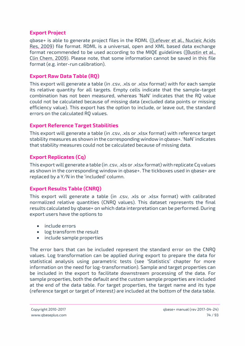
Copyright 2010-2017 qbase+ manual (rev 2017-04-24)
www.qbaseplus.com 74 / 93
Export Project
qbase+ is able to generate project files in the RDML ([Lefever et al., Nucleic Acids
Res, 2009) file format. RDML is a universal, open and XML based data exchange
format recommended to be used according to the MIQE guidelines ([Bustin et al.,
Clin Chem, 2009). Please note, that some information cannot be saved in this file
format (e.g. inter-run calibration).
Export Raw Data Table (RQ)
This export will generate a table (in .csv, .xls or .xlsx format) with for each sample
its relative quantity for all targets. Empty cells indicate that the sample-target
combination has not been measured, whereas ‘NaN’ indicates that the RQ value
could not be calculated because of missing data (excluded data points or missing
efficiency value). This export has the option to include, or leave out, the standard
errors on the calculated RQ values.
Export Reference Target Stabilities
This export will generate a table (in .csv, .xls or .xlsx format) with reference target
stability measures as shown in the corresponding window in qbase+. ‘NaN’ indicates
that stability measures could not be calculated because of missing data.
Export Replicates (Cq)
This export will generate a table (in .csv, .xls or .xlsx format) with replicate Cq values
as shown in the corresponding window in qbase+. The tickboxes used in qbase+ are
replaced by a Y/N in the ‘included’ column.
Export Results Table (CNRQ)
This export will generate a table (in .csv, .xls or .xlsx format) with calibrated
normalized relative quantities (CNRQ values). This dataset represents the final
results calculated by qbase+ on which data interpretation can be performed. During
export users have the options to
• include errors
• log transform the result
• include sample properties
The error bars that can be included represent the standard error on the CNRQ
values. Log transformation can be applied during export to prepare the data for
statistical analysis using parametric tests (see ‘Statistics’ chapter for more
information on the need for log-transformation). Sample and target properties can
be included in the export to facilitate downstream processing of the data. For
sample properties, both the default and the custom sample properties are included
at the end of the data table. For target properties, the target name and its type
(reference target or target of interest) are included at the bottom of the data table.
Copyright 2010-2017 qbase+ manual (rev 2017-04-24)
www.qbaseplus.com 75 / 93
Export Samples
This export will generate a table (in .csv, .xls or .xlsx format) with for each sample
information about their type, a description, quantity, custom normalization factor,
positive control quantity and a variable number of custom sample properties.
Export Targets
This export will generate a table (in .csv, .xls or .xlsx format) with for each target
information about its type: ‘REF’ for reference targets and ‘TOI’ for targets of
interest.
Export Statistics Results
This export will generate a table (in .csv, .xls or .xlsx format) with statistics results
for the selected test in a format similar to what is shown in the corresponding
window in qbase+. More information on the interpretation of this table is available
in the ‘Statistics’ chapter.
Export Figures
qbase+ charts can be copied for pasting in other applications, or be exported in any
of the following formats: .png, .jpg, .pdf or .svg. Both the copy and the export
functions are available as options in the context menu of selected graphs.

Copyright 2010-2017 qbase+ manual (rev 2017-04-24)
www.qbaseplus.com 76 / 93
Special applications
geNorm
geNorm analysis enables the selection of the optimal set of reference genes from a
series of tested candidate reference genes (Vandesompele et al., Genome Biology,
2002). The qbase+ implementation of geNorm provides five great benefits
compared to its predecessor in Microsoft Excel:
1. Calculation of relative quantities and geNorm analysis are combined in a
single program to speed up analysis. Previously, many manual pre-
calculations were needed.
2. Experiments with missing data are automatically processed in a way that has
the lowest impact on the overall analysis through intelligent retention of as
many data points as possible.
3. Whereas geNorm Excel could not distinguish the two most stably expressed
genes, qbase+’s geNorm now allows ranking of candidate reference genes
up to the single most stable gene.
4. Interpretation of a geNorm result is not always straightforward and
requires a certain level of expertise. To accommodate this, qbase+ now
includes an expert interpretation with recommendations on the number and
nature of genes to be used for optimal normalization as well as information
on the suitability of the selected genes.
• The geNorm implementation in qbase+ is at least 20 times faster than that
in Excel.
If your final experiment contains many samples, it is highly recommended to
perform a geNorm pilot experiment. Such a pilot experiment involves the analysis
of a set of candidate reference genes (preferentially more than 8, coming from
different pathways and belonging to different functional classes) on a
representative set of samples (typically 10 independent samples). Use the sample
maximization approach (Hellemans et al., Genome Biology, 2007) to avoid unwanted
technical variation that may interfere with proper geNorm analysis.
It is important that the samples are representative for the final experiment; if one
works with treated and untreated samples, or with different biological subgroups,
an equal number of samples from these subgroups should be studied.

Copyright 2010-2017 qbase+ manual (rev 2017-04-24)
www.qbaseplus.com 77 / 93
Import run data in a new empty experiment
In qbase+ qPCR run data are organized in experiments. To start data analysis, a new
empty experiment needs to be created. Right click on the project ( ) in the qbase+
project explorer tree in which you want to start a new experiment and click new
experiment. If needed, create a new project first in a similar way (New > Project). An
experiment name and description can be provided in the experiment properties
window.
qbase+ experiments contain data from one or more runs. Run data can be imported
by clicking the downward pointing arrow ( ) in the toolbar followed by the selection
of the import Run option.
Selection of normalization strategy and reference genes
qbase+ supports a range of different normalization procedures to suit the specific
needs of different types of experiments (premium license only). For a geNorm pilot
experiment it is required to apply the multiple reference target normalization
approach.
Open the settings node in the project explorer, double click on calculation
paramaters, and select the option reference target(s) (Figure 38).
Figure 38: Normalization strategy
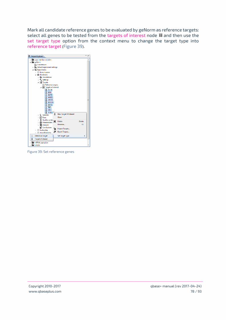
Copyright 2010-2017 qbase+ manual (rev 2017-04-24)
www.qbaseplus.com 78 / 93
Mark all candidate reference genes to be evaluated by geNorm as reference targets:
select all genes to be tested from the targets of interest node and then use the
set target type option from the context menu to change the target type into
reference target (Figure 39).
Figure 39: Set reference genes
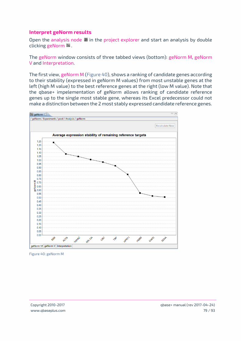
Copyright 2010-2017 qbase+ manual (rev 2017-04-24)
www.qbaseplus.com 79 / 93
Interpret geNorm results
Open the analysis node in the project explorer and start an analysis by double
clicking geNorm .
The geNorm window consists of three tabbed views (bottom): geNorm M, geNorm
V and Interpretation.
The first view, geNorm M (Figure 40), shows a ranking of candidate genes according
to their stability (expressed in geNorm M values) from most unstable genes at the
left (high M value) to the best reference genes at the right (low M value). Note that
the qbase+ impelementation of geNorm allows ranking of candidate reference
genes up to the single most stable gene, whereas its Excel predecessor could not
make a distinction between the 2 most stably expressed candidate reference genes.
Figure 40: geNorm M
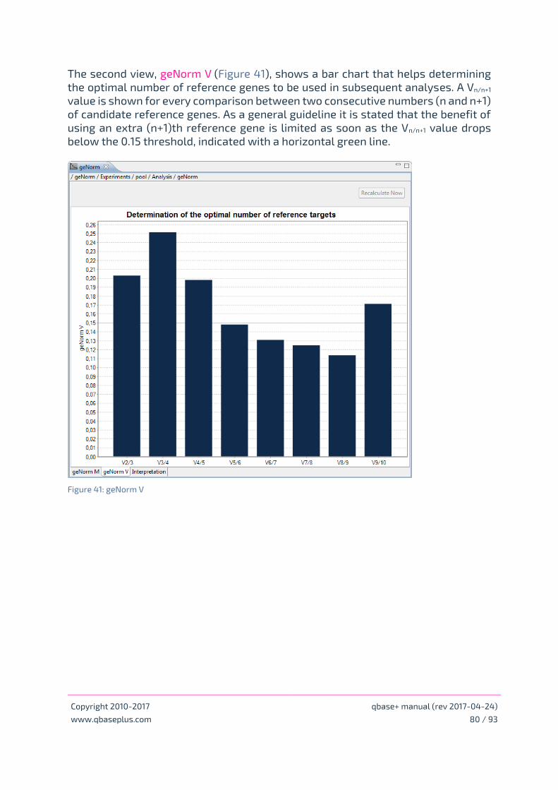
Copyright 2010-2017 qbase+ manual (rev 2017-04-24)
www.qbaseplus.com 80 / 93
The second view, geNorm V (Figure 41), shows a bar chart that helps determining
the optimal number of reference genes to be used in subsequent analyses. A Vn/n+1
value is shown for every comparison between two consecutive numbers (n and n+1)
of candidate reference genes. As a general guideline it is stated that the benefit of
using an extra (n+1)th reference gene is limited as soon as the Vn/n+1 value drops
below the 0.15 threshold, indicated with a horizontal green line.
Figure 41: geNorm V
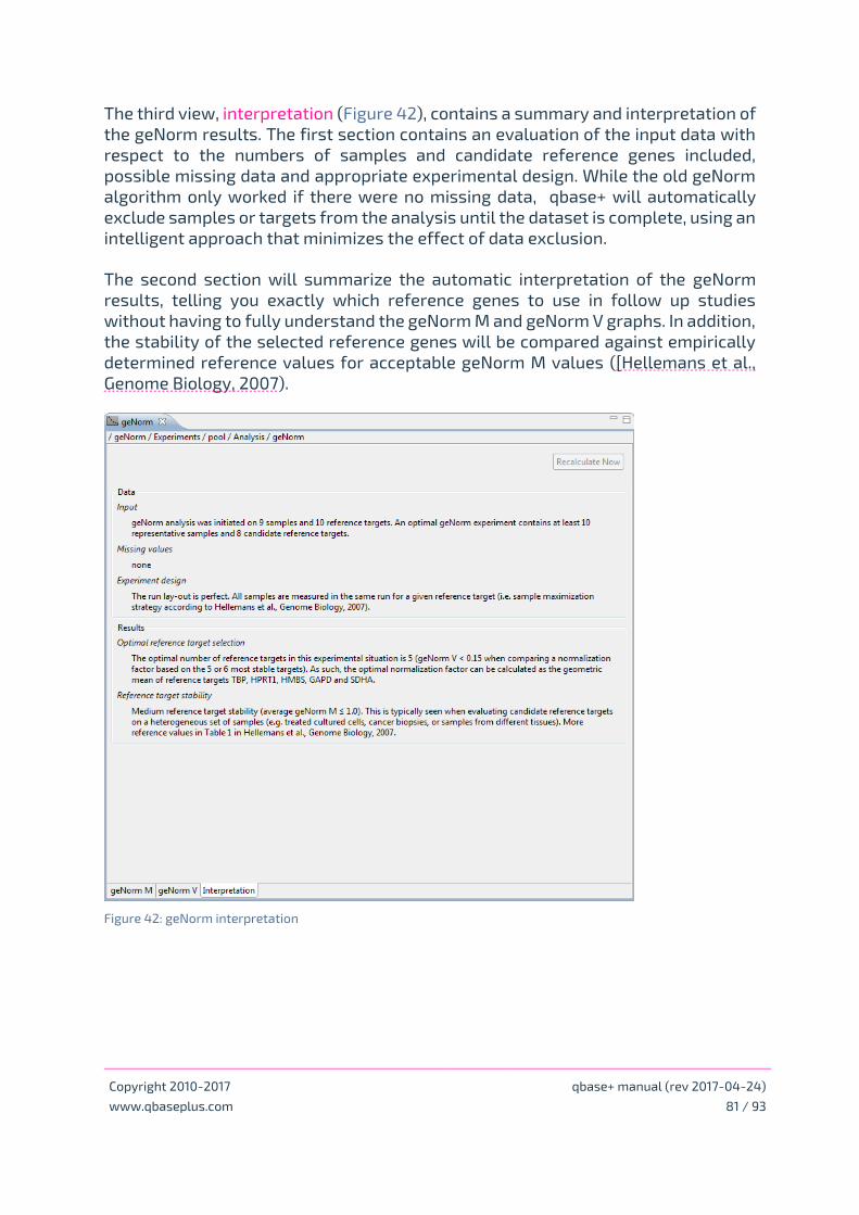
Copyright 2010-2017 qbase+ manual (rev 2017-04-24)
www.qbaseplus.com 81 / 93
The third view, interpretation (Figure 42), contains a summary and interpretation of
the geNorm results. The first section contains an evaluation of the input data with
respect to the numbers of samples and candidate reference genes included,
possible missing data and appropriate experimental design. While the old geNorm
algorithm only worked if there were no missing data, qbase+ will automatically
exclude samples or targets from the analysis until the dataset is complete, using an
intelligent approach that minimizes the effect of data exclusion.
The second section will summarize the automatic interpretation of the geNorm
results, telling you exactly which reference genes to use in follow up studies
without having to fully understand the geNorm M and geNorm V graphs. In addition,
the stability of the selected reference genes will be compared against empirically
determined reference values for acceptable geNorm M values ([Hellemans et al.,
Genome Biology, 2007).
Figure 42: geNorm interpretation
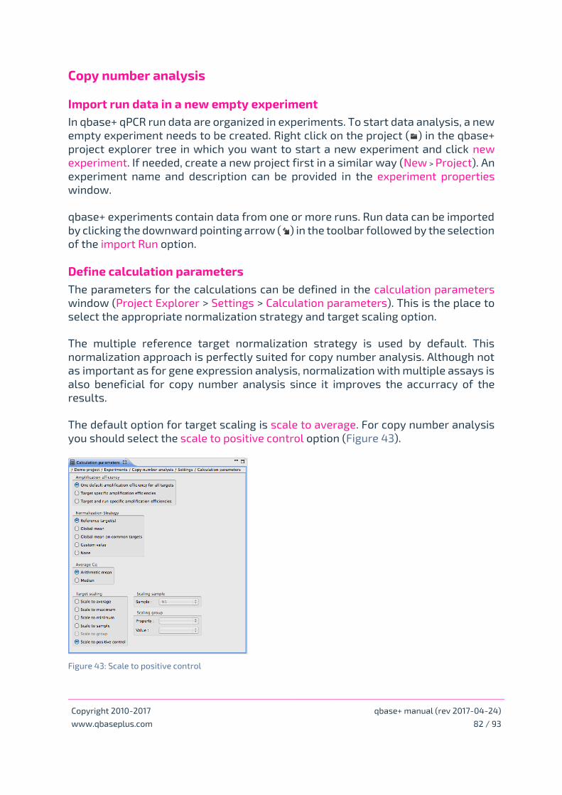
Copyright 2010-2017 qbase+ manual (rev 2017-04-24)
www.qbaseplus.com 82 / 93
Copy number analysis
Import run data in a new empty experiment
In qbase+ qPCR run data are organized in experiments. To start data analysis, a new
empty experiment needs to be created. Right click on the project ( ) in the qbase+
project explorer tree in which you want to start a new experiment and click new
experiment. If needed, create a new project first in a similar way (New > Project). An
experiment name and description can be provided in the experiment properties
window.
qbase+ experiments contain data from one or more runs. Run data can be imported
by clicking the downward pointing arrow ( ) in the toolbar followed by the selection
of the import Run option.
Define calculation parameters
The parameters for the calculations can be defined in the calculation parameters
window (Project Explorer > Settings > Calculation parameters). This is the place to
select the appropriate normalization strategy and target scaling option.
The multiple reference target normalization strategy is used by default. This
normalization approach is perfectly suited for copy number analysis. Although not
as important as for gene expression analysis, normalization with multiple assays is
also beneficial for copy number analysis since it improves the accurracy of the
results.
The default option for target scaling is scale to average. For copy number analysis
you should select the scale to positive control option (Figure 43).
Figure 43: Scale to positive control

Copyright 2010-2017 qbase+ manual (rev 2017-04-24)
www.qbaseplus.com 83 / 93
Define control samples
At least two types of control samples should be included in every qPCR-based copy
number analysis [D’haene et al., 2010]. As for all PCR based assays, a no template
control should be included to detect the presence of contaminating DNA. Specific
for qPCR-based copy number analysis, is the inclusion of reference samples
(positive controls) with a known copy number. These control samples are used as a
reference point (or calibrator) for determination of the true copy numbers. The
inclusion of multiple reference samples will result in more accurate results
(analogous to using multiple reference targets for more accurate normalization).
Positive and negative control samples should be appropriately labeled in the
sample list. Open the sample properties window for the control samples and
indicate the sample type (negative control or positive control). The positive control
option allows you to indicate a sample specific copy number (e.g. 2 for a normal
control or 1 for a deletion control) (Figure 44).
Figure 44: Quantity for positive controls
Please note that reference/calibrator samples with varying copy numbers can be
used to provide greater flexibility in reference sample choice and to allow known
deletions or duplications to be used both as a reference and as a point for quality
control on the ability of the assay to accurately call deletions or duplications. In this
example, we included three positive control samples with a known copy number: 2
normal controls (N1 and N2) and a deletion control (Positive).
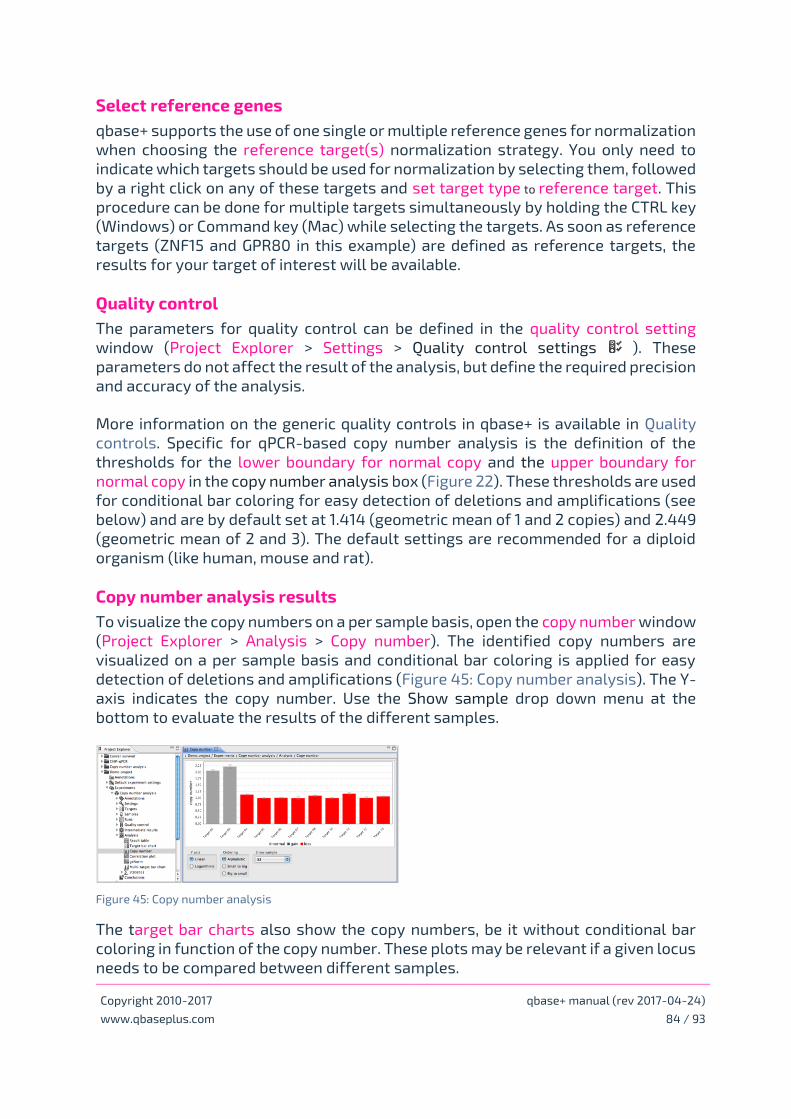
Copyright 2010-2017 qbase+ manual (rev 2017-04-24)
www.qbaseplus.com 84 / 93
Select reference genes
qbase+ supports the use of one single or multiple reference genes for normalization
when choosing the reference target(s) normalization strategy. You only need to
indicate which targets should be used for normalization by selecting them, followed
by a right click on any of these targets and set target type to reference target. This
procedure can be done for multiple targets simultaneously by holding the CTRL key
(Windows) or Command key (Mac) while selecting the targets. As soon as reference
targets (ZNF15 and GPR80 in this example) are defined as reference targets, the
results for your target of interest will be available.
Quality control
The parameters for quality control can be defined in the quality control setting
window (Project Explorer > Settings > Quality control settings ). These
parameters do not affect the result of the analysis, but define the required precision
and accuracy of the analysis.
More information on the generic quality controls in qbase+ is available in Quality
controls. Specific for qPCR-based copy number analysis is the definition of the
thresholds for the lower boundary for normal copy and the upper boundary for
normal copy in the copy number analysis box (Figure 22). These thresholds are used
for conditional bar coloring for easy detection of deletions and amplifications (see
below) and are by default set at 1.414 (geometric mean of 1 and 2 copies) and 2.449
(geometric mean of 2 and 3). The default settings are recommended for a diploid
organism (like human, mouse and rat).
Copy number analysis results
To visualize the copy numbers on a per sample basis, open the copy number window
(Project Explorer > Analysis > Copy number). The identified copy numbers are
visualized on a per sample basis and conditional bar coloring is applied for easy
detection of deletions and amplifications (Figure 45: Copy number analysis). The Y-
axis indicates the copy number. Use the Show sample drop down menu at the
bottom to evaluate the results of the different samples.
Figure 45: Copy number analysis
The target bar charts also show the copy numbers, be it without conditional bar
coloring in function of the copy number. These plots may be relevant if a given locus
needs to be compared between different samples.
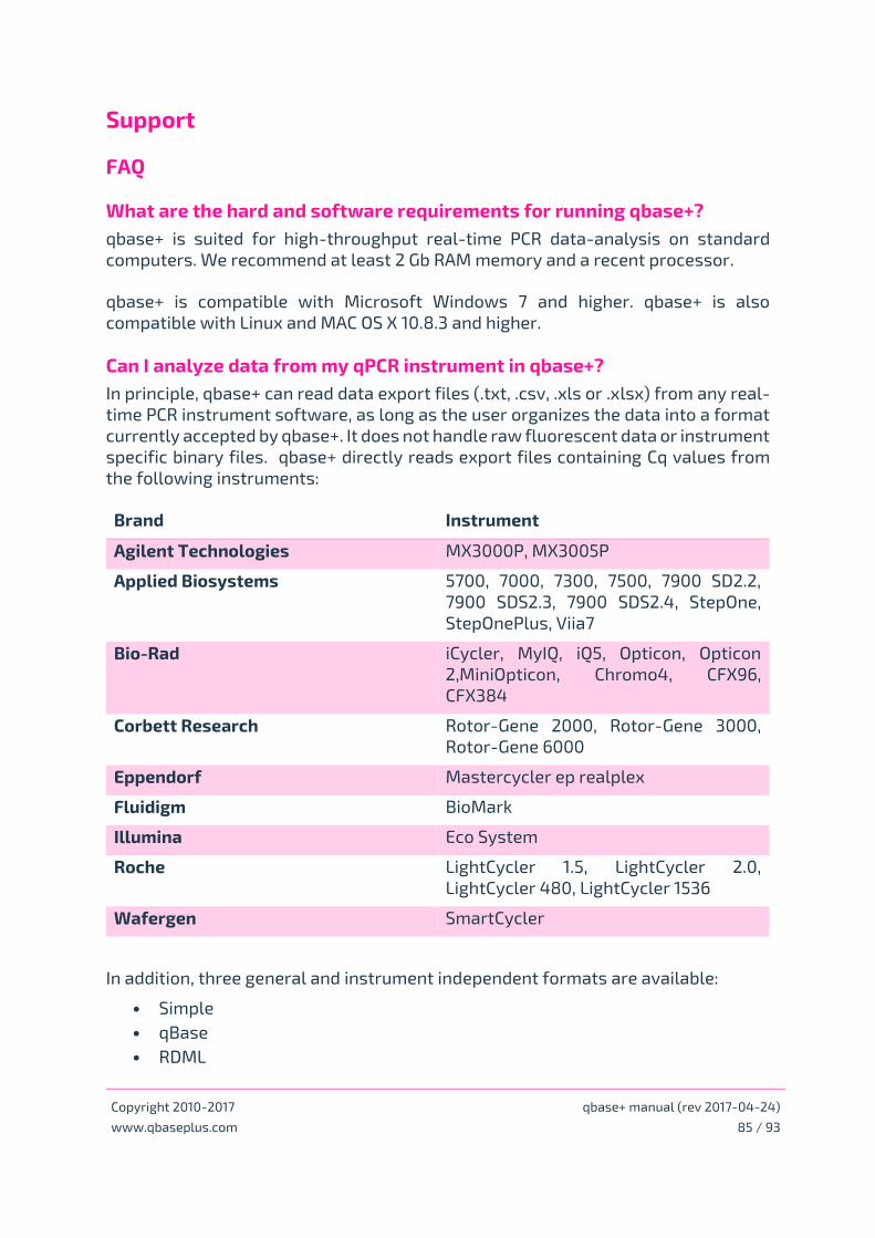
Copyright 2010-2017 qbase+ manual (rev 2017-04-24)
www.qbaseplus.com 85 / 93
Support
FAQ
What are the hard and software requirements for running qbase+?
qbase+ is suited for high-throughput real-time PCR data-analysis on standard
computers. We recommend at least 2 Gb RAM memory and a recent processor.
qbase+ is compatible with Microsoft Windows 7 and higher. qbase+ is also
compatible with Linux and MAC OS X 10.8.3 and higher.
Can I analyze data from my qPCR instrument in qbase+?
In principle, qbase+ can read data export files (.txt, .csv, .xls or .xlsx) from any real-
time PCR instrument software, as long as the user organizes the data into a format
currently accepted by qbase+. It does not handle raw fluorescent data or instrument
specific binary files. qbase+ directly reads export files containing Cq values from
the following instruments:
Brand Instrument
Agilent Technologies MX3000P, MX3005P
Applied Biosystems 5700, 7000, 7300, 7500, 7900 SD2.2,
7900 SDS2.3, 7900 SDS2.4, StepOne,
StepOnePlus, Viia7
Bio-Rad iCycler, MyIQ, iQ5, Opticon, Opticon
2,MiniOpticon, Chromo4, CFX96,
CFX384
Corbett Research Rotor-Gene 2000, Rotor-Gene 3000,
Rotor-Gene 6000
Eppendorf Mastercycler ep realplex
Fluidigm BioMark
Illumina Eco System
Roche LightCycler 1.5, LightCycler 2.0,
LightCycler 480, LightCycler 1536
Wafergen SmartCycler
In addition, three general and instrument independent formats are available:
• Simple
• qBase
• RDML

Copyright 2010-2017 qbase+ manual (rev 2017-04-24)
www.qbaseplus.com 86 / 93
What are the basic calculations in qbase+?
qbase+ uses a generalized model of the delta-delta-Ct approach, thereby
supporting the use of gene specific amplification efficiencies and normalization
with multiple reference genes. All formulas of this model are detailed in Hellemans
et al., Genome Biology, 2007
1. Conversion of Cq values into relative quantities (RQs).
1.1. Calculation of the average Cq value for PCR replicates.
1.2. The average Cq value is transformed into the RQ using the average Cq across
all samples for that given gene as a reference point, and a calculated or user
defined amplification efficiency.
2. Conversion of RQ values into normalized relative quantities (NRQs).
2.1. Calculation of the normalization factor (NF) for each sample is typically
based on the RQs of the reference genes for that sample. Alternative
normalization methods are available.
2.2. The NRQ is calculated by dividing the RQ by the sample specific NF.
3. Conversion of NRQ values into CNRQs (calibrated normalized relative quantities).
Only needed when expression levels for a given gene are compared between
samples measured in different runs. Inter-run calibration is based on
comparison of results for samples that have been measured for the same gene
in different plates, i.e. inter- run calibrators (IRC).
3.1. Calculation of the calibration factor (CF) for a given gene in a run based on
the RQs of the inter-run calibrators (IRCs)in that run.
3.2. The CNRQ is calculated by dividing the NRQ by the CF.
4. Final CNRQ or NRQ results can then be rescaled according to various user
preferences.
This only changes the scale of the data, but not the fold changes between the
samples. By default, expression levels are scaled to the average across all
samples. Alternatively, expression levels can be rescaled to the sample with the
lowest or highest expression, to a specific sample (e.g. untreated control), to the
average of a certain group (e.g. all control samples), etc.
What is the meaning of CNRQ value in the result table?
CNRQ = Calibrated Normalized Relative Quantity
If one does not perform inter-run calibration, then CNRQ equals NRQ (Normalized
Relative Quantity). This value represents the relative quantity (gene expression
level, copy number, …) between different samples for a given target (gene). It does
not have an absolute scale, and is only meaningful in comparison to values obtained
for other samples measured for that gene in the same experiment.

Copyright 2010-2017 qbase+ manual (rev 2017-04-24)
www.qbaseplus.com 87 / 93
Where is the calculate button?
By default, qbase+ will automatically recalculate on every change (selection of
reference genes, exclusion of replicates, changed settings, …). This approach offers
the best user experience for typical experiments, but may not be the best solution
for very large experiments that require too much computing time. In these cases, it
is best to disable the “Recalculate automatically” setting in the preferences window.
After having disabled this setting, a new icon is added to the command bar. Now,
results are only recalculated when clicking that button.
How do I save the changes to my experiments?
There is no need to save an experiment because qbase+ will save all the new data,
annotations, and other changes automatically in the background.
One exception to this approach is an update of text fields. These need to be
confirmed (ENTER or click on save icon) before the changes are applied and saved.
Unconfirmed changes can be recognised by the blue font (versus a black font for
saved text).
How is PCR efficiency calculated and used for relative quantification?
The gold standard method for PCR efficiency estimation is a serial dilution of
representative template (e.g. a mixture of RNA or cDNA from your samples). The PCR
efficiency can be calculated from the slope of a serial dilution as follows: PCR
efficiency= 10^(-1/slope) - 1. The formula to go from Cq values to relative quantities
is (E+1)^delta-Cq (hence 2^delta-Cq for an assay with 100% PCR efficiency).
In qbase+, users should provide the base of the exponential function as
amplification efficiency value for relative quantification if they want to correct for
target specific efficiency. The base number (E) is the efficiency value + 1, e.g. 1.95 for
95% efficiency (E value of 1.95).
Next to the gold standard method for PCR efficiency, there are a few algorithms
(from the large number out there) that provide an estimate of the PCR efficiency
based on a single amplification curve. Importantly, the calculated results should be
precise and accurate (and many algorithms fail in this respect). Hence, various
papers (see references below) point at the danger of using sample specific PCR
efficiencies based on a single amplification curve (or even replicate measurements).
The authors rather propose to average the sample specific efficiencies to obtain a
target (gene) specific efficiency. This is also what we recommend to our users.
LinRegPCR is a program that calculates Cq & efficiency values for fluorescent
amplification curves & exports data in RDML file format that can be directly
imported in qbase+.
References: Nordgård et al., Anal Biochem, 2006; Goll et al., BMC Bioinformatics,
2006; Karlen et al., BMC Bioinformatics, 2007.

Copyright 2010-2017 qbase+ manual (rev 2017-04-24)
www.qbaseplus.com 88 / 93
How to interpret the target bar chart?
The target bar chart represents the Normalized Relative Quantities (NRQ) or the
Calibrated Normalized Relative Quantities (CNRQ) values for all samples for a
specific target. By default qbase+ expresses the results as fold changes relative to
the average expression (NRQ) across all samples for that gene. If you want to make
your results relative to a control or control group, you should set the target scaling
correspondingly (in the Calculation Parameters window). This will make the relative
expression for you control (group) 1, and the results for your other samples are than
expressed as the fold change compared to your control (group).
How does qbase+ deal with replicates?
Technical (PCR) replicates
qbase+ automatically deals with technical replicates or repeated
measurements. PCR wells with an identical sample and target name are
recognized as technical replicates. At the very beginning of the calculation
workflow, the software averages the Cq values of all (non-empty) wells of a
replicate group. Outliers can be removed before calculations
Biological replicates
It’s also possible to define biological replicates. Custom sample properties
defining biological groups can be added as extra information to the samples
(Sample properties window). They enable statistical analysis and grouping of
results in bar charts.
Inter-run calibrators (IRCs)
Inter-run calibration is a calculation procedure to detect and remove inter-run
variation. The experimenter measures one or more identical samples for the
same target in different runs. These identical samples are called inter-run
calibrators (IRCs) and they are used to detect and correct inter-run variation.
To avoid interpretation of inter-run calibrators as technical replicates, they
should have a different sample name in the different runs (e.g. IRC1_a, IRC1_b,
...). Users should then indicate that a number of sample names actually refer to
the same biological sample that is used as an inter-run calibrator (e.g. both
IRC2_a and IRC2_b refer to the second inter-run calibrator, sample IRC2). This
procedure is known as setting the inter-run calibrators.
Copyright 2010-2017 qbase+ manual (rev 2017-04-24)
www.qbaseplus.com 89 / 93
What is inter-run calibration and how does it work?
Inter-run calibration is a calculation procedure to detect and remove inter-run
variation. The experimenter measures one or more identical samples in different
runs. These identical samples are called inter-run calibrators (IRCs) and they are
used to detect and correct inter-run variation.
Detailed information is available in Hellemans et al., Genome Biology, 2007.
qbase+ is the only software that
• allows inter-run calibration using more than one IRCs making it more
accurate
• performs inter-run calibration after normalization allowing the
experimenter to re-synthesize cDNA from the inter-run calibrator RNA
samples
• propagates the error introduced during the inter-run calibration procedure
To avoid interpretation of inter-run calibrators as technical replicates, they should
have a different sample name in the different runs (e.g. IRC1_a, IRC1_b, ...). Users
should then indicate that a number of sample names actually refer to the same
biological sample that is used as an inter-run calibrator (e.g. both IRC2_a and IRC2_b
refer to the second inter-run calibrator, sample IRC2). This procedure is known as
setting the inter-run calibrators.
When do I need IRC?
Two different experimental set-ups can be followed in a qPCR relative
quantification experiment.
Sample maximization method:
• As many samples as possible are analyzed in the same run. This means that
different targets should be analyzed in different runs if not enough free
wells are available to analyze them all in the same run.
• Preferred method because the experimenter is usually interested in
comparing the expression level of a particular gene between different
samples. The sample maximization method does not suffer from (often
underestimated) technical (run-to-run) variation between the samples.
Gene maximization set-up:
• Analyzes multiple targets in the same run, and spreads samples across runs
if required.
• Often used in commercial kits or in prospective studies.
Copyright 2010-2017 qbase+ manual (rev 2017-04-24)
www.qbaseplus.com 90 / 93
Whatever set-up is used, inter-run calibration is required to correct for possible
run-to-run variation whenever a target is screened for different samples across
multiple runs.
How to flag bad technical replicates based on a standard deviation
threshold?
qbase+ flags bad replicates based on a user defined maximum allowed difference
in Cq values (defined in the Experiment quality control settings).
There is a relation between the standard deviation and difference in Cq
(independent of the actual Cq values). In fact, the standard deviation increases 0.1
units per 0.14 cycle difference between duplicated reactions; similarly, the standard
deviation increases 0.07 units per 0.1 cycle difference between duplicated reactions.
Hence, if you want to flag bad duplicates that differ by more than 0.2 standard
deviations, you need to use a 0.28 cycle difference. For triplicates, a standard
deviation threshold of 0.1 means that the highest and lowest Cq value can only differ
by maximum 0.1 Cq values from the middle point.
How to exclude PCR replicates that do not meet quality control criteria?
qbase+ flags bad replicates based on a user defined maximum allowed difference
in Cq values (defined in the Experiment quality control settings), but does not
automatically exclude outliers. This means that the experimenter needs to decide
what to do with the failing replicates (in Replicates window).
In addition to the (default) arithmetic mean on replicated Cq value measurements,
qbase+ also supports the calculation of median Cq values (option in the Calculation
parameters window). The median Cq value represents a more robust measure than
the arithmetic mean when confronted with outliers and having at least 3 PCR
replicates. Median results (without outlier removal) are a good alternative to
arithmetic averages with outlier removal.
Why does qbase+ ask to log transform the data when exporting the
results table?
It is good practice to log transform the final gene expression results (i.e. the
normalized relative quantities), in order to make the data distribution more
symmetrical (as gene expression data is often log normally distributed). Together
with the Central Limit Theorem, this allows the use of parametric statistical tests
and calculations that rely on a distribution that resembles a normal distribution (e.g.
classic t-test, confidence intervals, Analysis of Variance).
Note that log transformations will not have an adverse effect on non-parametric
statistical tests.

Copyright 2010-2017 qbase+ manual (rev 2017-04-24)
www.qbaseplus.com 91 / 93
Does the statistical wizard perform a log transformation?
Yes. As gene expression levels (NRQs) are typically log-normally distributed, all
statistical calculations are done on the log transformed CNRQ values.
For easy interpretation of the statistical results, values are re-transformed to linear
scale by taking the anti-logarithm. The statistical results are based on the rescaled
results, hence, the mean values per subgroup (as well as their respective 95%
confidence intervals) will change in function of the target scaling option selected in
the Project explorer tree (Settings > Calculation parameters > Target scaling). Of
note, rescaling has no effect on the p-values and fold changes (ratio).
Where does qbase+ save my data?
All experimental data stored in qbase+ are collected in a workspace. The location of
the workspace on your computer can be verified in qbase+ > File > Switch
workspace. The workspace is part of your file system and can be included in your
backup procedures like any other file or folder.
To create a new workspace you can copy an existing workspace and give it a new
name. You can easily switch between workspaces (qbase+ > File > Switch
workspace). We do not recommend sharing workspaces on network drives since
concurrent use of a single workspace is not supported, and may result in corrupted
data.
When launching qbase+ for the first time after an upgrade from a previous version,
the workspace (collection of all experimental data stored in qbase+) will be
converted to a new data structure. A zipped backup copy will be generated in your
workspace that allows for a rollback to a previous version of qbase+.
What is the difference between Reference target stability and geNorm?
geNorm was developed to support selection of the best set of reference genes from
a list of measured candidate reference genes. It is typically applied to pilot studies
that are only meant to select reference genes.
The reference target stability quality control can be applied to verify whether the
selected reference genes allow for reliable normalization. This quality control can
be applied to all experiments in which at least two reference genes are included.
In both cases, the calculation of the M-value is based on the same principle,
described in (Vandesompele et al., Genome Biology, 2002). The geNorm algorithm
uses the M-value calculation in an iterative process to zoom in onto the most stably
expressed candidate reference genes.
Copyright 2010-2017 qbase+ manual (rev 2017-04-24)
www.qbaseplus.com 92 / 93
What is the difference between "M" and "geNorm M" in qbase+? How are
the calculations different?
The M-value calculations are identical and described in Vandesompele et al.,
Genome Biology, 2002. The M-value in the reference target stability window is
determined using all reference targets and hence reflects the relative stability of all
appointed reference genes in that particular experiment. This is typically the place
where you investigate if the previously validated reference genes in your
experiment are (still) good (on average 2-4 reference genes should ideally be used
for final normalization in a given experiment).
The geNorm M value (geNorm analysis) is slightly different as it denotes the
average M value of all remaining reference genes upon stepwise exclusion of the
most unstable reference gene (highest M value). For more details, see Figure 2 in
http://www.ncbi.nlm.nih.gov/pmc/articles/PMC126239/. The geNorm module is
typically used for assessing the stability of a large set (ideally 8 or more) of
candidate reference genes. This is what we call a geNorm pilot experiment.
What to expect when performing a geNorm analysis in qbase+?
geNorm is a popular algorithm to determine the most stable reference
(housekeeping) genes from a set of tested candidate reference genes in a sample
panel. This is what we call a geNorm pilot experiment. In brief, geNorm calculates
the gene expression stability measure M for a reference gene as the average
pairwise variation V for that gene with all other tested reference genes. Stepwise
exclusion of the gene with the highest M value allows ranking of the tested genes
according to their expression stability.
The underlying principles and calculations are described in Vandesompele et al.,
Genome Biology, 2002, Accurate normalization of real-time quantitative RT-PCR
data by geometric averaging of multiple internal reference genes
The results in qbase+:
• A first chart (genorm M) indicates the average expression stability value of
remaining reference genes at each step during stepwise exclusion of the
least stable reference gene. Starting from the least stable gene at the left,
the genes are ranked. (In the reference target stability window you see the
values based on the calculation including all ref genes).
• A second chart (genorm V) indicates the pairwise variation V between two
sequential normalization factors containing an increasing number of genes.
A large variation means that the added gene has a significant effect and
should preferably be included for calculation of a reliable normalization
factor. We propose 0.15 as a cut-off value; below 0.15 the inclusion of an
additional reference gene is not required. For example, if the V3/4 value is
0.22, then the normalization factor should preferably contain at least the 4

Copyright 2010-2017 qbase+ manual (rev 2017-04-24)
www.qbaseplus.com 93 / 93
best reference genes. Subsequently, if the V4/5 value is 0.14, then there’s no
real need to include a 5th gene in the normalization factor.
Note: Please bear in mind that the proposed 0.15 value must not be taken as
a too strict cut-off. The second graph is only intended to be guidance for
determination of the optimal number of reference genes. Sometimes, the
observed trend (of changing V values when using additional genes) can be
equally informative. Anyway, ‘just’ using the 3 best reference genes (and
ignoring this second graph) is in most cases a valid normalization strategy,
and results in much more accurate and reliable normalization compared to
the use of only one single reference gene."
• Expert report with recommendations on the number and identity of genes to
be used for optimal normalization as well as information on the relative
suitability of the selected genes.