publications - earth and space sciences at the university

A continuous record of intereruption velocitychange at Mount St. Helens from codawave interferometryA. J. Hotovec-Ellis1, J. Gomberg2, J. E. Vidale1, and K. C. Creager1

1Department of Earth and Space Sciences, University of Washington, Seattle, Washington, USA, 2U.S. Geological Survey,University of Washington, Seattle, Washington, USA

Abstract In September 2004, Mount St. Helens volcano erupted after nearly 18 years of quiescence.However, it is unclear from the limited geophysical observations when or if the magma chamber replenishedfollowing the 1980–1986 eruptions in the years before the 2004–2008 extrusive eruption. We use coda waveinterferometry with repeating earthquakes to measure small changes in the velocity structure of Mount St.Helens volcano that might indicate magmatic intrusion. By combining observations of relative velocity changesfrom many closely located earthquake sources, we solve for a continuous function of velocity changes withtime. We find that seasonal effects dominate the relative velocity changes. Seismicity rates and repeatingearthquake occurrence also vary seasonally; therefore, velocity changes and seismicity are likely modulated bysnow loading, fluid saturation, and/or changes in groundwater level. We estimate hydrologic effects impartstress changes on the order of tens of kilopascals within the upper 4 km, resulting in annual velocity variations of0.5 to 1%. The largest nonseasonal change is a decrease in velocity at the time of the deep Mw=6.8 Nisquallyearthquake. We find no systematic velocity changes during themost likely times of intrusions, consistent with alack of observable surface deformation. We conclude that if replenishing intrusions occurred, they did not alterseismic velocities where this technique is sensitive due to either their small size or the finite compressibility ofthemagma chamber. We interpret the observed velocity changes and shallow seasonal seismicity as a responseto small stress changes in a shallow, pressurized system.

1. Introduction

Mount St. Helens (MSH) is a dacite-andesite stratovolcano located in southwestern Washington State, famousfor its massive explosive eruption in 1980. When it erupted again in late 2004, it did so with less than 2 weeksof warning, which took the form of vigorous shallow earthquake swarms [Moran et al., 2008; Thelen et al.,2008], GPS-measured deflation [Dzurisin et al., 2008; Lisowski et al., 2008], and visible deformation of the craterglacier [Dzurisin et al., 2008]. Petrologic studies of the eventually extruded magma found it was likely sourcednear the top of the chamber (~5 km depth), largely degased, and similar to but chemically distinct fromprevious eruptions. This evidence can be interpreted as either due to tapping of a geochemically isolatedregion of the chamber or mixing with a fresh supply of low-gas dacite from depth [Pallister et al., 2008]. It isnot clear whether this magmawas introduced into the system before the end of the last eruption in 1986 or ifthe magma chamber was replenished during the intereruptive period. Distinguishing which of these twoprocesses occurred is important for anticipating what MSH, and volcanoes like it, may do in the future.

There are limited geophysical data to constrain what occurred in the subsurface during the 18 years since theend of the previous dome-building eruption in late 1986 (Figure 1). A permanent GPS station installed atJohnston Ridge Observatory (JRO1, Figure 2) in 1997 and radar interferograms [Poland and Lu, 2008] recordedno measurable deformation attributable to the volcano between at least 1992 and September 2004. Earliertrilateration and campaign GPS further concur that although some measurable inflation occurred between1982 and 1991, no measurable surface deformation occurred after [Dzurisin et al., 2008]. However, lack ofgeodetic evidence does not exclude the possibility that finite compressibility of the magma chamber couldoffset deformation due to an intrusion [Dzurisin et al., 2008; Mastin et al., 2008].

The most compelling evidence for magmatic intrusions during this time period is the occurrence of severaldeep (6–10 km depth) swarms of earthquakes [Moran, 1994]. The first burst of deeper seismicity occurredfrom 1987 to 1992. Focal mechanisms for these earthquakes were primarily strike slip, but with P axes

HOTOVEC-ELLIS ET AL. ©2014. American Geophysical Union. All Rights Reserved. 1

PUBLICATIONSJournal of Geophysical Research: Solid Earth

RESEARCH ARTICLE10.1002/2013JB010742

Key Points:• CWImeasurements combined to createcontinuous history of velocity change

• Velocities at MSH during this time per-iod are dominated by seasonal effects

• Nisqually earthquake produceddecrease in velocity; no intrusionsignal observed

Correspondence to:A. J. Hotovec-Ellis,[email protected]

Citation:Hotovec-Ellis, A. J., J. Gomberg, J. E.Vidale, and K. C. Creager (2014), Acontinuous record of intereruptionvelocity change at Mount St. Helensfrom coda wave interferometry,J. Geophys. Res. Solid Earth, 119,doi:10.1002/2013JB010742.

Received 4 OCT 2013Accepted 10 FEB 2014Accepted article online 15 FEB 2014

http://publications.agu.org/journals/

http://onlinelibrary.wiley.com/journal/10.1002/(ISSN)2169-9356

http://dx.doi.org/10.1002/2013JB010742

http://dx.doi.org/10.1002/2013JB010742

inconsistent with the regional trend. Moran [1994] modeled these focal mechanisms as an increase inpressure within a cylindrical magma chamber and interpreted the pressurization as being due to the sealingof the shallow conduit system, trapping exsolved magmatic gases. During this time, there was also a series ofshallow gas explosions following rain and/or snow storms, interpreted as the explosive release of thesetrapped gases when water penetrated a low-permeability cap [Mastin, 1994]. Two more bursts of deepseismicity occurred from 1994 to 1995 and from 1997 to 1998. Several fixed-wing gas flights were flownbetween June and September 1998, when seismicity was at its peak. The first flight recorded gas emissions of1900 t/d of CO2, but the subsequent flights recorded only trace amounts or 0 t/d [Gerlach et al., 2008]. Focalmechanisms of the deeper seismicity suggested another increase in pressure within the magma chamber.Hypocentral relocations of the seismicity by Musumeci et al. [2002] revealed that a large number of deeperearthquakes occur on at least two NE-SW striking, steeply dipping faults rather than being distributed aroundthe chamber. They further suggested that the southeastern fault had slip consistent with magma beingperiodically injected into a truncated dike on the northwest side of the fault (i.e., right-lateral motion to the

north of the chamber, left lateral to thesouth as the chamber expands).

The state of the shallow subsurface isalso relevant, as the overwhelmingmajority (>99%) of seismicity leadingup to and during the 2004–2008eruption occurred above 4 km depth[Moran et al., 2008], and the eruptionitself was potentially influenced by anabnormally wet late summer [Scottet al., 2008]. The aforementionedshallow explosions from 1989 to 1991,which often also followed intenserainfall events, and shallow (<4 kmdepth), seasonally modulated[Christiansen et al., 2005] seismicitysuggest that the system above themagma chamber was also pressurizedlong before 2004 and sensitive to theinflux of water and/or other smallpressure perturbations of tens of

0

3

6

9

12

Dep

th w

rt. d

atu

m (

km)

–3 0 3

Distance North (km)

b)0

3

6

9

12

Dep

th w

rt. d

atu

m (

km)

1988 1990 1992 1994 1996 1998 2000 2002 2004

Year

Ga)

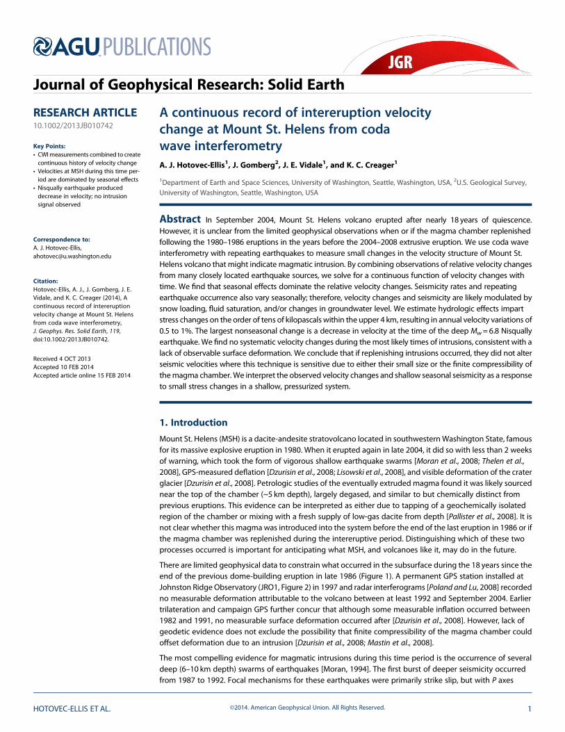
Figure 1. (a) Depth-time plot of well-located seismicity within 3 km of the dome (traveltime residual< .15 s, eight or morephases used, azimuthal gap ≤90º, and closest picked station within 5 km); coda wave interferometry was performed on allearthquakes in the catalog regardless of magnitude or location quality. Times of observed deformation from line lengthmeasurements (black bar), shallow explosions (arrows), and a gas emission (G) are also noted above the plot. Major swarmsof deeper seismicity are highlighted in gray and have been interpreted in other studies as a response to magmatic intru-sions. (b) Depth cross section through seismicity from south to north, centered on the dome. Depths are relative to a datum1.1 km above sea level, which is the average elevation of stations in the seismic network near MSH; surface elevation of MSHis plotted above for reference. Hypocenters below 6 km surround an aseismic magma chamber, denoted by a black ellipse.The geometry of this chamber is the same used to model strain in Figure 11 [from Lisowski, 2006].

–122.3˚ –122.2˚ –122.1˚

46.10˚

46.15˚

46.20˚

46.25˚

CDF

JUN

HSR

STD

SHW

FL2 EDMYEL

SEP

SOS

JRO1

748

553

777

1012

CDF

JUN

HSR

STD

SHW

FL2 EDMYEL

SEP

SOS

JRO1

748

553

777

1012

0 10km

SpiritLake

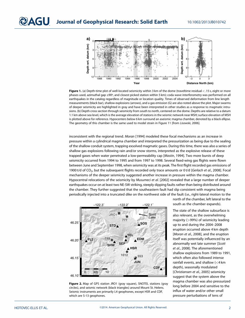
Figure 2. Map of GPS station JRO1 (gray square), SNOTEL stations (graycircles), and seismic network (black triangles) around Mount St. Helens.Seismic instruments are primarily L4 geophones, except HSR and CDF,which are S-13 geophones.

Journal of Geophysical Research: Solid Earth 10.1002/2013JB010742


kilopascal. Focal mechanisms of these shallow earthquakes further suggest a complex stress regime bestexplained by localized increases in pore pressure from water and/or magmatic gases [Lehto et al., 2013].

In this study, we use coda wave interferometry (CWI) of repeating earthquakes at MSH to measure smallchanges in seismic wave speed in an attempt to better resolve the timing of magma injection and thepressurization of the magmatic system, as well as the evolution of the shallow (<4 km) subsurface, includingthe conduit. Small (<1%) changes in seismic velocity have been observed at a handful of other volcanoesprior to eruptions [Ratdomopurbo and Poupinet, 1995; Wegler et al., 2006; Brenguier et al., 2008a], duringintrusive events [Ueno et al., 2012], in response to large earthquakes [Battaglia et al., 2012], and changes ingroundwater hydrology [Sens-Schönfelder and Wegler, 2006]. These observations and laboratory results [Grêtet al., 2006] suggest that seismic velocity, in particular S wave velocity [Snieder, 2002], is sensitive todeformation and the opening/closing of cracks due to changes in stress, fluid saturation, and temperature.

2. Data

Figure 2 is a map of the local seismic network surrounding Mount St. Helens between January 1987 andSeptember 2004. We use earthquakes that have epicenters and horizontal location uncertainty within 3 km ofthe volcano’s summit (i.e., a 3.4 km distant earthquake with 0.5 km horizontal uncertainty would be included)and depths between 0 and 12 km relative to the datum of the local velocity model, approximately 1.1 kmabove sea level (Figure 1b). This area comprises the majority of located seismicity in the MSH vicinity relatedto the volcano. Seismicity beneath the volcano between 1 and 4 km depth is persistent across the nearly18 year time span, whereas seismicity between 4 and 10 km mostly occurred in the three large swarms(Figure 1a). The earthquakes that we use in this study are cataloged and located by the Pacific NorthwestSeismic Network (PNSN), using a network of Mark L4-C and Geotech S-13 single component, short-period,analog instruments operated by the PNSN and Cascades Volcano Observatory. During this time, the networkconfiguration changed little, but instruments and VCO units were often replaced as part of normal stationmaintenance. Data from these stations were telemetered by radio to the PNSN in Seattle, WA. Until January2002, only triggered data were saved, limiting the ability to study this time period with continuous methodssuch as ambient noise interferometry.

3. Application of Coda Wave Interferometry

Seismic velocities are dependent on the physical properties of thematerials throughwhich the seismic wavestravel so that changes in these properties will produce a change in wave speed. Recent advances in theoryand signal processing have allowed seismologists to observe small spatiotemporal changes in seismicvelocities on the order of less than 0.1% by capitalizing on signals ordinarily discarded as noise. Onetechnique for identifying velocity change is coda wave interferometry (CWI), wherein the codas of repeatingearthquakes (also called repeaters, families, doublets, or multiplets) are compared. CWI operates under thetheory that the seismic coda of two colocated earthquakes is a summation of multiply-scattered waves, andsmall changes in either the source or medium will affect how the scattered waves sum at the station andtherefore alter the resulting waveform [e.g., Snieder, 2006]. The coda responds in distinct and predictableways to different kinds of changes in the medium. For example, consider a widespread and uniform decreasein wave speed that occurs between the times of two colocated earthquakes with the same focal mechanism.Coda waves from the second earthquake will arrive with increasing delay as the waves travel a longereffective distance through the slower medium by multiple scattering [e.g., Grêt et al., 2006]. CWI measures anapparent velocity change, which is the average relative velocity change in the volume through which thecoda waves propagate. It provides a lower bound on the maximum change, especially if the change isconcentrated and compact. In the case of a localized change, coda waves are most sensitive to velocityperturbations in an ellipse with foci at the source and receiver locations but then increasingly less sensitiveoutside of that depending on the strength of scattering, frequency, and time lag [Pacheco and Snieder, 2005].

A change in seismic velocity is distinguishable from a change in source location, source mechanism, orscatterer location in that these other types of changes do not produce increasing lag with time for codawaves [Snieder, 2006]. For example, a change in location will alter coda wave paths, lengthening some andshortening others, but on average, the traveltimes will be the same, and the slope of lag with time will be



zero. Although on average the slopefrom these other changes will be zero,they still alter the waveform andintroduce uncertainty in the calculationof relative velocity change differencebetween earthquake pairs.

CWI is ideally suited for use in volcanicsettings because repeatingearthquakes are commonplace atvolcanoes [e.g., Thelen et al., 2011],sometimes even during noneruptivephases [Saccorotti et al., 2007;Petersen, 2007; Carmona et al., 2010;Massin et al., 2013], and theheterogeneity of the subsurfaceprovides ample scattering. To findpairs of repeating earthquakes atMSH, we cross-correlate the entire18 year catalog of 1–10Hz band-passed waveforms on individualstations in a window 0.1 s before to2.4 s after the analyst-picked P wavearrival, or the expected P wave arrivalbased on the locations of theearthquake and station in the absenceof a pick. For each individual station, ifthe waveforms in this window

correlate above a normalized cross-correlation coefficient (CCC) of 0.8, we consider the two earthquakes tobe a possible repeating pair and realign the waveforms to the time of maximum correlation. Using theseparameters, we find that earthquakes with at least onematching event account for approximately 40% of thecatalog, with time gaps between some pairs of up to 10 years, but on average 1 year or less.

We then process each pair of repeating earthquakes using the doublet method of Snieder et al. [2002] todetermine velocity changes. For each pair of repeating events we divide the two waveforms intononoverlapping windows of 0.5 s length and calculate the CCC and lag for each window. We calculatethe expected S wave arrival based on the earthquakes’ location using the “S3” PNSN 1-D velocity model andVp/Vs= 1.78 and only consider windows after that arrival as being part of the coda. If there are at least fivewindows in the coda that have CCC above 0.65, we fit a straight line to those lags (Figure 3). The slope of thisline defines the relative velocity change, under the assumption that the change occurs uniformly throughoutthe entire contributing volume [Snieder, 2006]. This method is limited to velocity changes less than ~2 or 3%,as greater lags will reduce more windows below our 0.65 CCC cutoff. Clipping may also reduce the CCC, butonly affects a small portion of our data set. We also attempt to account for slight differences in location ofscatters, hypocenter, focal mechanism, and/or magnitude between the two earthquakes [e.g., Kanu et al.,2013] by only keeping pairs where the slope is well resolved and the standard deviation of the lags to thelinear regression is less than 0.01 s. Although in theory the technique is precise to 0.01 or 0.02%, we estimatethat our error for any given pair is closer to 0.1%. This is based on the standard deviation of velocitychanges for pairs less than 10 days apart, where we expect the change on this timescale to be close to zero.This process is repeated for all possible earthquake pairs for each station out to 15 km distance from thesummit of MSH.

Using the above procedure, we calculated relative velocity changes for thousands of event pairs separated bydays to years. In reality, the relative velocity change is a function of both time and space, but at MSH we donot have the network density to fully resolve the spatial extent of our observed velocity changes. Therefore,in this paper we only solve at each station for the average velocity change with time within the volumethrough which the coda waves travel. Because different families of earthquakes occur near each other (within

0 2 4 6 8 10

Time since first arrival (s)

0

50

–1

–0.5

0

0.5

Am

plit

ud

eL

ag (

ms)

75

25

–25

P S (expected)

Figure 3. (top) Example of two earthquakes recorded at HSR that correlatewell in the early waveform but decorrelate in the coda. S wave was notpicked on either earthquake, so expected arrival time to station is estimatedusing the PNSN S3 velocitymodel. (bottom) Lag and similarity of black-to-graywaveform within nonoverlapping, 0.5 s windows, plotted as circles at thecenter of the time window and lag time to maximum correlation. Unshadedregion between dotted lines denotes time window used to calculate slope oflags for velocity measurement; unfilled circles indicate windows where theCCC was below the 0.65 cutoff and were not used to determine slope. Thisslope corresponds to a relative decrease in velocity of 0.68%.



a few kilometers or less) and sample much of the same volume, we combine observations frommany nearbyearthquakes into a single velocity-change chronology.

Relative velocity changes are often compared for pairs of doublets across an abrupt known geophysicalevent, such as a large earthquake [Poupinet et al., 1984; Nakamura et al., 2002; Pandolfi et al., 2006; Li et al.,2007; Rubenstein et al., 2007; Battaglia et al., 2012]. In this paper we instead assume that there is somecontinuous function of velocity with time and that each pair of earthquakes is sampling the differencebetween the velocities at those two times. We solve for the continuous function of velocity change that fits allthe pairs of observed differential changes by a simple linear least squares inversion. The forward problem forany pair of earthquakes at times ti and tj is simply

dij ¼ γ tj� �� γ tið Þ (1)

in which dij is the observed relative velocity change and γ(t) is the continuous function of relative velocitychange with time for which we intend to solve. We discretize the function γ(t) evenly in time with a spacing ofonce every 10 days, i.e., the shortest amount of time we allow velocity to change over and linearly interpolatethe function between each point. Therefore,

γ tið Þ ¼ γ tkð Þ þ γ tlð Þ � γ tkð Þð Þ ti � tktl � tk

(2)

where k and l are the indices of γ on either side of ti. Solving for γ is highly unstable because the problem is illconditioned, so we are forced to regularize the inversion. We have chosen a combination of first- and second-order Tikhonov regularization (i.e., minimizing the first and second derivatives of the solution to favor asolution that varies slowly and smoothly) with equal weight and choose the solution with the best trade-offbetween roughness and misfit. Additionally, the mean is set to zero to further stabilize the inversion, as thereis no constraint on the absolute velocity.

4. Inversion Results

Before we apply the inversion to real data, we can test how well it can resolve known functions of velocitychange given the uneven sampling times from our real data. We have tested how well the inversion resolvesno change, a linear increase, a series of step functions, and a sinusoidal function in the presence of Gaussiannoise with standard deviation of 0.1%, our calculated error. Figure 4 shows what kinds of changes areresolvable when sampling a known continuous function at the times of earthquake pairs at station HSR,which has an average number of pairs but highly uneven sampling with time (i.e., repeating earthquakesoccur more commonly during autumn than spring, discussed later). The primary discrepancies betweenthe known input and the inversion result occur for times when the data are sparse, as expected. For this

1988 1990 1992 1994 1996 1998 2000 2002 2004

1988 1990 1992 1994 1996 1998 2000 2002 2004

1988 1990 1992 1994 1996 1998 2000 2002 2004

1988 1990 1992 1994 1996 1998 2000 2002 2004

–1.0

–0.5

0

0.5

1.0

–1.0

–0.5

0

0.5

1.0

–1.0

–0.5

0

0.5

1.0

–1.0

–0.5

0

0.5

1.0

d)c)

b)a)

Figure 4. Tests of how well our inversion is able to recover a known function of velocity change (gray line) in the presenceof Gaussian noise with standard deviation 0.1% dv/v and using the distribution of pairs at station HSR. The inverted solution(black line) has the best trade-off betweenmisfit and smoothness. (a) A slope of 0.01%/yr with no other changes, (b) a seriesof small step functions, (c) a random spline function, and (d) the sum of two sinusoids (periods of 0.5 and 1 year) and adifferent series of step functions function than Figure 4b. Raw data points are plotted around the solution in gray.



level of noise, the minimum resolvable step in velocity is ~0.2% and the minimum resolvable slope is~0.01%/yr. Sinusoidal signals are well resolved where there are data and are not an artifact of unevenearthquake repetition.

For the first inversion involving real data, we incorporate only pairs with depths less than 4 km, which iswhere most seismicity occurs, and we can expect good temporal resolution. Figure 5 shows the result of theinversion for the six most densely sampled and reliable stations. Although there are some time periods

Figure 5. (a) Inversion results for shallow (<4 km; black line, dashed where solution ill constrained) earthquake pairs only.Gray dots represent the times and relative velocity changes of individual pairs of observations. For a single earthquake pair,one dot is plotted at the time of the first earthquake, the other at the time of the second, and their vertical separation is theobserved velocity change between them. Pairs are plotted around the final solution such that if one dot is above thesolution, the other is an equal distance below it. The dots serve to illustrate the temporal density of data, as well asuncertainty in the continuous solution. (b) Comparison of inversion solution using shallow (same as in Figure 5a) and deep(>4 km; gray line, not plotted where ill constrained) earthquake pairs separately for two representative stations. Solutionsfor deep and shallow source earthquakes are similar in timing and amplitude, indicating that the coda waves from bothdepth subsets are sampling similar, presumably shallow volumes. Vertical gray line in both plots corresponds to the date ofM6.8 Nisqually earthquake. Results for stations SEP, YEL, EDM, and SOS are not plotted because there were an insufficientnumber of pairs to produce a stable inversion.



during which the solution is not well resolved, there is a strong annual cyclicity in the relative velocity changefor most of the stations. The Fourier transform of the velocity change on the nearest four stations has a strongpeak near 365 days, with a secondary peak around 183 days, indicating that the changes are seasonal. Sincewe aremore interested in velocity changes due to changes within the volcano itself, we have also inverted forvelocity change using a subset of earthquakes in the depth range 4 to 10 km, where we expected thatchanges from the magma chamber could be more visible due to a deeper source and sampling volume.Although the seismicity is more clustered in time, there are pairs of repeating earthquakes that span the gapsbetween swarms. Figure 5b also shows the remarkable similarity between relative velocity changes for the1 to 4 km and 4 to 10 km depth ranges and demonstrates that seasonal velocity changes are stronger thanany other signal from within the volcano for the entire depth range we consider. The similarity in amplitudeof the annual velocity changes for both subsets further suggests that our coda waves are primarily composedof surface waves sampling the shallow subsurface, consistent with our 1–10Hz band pass.

5. Seismicity Rate and Seasonal Repeaters

We observe a greater rate of repeating earthquakes during summer than winter when we include theentire catalog regardless of magnitude. Christiansen et al. [2005] found that M1.5+ earthquakes at MSH arestatistically more common between July and October than during the rest of the year. There is still a possibilitythat this is in part an artifact of an incomplete catalog due to station health during the winter. Christiansen et al.[2005] attribute the increased seismicity to reduced normal stress from snow unloading and/or increased porepressure of between 8 and 64 kPa from a rise in groundwater level by pore pressure diffusion.

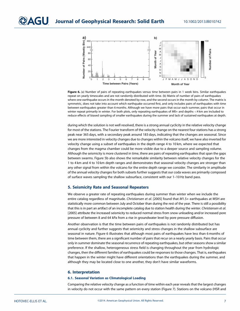
Another observation is that the time between pairs of earthquakes is not randomly distributed but hasannual cyclicity and further suggests that seismicity and stress changes in the shallow subsurface areseasonal in nature. Figure 6 illustrates that although most pairs of earthquakes have less than 6months oftime between them, there are a significant number of pairs that recur on a nearly yearly basis. Pairs that occuronly in summer dominate the seasonal recurrence of repeating earthquakes, but other seasons show a similarpreference. If the shallow, heterogeneous stress field is changing throughout the year from hydrologicchanges, then the different families of earthquakes could be responses to those changes. That is, earthquakesthat happen in the winter might have different orientations than the earthquakes during the summer, andalthough they may be located close to one another, they don’t have similar waveforms.

6. Interpretation6.1. Seasonal Variation as Climatological Loading

Comparing the relative velocity change as a function of time within each year reveals that the largest changesin velocity do not occur with the same pattern on every station (Figure 7). Stations on the volcano (HSR and

0 1 2 3 4 5 6 7 8 9 100

20

40

60

80

440

460

Nu

mb

er o

f P

airs

(W

eekl

y B

in)

Time between Pairs (Years)

Mo

nth

of Y

ear

Month of Year

Nu

mb

er o

f P

airs

JFMAMJJASOND

J F M A M J J A S O N D0

100b)a)

Figure 6. (a) Number of pairs of repeating earthquakes versus time between pairs in 1 week bins. Similar earthquakesrepeat on yearly timescales and are not randomly distributed with time. (b) Matrix of number of pairs of earthquakeswhere one earthquake occurs in the month denoted by row, and the second occurs in the month by column. The matrix issymmetric, does not take into account which earthquake occurred first, and only includes pairs of earthquakes with timebetween earthquakes greater than 6months. Although we have more pairs that occur each summer, pairs that occur inwinter repeat primarily in winter. For both plots, only repeating earthquakes of M0+ and depths <4 km are included toreduce effects of biased sampling of smaller earthquakes during the summer and lack of sustained earthquakes at depth.



SHW) have the highest relativevelocity changes in the spring months(March through May), while stationsoff the volcano (STD and JUN) havehighest changes in the late summerand early autumn (August throughOctober). Although less obvious, thetiming of the secondary peak forstations on the volcano aligns with theprimary peak for stations off thevolcano, and vice versa. To test howwell the differences between stationsare actually resolved by the inversion,we can compare the reduced chi-

square misfit χ2red� �

for the data at each

station with various velocity changemodels, γ(t). For example, a χ2red valuecalculated for the data from HSR andmodel from JUN of close to 1 wouldindicate that the model fits the datawithin the measurement uncertaintiesand accounts for the number of degreesof freedom. Table 1 summarizes thevalues of χ2red for data from the six beststations and models with no velocitychange, the best model for that station,HSR’s best model, JUN’s best model,and a model using data from all stationsin the same inversion. Perhapsunsurprisingly, using the model of JUNwith the data from HSR (and vice versa)results in a significant increase in themisfit, even more than the assumptionof zero change. We conclude that themodels of velocity change are uniqueand resolvable from each other.

Given that the difference inamplitudes between stations isresolvable, the differences most likelyrepresent different processes to whichstations have varying sensitivity withan ~6month offset and recurrenceinterval of 1 year. The high relativevelocity in March corresponds to thepeak annual snowpack, which wehave verified using four SNOTELstations in the Mount St. Helensvicinity (Figure 2) and would act toincrease the velocity by closing cracksdue to increased surface loading. Thegeneral shape of the snowpack curve(Figure 7) corresponds to the velocitiesat stations nearest the volcano (HSR

3445

3435

3445

3435

0

5

10

15

20

0

5

10

15

20

Sn

ow

Lo

ad (

kPa)

Sn

ow

Lo

ad (

kPa)

Lak

e E

leva

tio

n (

ft)

Lak

e E

leva

tio

n (

ft)

% R

elat

ive

Vel

oci

ty C

han

ge

Month of YearJ F M A M J J A S O N D

J F M A M J J A S O N D



–1.0

–0.5

0

0.5

1.0

–1.0

–0.5

0

0.5

1.0

–1.0

–0.5

0

0.5

1.0

–1.0

–0.5

0

0.5

1.0

JUN

STD

SHW

HSR

Figure 7. Velocity as a function of month of year, demeaned raw solu-tions in light gray and average in thicker black. Dashed line correspondsto average yearly snow load at SNOTEL station 748 in Sheep Canyon.Dotted line corresponds to average lake elevation at Spirit Lake, plottedwith an inverted y axis to better illustrate the anticorrelation. Shaded areadenotes months of the year with increased shallow seismicity fromChristiansen et al. [2005].



and SHW) with nearly zero lag. Also, HSR and SHW would receive more snow than JUN and STD due to theirelevation, and the relatively slower velocities in spring 1996 that occurred during a year with lower snowpackfurther suggest a causal relationship (Figure 8a).

The later peak in relative velocity in September corresponds to times when earthquakes occur morefrequently. It seems to us an unlikely coincidence that increased velocity and earthquakes occur during thesame time of year. One possibility is that an increase in the height of the groundwater table increases porepressures and reduces local effective normal forces, resulting in more frequent earthquakes. In addition, anincrease in the height of the groundwater table could increase velocities by closing cracks due to the weightof the water, similar to snow pack, or through poroelastic effects. Although no direct measures of thegroundwater table are available in the area, lake elevation data from Spirit Lake may be used as a proxy andconstraint on groundwater models. Simple hydrologic modeling by Christiansen et al. [2005] indicates thatthe groundwater level change is on the order of 1 to 9m. The timing of the maximum highs in modeledgroundwater levels qualitatively coincides with the onset of increased seismicity rate and relative velocityincreases. A complication of this interpretation is that the depth of the water table is unknown but couldpotentially be several kilometers deep [Hurwitz et al., 2003] or only a few tens of meters deep if there is aperched aquifer [Bedrosian et al., 2008].

Lake level data serve as a proxy for groundwater changes. When lake elevation is compared to velocity(Figures 7 and 8b), we find that the two are anticorrelated. The September peak in velocity increases at STD,and JUN corresponds to lower lake elevations, suggesting that shallow water loading is likely not affecting

Table 1. Comparison of χ2red Misfit of Data to Different Models

Zero Change Best Fit HSR Model JUN Model Hybrid Model

HSR 6.26 2.25 2.25 8.00 4.78SHW 5.15 1.84 3.73 5.99 3.53STD 4.09 1.86 6.26 3.19 2.93JUN 5.64 1.86 8.11 1.86 2.73CDF 2.16 1.51 6.81 3.84 2.08FL2 1.90 1.51 11.07 5.65 2.39

Figure 8. (a) Comparison of full velocity record at HSR with snow load. Note that lower velocities in 1996 correspond to awinter with lower snow loading. (b) Comparison of full velocity record at JUNwith elevation of Spirit Lake, which we use as aproxy for shallow fluid saturation. Lake elevation is plotted with an inverted y axis to emphasize anticorrelation of satura-tion with velocity.



the velocity. We propose instead that atthe lower elevations of STD and JUN,velocities reflect fluid saturation in theshallow subsurface, such that decreasedwater saturation (indicated by low lakelevel) increases the velocity, and viceversa [e.g., Grêt et al., 2006]. At higherelevations, velocity changes are smallerduring this time of year, so fluid saturationmay not change much seasonally. Wenote that lake level was abnormallyhigh in early 1996 and 1997 comparedwith other years, but this does notcorrespond to extraordinary decreases inthe velocity change record. We presumeduring most years that completesaturation was achieved, and during those2 years, lake level increased beyond thelevel corresponding to full saturation andhad no extra effect. Changes in saturationare likely very shallow (on the order ofperhaps a few meters) and should notaffect seismicity at depth. Therefore, thesimplest explanation of correlationbetween seismicity and velocity is thatseismicity is more related to snowunloading and anticorrelated with thehigher velocities in winter.

Let us also briefly consider other possiblecandidates for seasonal changes invelocity. Thermoelastic strain (i.e.,

deformation related to spatiotemporal variations of temperature) could also produce seasonal velocitychanges through seasonal changes in temperature [Ben-Zion and Leary, 1986;Meier et al., 2010] but does notreadily explain the generation of seasonal earthquakes or the discrepancy in sensitivity between stations.Daily to weekly variations in barometric pressure of a few kilopascals have been shown to alter velocities inwells [e.g., Silver et al., 2007], and barometric pressure also varies seasonally. Barometric pressure is notmeasured at SNOTEL stations near Mount St. Helens, and the nearest comparable station (approximately100 km north) at Burnt Mountain (SNOTEL site 942) measured seasonal variations of <1 kPa with higherpressures during the summer. The amplitude of the barometric pressure variations is significantly less thanthat due to snow loading and is likely insufficient to explain the velocities at STD and JUN. Weekly variationsin barometric pressure there are on the order of 3–4 kPa, which could contribute to some of the misfit in ourinversions, as we do not allow velocities to change on timescales shorter than 2 weeks.

One way to discriminate between possible sources is if we filter the coda in separate frequency bands (1–5and 5–10Hz; Figure 9). The higher frequency velocity changes are greater than the lower frequency changesin September, and the reverse is observed in March. If we assume the 1–5Hz energy is sampling deeper than5–10Hz due to the frequency-dependent depth sampling of surface waves in the coda, this result suggeststhat the peak velocities in September are located shallower than in March, which is most consistent withshallow fluid saturation variations.

6.2. Response to Nisqually Earthquake

Decreases in seismic velocity are commonly observed following earthquakes, particularly on soft soils, andhave been interpreted by other authors as nonlinear response to shaking, which heals on the timescale ofseconds to years [Dodge and Beroza, 1997; Li et al., 2007; Rubenstein et al., 2007; Brenguier et al., 2008b;

% R

elat

ive

Vel

oci

ty C

han

ge

Month of YearJ F M A M J J A S O N D


–1.0

–0.5

0

0.5

1.0

–1.0

–0.5

0

0.5

1.0

STD

HSR

Band pass: 1 – 5 Hz 5 – 10 Hz

Figure 9. Velocity as a function of month of year in two differentfrequency bands (1–5Hz and 5–10Hz) at stations HSR and STD. Thedifference between the 1–5 and 5–10Hz bands suggests that the velocitychanges in spring are deeper than the changes in autumn, due to thefrequency-dependent depth sampling of surface waves in the coda.



Sawazaki et al., 2009; Wegler et al., 2009;Yamada et al., 2010; Tatagi et al., 2012].One clear nonannual signal is a sharpdecrease in velocity in early 2001 of 0.2%at CDF and FL2, 0.5% at SHW, and 0.7% atHSR (it is unresolved at STD due to a lownumber of pairs crossing the date of theearthquake, and difficult to objectivelyquantify at JUN). The timing of thisdecrease corresponds exactly with the28 February 2001, M6.8 Nisquallyearthquake, which occurred 113 km tothe NNW of MSH at 52 km depth.

The Nisqually earthquake is unique in thatit is the only large or local earthquake thatcoincides with an observable change invelocity in our data. There are no obviouschanges during the times of the M5.8Satsop earthquake in 1999, the M5.4Duvall earthquake in 1996, a nearbyM4.9 in 1989, or the more distant M7.9Denali earthquake in Alaska in 2002. TheNisqually earthquake imparted peakground acceleration (PGA) on the order of6 to 7% g to the entire network at MSH,based on the PNSN ShakeMap. This was

likely the strongest shaking during the 18 year study period; all other earthquakes cited above had estimatedPGA less than 2% g at MSH. However, this acceleration is low compared to the level of shaking considered inthe literature, where the largest changes also occur near the rupture. Additionally, the velocity does notrecover in at least the next 3 years as one might expect for a nonlinear soil-related response, and there is noappreciable difference between the amplitude in different frequency bands, further suggesting that thevelocity change is not concentrated at the surface. Given the distance from the earthquake and that theobserved changes are concentrated nearest the volcano’s summit, the most likely explanation is a dynamicyet permanent response to shaking. Battaglia et al. [2012] studied the response of Yasur volcano to a nearbyM7.3 earthquake and also found the maximum change that occurred near the summit. PGA and velocitychanges at Yasur are comparable, though slightly higher, than MSH for Nisqually (0.5–3.5% velocity changeand ~15% g). Battaglia et al. [2012] proposed opening of cracks near the volcanic conduit due to permeabilityenhancement [Rojstaczer et al., 1995] or exsolution of magmatic gases as possible explanations for decreasedvelocity at Yasur, which may also be appropriate to apply at MSH.

6.3. Long-Term Trends

By increasing the weight of the regularization in the inversion, we can damp out the annual signal to moreclearly compare long-term trends without introducing unnecessary artifacts from filtering the best fit. Oneby-product is smoothing of steps in velocity, such as due to the Nisqually earthquake or any smaller stepsthat might be present but obscured by the large annual signal. Figure 10 shows the result of damping theinversion just enough to eliminate the seasonal signal. The velocities increase and decrease in roughlythe same way for most of the stations, though with different amplitudes. This similarity leads us to believethat the signal is real and not a station-specific artifact. Also, it is small or nonexistent on stations far awayfrom the volcano (CDF, FL2) and slightly smaller for stations near the summit (SHW, HSR) than further fromthe summit (STD, JUN).

We do not see a relationship between the times of deep swarms and the sense of velocity change. Velocitiesgenerally increase during the 1989–1992 and 1998 swarms and perhaps decrease around 1995, but suchchanges are not unique to just these time periods. There is no convincing evidence of magma injection that

% R

elat

ive

Vel

oci

ty C

han

ge

Year

0

0.5

1.0

–0.5

–1.5

–1.0

1.5

1988 1990 1992 1994 1996 1998 2000 2002 2004

FL2

CDF

STD

JUN

SHW

HSR

Figure 10. Inversion solution with greater weight of smoothing regular-ization, mostly damping the annual signal with the exception of 1989and 1998 on stations JUN and STD due to the large amount of pairs.Vertical line corresponds to time of Nisqually earthquake; the step-likedecrease in velocity has also been smoothed as a result of the increasedregularization. Times of increased deep seismicity and deformation arehighlighted in gray, at the same times as in Figure 1.



would presumably change velocitiesduring the other periods, indicating themajority of the long-term signal ispersistent and likely not directly relatedto magmatic injection. Although we findno conclusive evidence for a change in

velocity during the times of proposed intrusions, it is still possible that some changes are volcanic in origin orpotentially related to accumulation of exsolved gases from depth. We also note that, as mentioned before,1996 was a dry year and may be partially to blame for the relative decrease in velocity. If that is the case, analternative explanation for the long-term trend is that it is related to variability in the water table over thecourse of several years. Again, without well data we cannot independently verify whether this is the case.Other possibilities for increasing velocity are the growth of Crater Glacier or settling of the dome, but thelarge signal at more distant stations suggests a distributed source.

7. Discussion

For the 1987–2004 time period at MSH the subsurface velocity structure appears to respond to small stresschanges, such as those due to the loads imparted by seasonal precipitation and shaking from a distant largeearthquake. However, we do not see any correlations between velocity changes and the time when injectionsof magma have been proposed to occur beneath MSH. A possible explanation for why we do not see anyevidence of magma injection is that velocity changes caused by intrusions were small and/or localized wherewe have little sensitivity with this method, which is limited to the providing information only about thevolume sampled by coda waves. As we have seen from the similarity of velocity changes for shallow and deepearthquakes, coda waves may not sample the deeper part of the magmatic system, where magma likely wasaccumulating in 1987–2004, as much as the shallower subsurface. Successful detection of deeper changes invelocity associated with small injections of new magma may depend on favorable occurrence of well-distributed deeper earthquakes and dense scattering. However, we expect that a velocity change due to anintrusion would not be limited to the chamber alone and would be distributed around the chamber and tothe surface as the host rock deforms due to the increased pressure in the system.

Let us consider the amplitude of a velocity change at the surface due to increased pressure in the magmachamber. We know fromMoran [1994] that focal mechanisms of deep earthquakes corresponded to pressurechanges within an approximately cylindrical magma chamber, which increased from below lithostaticpressure during 1980 to above lithostatic pressure in 1987–1992. Although there is a large trade-off betweenparameters, especially chamber radius and pressure, misfits decreased significantly for pressures more than5MPa above lithostatic pressure. We solve for near-surface deformation and strain for this pressure increasewithin the magma chamber by approximating it as an oblate spheroid following Bonaccorso and Davis [1999]and Lisowski [2006]

ur ¼ α2ΔP4μr

c31R21

þ 2c1 �3þ 5vð ÞR1

þ 5c32 1� 2vð Þ � 2c2r2 �3þ 5vð ÞR32

� �(3)

ut ¼ 0 (4)

uz ¼ α2ΔP4μr

c21R21

þ 2 �2þ 5vð ÞR1

þ c32 3� 10vð Þ � 2r2 �3þ 5vð ÞR32

� �(5)

εrr ¼ ∂ur∂r

(6)

εtt ¼ urr

(7)

εzz ¼ v1� v

εrr þ εttð Þ (8)

where u is displacement in the radial, tangential, and up directions; ε is strain; ΔP is change in pressure; α isthe radius of the chamber; c1 is the depth of the top of the chamber; c2 is the depth to the bottom of thechamber; r is horizontal distance from the center of the chamber; R1 ¼

ffiffiffiffiffiffiffiffiffiffiffiffiffiffir2 þ c21

pand R1 ¼

ffiffiffiffiffiffiffiffiffiffiffiffiffiffir2 þ c22

pare the

Table 2. Parameters for Estimating Surface Strain Due to a PressureIncrease at Depth

ΔP v μ c1 c2 α

5MPa 0.25 1.0e10 Pa 6500m 11500m 500m



distances from a point on the surface to the top and bottom of the chamber, respectively; ν is Poisson’s ratio;and μ is the elastic modulus. For Mount St. Helens we assume values listed in Table 2.

Strain can then be related to change in shear velocity by using a simplified form of Hughes and Kelly [1953,equation (11)]

dv12v12

¼ 2mθ þ nε334μ

(9)

where m and n are two of the threeMurnaghan third-order elasticconstants, μ is the shear modulus, θ isdilatation or volumetric strain, and ε33is strain perpendicular to the directionof travel and polarization of the wave(e.g., εzz for vertically polarized shearwave (SV) velocity). The Murnaghanconstants, m, n, and l, account fornonlinear elastic deformation, includingopening and closing of cracks. We canestimate the Murnaghan constants usingequations proposed in Tsai [2011], whichrelate strain from hydrologic loading tochange in velocity. We can combineequations (10) and (17) of Tsai [2011] toestimate the magnitude of m/μ at thesurface as follows:

mμ edvv E

1þ vð Þ 1� 2vð Þϕp� �

(10)

where μ is the shear modulus, v isPoisson’s ratio, E is Young’s modulus, ϕis porosity, p is pressure from theheight of a column of water (or snowwater equivalent), and dv/v is changein velocity. Using the values in Table 3under the assumption that the springvelocity changes are a response todirect loading due to the weightof snowpack and the possibilitythat autumn changes are due togroundwater level, the ratio m/μ isclose to �1 × 104, at the high end ofobserved values in laboratoryexperiments for highly crackedsamples [Tsai, 2011]. Without furtherconstraint on the value of n, we assumeit is close to m. Therefore, the

Table 3. Parameters for Estimating Murnaghan Constant m

v E ϕ p dv/v m/μ

Snow load 0.25 1.0e10 Pa 1a 10 to 20 kPa +0.7% �6e3 to �1e4Water table 0.2 10 to 90 kPa +1.0% �9e3 to �8e4

aAssumes water exists only as snow above the surface.

HSRSHW

STDJUN

CDF FL2

Distance from centroid (km)0 2 4 6 8 10 12 14 16 18 20

−0.12

–0.08

−0.04

0

% R

elat

ive

velo

city

ch

ang

eS

trai

n (

µst

rain

)

–0.1

0

0.1

0.2

0 2 4 6 8 10 12 14 16 18 20

JRO1

Dis

pla

cem

ent

(mm

)

0

0.4

0.8

1.2

1.6

0 2 4 6 8 10 12 14 16 18 20

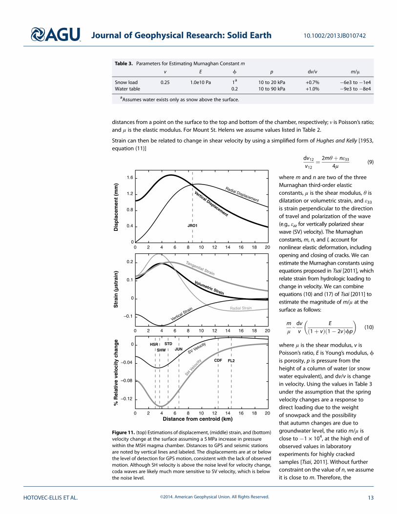
Figure 11. (top) Estimations of displacement, (middle) strain, and (bottom)velocity change at the surface assuming a 5MPa increase in pressurewithin the MSH magma chamber. Distances to GPS and seismic stationsare noted by vertical lines and labeled. The displacements are at or belowthe level of detection for GPS motion, consistent with the lack of observedmotion. Although SH velocity is above the noise level for velocity change,coda waves are likely much more sensitive to SV velocity, which is belowthe noise level.



maximum value of change in SV velocity for our theoretical magmatic intrusion is approximately �0.05%(Figure 11). Although strain and velocity increase with depth, this change is still near or below the level ofnoise with our method, so it is possible that a 5MPa pressure increase could have escaped detection evenwithout consideration of finite compressibility of a zone around the chamber [Mastin et al., 2008; Dzurisinet al., 2008]. Ueno et al. [2012] observed decreases in velocity of 0.2–0.8% during several intrusion-relatedswarms with estimated volumes on the order of a few thousand cubic meter; however, these intrusions werealso accompanied by measurable surface deformation and volumetric strain of more than 10�6. Ourpredicted strain is roughly an order of magnitude less than this, consistent with our lack of observablevelocity change. The choice of pressure increase is somewhat arbitrary but allows us to estimate an upperbound on the change in pressure in the chamber given our lack of detection to as much as 10MPa for achamber of 500m radius.

8. Conclusions

We used CWI to create a continuous record of seismic velocity change using triggered earthquake dataspanning nearly two decades to investigate the history of magma injection and pressurization of the MSHmagmatic system. This method is complementary to other studies of velocity change using continuous data,such as ambient noise interferometry, but can be applied to older data sets where continuous data areunavailable and only a triggered record exists. Temporal resolution of velocity change is dependent on therate of repeating seismicity and could also be applied to more frequent swarms of earthquakes, like thoseduring volcanic eruptions, to produce a record of velocity change on a significantly shorter timescale thanpresented here.

In this study, we did not resolve a velocity change due to magmatic intrusion(s), though the lack of velocitychange directly attributable to the volcano between the 1980–1986 and 2004–2008 eruptions is consistentwith a lack of precursory deformation. We concede that it is possible that intrusions occurred but did notpressurize the chamber enough to alter the shallow velocity structure to which this technique is mostsensitive. We estimate the maximum pressure change that could have escaped our detection to be on theorder of 10MPa, which is within the previously estimated bounds of pressure changes determined by deepearthquake focal mechanisms. We found well-resolved seismic velocity changes that are dominated byseasonal variability, likely caused by climatic forcing such as snow loading and shallow water tablefluctuations. In addition, the increased rate of seismicity is anticorrelated with the higher velocities in latewinter, and we believe this is most likely due to snow unloading. The most significant nonseasonal signal is adecrease in velocity at the time of the Nisqually earthquake, during which shaking dynamically likely caused apermanent alteration of the velocity structure. We suggest that the shallow seismicity and observed velocitychanges are indications that the volcano was pressurized and sensitive to relatively small pressure changes ofa few kilopascals well before the 2004 eruption.

ReferencesBattaglia, J., J. -P. Métaxian, and E. Garaebiti (2012), Earthquake-volcano interaction imaged by coda wave interferometry, Geophys. Res. Lett.,

39, L11309, doi:10.1029/2012GL052003.Bedrosian, P. A., M. Burgess, and A. Hotovec (2008), Groundwater hydrology within the crater of Mount St. Helens from geophysical

constraints, Eos Trans. AGU, 89(53), 2847 Fall Meet. Suppl., Abstract V43E-2191.Ben-Zion, Y., and P. Leary (1986), Thermoelastic strain in a half-space covered by unconsolidated material, Bull. Seismol. Soc. Am., 76,

1447–1460.Bonaccorso, A., and P. M. Davis (1999), Models of ground deformation from vertical volcanic conduits with application to eruptions of Mount

St. Helens and Mount Etna, J. Geophys. Res., 104(B5), 10,531–10,542.Brenguier, F., N. M. Shapiro, M. Campillo, V. Ferrazzini, Z. Duputel, O. Coutant, and A. Nercessian (2008a), Towards forecasting volcanic

eruptions using seismic noise, Nat. Geosci., 1, 126–130, doi:10.1038/ngeo104.Brenguier, F., M. Campillo, C. Hadziioannou, N. M. Shapiro, R. M. Nadeau, and E. Larose (2008b), Postseismic relaxation along the San Andreas

Fault at Parkfield from continuous seismological observations, Science, 321, 1478–1481, doi:10.1126/science.1160943.Carmona, E., J. Almendros, J. A. Peña, and J. M. Ibáñez (2010), Characterization of fracture systems using precise array locations of earthquake

multiplets: An example at Deception Island volcano, Antarctica, J. Geophys. Res., 115, B06309, doi:10.1029/2009JB006865.Christiansen, L. B., S. Hurwitz, M. O. Saar, S. E. Ingebritsen, and P. A. Hsieh (2005), Seasonal seismicity at western United States volcanic

centers, Earth Planet. Sci. Lett., 240, 307–321.Dodge, D. A., and G. C. Beroza (1997), Source array analysis of coda waves near the 1989 Loma Prieta, California, mainshock: Implications for

the mechanism of coseismic velocity changes, J. Geophys. Res., 102(B11), 24,437–24,458.Dzurisin, D., M. Lisowski, M. P. Poland, D. R. Sherrod, and R. G. LaHusen (2008), Constraints and conundrums resulting from ground-

deformation measurements made during the 2004-2005 dome-building eruption of Mount St. Helens, Washington, in A Volcano



AcknowledgmentsWaveform data and earthquake catalogused in this paper are courtesy of thePacific Northwest Seismic Network andare freely available upon request. Theauthors would like to thank Seth Moran,Weston Thelen, Stephanie Prejean,Steve Malone, and Matt Haney fordiscussions during preparation of thetext and Weston Thelen and FlorentBrenguier for their reviews.

http://dx.doi.org/10.1029/2012GL052003

http://dx.doi.org/10.1038/ngeo104

http://dx.doi.org/10.1126/science.1160943

http://dx.doi.org/10.1029/2009JB006865

Rekindled: The Renewed Eruption of Mount St. Helens, 2004–2006, edited by D. R. Sherrod, W. E. Scott, and P. H. Stauffer, Prof. Paper 1750,chap. 14, pp. 281–300, U.S. Geol. Surv., Reston, Va.

Gerlach, T. M., K. A. McGee, and M. P. Doukas (2008), Emission rates of CO2, SO2, and H2S, scrubbing, and preeruption excess volatiles atMount St. Helens, 2004–2005, in A Volcano Rekindled: The Renewed Eruption of Mount St. Helens, 2004–2006, edited by D. R. Sherrod,W. E. Scott, and P. H. Stauffer, Prof. Paper 1750, chap. 26, pp. 543–571, U.S. Geol. Surv., Reston, Va.

Grêt, A., R. Snieder, and J. Scales (2006), Time-lapse monitoring of rock properties with coda wave interferometry, J. Geophys. Res., 111,B03305, doi:10.1029/2004JB003354.

Hughes, D. S., and J. L. Kelly (1953), Second-order elastic deformation of solids, Phys. Rev., 92, 1145–1149.Hurwitz, S., K. L. Kipp, S. E. Ingebritsen, and M. E. Reid (2003), Groundwater flow, heat transport, and water table position within volcanic

edifices: Implications for volcanic processes in the Cascade Range, J. Geophys. Res., 108(B12), 2557, doi:10.1029/2003JB002565.Kanu, C. O., R. Snieder, and D. O’Connell (2013), Estimation of velocity change using repeating earthquakes with different locations and focal

mechanisms, J. Geophys. Res. Solid Earth, 118, 1–10, doi:10.1002/jgrb.50206.Lehto, H. L., D. C. Roman, and S. C. Moran (2013), Source mechanisms of persistent shallow earthquakes during eruptive and non-eruptive

periods between 1981 and 2011 at Mount St. Helens, Washington, J. Volcanol. Geotherm. Res., 256, 1–15, doi:10.1016/j.volgeores.2013.02.005.Li, Y.-G., P. Chen, E. S. Cochran, and J. E. Vidale (2007), Seismic velocity variations on the San Andreas fault caused by the 2004M6 Parkfield

Earthquake and their implications, Earth Planets Space, 59, 21–31.Lisowski, M. (2006) Analytical volcano deformation source models, in Volcano Deformation: Geodetic Monitoring Techniques, edited by

D. Dzurisin, chap. 8, pp. 279–304, Springer-Praxis, Chichester, U. K.Lisowski, M., D. Dzurisin, R. P. Denlinger, and E. Y. Iwatsubo (2008), Analysis of GPS-measured deformation associated with the 2004–2006

dome-building eruption of Mount St. Helens, Washington, in A Volcano Rekindled: The Renewed Eruption of Mount St. Helens, 2004–2006,edited by D. R. Sherrod, W. E. Scott, and P. H. Stauffer, Prof. Paper 1750, chap. 15, pp. 301–333, U.S. Geol. Surv., Reston, Va.

Massin, F., J. Farrell, and R. B. Smith (2013), Repeating earthquakes in the Yellowstone volcanic field: Implications for rupture dynamics,ground deformation, and migration in earthquake swarms, J. Volcanol. Geotherm. Res., 257, 159–173, doi:10.1016/j.jvolgeores.2013.03.22.

Mastin, L. G. (1994), Explosive tephra emissions at Mount St. Helens, 1989–1991: The violent escape of magmatic gas following storms?, Geol.Soc. Am. Bull., 106(2), 175–185.

Mastin, L. G., E. Roeloffs, N. M. Beeler, and J. E. Quick (2008), Constraints on the size, overpressure, and oolatile content of theMount St. Helensmagma system from geodetic and dome-growth measurements during the 2004–2006+ eruption, in A Volcano Rekindled: The RenewedEruption of Mount St. Helens, 2004–2006, edited by D. R. Sherrod, W. E. Scott, and P. H. Stauffer, Prof. Paper 1750, chap. 22, pp. 461–488,U.S. Geol. Surv., Reston, Va.

Meier, U., N. M. Shapiro, and F. Brenguier (2010), Detecting seasonal variations in seismic velocities within Los Angeles basin from correla-tions of ambient seismic noise, Geophys. J. Int., 181, 985–996.

Moran, S. C. (1994), Seismicity at Mount St. Helens, 1987–1992: Evidence for repressurization of an active magmatic system, J. Geophys. Res.,99(B3), 4341–4354.

Moran, S. C., S. D. Malone, A. I. Qamar, W. A. Thelen, A. K. Wright, and J. Caplan-Auerbach (2008), Seismicity associated with reneweddome building at Mount St. Helens, 2004–2005, in A Volcano Rekindled: The Renewed Eruption of Mount St. Helens, 2004–2006, editedby D. R. Sherrod, W. E. Scott, and P. H. Stauffer, Prof. Paper 1750, chap. 2, pp. 27–60, U.S. Geol. Surv., Reston, Va.

Musumeci, C., S. Gresta, and S. D. Malone (2002), Magma system recharge of Mount St. Helens from precise relative hypocenter location ofmicroearthquakes, J. Geophys. Res., 107(B10), 2264, doi:10.1029/2001JB000629.

Nakamura, A., A. Hasegawa, N. Hirata, T. Iwasaki, and H. Hamaguchi (2002), Temporal variations of seismic wave velocity associated with1998M6.1 Shizukuishi earthquake, Pure Appl. Geophys., 159, 1183–1204.

Pacheco, C., and R. Snieder (2005), Time-lapse travel time change of multiply scattered acoustic waves, J. Acoust. Soc. Am., 118(3), 1300–1310.Pallister, J. S., C. R. Thornber, K. V. Cashman, M. A. Clynne, H. A. Lowers, C. W. Mandeville, I. K. Brownfield, and G. P. Meeker (2008), Petrology of

the 2004–2006 Mount St. Helens lava dome—Implications for magmatic plumbing and eruption triggering, in A Volcano Rekindled:The Renewed Eruption of Mount St. Helens, 2004–2006, edited by D. R. Sherrod, W. E. Scott, and P. H. Stauffer, Prof. Paper 1750, chap. 30,pp. 648–702, U.S. Geol. Surv., Reston, Va.

Pandolfi, D., C. J. Bean, and G. Saccorotti (2006), Coda wave interferometric detection of seismic velocity changes associated with the 1999M = 3.6 event at Mt. Vesuvius, Geophys. Res. Lett., 33, L06306, doi:10.1029/2005GL025355.

Petersen, T. (2007), Swarms of repeating long-period earthquakes at Shishaldin Volcano, Alaska, 2001–2004, J. Volcanol. Geotherm. Res., 166,177–192, doi:10.1016/j.jvolgeores.2007.07.014.

Poland, M. P., and Z. Lu (2008), Radar interferometry observations of surface displacements during pre- and coeruptive periods at Mount St.Helens, Washington, 1992–2005, in A Volcano Rekindled: The Renewed Eruption of Mount St. Helens, 2004–2006, edited by D. R. Sherrod,W. E. Scott, and P. H. Stauffer, Prof. Paper 1750, chap. 18, pp. 361–382, U.S. Geol. Surv., Reston, Va.

Poupinet, G., W. L. Ellsworth, and J. Frechet (1984), Monitoring velocity variations in the crust using earthquake doublets: An application tothe Calaveras Fault, California, J. Geophys. Res., 89(B7), 5719–5731.

Ratdomopurbo, A., and G. Poupinet (1995), Monitoring a temporal change of seismic velocity in a volcano: Application to the 1992 eruptionof Mt. Merapi (Indonesia), Geophys. Res. Lett., 22(7), 775–778.

Rojstaczer, S., S. Wolf, and R. Michel (1995), Permeability enhancement in the shallow crust as a cause of earthquake-induced hydrologicalchanges, Nature, 373, 237–239.

Rubenstein, J. L., N. Uchida, and G. C. Beroza (2007), Seismic velocity reductions caused by the 2003 Tokachi-Oki earthquake, J. Geophys. Res.,112, B05315, doi:10.1029/2006JB004440.

Saccorotti, G., I. Lokmer, C. J. Bean, G. Di Grazia, and D. Patanè (2007), Analysis of sustained long-period activity at Etna Volcano, Italy,J. Volcanol. Geotherm. Res., 160, 340–354, doi:10.1016/.jvolgeores.2006.10.008.

Sawazaki, K., H. Sato, H. Nakahara, and T. Nishimura (2009), Time-lapse changes of seismic velocity in the shallow ground caused by strongground motion shock of the 2000 Western-Tottori earthquake, Japan, as revealed from coda deconvolution analysis, Bull. Seismol. Soc.Am., 99(1), 352–366, doi:10.1785/0120080058.

Scott, W. E., D. R. Sherrod, and C. A. Gardner (2008), Overview of the 2004 to 2006, and continuing, eruption of Mount St. Helens, Washington,in A Volcano Rekindled: The Renewed Eruption of Mount St. Helens, 2004–2006, edited by D. R. Sherrod, W. E. Scott, and P. H. Stauffer, Prof.Paper 1750, chap. 1, pp. 3–22, U.S. Geol. Surv., Reston, Va.

Sens-Schönfelder, C., and U. Wegler (2006), Passive image interferometry and seasonal variations of seismic velocities at Merapi Volcano,Indonesia, Geophys. Res. Lett., 33, L21302, doi:10.1029/2006GL027797.

Silver, P. G., T. M. Daley, F. Niu, and E. L. Majer (2007), Active source monitoring of cross-well seismic travel time for stress-induced changes,Bull. Seismol. Soc. Am., 97(1B), 281–293, doi:10.1785/0120060120.



http://dx.doi.org/10.1029/2004JB003354

http://dx.doi.org/10.1029/2003JB002565

http://dx.doi.org/10.1002/jgrb.50206

http://dx.doi.org/10.1016/j.volgeores.2013.02.005

http://dx.doi.org/10.1016/j.jvolgeores.2013.03.22

http://dx.doi.org/10.1029/2001JB000629

http://dx.doi.org/10.1029/2005GL025355

http://dx.doi.org/10.1016/j.jvolgeores.2007.07.014

http://dx.doi.org/10.1029/2006JB004440

http://dx.doi.org/10.1016/.jvolgeores.2006.10.008

http://dx.doi.org/10.1785/0120080058

http://dx.doi.org/10.1029/2006GL027797

http://dx.doi.org/10.1785/0120060120

Snieder, R. (2002), Coda wave interferometry and the equilibration of energy in elastic media, Phys. Rev. E, 66, 046615, doi:10.1103/PhysRevE.66.046615.

Snieder, R. (2006), The theory of coda wave interferometry, Pure Appl. Geophys., 163, 455–473, doi:10.1007/s00024-005-0026-6.Snieder, R., A. Grêt, H. Douma, and J. Scales (2002), Coda wave interferometry for estimating nonlinear behavior in seismic velocity, Science,

295, 2253–2255.Tatagi, R., T. Okada, H. Nakahara, N. Umino, and A. Hasegawa (2012), Coseismic velocity change in and around the focal region of the 2008

Iwate-Miyagi Nairiku earthquake, J. Geophys. Res., 117, B06315, doi:10.1029/2012JB009252.Thelen, W. A., R. S. Crosson, and K. C. Creager (2008), Absolute and relative locations of earthquakes at Mount St. Helens, Washington, using

continuous data: Implications for magmatic processes, in A Volcano Rekindled: The Renewed Eruption of Mount St. Helens, 2004–2006,edited by D. R. Sherrod, W. E. Scott, and P. H. Stauffer, Prof. Paper 1750, chap. 4, pp. 71–95, U.S. Geol. Surv., Reston, Va.

Thelen, W., S. Malone, and M. West (2011), Multiplets: Their behavior and utility at dacitic and andesitic volcanic centers, J. Geophys. Res., 116,B08210, doi:10.1029/2010JB007924.

Tsai, V. C. (2011), A model for seasonal changes in GPS positions and seismic wave speeds due to thermoelastic and hydrologic variations,J. Geophys. Res., 116, B04404, doi:10.1029/2010JB008156.

Ueno, T., T. Saito, K. Shiomi, B. Enescu, H. Hirose, and K. Obara (2012), Fractional seismic velocity change related to magma intrusions duringearthquake swarms in the eastern Izu peninsula, central Japan, J. Geophys. Res., 117, B12305, doi:10.1029/2012JB009580.

Wegler, U., B.-G. Lühr, R. Snieder, and A. Ratdomopurbo (2006), Increase of shear wave velocity before the 1998 eruption of Merapi volcano(Indonesia), Geophys. Res. Lett., 33, L09303, doi:10.1029/2006GL025928.

Wegler, U., H. Nakahara, C. Sens-Schönfelder, M. Korn, and K. Shiomi (2009), Sudden drop of seismic velocity after the 2004 Mw 6.6 mid-Niigata earthquake, Japan, observed with Passive Image Interferometry, J. Geophys. Res., 114, B06305, doi:10.1029/2008JB005869.

Yamada, M., J. Mori, and S. Ohmi (2010), Temporal changes of subsurface velocities during strong shaking as seen from seismic interfero-metry, J. Geophys. Res., 115, B03302, doi:10.1029/2009JB006567.



http://dx.doi.org/10.1103/PhysRevE.66.046615

http://dx.doi.org/10.1103/PhysRevE.66.046615

http://dx.doi.org/10.1007/s00024&hyphen;005&hyphen;0026&hyphen;6

http://dx.doi.org/10.1029/2012JB009252

http://dx.doi.org/10.1029/2010JB007924

http://dx.doi.org/10.1029/2010JB008156

http://dx.doi.org/10.1029/2012JB009580

http://dx.doi.org/10.1029/2006GL025928

http://dx.doi.org/10.1029/2008JB005869

http://dx.doi.org/10.1029/2009JB006567

publications - earth and space sciences at the university

Documents