OMAE 2004, Vancouver

Progress in wave load computations

on offshore structures

by J. N. Newmanjnn@mit.edu

Computational methods for predicting wave effects have obvious importance for the design and operation of offshore structures. The available tools range from simplified theories, and codes with restricted applications, to cutting-edge Navier-Stokes solvers which seek to account for all relevant viscous and nonlinear effects. It would be most valuable to survey this entire field, but given the restrictions of time and my own experience, I cannot do that in this lecture. Instead I will focus on the use of the panel method, sometimes known as the boundary integral equation method or boundary element method. This occupies a central position in the prediction of wave effects on large offshore structures, since it can be applied to a wide variety of practical applications, with sufficient confidence that it can be used by practitioners, not just by researchers. On the other hand we must keep in mind that panel methods are generally restricted by the assumptions of linear potential flow, although I will show some examples where we can take one or two steps beyond these strict limits.

3D linear computations1970-1980

• Panel methods (after Hess and Smith) Halkyard/Milgram, Garrison, Hogben/Standing, v.Oertmerssen, Faltinsen/Michelsen

• FEM Bai,Yue/Chen/Mei/Aranha, EatockTaylor/Wu

This list includes some of the pioneers on the computation of wave loads. The 3D panel method was first developed by Hess and Smith at the Douglas Aircraft Company. The name came from their representing the body surface by a large number of small flat quadrilateral `panels’. This approach was extended by several groups to include free surface effects. The early programs were very slow, and some attention was also given to finite-element methods where the entire fluid domain was discretized, but subsequent refinements of the panel method have largely superseded the FEM activity.

The TLP challenge1979-1991

• 2nd order (Molin, Lighthill, Kim/Yue)• Improved 1st order (linear) panel method

Fast Green function algorithms, iterative solvers (Korsmeyer et al, OMAE `88)

• 2nd-order codes (Chau/Eatock Taylor, Chen et al (BV), C-H Lee et al (MIT)

TLP's presented a number of challenges, regarding more efficient computation of linear solutions and the need to consider second-order nonlinearities. This led to many advances, so that by the early 1990's the use of panel methods was more universal and useful.

recent developments

• higher-order panel methods• exact geometry• CAD coupling• Accelerated solver O(N log N)• Viscous post-processor

Recent developments which I will discuss include higher-order panel methods, and more exact and convenient representations of the geometry. Also the development of accelerated solvers which are essential for extremely large complex structures, and coupled solutions of the potential and viscous problems.

Examples of Applications and Results

• Spar with strakes and moonpool• Drill ship with three moonpools• Damping of gap resonance between hulls• Linear coupling with internal tanks• VLFS (Mat structure and cylinder array)• Slowly-varying 2nd order drift force• Navier-Stokes post-processor (VISCOR)

Submerged surface of a spar with 3 strakes and a circular moonpool – draft 100m, radius 18m

Exact Geometryof submergedsurface

Low orderLow-orderN=264 panels(NEQN=264)

Higher-orderN=66 "panels"(NEQN=153)

This figure shows the submerged portion of a spar, consisting of a cylindrical hull with a concentric moonpool and 3 helical strakes. The left figure shows the exact geometry. The middle figure illustrates its representation in the low-order panel method, where the surface is approximated by quadrilateral flat panels and the solution for the potential or source strength is constant on each panel. The right-hand figure illustrates the higher-order method, where the surface is subdivided into eight `patches’, indicated here by different colors. The basic requirement is that the surface should be smooth and continuous on each separate patch. The geometry on each patch is mapped onto a rectangular parametric surface. In most practical applications this mapping is effectively exact, so there is no approximation of the geometry. The velocity potential is represented in each parametric space by continuous basis functions with unknown coefficients, and the solution for these coefficients is computed in a manner which is fundamentally similar to the low-order method. To control the accuracy of the solution, the parametric coordinates can be subdivided, as indicated by the black lines in the right figure. We use B-splines to represent the solution, and increasing the number of subdivisions is equivalent to adding knots and control points to the B-splines. The principal advantages of the higher-order method are that it gives a more accurate and efficient representation of the solution, and the only significant numerical approximation is in the solution itself, which can be controlled by increasing the number of subdivisions in the parametric space. This approach also circumvents the work of discretizing or panelling the body.

Surge exciting force on the sparDashed curves: low-order method with N panels

Solid curves: higher-order method with N unknowns

Period (seconds)10 15 20 25 300

500

1000

1500

2000

N=414N=1656N=6264N=162N=384N=1104

This figure shows the surge exciting force on the spar, plotted against the wave period. Results using both the low-order and higher-order methods are shown, with increasing numbers of unknowns to refine the accuracy. The convergence is apparent as the number of unknowns is increased, and the accuracy of both results can be judged by the extent to which they change with increasingly fine discretizations. Note that the accuracy of the coarsest higher-order discretization, with N=162, is comparable to the accuracy of the finest low-order discretization, with N=6264.

Yaw exciting moment on the spar Dashed curves: low-order method with N panels

Solid curves: higher-order method with N unknowns

Period (seconds)10 15 20 25 300

100

200

300

400

500

600

700 N=414N=1656N=6264N=162N=384N=1104

This figure shows the yaw moment, which is relatively small, since the strakes are the only surfaces which contribute. The singular feature near 20 seconds is due to the moonpool pumping mode resonance, which causes a large axisymmetric flux in and out of the moonpool. This has no noticeable effect on the surge force, but the induced exterior flow past the strakes produces a yaw moment.

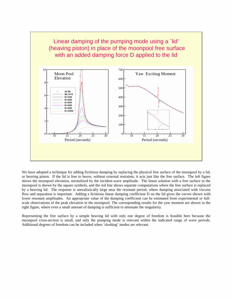
Linear damping of the pumping mode using a `lid’ (heaving piston) in place of the moonpool free surface

with an added damping force D applied to the lid

Period (seconds)10 15 20 25 300

100

200

300

400

500

600

700Yaw Exciting Moment

Period (seconds)10 15 20 25 300

2

4

6

8

10

no lidlid, D=0D=100D=200D=300D=400D=500D=1000

Moon PoolElevation

19 20 21340

360

380

400

420

We have adopted a technique for adding fictitious damping by replacing the physical free surface of the moonpool by a lid, or heaving piston. If the lid is free to heave, without external restraints, it acts just like the free surface. The left figure shows the moonpool elevation, normalized by the incident-wave amplitude. The linear solution with a free surface in the moonpool is shown by the square symbols, and the red line shows separate computations where the free surface is replaced by a heaving lid. The response is unrealistically large near the resonant period, where damping associated with viscous flow and separation is important. Adding a fictitious linear damping coefficient D on the lid gives the curves shown with lower resonant amplitudes. An appropriate value of the damping coefficient can be estimated from experimental or full-scale observations of the peak elevation in the moonpool. The corresponding results for the yaw moment are shown in the right figure, where even a small amount of damping is sufficient to attenuate the singularity. Representing the free surface by a simple heaving lid with only one degree of freedom is feasible here because the moonpool cross-section is small, and only the pumping mode is relevant within the indicated range of wave periods. Additional degrees of freedom can be included when `sloshing’ modes are relevant.

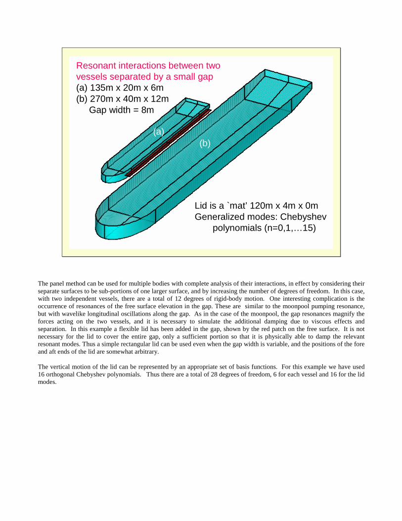
Resonant interactions between two vessels separated by a small gap(a) 135m x 20m x 6m(b) 270m x 40m x 12m

Gap width = 8m

Lid is a `mat’ 120m x 4m x 0mGeneralized modes: Chebyshev

polynomials (n=0,1,…15)

(b)(a)

The panel method can be used for multiple bodies with complete analysis of their interactions, in effect by considering their separate surfaces to be sub-portions of one larger surface, and by increasing the number of degrees of freedom. In this case, with two independent vessels, there are a total of 12 degrees of rigid-body motion. One interesting complication is the occurrence of resonances of the free surface elevation in the gap. These are similar to the moonpool pumping resonance, but with wavelike longitudinal oscillations along the gap. As in the case of the moonpool, the gap resonances magnify the forces acting on the two vessels, and it is necessary to simulate the additional damping due to viscous effects and separation. In this example a flexible lid has been added in the gap, shown by the red patch on the free surface. It is not necessary for the lid to cover the entire gap, only a sufficient portion so that it is physically able to damp the relevant resonant modes. Thus a simple rectangular lid can be used even when the gap width is variable, and the positions of the fore and aft ends of the lid are somewhat arbitrary. The vertical motion of the lid can be represented by an appropriate set of basis functions. For this example we have used 16 orthogonal Chebyshev polynomials. Thus there are a total of 28 degrees of freedom, 6 for each vessel and 16 for the lid modes.

Verification of method with Damping=0Lines: flexible mat -- Symbols: free surface

X

Ele

vatio

n

-60 -40 -20 0 20 40 600

1

2

3

4

5

6

Period=6.0Period=6.37Period=6.8Period=8.0Period=10.0

Here the use of the flexible lid is verified. The curves show the deflection of the lid, without damping, as a function of the longitudinal position X. The symbols show the more conventional computations of the free-surface elevation in the gap, without a lid. The computed results are practically identical. Five wave periods are shown, ranging from 6 to 10 seconds. The largest amplitude occurs at 6.37 seconds, represented by the red curve, with peak values about 5 times the incident-wave amplitude.

Effect of damping on lid deflectionPeriod=6.37 seconds

X

Ele

vatio

n

-60 -40 -20 0 20 40 600

1

2

3

4

5

6

D=0D=100D=200D=400D=1000

This shows the results for the peak period of the gap resonance, for a range of increasing damping coefficients. The elevations at the longer wave periods are not affected significantly.

Navis Explorer I with 3 moonpoolsGeometry definition from MultiSurf/RGKernel interface

(higher-order method)

In regard to the geometry, one can either describe this analytically, with appropriate equations, as was done for the two previous examples, or one can use a CAD program. In our paper two years ago at the Oslo OMAE I described in some detail how we have interfaced the CAD program MultiSurf with the higher-order solution in WAMIT, so that there is no need for an intermediate geometry file to be prepared by the user. That approach is illustrated here for a drillship which has 3 large moonpools.

Moonpool elevations compared to experiments Red curves are computations with damped lids

Black curves are experiments (MARINTEK) Hs=Significant Wave Height in meters

Period7 8 9 10 11 12 13 14 15 16

0

0.1

0.2

0.3

0.4

0.5

0.6

0.7

0.8

0.9

1

1.1

1.2Hs=5.0Hs=7.0Hs=16.9WAMIT

AFT MOONPOOL

Period7 8 9 10 11 12 13 14 15 16

0

0.1

0.2

0.3

0.4

0.5

0.6

0.7

0.8

0.9

1

1.1

1.2

FORWARD MOONPOOL

Period7 8 9 10 11 12 13 14 15 16

0

0.1

0.2

0.3

0.4

0.5

0.6

0.7

0.8

0.9

1

1.1

1.2

MIDDLE MOONPOOL

This shows the comparison between experimental data and computations for the moonpool elevations, with damped lids used for the computations. The elevations are normalized by the incident-wave amplitude. A single constant damping coefficient for the lids was selected to match the peaks. Three different sea states were used in the experiments, including the severe case with significant wave height 16.9m. Nonlinear effects are evident here, with smaller relative elevations in the highest sea state. Improved comparisons would probably result from the use of a stochastic linearization of the damping, so that larger lid damping coefficients are applied in the more severe sea states.

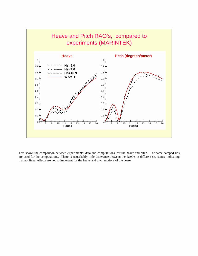
Heave and Pitch RAO’s, compared to experiments (MARINTEK)

Period7 8 9 10 11 12 13 14 15 16

0

0.1

0.2

0.3

0.4

0.5

0.6

0.7

0.8

0.9

1

Hs=5.0Hs=7.0Hs=16.9WAMIT

Heave

Period7 8 9 10 11 12 13 14 15 16

0

0.1

0.2

0.3

0.4

0.5

0.6

0.7

0.8

0.9

1

Pitch (degrees/meter)

This shows the comparison between experimental data and computations, for the heave and pitch. The same damped lids are used for the computations. There is remarkably little difference between the RAO's in different sea states, indicating that nonlinear effects are not so important for the heave and pitch motions of the vessel.

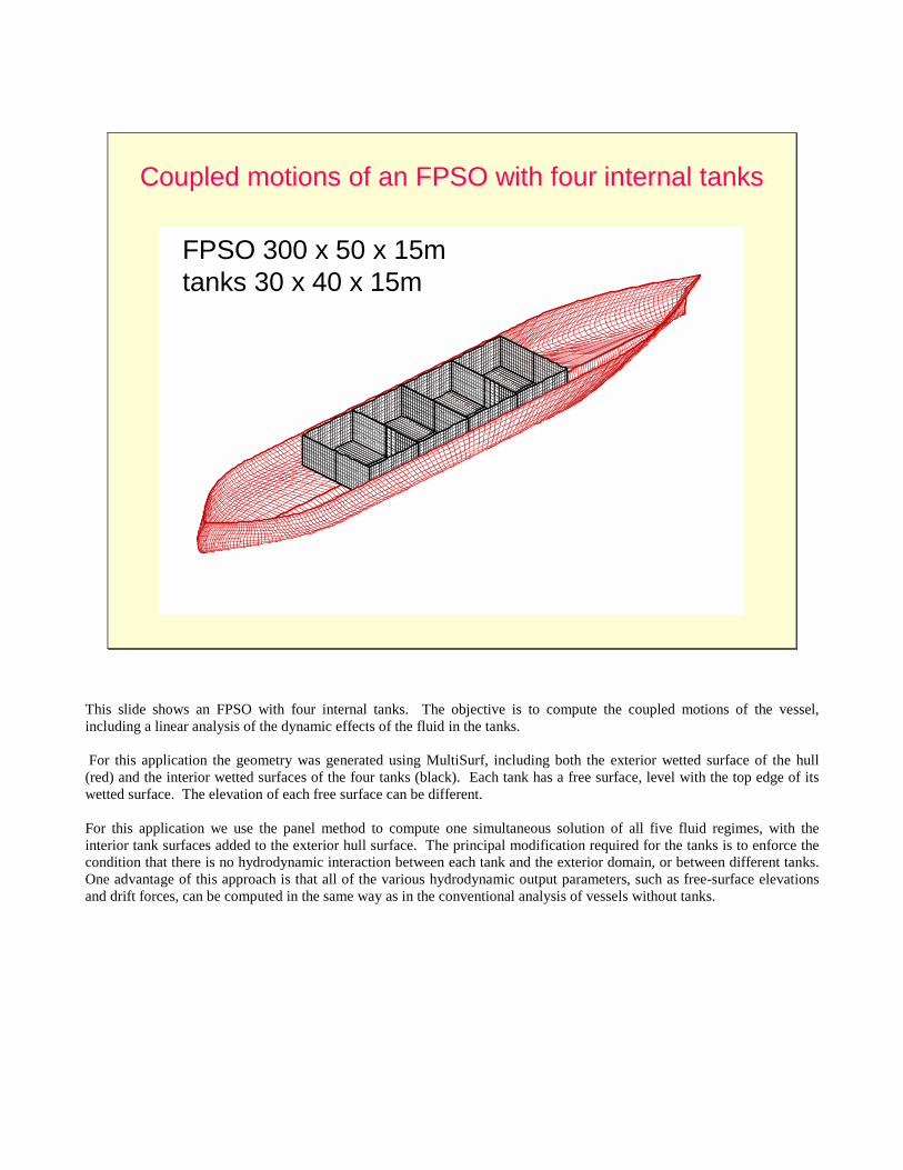
Coupled motions of an FPSO with four internal tanks

FPSO 300 x 50 x 15mtanks 30 x 40 x 15m

This slide shows an FPSO with four internal tanks. The objective is to compute the coupled motions of the vessel, including a linear analysis of the dynamic effects of the fluid in the tanks. For this application the geometry was generated using MultiSurf, including both the exterior wetted surface of the hull (red) and the interior wetted surfaces of the four tanks (black). Each tank has a free surface, level with the top edge of its wetted surface. The elevation of each free surface can be different. For this application we use the panel method to compute one simultaneous solution of all five fluid regimes, with the interior tank surfaces added to the exterior hull surface. The principal modification required for the tanks is to enforce the condition that there is no hydrodynamic interaction between each tank and the exterior domain, or between different tanks. One advantage of this approach is that all of the various hydrodynamic output parameters, such as free-surface elevations and drift forces, can be computed in the same way as in the conventional analysis of vessels without tanks.

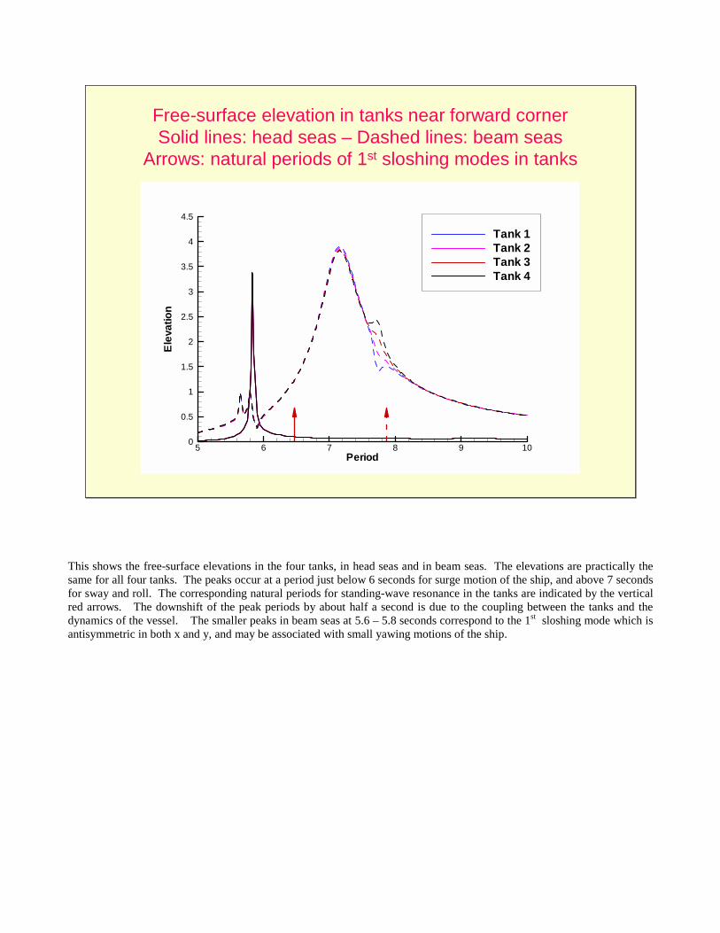
Free-surface elevation in tanks near forward cornerSolid lines: head seas – Dashed lines: beam seas

Arrows: natural periods of 1st sloshing modes in tanks

Period

Ele

vatio

n

5 6 7 8 9 100

0.5

1

1.5

2

2.5

3

3.5

4

4.5

Tank 1Tank 2Tank 3Tank 4

This shows the free-surface elevations in the four tanks, in head seas and in beam seas. The elevations are practically the same for all four tanks. The peaks occur at a period just below 6 seconds for surge motion of the ship, and above 7 seconds for sway and roll. The corresponding natural periods for standing-wave resonance in the tanks are indicated by the vertical red arrows. The downshift of the peak periods by about half a second is due to the coupling between the tanks and the dynamics of the vessel. The smaller peaks in beam seas at 5.6 – 5.8 seconds correspond to the 1st sloshing mode which is antisymmetric in both x and y, and may be associated with small yawing motions of the ship.

Sway/Roll RAO’s in beam seasrho = relative density of fluid in tanks

Period

Rol

lRA

O

5 6 7 8 9 10 11 12 13 14 150

0.2

0.4

0.6

0.8 rho=0rho=.5rho=.75rho=1

Period

Sw

ayR

AO

5 6 7 8 9 10 11 12 13 14 150

0.2

0.4

0.6

0.8

Here we see the sway and roll response of the FPSO in beam seas, for several different densities of the tank fluid. The total displacement is the same in all cases. The red curves, for zero density, are equivalent to the case where there are no tanks. Rapid variations occur near the sloshing resonance, and to account correctly for this regime it would be necessary to perform a nonlinear analysis of the tank dynamics, but even this linearized analysis demonstrates the strong influence of the tanks on the global response of the vessel.

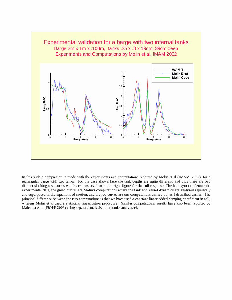
Experimental validation for a barge with two internal tanksBarge 3m x 1m x .108m, tanks .25 x .8 x 19cm, 39cm deepExperiments and Computations by Molin et al, IMAM 2002

Frequency

Sw

ayR

AO

2 4 6 8 100

0.5

1

Frequency

Rol

lRA

O

2 4 6 8 100

0.5

1

1.5

2

2.5

3

WAMITMolin ExptMolin Code

In this slide a comparison is made with the experiments and computations reported by Molin et al (IMAM, 2002), for a rectangular barge with two tanks. For the case shown here the tank depths are quite different, and thus there are two distinct sloshing resonances which are most evident in the right figure for the roll response. The blue symbols denote the experimental data, the green curves are Molin's computations where the tank and vessel dynamics are analysed separately and superposed in the equations of motion, and the red curves are our computations carried out as I described earlier. The principal difference between the two computations is that we have used a constant linear added damping coefficient in roll, whereas Molin et al used a statistical linearization procedure. Similar computational results have also been reported by Malenica et al (ISOPE 2003) using separate analysis of the tanks and vessel.

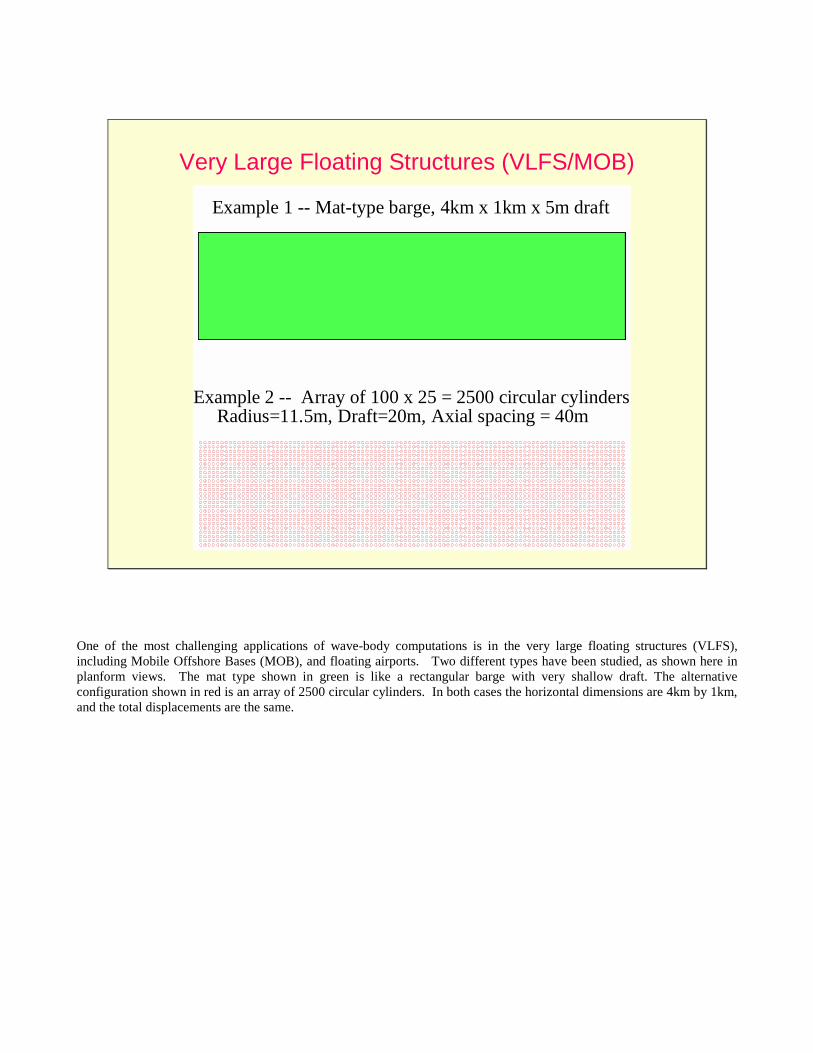
Very Large Floating Structures (VLFS/MOB)

Example 2 -- Array of 100 x 25 = 2500 circular cylindersRadius=11.5m, Draft=20m, Axial spacing = 40m

Example 1 -- Mat-type barge, 4km x 1km x 5m draft

One of the most challenging applications of wave-body computations is in the very large floating structures (VLFS), including Mobile Offshore Bases (MOB), and floating airports. Two different types have been studied, as shown here in planform views. The mat type shown in green is like a rectangular barge with very shallow draft. The alternative configuration shown in red is an array of 2500 circular cylinders. In both cases the horizontal dimensions are 4km by 1km, and the total displacements are the same.

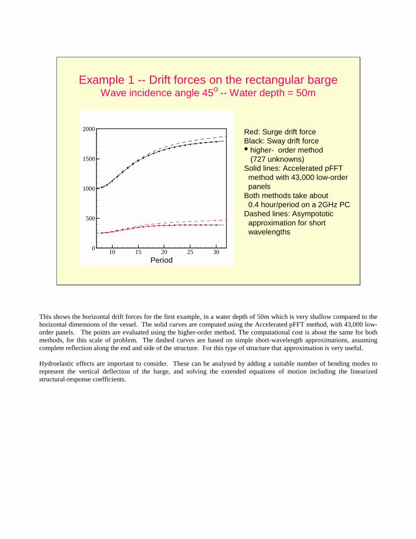
Example 1 -- Drift forces on the rectangular bargeWave incidence angle 45o -- Water depth = 50m

Red: Surge drift forceBlack: Sway drift force• higher- order method

(727 unknowns) Solid lines: Accelerated pFFT

method with 43,000 low-orderpanels

Both methods take about0.4 hour/period on a 2GHz PC

Dashed lines: Asympototicapproximation for shortwavelengths

Period10 15 20 25 300

500

1000

1500

2000

This shows the horizontal drift forces for the first example, in a water depth of 50m which is very shallow compared to the horizontal dimensions of the vessel. The solid curves are computed using the Accelerated pFFT method, with 43,000 low- order panels. The points are evaluated using the higher-order method. The computational cost is about the same for both methods, for this scale of problem. The dashed curves are based on simple short-wavelength approximations, assuming complete reflection along the end and side of the structure. For this type of structure that approximation is very useful. Hydroelastic effects are important to consider. These can be analysed by adding a suitable number of bending modes to represent the vertical deflection of the barge, and solving the extended equations of motion including the linearized structural-response coefficients.

Example 2 -- Drift forces on the 100x25 Cylinder ArrayWave incidence angle 45o -- Water depth = 50m

240,000 low-order panelswere used here (96 on eachcylinder).

These computations wereperformed on a 2.6GHz PC using the accelerated pFFTmethod (`precorrected FastFourier Transform’). TheCPU time averaged aboutone hour per period.

The peak magnitudes aremuch larger below 8 seconds,where near-trapping occursbetween adjacent cylinders.Period

10 15 20 25 30-20

0

20

40

60

80

100

120

140SurgeSway

This shows corresponding results for the array of 2500 cylinders, represented by 240,000 low-order panels. In this case the number of unknowns N is too large for the conventional approach, where the CPU time is proportional to N2 or N3. Instead we use the accelerated pFFT method, where the CPU time is proportional to (N log N). With this approach it is possible to solve problems of this complexity, even with a PC. There is obviously a strong variation due to constructive and destructive wave interactions among the elements of the array. At shorter wave periods below eight seconds near-trapping occurs, with larger oscillations.

2nd order slowly-varying drift force on FPSO

This application involves the slowly-varying drift force acting on an FPSO. To describe this phenomenon completely requires that we solve the second-order problem for the velocity potential. The complete solution is complicated by the fact that there is an inhomogeneous free surface boundary condition, corresponding to the forcing all over the free surface due to second-order wave interactions. Thus one must discretize not only the body surface, but also the free surface, over a very large computational domain. Further complicating this task is the fact that the computations must be repeated for all relevant combinations of the first-order wave frequencies and heading angles.

Slowly-varying 2nd order Sway Force on FPSO(including the complete 2nd order potential)

Period10 15 200

0.2

0.4

0.6

0.8

1

1.2 depth = infinite

Period10 15 200

0.2

0.4

0.6

0.8

1

1.2 depth = 100m

Period10 15 200

0.2

0.4

0.6

0.8

1

1.2 depth = 50m

Period10 15 200

1

2

3

4

5

6

7depth = 30m

00.050.10.150.2

δω

This shows the complete results, for the slowly-varying second-order sway force in beam seas. Four different depths are included since the effect of shallow water is especially important here. The plots show the amplitudes of the quadratic transfer functions, including only the difference-frequency components which contribute to low-frequency forcing. The horizontal scales are the mean wave periods, which are derived from the mean frequencies of the two incident wave components. The colored lines correspond to different values of the difference between the two frequencies, as shown in the legend on the right. The black curves are for zero difference-frequency, equivalent to the mean drift force in monochromatic waves. Note that the vertical scale is changed in the first plot, for a depth of 30m, and the slowly-varying forces in this case are much larger for wave periods above 10 seconds. In the analysis of slowly-varying drift motions it is common to approximate the magnitudes of the quadratic transfer functions by the steady drift forces at the same mean frequencies. This greatly simplifies the analysis of low-frequency motions. This is relatively useful in deep water, as indicated by the close agreement between the black and red curves in the lower plots. However, as the depth is decreased below 100m, this approximation is poor. .

Slowly-varying 2nd order Sway Force on FPSOSolid lines – complete, Dashed lines -- approximate

Period10 15 200

1

2

3

4

5

6

7 depth = 30m

Period10 15 200

0.2

0.4

0.6

0.8

1

1.2 depth = 100m

Period10 15 200

0.2

0.4

0.6

0.8

1

1.2 depth = infinite

Period10 15 200

0.2

0.4

0.6

0.8

1

1.2 depth = 50m

00.050.10.150.2

δω

Fortunately, the most important component of the second-order potential in shallow water is associated with the incident waves, as shown here. The solid lines are the complete solution as in the previous slide. The dashed curves include the effects of the second-order incident wave potential, and its diffraction by the vessel, but not the more complicated potential resulting from the second-order forcing on the free surface. This gives much better results in shallow water, compared to the approximation based on the steady drift forces.

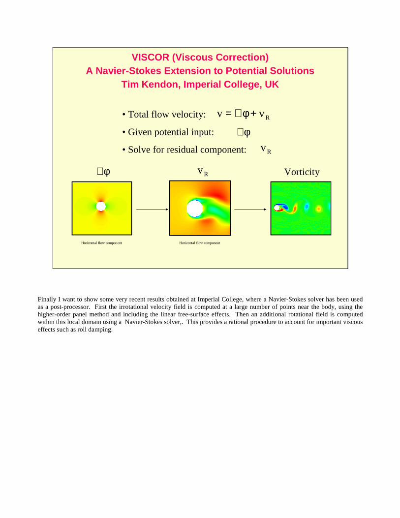
VISCOR (Viscous Correction)A Navier-Stokes Extension to Potential Solutions

Tim Kendon, Imperial College, UK

• Total flow velocity:

• Given potential input:

• Solve for residual component:

Rvv +φ∇=

φ∇

Vorticityφ∇

Rv

Rv

Horizontal flow componentHorizontal flow component

Finally I want to show some very recent results obtained at Imperial College, where a Navier-Stokes solver has been used as a post-processor. First the irrotational velocity field is computed at a large number of points near the body, using the higher-order panel method and including the linear free-surface effects. Then an additional rotational field is computed within this local domain using a Navier-Stokes solver,. This provides a rational procedure to account for important viscous effects such as roll damping.

This is a cross-section of a rolling rectangular barge, showing the computational domain for the rotational flow and concentrated regions of shed vorticity.

Moments in plane for B/T=2, freq = 0.67Hz

At a more quantitative level, this slide shows the time history of the roll moment, which attains its extreme values practically in phase with the maxima of the roll velocity. The roll moment is almost entirely due to the normal pressure, as opposed to the shear stress.

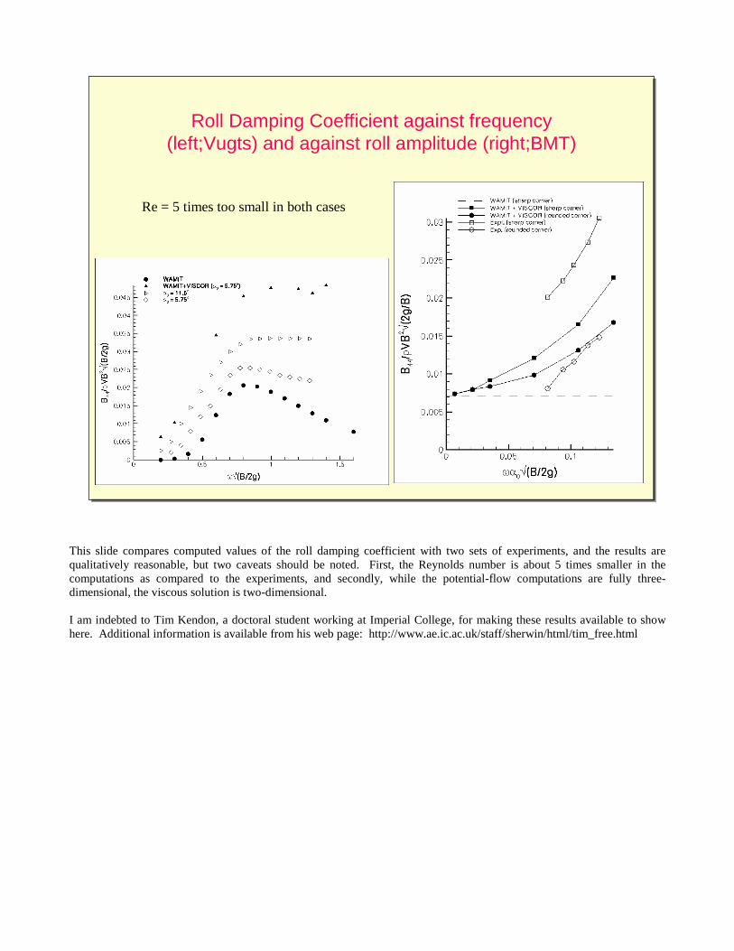
This slide compares computed values of the roll damping coefficient with two sets of experiments, and the results are qualitatively reasonable, but two caveats should be noted. First, the Reynolds number is about 5 times smaller in the computations as compared to the experiments, and secondly, while the potential-flow computations are fully three-dimensional, the viscous solution is two-dimensional. I am indebted to Tim Kendon, a doctoral student working at Imperial College, for making these results available to show here. Additional information is available from his web page: http://www.ae.ic.ac.uk/staff/sherwin/html/tim_free.html

Roll Damping Coefficient against frequency (left;Vugts) and against roll amplitude (right;BMT)

Re = 5 times too small in both cases

Roll Damping Coefficient against frequency (left;Vugts) and against roll amplitude (right;BMT)

Re = 5 times too small in both cases

Conclusions

• There has been tremendous progress in the computation of wave loads (in ~40 years!)

• Advances in (a) theoretical methods, (b) computational resources (hardware), and (c) computational methods (software)

• Big challenges remain (nonlinear and viscous effects, complex structures, unique applications)

Further information:

• www.wamit.com � Publications

• “Computation of wave effects using the panel method,” by C.-H. Lee and J. N. Newman, to be published in Numerical Modeling in Fluid-Structure Interaction, Edited by Subrata Chakrabarti, WIT Press, 2004