extreme wave loading on offshore wave energy devices using cfd
TRANSCRIPT

Extreme Wave Loading on Offshore Wave
Energy Devices using CFD
Jan Westphalen
University of Plymouth
A thesis submitted to the University of Plymouth in partial fulfilment of the
requirements for the degree of
Doctor of Philosophy
June 20, 2011

Abstract
Two commercial Navier-Stokes solvers are applied to wave-wave and wave-structure
interaction problems leading to the final application of simulating a single float of
the wave energy converter (WEC) Manchester Bobber in extreme waves and a fixed
section of the Pelamis in regular waves.
First the two software packages CFX and STAR CCM+ are validated against
measured results from physical tank tests concerning the interaction of 3 non-linear
focused wave groups of different steepness (Ning et al. 2007). The agreement for
all of these cases is very good and could even be improved from first order to second
order wave setup at the wavemaker. However, in preliminary regular wave tests, the
damping of the waves is identified to be an issue, which is the reason for focusing
the waves and placing the structures in the following experiments approximately
one wavelength behind the wavemaker.
The interaction of fixed vertical and horizontal cylinders in regular waves are
simulated concerning the forces on the structures (Kriebel 1998, Dixon et al. 1979).
For the horizontal cylinder non-linear force oscillations of double the wave fre-
quency could be modelled in good agreement with physical tank data, where lin-
earised models failed. For the vertical cylinder the problem of the secondary load
cycle due to a backward-breaking wave behind the cylinder is of special interest
(Stansberg 1997, Chaplin et al. 1997). Here, the horizontal forces on a slender
cylinder with a diameter approximately equal to the wave height are simulated suc-
cessfully. Furthermore, the highly non-linear wave run-up in front of the cylinder is
resolved well in the numerical approach.
The next set of simulations includes rigid body motion. Here, the forced oscil-
lations of a cone shaped body near the still water surface is simulated. These results
are compared with test data published by Drake et al. (2008). For these cases the
non-linearity of the experiments is discussed by comparing the sum and differences
of the force and surface elevation time histories for a set of simulations with op-
posite excursion of the cone. The hydrodynamic forces on the cone surface are
resolved in very good agreement. The solution of the surface elevation close to the
iii

cone surface is also resolved reasonably well.
After having validated the codes for fixed wave-structure interaction problems
and forced motion, the CFD methods are finally applied to problems relevant to the
survivability of WECs. First a single float in waves is modelled. This challenging
case combines the extreme wave setup with a floating body problem in one and two
degrees of freedom including the interaction of the float inertia with the inertia of
a separate mass attached to it. The vertical translations of the float are compared
with physical tank tests by Stallard et al. (2008). This case clearly demonstrates the
capabilities and challenges in using CFD to simulate WECs. When representing the
pulley and counterweight system by a simplified external body force rather than the
full setup, the calculated translations of the float agreed better with the measured
results from the physical tank test.
Furthermore the codes are used to simulate a single fixed section of the Pelamis
device in regular waves. The surface elevations close to the device are discussed
and the forces acting on different strips on the structure are presented.
iv

Contents
Abstract iv
Acknowledgements xi
Author’s declaration xiii
1 Introduction 1
2 Literature Review 5
3 Mathematical Models 34
3.1 Governing Equations . . . . . . . . . . . . . . . . . . . . . . . . . 34
3.2 Solution of the Governing Equations . . . . . . . . . . . . . . . . . 43
3.2.1 Discretisation of NSE . . . . . . . . . . . . . . . . . . . . 43
3.2.2 Pressure-Velocity Coupling . . . . . . . . . . . . . . . . . 50
3.2.3 Gradient Computation . . . . . . . . . . . . . . . . . . . . 51
3.2.4 Boundary Conditions . . . . . . . . . . . . . . . . . . . . . 56
3.2.5 Interface Capturing . . . . . . . . . . . . . . . . . . . . . . 60
3.2.6 Solution Methods . . . . . . . . . . . . . . . . . . . . . . . 64
4 Wave-Wave Interaction 70
4.1 Regular Waves . . . . . . . . . . . . . . . . . . . . . . . . . . . . 70
4.1.1 Computational Domain for Regular Waves . . . . . . . . . 70
4.1.2 Generation of Regular Waves . . . . . . . . . . . . . . . . 71
4.1.3 Grid Convergence Study . . . . . . . . . . . . . . . . . . . 72
4.1.4 Damping of Waveheight in the Numerical Wave Tank . . . . 74
4.2 Focused Waves . . . . . . . . . . . . . . . . . . . . . . . . . . . . 74
4.2.1 Domain for Focused Waves . . . . . . . . . . . . . . . . . 77
4.2.2 Generation of Focused Waves . . . . . . . . . . . . . . . . 80
4.2.3 Implementation of Boundary Conditions . . . . . . . . . . 85
v

4.2.4 Focused wave results . . . . . . . . . . . . . . . . . . . . . 88
4.2.5 Non-linearity of Focused Waves . . . . . . . . . . . . . . . 91
5 Wave-Structure Interaction 101
5.1 Vertical Cylinder . . . . . . . . . . . . . . . . . . . . . . . . . . . 101
5.1.1 Computational Domain . . . . . . . . . . . . . . . . . . . . 102
5.1.2 Results of vertical cylinder case . . . . . . . . . . . . . . . 105
5.1.3 Slender vertical cylinder and ringing of cylinder . . . . . . . 108
5.2 Horizontal Cylinder . . . . . . . . . . . . . . . . . . . . . . . . . . 111
5.2.1 Computational Domain and Meshes . . . . . . . . . . . . . 116
5.2.2 Results of horizontal cylinder case . . . . . . . . . . . . . . 117
5.3 Oscillating Cone . . . . . . . . . . . . . . . . . . . . . . . . . . . 123
5.3.1 Motion of the cone . . . . . . . . . . . . . . . . . . . . . . 125
5.3.2 Computational Domain and Meshes . . . . . . . . . . . . . 125
5.3.3 Oscillating Cone Results . . . . . . . . . . . . . . . . . . . 127
6 Simulation of WECs 143
6.1 Manchester Bobber . . . . . . . . . . . . . . . . . . . . . . . . . . 143
6.1.1 Single float in focused waves . . . . . . . . . . . . . . . . . 145
6.1.2 Reproduction of wave signal from physical tank tests . . . . 148
6.1.3 Computational Domain and Meshes . . . . . . . . . . . . . 151
6.1.4 Hydrodynamics of bobbing float . . . . . . . . . . . . . . . 156
6.1.5 Numerical performance . . . . . . . . . . . . . . . . . . . 168
6.2 Pelamis . . . . . . . . . . . . . . . . . . . . . . . . . . . . . . . . 171
6.2.1 Description of the Device . . . . . . . . . . . . . . . . . . 171
6.2.2 Simulation of a fixed single section in regular waves . . . . 172
6.2.3 Wave Loads on the Section . . . . . . . . . . . . . . . . . . 173
7 Conclusions 188
Nomenclature 199
Index. 204
List of references. 206
vi

A Java Macro used for the FV solver 217
B Fortran Routine used for the CV-FE solver 222
Bound copies of published papers. 242
vii

List of Figures
3.1 Fluid element . . . . . . . . . . . . . . . . . . . . . . . . . . . . . 35
3.2 CV arrangement . . . . . . . . . . . . . . . . . . . . . . . . . . . . 44
3.3 Surface element normal vector . . . . . . . . . . . . . . . . . . . . 47
3.4 Cell-centred discretisation scheme . . . . . . . . . . . . . . . . . . 48
3.5 Vertex-centred discretisation . . . . . . . . . . . . . . . . . . . . . 49
3.6 CV-FE shape function . . . . . . . . . . . . . . . . . . . . . . . . . 54
3.7 Boundary control volume for vertex-centred mesh arrangement . . . 58
3.8 Normalised Variable Diagramm . . . . . . . . . . . . . . . . . . . 61
3.9 CICSAM scheme . . . . . . . . . . . . . . . . . . . . . . . . . . . 62
3.10 Solution strategy for the coupled solver (ANSYS 2006) . . . . . . . 65
4.1 Regular wave domain . . . . . . . . . . . . . . . . . . . . . . . . . 71
4.2 Mesh section of STAR CCM+ meshes . . . . . . . . . . . . . . . . 73
4.3 Mesh section of CFX 5.7 meshes . . . . . . . . . . . . . . . . . . . 74
4.4 Surface elevation at x = 10m . . . . . . . . . . . . . . . . . . . . . 75
4.5 Damping in the NWT . . . . . . . . . . . . . . . . . . . . . . . . . 76
4.6 Computational domain . . . . . . . . . . . . . . . . . . . . . . . . 78
4.7 Input spectra for generation of focused wave group . . . . . . . . . 81
4.8 User scripting in STAR CCM+ and CFX . . . . . . . . . . . . . . . 88
4.9 Surface elevation at focus point for kA = 0.2 (Case 2) . . . . . . . . 90
4.10 Surface elevation at focus point for kA = 0.3 (Case 3) . . . . . . . . 92
4.11 Surface elevation at focus point for kA = 0.405 (Case 4) . . . . . . . 93
4.12 Sum and difference plots for the CV-FE solver (CFX) . . . . . . . . 94
4.13 Spectra from difference and sum plots (kA = 0.2, Case 2) . . . . . . 97
4.14 Filtered difference and sum results (kA = 0.2, Case 2) . . . . . . . . 98
4.15 Spectra from difference and sum plots (kA = 0.405, Case 4) . . . . . 99
4.16 Filtered difference and sum results (kA = 0.405, Case 4) . . . . . . . 100
5.1 Numerical wavetank for vertical cylinder . . . . . . . . . . . . . . . 103
viii

5.2 Mesh around large vertical cylinder . . . . . . . . . . . . . . . . . 104
5.3 Mesh refinement for both codes . . . . . . . . . . . . . . . . . . . 106
5.4 Horizontal forces on large vertical cylinder for both wave environ-
ments . . . . . . . . . . . . . . . . . . . . . . . . . . . . . . . . . 107
5.5 Secondary load cycle . . . . . . . . . . . . . . . . . . . . . . . . . 108
5.6 Surface elevation around slender cylinder . . . . . . . . . . . . . . 110
5.7 Surface elevation around slender cylinder . . . . . . . . . . . . . . 112
5.8 Surface elevation around slender cylinder . . . . . . . . . . . . . . 113
5.9 Surface elevation around slender cylinder . . . . . . . . . . . . . . 114
5.10 Surface elevation around slender cylinder . . . . . . . . . . . . . . 115
5.11 Domain of horizontal cylinder calculations . . . . . . . . . . . . . . 117
5.12 Horizontal cylinder meshes . . . . . . . . . . . . . . . . . . . . . . 118
5.13 Vertical forces on horizontal cylinder (d = 0.0 m) . . . . . . . . . . 120
5.14 Vertical forces on horizontal cylinder (d = -0.075 m) . . . . . . . . 120
5.15 Vertical forces on horizontal cylinder (d = -0.15 m) . . . . . . . . . 121
5.16 Surface elevation around cylinder (d = 0.0 m) . . . . . . . . . . . . 121
5.17 Surface elevation around cylinder (d = -0.15 m) . . . . . . . . . . . 122
5.18 Relative vertical force on cylinder, 2d vs 3d . . . . . . . . . . . . . 124
5.19 Computational domain for oscillating cone case . . . . . . . . . . . 126
5.20 Forces on cone for m=3 . . . . . . . . . . . . . . . . . . . . . . . . 130
5.21 Forces on cone for m=7 . . . . . . . . . . . . . . . . . . . . . . . . 131
5.22 Forces on cone for m=9 . . . . . . . . . . . . . . . . . . . . . . . . 132
5.23 Surface elevation around cone (m=3) . . . . . . . . . . . . . . . . . 133
5.24 Surface elevation around cone (m=7) . . . . . . . . . . . . . . . . . 134
5.25 Surface elevation around cone (m=9) . . . . . . . . . . . . . . . . . 135
5.26 Jet formation around cone (m = 9) . . . . . . . . . . . . . . . . . . 136
5.27 A = +/-0.05 m; Sum and difference of surface elevation (m = 3) . . . 137
5.28 A = +/-0.05 m; Sum and difference of surface elevation (m = 7) . . . 138
5.29 A = +/-0.05 m; Sum and difference of surface elevation (m = 9) . . . 139
5.30 Force components for m=3 . . . . . . . . . . . . . . . . . . . . . . 140
5.31 Force components for m=7 . . . . . . . . . . . . . . . . . . . . . . 141
5.32 Force components for m=9 . . . . . . . . . . . . . . . . . . . . . . 142
ix

6.1 Artists impression of The Manchester Bobber . . . . . . . . . . . . 144
6.2 Array of Floats in 70th scale (http://www.machesterbobber.com) . . 145
6.3 Geometry of a single float with counterweight and drive train . . . . 146
6.4 Free body diagramm of single float with counterweight . . . . . . . 147
6.5 Input spectra for generation of focused wave group . . . . . . . . . 150
6.6 Calculated surface elevations at focus point without float and 1st
and 2nd order wave signal (FV) . . . . . . . . . . . . . . . . . . . 151
6.7 Domain for single float simulations . . . . . . . . . . . . . . . . . . 152
6.8 Mesh around float . . . . . . . . . . . . . . . . . . . . . . . . . . . 153
6.9 Representation of mechanical system in CFD package through body
forces . . . . . . . . . . . . . . . . . . . . . . . . . . . . . . . . . 157
6.10 Vertical translation of float for tethered cases A and B . . . . . . . . 158
6.11 Vertical and horizontal forces on bobber float in extreme waves
(Cases A and B) . . . . . . . . . . . . . . . . . . . . . . . . . . . . 160
6.12 Single untethered float in physical experiment (Stallard 2010) . . . . 163
6.13 Single untethered float in physical experiment (Stallard 2010) . . . . 164
6.14 Hydrodynamics of untethered float (Case C) . . . . . . . . . . . . . 167
6.15 Vertical translation of float (Cases D1 and D2) . . . . . . . . . . . . 169
6.16 Vertical translation of float (Case E) . . . . . . . . . . . . . . . . . 169
6.17 Elapsed time vs. float velocity . . . . . . . . . . . . . . . . . . . . 170
6.18 Domain for single Pelamis section simulations . . . . . . . . . . . . 173
6.19 Mesh sections near structure . . . . . . . . . . . . . . . . . . . . . 174
6.20 Total force on single Pelamis section . . . . . . . . . . . . . . . . . 178
6.21 Side view on Pelamis section in regular waves (CFX) . . . . . . . . 179
6.22 Side view on Pelamis section in regular waves (STAR CCM+) . . . 180
6.23 Heave and drift forces calculated by CV-FE solver (CFX) . . . . . . 181
6.24 Heave and drift forces calculated by FV solver (STAR CCM+) . . . 182
6.25 View from top on Pelamis section in regular waves (CFX) . . . . . 185
6.26 View from top on Pelamis section in regular waves (STAR CCM+) . 186
6.27 Mesh around single section (view from above) . . . . . . . . . . . . 187
x

Acknowledgements
On this page I would like to thank all those people, who were involved during the
process of writing this thesis, running and setting up the simulations and interpreting
the results.
First of all I would like to thank Deborah for her help and advice during the
last 3 1/2 years, for reading through my “German” English over and over again
and giving me the opportunity to attend all the different conferences. I genuinely
enjoyed the last couple of years, first in Bath and then in Plymouth.
Alison and Chris I would like to thank for adding additional expertise and opin-
ions on this subject, which often put the problems into another perspective. Also,
the proofreading of my paper drafts and thesis chapters was incredible helpful.
The people involved in the project contributed to this work by asking a lot of
questions and commenting on my presentations and paper drafts during our project
meetings in Bath, Oxford and Manchester. A big “Thank you” to Paul Taylor, Derek
Causon, Peter Stansby, Zheng Zheng Hu and Pourya Omidvar. Many thanks to Jun
Zang, Kevin Drake and Tim Stallard for providing the experimental test data that
we used for our comparisons with the CFD codes.
Andrew Sunderland from HPCx also put in an awful lot of work for getting the
two packages to run on the cluster. Thanks to the ANSYS and CD-Adapco support
teams, for answering my questions so quickly.
Finally, this work was funded by the Engineering and Physical Science Research
Council under the project title “Extreme Wave Loading on Offshore Wave Energy
Devices using CFD: a Hierarchical Team Approach”. Thanks for that!
xi

Authors declaration
At no time during the registration for the degree of Doctor of Philosophy has the
author been registered for any other University award.
Relevant scientific seminars and conferences were regularly attended at which
work was often presented. One papers have been submitted for publication in Ocean
Engineering.
Signed:
Date:
Publications :
Westphalen, J., Greaves, D.M., Williams, C.J.K., Hunt-Raby, A.C.& Zang,
J. Focused waves and wave-structure interaction in a numerical wave tank.
submitted for publication in Ocean Engineering. 2010
Conference presentations :
2010:
The 20th International Offshore (Ocean) and Polar Engineering Conference
& Exibition, 20–26 June, Beijing, China. Oral presentation: Numerical Sim-
ulation of Wave Energy Converters using Eulerian and Lagrangian CFD
Methods .
Marine & Offshore Renewable Energy, 21–23 April, London, UK. Oral pre-
sentation: Numerical simulation of a floating body in multiple degrees of
freedom .
2009:
European Wave and Tidal Energy Conference, 7–10 September, Uppsala,
Sweden. Oral presentation: Extreme Wave Loading on Offshore Wave En-
ergy Devices using CFD: a Hierarchical Team Approach .
xii

24th International Workshop on Water Waves and Floating Bodies, 19–22
April, St. Petersburg, Russia. Oral presentation: Numerical Simulation of
an Oscillating Cone at the Water Surface using Computational Fluid Dy-
namics .
2008:
The 18th International Offshore (Ocean) and Polar Engineering Conference
& Exibition, 6–11 July, Vancouver, Canada. Oral presentation: Numerical
Simulation of Extreme Free Surface Waves.
2007:
Understanding Marine Systems, 17th December, Plymouth, UK. Oral presen-
tation: Extreme Wave Loading on Offshore Wave Energy Devices using
CFD.
10th Numerical Towing Tank Symposium, 23–25 September, Hamburg, Ger-
many. Oral presentation: Comparison of Free Surface Wave Simulations
using STAR CCM+ and CFX .
Word count for the main body of this thesis : 41,000
xiii

Chapter 1
Introduction
Modern western life style is heavily dependent on the growth of industrial produc-
tion, mobility and telecommunication, all of which rely on the supply of energy or
electricity. If either of these should break down, it would have a tremendous effect
on our life. People might not be able to commute to work, food supply might come
to a still stand or the telephone and internet networks would fail, which would effect
all kinds of areas immediately. Thus it is essential to secure the supply of energy
and meet the demand. On the other hand the customers need to be able to afford this
electricity. For example private people need to heat and light their houses, or simply
want to run their TV or kitchen appliances. These two requirements of the energy
sector, i.e. security of supply and the affordability of the energy are opposed by the
necessity of producing electricity in a environmentally friendly way. This includes
the reduction of CO2 emissions generated by burning fossil fuels, such as coal, oil
and gas, and the reduction of radioactive waste from nuclear power plants. Both of
these methods of generating electricity would be cheap and meet the demand. How-
ever, fossils are running out at some point in the future and nuclear waste pollutes
the environment for a very long time. Facing this trilemma of meeting the demand
at a low cost and in an environmentally friendly way is the challenge the energy sup-
pliers face today, which is the reason for developing alternative technologies, such
as wind energy, solar or hydro power, to substitute the traditional energy production
1

methods.
The hydro energy sector includes onshore energy production, such as river or
storage power stations, and coastal and offshore energy production, which can be
utilising tidal stream power, offshore wind and wave energy. As the onshore hydro
power production is almost saturated, the offshore sector is being developed heavily.
Here, the first option was to use established technologies, such as wind turbines, and
put them offshore. This was followed by tidal energy devices, which were adapted
from river power stations. Over the last 30 years the development of wave energy
devices caught up and is a quickly growing market with a variety of designs for
wave energy converters (WEC). However, this new technology is still expensive
compared to the traditional methods of generating electricity, but does not pollute
the environment and has the potential to meet the demand due to the shear size of
the oceans.
To be competitive the production costs of electricity by WECs need to be re-
duced. This can be achieved by putting a large number of wave energy converters
into place, make each of them more efficient during normal operation and reduce
maintenance costs, which is a key factor in offshore engineering in general. Re-
search is being done on the efficiency of devices using physical tank tests and
linearised numerical models, in which the waves are relatively small. This work,
however, looks into the latter design requirement by investigating the survivabil-
ity of WECs. In normal sea states this is not an issue, but when storm seas arise,
the WEC may be hit by very large waves, which might damage or even destroy
the device. Traditionally, this phenomenon is investigated using scale model tank
tests and linearised mathematical approaches, which might neglect rigid body mo-
tion or may not be able to simulate breaking waves. Relevant literature is discussed
2

in Chapter 2. Computational fluid dynamics (CFD) can provide an additional tool
when investigating such problems, that can model fluid-structure interaction includ-
ing wave-breaking, over topping and rigid body motion in a fully non-linear manner
and in full scale.
For this work two commercial CFD packages are applied to wave-wave and
wave-structure interaction problems relevant for the simulation of WECs. They both
solve the Navier-Stokes equations and model both fluids, water and air. The gov-
erning equations leading to the Navier-Stokes equations, the descretisation schemes
used for the solvers and the solution methodologies are described in Chapter 3.2.
First wave-only cases are simulated, which are described in Chapter 4. Here, the
implementation of the boundary conditions for the numerical models are described.
Results for regular and focused wave simulations are discussed and compared with
physical tank tests.
After that, fixed vertical and horizontal cylinders are modelled and the results are
compared with physical test data from the literature in Chapter 5. These simulations
concern the forces on the structures due to the waves. Non-linear effects such as the
ringing on slender vertical cylinder are identified and reproduced in the simulations.
This section finishes with the case of a cone, that is forced to move near the water
surface following a prescribed displacement. Here, the hydrodynamic forces and
the surface elevation close to the structure are compared with physical tank tests.
The final Chapter 6 discusses the application of the CFD codes to WEC related
problems, such as a floating body representing a single float of the Manchester
Bobber. Here, the hydrodynamics of the float in extreme waves interacting with a
counterweight mass, that is connected to the float by a pulley system is modelled in
one and two degrees of freedom. Furthermore, the codes are used to calculate the
3

forces on a fixed single section of the Pelamis WEC in regular waves.
The work is concluded in Chapter 7.
4

Chapter 2
Literature Review
Introduction Extreme Wave Loading on Offshore Wave Energy Devices using
Computational Fluid Dynamics (CFD) involves investigations in several fields. In
this section an overview will be given referring to appropriate literature regarding
wave energy and wave energy devices, the theory of waves, the mathematical meth-
ods to compute the wave loading on structures and finally an overview of Compu-
tational Fluid Dynamics and the approaches available.
The devices of interest here are floating on the free surface, driven by the motion
of passing waves. The aim of this study is to investigate the behaviour of these de-
vices in extreme waves. These extreme conditions might be ocean waves of extreme
height. A famous example of such a wave is the New Year wave, which passed the
Draupner Platform on 1 January 1995. The Draupner Platform, an oil rig off the
coast of Norway was hit by a 30 m high wave, which caused severe damage on
the structure. Extreme waves might also be defined as a sea state of several regular
waves of a particular period, which force the energy device in extreme ways. For
example the device could be excited to oscillate close to resonance, which might
damage joints due to extreme displacements. Another problem might be high fre-
quency oscillations, similar to the ringing of vertical cylinders (see Chapter 5.1.3),
where fatigue failure might occur. Another important scenario is breaking of waves
over the energy device. The loading due to green water effects might become sig-
5

nificant especially in combination with either an extreme high wave or an extreme
regular wave. In the literature this is described as wave-structure interaction. First
one can distinguish between fixed and moving bodies in general. As the wave
energy devices are floating, a moving body description is of most relevance, but
because of the simpler setup, experiments with fixed structures in the tank are con-
sidered first. In particular, experiments regarding the wave run-up on vertical and
horizontal cylinders will be used as standard test cases to verify the model setup.
The effects on the structure due to wave loading result in pressure differences and
stresses, imparting forces on the body, whether fixed or floating. For the floating
body the rigid body movement is constrained with different degrees of freedom.
Whereas the cylinders of the Manchester Bobber, which will be described later in
this chapter and Chapter 6.1, are constrained to move in the vertical direction only,
the Pelamis device is able to move freely in all spatial directions and each section
contrary to the next. Therefore rigid body movement with all degrees of freedom is
of great interest.
The physical conditions driving the energy device are modelled numerically
in this work using CFD. This is a fast growing field in offshore and coastal en-
gineering, leaving the traditional approaches of physical experiments and much-
specialised mathematical methods, to move to computational simulation techniques,
which can be used for almost all physical problems to be solved numerically. Tra-
ditional offshore engineering problems are the flow around the hull of a vessel, the
simulation of non-breaking wave structure interaction and simulations of tidal ef-
fects. For any of these examples one or more physical parameters are not important
for the solution, hence are neglected to simplify the model. For example, for the
flow around the hull, viscosity effects may not be important; for mathematical wave
6

simulations, as long as the waves do not break, they do not require the modelling of
both air and water, additionally viscosity is often neglected. But when it comes to
overturning waves interacting with structures producing green water on the struc-
ture, these physical parameters cannot be neglected. The two options are either to
set up a physical experiment, which may be very expensive and provide small data
sets, or a simulation using CFD.
Wave Energy Conversion and Devices The idea of converting the wave energy
into usable forms of energy is more than 200 years old. The first British patent
regarding a wave energy device is from 1855. The development of wave energy
converters and national programs to exploit this energy in Europe until 2002 is
described in Clement et al. (2002). The possible energy output for a nation depends
on the length of the coastline and the exposure. Europe and especially Ireland and
the UK are located in one of the most energetic sea areas of the world, the eastern
Atlantic. Here the swell coming from the Atlantic plus the waves generated by
the wind mainly blowing from the west provide a good basis for wave energy. In
the European Union, Denmark, Ireland, Portugal, Sweden and the United Kingdom
have considered wave power as energy resource since the 1970s. From that time
onwards several million pounds have been invested in wave energy. One of the
results is the European Marine Energy Centre Ltd., which is the world’s first wave
energy test ground near Orkney in the north of Scotland (EMEC 2010). The location
was chosen, because of its reliable wave environment. The annual mean wave height
of 3 m and maximum heights of 15m provide an excellent test environment.
Another test site for wave energy devices is under development. The Wave Hub
project is based off the north coast of Cornwall in Great Britain and will provide a
7

grid connection point about 10 miles offshore. Here an area of 8 km2 is reserved
for the testing of up to four different energy devices (WaveHub 2010). Within this
project the environmental impacts of wave farms are assessed. Millar et al. (2007)
modelled the wave climate of that area and predicted some influence on the signif-
icant wave height and mean wave period in the lee of the Wave Hub. These are
however so small that the impact on the shore and coastline can be neglected. The
average loss in wave height over 11 month that were simulated is not more than 1
cm at a significant wave height between 2.7 and 3.4 m for the investigated area. The
maximum value at a few locations is 4 cm.
Currently two wave power devices supply electricity into the grid in the UK.
One is a 500-kilowatt shoreline oscillating water column device called Limpet at the
Scottish island of Islay and the other is the Pelamis device producing 750 kilowatt,
installed at the European Marine Energy Centre.
Limpet generates electricity from an oscillating water column (OWC). The change
in water level inside a chamber induces airflow which drives a low pressure turbine.
Limpet however is not an offshore floating device but built on solid ground at the
shoreline. An example of a floating OWC is Sperboy (SPERBOY 2010). It employs
the same principles of trapped air in a chamber that oscillates from the waterlevel
changes inside it, but floats in the open sea.
Pelamis (PelamisWavePower 2010) is a floating device of the attenuator type.
It works parallel to the wave direction, heading into the wave train. It consists
of four slender semi-submerged cylinders, which are linked by hinged joints. The
ocean waves move the adjacent sections relative to each other. From this motion
the power take off modules sitting between them generate electricity. The design,
simulation and testing of Pelamis and especially the power-take-off (PTO) is de-
8

scribed by Henderson (2006). During the development initial small scale tank tests
were carried out, which were followed by a working 7th scale model to investigate
the hydrodynamics and non-linear dependencies in the motion of the sections. With
this data the numerical simulation software was validated and extended. From the
7th scale model a full scale test rig for the PTO was developed to estimate the losses
in its hydraulic system. Other examples of this wave-profiling-type energy converter
are described in Farley & Rainey (2006) with the “buckling raft” and a “bulge wave
device”. The latter device, also called Anaconda, comprises a water-filled rubber
tube which floats just underneath the water surface. Due to the profile changes of
the wave the diameter of the tube varies, depending on whether the section is in the
trough or crest of a wave. Thus an internal fluid flow is obtained, which drives a
PTO unit.
One of the first wave energy converters was Salter’s Duck. This device is inves-
tigated theoretically and experimentally by Greenhow et al. (1982). In their work
they address the survivability of the device in extreme waves using narrow channel
tank tests and a non-linear potential flow code to calculate the hydrodynamics up
to the point of wave breaking. Greenhow et al. identify the turbulent flow around
the beak of the duck, the non-linearity in the buoyancy restoring force and the non-
linear hydrodynamic effects resulting in 2nd harmonic wave generation to be the
three main effects that influence the survivability for this particular device.
This device however never reached commercial status although it was very ef-
ficient. Recently the design has been altered towards a device for the desalination
of sea water. This concept is investigated and described by Cruz & Salter (2006).
Salter’s Duck is a so-called point absorber. It can absorb energy from waves that
may come from any direction. This makes it very efficient in a non-directional
9

wave climate, where for example attenuator-type WECs might be less efficient. The
Manchester Bobber, based on a patent by Stansby & Jenkins (2006), is also a point
absorber. It consists of an array of many cylinders. These float on the water and are
allowed to move vertically. The displacement of the float coming from the waves
drives a generator via a pulley system. The cylinders are attached to a superstructure
which either floats stationary like an oil rig or sits on the sea bed. The Manchester
Bobber and the Pelamis are investigated in this thesis.
Other concepts for WECs are the Wave Dragon, the Archimedes Wave Swing
(AWS) and the Oyster. All of these follow another concept of harnessing the wave
energy. The Wave Dragon is an overtopping device, which captures the waves in
front of a ramp. Two reflectors on either side of the ramp focus the waves towards
it, where they run up and feed a reservoir. The captured sea water runs through a
number of low pressure hydro turbines, which produce electricity. Soerensen et al.
(2003) describe the design process of this device beginning from a 50th scale model
to a working prototype. The Oyster, which is developed by Aquamarine Power, is
a bottom mounted surge device. It does not pierce the free surface and is driven
by the dynamics of the water particles underneath the wave crests and troughs.
These drive the bottom hinged pendulum from where the electricity is taken from.
The AWS also sits on the sea bed. This device is made of a fixed superstructure
and a pressurised chamber that is allowed to move vertically due to the pressure
differences underneath the wave profile.
Currently the Manchester Bobber is still under development. It has success-
fully passed the first and second design stages, which included 100th scale physical
tank tests of a full device, the successful scale-up to 10th scale tank test of a single
float and the development of computational models to predict average power output
10

and efficiency. In the third stage array tests were completed. These were done in
70th scale and included the drive train and generator. A similar single float was
tested beforehand in focused waves. These results are used for comparison with
the numerical simulations described in this Chapter 6.1. The physical experiments
including the array tests are presented in Stallard et al. (2008).
Description and Generation of Waves The two requirements that any of these
WECs have to fulfil are: being able to convert wave energy efficiently in small to
moderate seas and also being able to survive the harsh wave environment of a storm
sea (Cruz 2008). To accomplish these requirements the device developers carry out
a large test programme involving physical tank tests and numerical simulations.
At the very beginning of the design process however the description of the wave
climate that might occur at the chosen location needs to be established; or vice
versa: the sea state for which the device shall be optimised needs to be quantified.
Deep water waves are random oscillations of the water surface. They are driven
by shear stress that the wind generates, with swell coming from areas possibly far
away from the location. These contributions make the sea state irregular and multi-
directional. Wave buoys are used to record the surface elevation and wave direction
over time. For most sites a main wave direction exists and the wave records may
be taken as directional. Assuming that each wave is the superposition of several
sinusoidal waves, the wave record can then be decomposed into a spectrum. This
can be done by performing a Fast Fourier Transformation on the measured surface
elevation time history. When no wave data is available, the sea climate may be de-
scribed by using a design spectrum. Commonly used in offshore engineering are
the JONSWAP and Pierson-Moscovitz (PM) spectra. They link the spectral den-
11

sity, i.e. the energy that is carried by the wave of a certain frequency, to the wind
speed. Thus the wave climate can be reproduced by means of wind data. The JON-
SWAP spectrum is developed from the PM spectrum (Pierson & Moskowitz 1964),
which describes a fully developed sea. Hasselman et al. (1973) carried out large
field measurements in the North Sea to describe the wave environment. They dis-
covered that the measured wave spectrum did not match with the earlier developed
PM spectrum and modified the formula of the PM spectrum by adding empirical
parameters to fit the measured results. The theory behind the spectral and statistical
analysis is described in textbooks such as Rahman (1994) and Cruz (2008). The sea
state can then be characterised by a number of spectral and statistical parameters.
Hmax and Tmax are the largest wave height and period. Other important parameters
are the significant waveheight HS = H1/3, which is the mean value of the largest
1/3 of waveheight from all waves in the record. Also interesting is H1/10 which
accordingly represents the mean wave height of the largest 10% of all waves from
the measured time history.
For the economical operation of WECs smaller waves are important, which may
be assumed linear or sinusoidal in their shape. The important information to as-
certain are the predominant wave periods at the location where the device will be
working. The developers then design their WECs to achieve optimum energy output
for that range of wave periods. This makes it necessary to perform a comprehensive
parametric study of different wave climates in short time to be commerially effec-
tive. In the case of Pelamis this is done by using linear simulation programs that
operate either in the frequency domain, Pel_freq, or in the time domain, Pel_ltime
(Retzler et al. 2003, Pizer et al. 2005). The calculations in the frequency-domain
completely neglect the shape of the waves. The time-domain simulations assume
12

linear wave shapes and motion of the device and also do not take into account the
effect of the WEC on the waves either. This saves simulation time, but cannot pro-
vide information regarding survivability or the non-linear behaviour of wave-body
interaction and the interaction of the segments with one another.
For offshore survivability studies of fixed or floating structures, the wave pro-
file is very important as this changes, with the wave height becoming larger and
therefore more non-linear, or less sinusoidal. This can only be modelled in the
time-domain. Describing wave dynamics accurately for all types of water waves
has been subject of research for more than 300 years and an almost infinite num-
ber of publications exists. The origins of water wave theory are discussed by Craik
(2004). The first attempt of describing the motion of linear, deep water waves in a
theory was undertaken by Newton (1687). From then it took almost half a century
until Bernoulli (1738) published his Hydrodynamica, where he gives a theory for
shallow water waves. After that Laplace (1776), Euler (1757) and Lagrange (1781)
worked on similar subjects, describing linear, shallow water waves. Airy (1841)
published his results about non-linear, long, shallow water waves and tides in 1841
and Stokes (1847) describes non-linear waves in his work. Both theories assume
irrotational flow for the waves, which means that the fluid particles move on closed
orbits. Gerstner (1802) instead develops a higher order theory where he describes
the flow underneath the waves to be rotational.
These early works are the basis for later studies and more accurate theories.
Fenton (1985) develops a high order theory based on Stokes’ work. Fenton’s ap-
proach is valid for steady waves, shorter than 10 times the water depth, in constant
water level and is as accurate as Stokes’ fifth order theory. If higher or longer
waves or higher accuracy is required the method developed by Rienecker & Fenton
13

(1981) may be used. The larger the waves get, the more non-linear they become,
meaning that the waves differ from a perfect sinusoidal wave. The differences can
be expressed in higher-order terms. Each of them describes a relatively small wave
compared to the main wave. When reproducing waves in a wavetank, the waves will
not reach the required height and shape, if these high-order parts are not included in
the wave signal used at the wavemaker. This result is described by Schäffer (1996).
He derives a second-order wavemaker signal from Stokes’ theory and uses it in
physical experiments, where he studies regular waves. Comparing with first-order
accurate experiments he avoids the appearance of free waves, which result from the
missing second-order component in the wave signal. Two types of free waves oc-
cur in the tank. They travel either with double the speed of the main wave or with
half of its speed and interact with each other and the main wave in the wave tank.
This results in spurious undulations on the measured surface elevation and also in
changes of the wave shape. In his experiments Schäffer (1996) found that with the
second order signal included, the generated wave shape stays stable when the waves
travel along the tank and the free waves are eliminated.
Similar results can be seen in Taylor (1992). Rather than modelling regular
waves this work concerns the numerical simulation of focused waves coming from
NewWave theory. The aim of this approach is the superposition of several wave
components taken from a wave spectrum, which interact with one another to pro-
duce one large extreme wave. To focus several waves of different periods and re-
spectively wavelengths in a laboratory tank, the short waves have to be generated
first. The long waves, which travel faster than the short waves, overtake them at a
location in the tank and become superimposed. In contrast to traditional wave fo-
cusing as described by Rapp & Melville (1990), the NewWave theory is developed
14

statistically to reproduce the shape of a steep deep water wave. It is not intended
for shallow water depths. In his study Taylor (1992) applies wave signals of first
and second order accuracy and compares both results. The surface elevation of the
focused wave generated by using the second-order accurate signal is significantly
higher than that generated by the linear signal only. Walker et al. (2004) used the
NewWave approach to reproduce the extreme wave event called the New Year wave
at the Draupner oil platform numerically. The original NewWave theory with linear
waves gives poor agreement of the wave height compared with the field data and
the computational results. Hence it is extended using fifth order Stokes corrections
terms, which improved the results significantly. The work carried out by Ning et al.
(2007) and Zang et al. (2006) compares physical simulations of NewWave exper-
iments with potential flow calculations. Ning et al. (2007) study the propagation
of NewWave wave groups for 4 different heights and steepnesses. They are able to
generate an almost breaking wave in a physical wave tank successfully and match
this with a fully non-linear potential flow calculation. Zang et al. (2006) add a fixed
ship shaped body which is passed by a NewWave wave group. Fully non-linear
potential flow calculations are compared with experimental data, which give good
agreement. In each case the test series do not involve breaking of the waves.
In an alternative approach to setting up an extreme wave as a design wave,
which is also described by Tromans et al. (1991), one can simulate irregular sea
states. This is done by Clauss et al. (2004), who combine a potential flow solver
with a Reynolds-Averaged Navier-Stokes (RANS) solver. In their publication they
describe the generation of extreme sea states, where they use a computationally less
expensive potential flow solver until the point where wave breaking occurs. The re-
sult at this point is used as the initial condition for the RANS solver, which is more
15

expensive but able to simulate overturning waves. The wave generation in the phys-
ical experiments and in the numerical simulation is done by a wave paddle with the
same setup. Johannessen & Swan (1997) published findings on non-linear transient
water waves in which comparisons of the computational results are made with lab-
oratory data. They apply the wave theory developed by Rienecker & Fenton (1981)
to focus the waves in the tank. The study gives good agreement of the surface ele-
vation and wave kinematics between the non-linear potential flow calculations and
physical experiments.
The wave generation in a physical wavetank can either be done by a bottom
hinged wave paddle or a piston wavemaker (Clauss et al. 2004, 2005). The fluid
particle paths are circular in deepwater waves with decreasing radius with increas-
ing water depth. For this reason deepwater waves are best reproduced by a bottom
hinged wave paddle. When the water depth becomes shallower, the fluid particle
orbitals of the waves get distorted and become shaped as ellipses. Hence, due to the
translational motion, a piston wavemaker is better to generate the hydrodynamics
of shallow water waves. Both of these methods can be applied to generate waves in
CFD packages. Additionally, one can use a stationary boundary, define the surface
elevation from any wave theory and flux the vertical and horizontal water velocity
components into the domain. This method saves some computational effort, be-
cause the solver does not need to solve an extra equation to capture the motion of
the wavemaker or boundary mesh.
Wave-Structure Interaction Traditionally the forces on offshore structures had
been estimated by empirical formulae such as those given by Stokes (1851), Boussi-
nesq (1885), Basset (1888) and Raleigh (1911). All of these equations describe the
16

force components of drag and the change in velocity of the surrounding fluid to
estimate the total force on a cylinder (Keulegan & Carpenter 1958). Due to the
exploitation of offshore oil reservoirs it became increasingly necessary to be able
to estimate the forces on the structures used for that work, such as drilling plat-
forms and oil rigs. Morison et al. (1950) systematically investigated the forces on
cylindrical piles and published the equation
F = 1/2ρCDDu |u|+1/4ρπD2CMdu
dt. (2.1)
Here, ρ is the fluid density, F is the horizontal force per unit length on the cylin-
der of diameter D and u is the horizontal component of the water particle velocity.
CD and CM are the coefficients for drag and inertia respectively. Also having given
a range of values for CD and CM, which are also described by Hogben et al. (1977)
extensively, this became a convenient tool to estimate the forces per unit length for
a pile. However, the equation was developed from tank tests driven with small sinu-
soidal waves. This makes it only applicable for certain cases as stated in Keulegan
& Carpenter (1958). Their objective was to extend the Morison equation (2.1) by
a supplementary function ∆R to represent the forces more accurately when CD and
CM were considered to be constant throughout the whole wave cycle. Also they
introduced a period parameter, which later became the Keulegan-Carpenter number
NKC, as
NKC =AT
D, (2.2)
with A being the amplitude of the oscillating fluid, T the period of the oscillation
and D the diameter of the cylinder. NKC describes the relationship between the
17

drag forces over the inertia force. For lower NKC the inertia dominates the force
contribution. Keulegan & Carpenter (1958) carried out physical tank tests with
regular waves passing a fully submerged, horizontally mounted cylinder.
Numerical results for the horizontal cylinder cases described in Chapter 5.2 are
compared with physical experiments published by Dixon et al. (1979). Their work
was motivated by interesting results presented by the wave power research group
from the University of Edinburgh. They carried out extensive measurements of
wave forces on fully- and semi-submerged cylinders in two-dimensional regular
waves. There, under certain circumstances, the vertical forces on the cylinder acted
at twice the wave frequency and also were often negative for the entire wave cycle.
This was believed to come from the interplay between buoyancy and inertial forces.
Such a case was difficult to describe by any theoretical approach at that time. Hence
Dixon et al. (1979) carried out similar experiments as presented by the wave power
research group of the University of Edinburgh. The aim was to find an analytical
expression, derived from the Morison formula (Morison et al. 1950), to describe
the vertical forces due to waves on a horizontal cylinder and match it to the force
measurements.
The Morison equation is only valid for body sizes that are small compared to
the incident wave length, for which the flow is virtually uniform in the vicinity of
the body (Sarpkaya & Issacson 1981). This regime is also referred to in the litera-
ture as the inertia regime. When the structure is large compared to the wavelength,
which is generally considered at 1/5th of the wavelength, it alters the waves passing
it. Rather than affecting only the wave shape close to the structure as done by a
slender cylinder acting in the inertia regime, the large diameter cylinder diffracts
and scatters the waves. For this case the Morison equation cannot be used and these
18

effects need to be taken into account. This so-called diffraction problem requires
another approach, which was first addressed by MacCamy & Fuchs (1954). Gen-
erally the wave loads reduce when diffraction effects become important compared
to the inertia regime. If a large cylinder was treated as a slender one the predicted
forces would be overestimated. For structures in the diffraction regime, the effects
of flow separation may also be neglected and the fluid assumed to be irrotational.
Calculation of Fluid Flow For the calculation of the hydrodynamics including
the interaction with structures different theoretical approaches have been developed
over the years. Furthermore, several mathematical tools, particularly numerical
methods for their solution, exist. The most complete but also complex formulation
of the motion of a fluid are the Navier-Stokes equations (NSE, see Chapter 3). The
NSE are a set of partial differential equations, that here use a primitive variable
formulation to describe the conservation of mass, momentum end energy. For a
general flow property φ the NSE are given as
∂ρ
∂ t+div(ρuuu) = 0 (2.3)
∂ (ρφ)
∂ t+div(ρφuuu) = div(Γgrad φ)+Sφ . (2.4)
ρ is the fluid density, t is time, uuu the velocity vector and Γ is the diffusion
coefficient. The derivation of the NSE are described in Chapter 3.
For different flow regimes, the influence of one or more fluid properties may
be considered to have a small effect and be neglected. Viscous effects for example
are often not important in the far flow field or boundary layer effects might not
19
contribute to the overall force contribution and may be neglected. Taking this into
account, the very complex and difficult to solve NSE can be simplified in some
cases.
Considering the fluid to be inviscid, the NSE reduce to the Euler equations. Here
the continuity equation is the same as in (2.3), but the momentum equations become
∂ (ρui)
∂ t+div(ρuiuuu) = −div(piiii)+Sφ . (2.5)
iiii is the Cartesian unit vector in the direction of the coordinate i, with i being x,
y or z.
These are not necessarily easier to solve, but the boundary layer effects are ne-
glected and no model needs to be applied to treat this region, which saves computa-
tional cost. Both, the NSE and the Euler equation can be used to calculate rotational
and irrotational flow fields (Ferziger & Peric 2001).
When the flow field is considered irrotational and inviscid it can be expressed
by a flow velocity potential. The continuity equation becomes the Laplace equation
as
div(gradΦ) = 0, (2.6)
where Φ denotes the velocity potential.
The momentum equation reduces to the Bernoulli equation
p+1
2ρuuu2
i +ρgz = const., (2.7)
which can be solved analytically once the velocity potential is known. Here, p
20

is pressure, g is gravity and z is the vertical Cartesian coordinate. From the velocity
potential the corresponding stream function can be derived. The stream lines are or-
thogonal to the lines of constant potential. Both these equations form an orthogonal
flow net.
If density variations are not large, density can be treated as constant in the un-
steady and convective terms of the NSE but in the gravitational terms it is handled
as a variable. This approximation is called the Boussinesq approximation.
Different mathematical methods can be applied to discretise and solve flow
problems which are described by the theoretical techniques from above. From the
empirical approaches described by Morison et al. (1950) and Keulegan & Carpen-
ter (1958) panel techniques, also called Boundary Element Methods (BEM), have
developed. BEM generally solve only the water fraction and assume the fluid to be
irrotational and inviscid, hence employ potential flow theory.
Newman & Lee (2002) describe the use of BEM in offshore engineering and
the way it is used to calculate wave loads and other hydrodynamic characteristics
of the interaction of offshore structures with waves. Two recent developments are
outlined which have evolved from low-order panel methods, where the surface of
the structure is represented by a number of quadrilateral elements. For each of
these elements the velocity potential is approximated by a constant value. A higher-
order method uses B-splines to represent the submerged surface exactly. Also the
velocity potential is calculated using B-splines. The advantage of this method is
that the geometry is not restricted to being very simple. Also it is possible to
combine several of these models to analyse multiple body interaction. Another
enhancement of the low-order method is the pre-corrected Fast Fourier Transform
method, which reduces the computational cost significantly. Although the higher-
21

order methods may converge more slowly for the tangential velocities near sharp
corners or edges, which may result in problems for the pressure results, the usage
of memory is reduced significantly and it is possible to compute large structures.
Using this technique, Newman & Lee (2002) present results for a 1.5 km long semi-
submerged Mobile Offshore Base, made up of five identical sections, for which the
wave heights and drift forces were calculated.
In the attempt to reduce the computational time Bingham (2000) describes the
use of a combination of established methods to simulate the wave induced motion
of a restrained floating body in restricted water. Potential flow theory is used to
calculate the waves near the floating structure and also for the wave-structure inter-
action. For the change of the wave shape when progressing from deep into shallow
water a modified Boussinesq model is used. With this setup Bingham (2000) is able
to predict the motion of the floating body in linear waves, even when the result-
ing motion is no longer linear. However, the model needs to be tuned via damping
coefficients to be able to predict the response of the ship near resonance accurately.
A very similar approach to the one described by Bingham (2000) is used by v. d.
Molen & Wenneker (2008). They also use a Boussinesq approximation to simulate
the waves and feed the results in a Boundary Element code to compute the forces
and translations from the waves on a container ship. The calculations for the waves
and the forces are accurate to second order.
Another approach for the simulation of wave-body interaction by coupling dif-
ferent techniques is described by Wu & Eatock Taylor (2001). They assume the flow
to be irrotational and incompressible so that a velocity potential exists. The flow is
solved using a Finite Element (FE) discretisation for the far field simulations with a
Boundary Element (BE) region close to the structure to simulate the interaction of
22

a fully submerged cylinder in waves.
Often more complex methods are mesh techniques such as the Finite Difference,
Finite Element, Finite Volume or hybrid methods, which incorporate properties of
either of them. The latest development are gridless Lagrangian methods, an exam-
ple of which is Smoothed Particle Hydrodynamics (SPH) described by Monaghan
(2005). Generally one can say that the computational effort increases from Potential
Flow/BEM to CFD and gridless techniques. However, the output and the quality of
the results, if applied correctly, also increases.
Computational Fluid Dynamics The field of computational fluid dynamics is
extensive. Several methods can be used to describe the motion of a fluid. In any the
fluid flow has to be described mathematically, using the conservation equations of
mass and momentum. These equations are the basis for the Navier-Stokes equa-
tions, which become the Reynolds-Averaged-Navier-Stokes equations (RANSE)
when turbulence is modelled as well. The three main discretisation methods used
to calculate fluid flow, especially in engineering practice, are the Finite Element
Method (FEM), Finite Difference Method (FDM) and Finite Volume Method (FVM).
All three Methods are very well described by Ferziger & Peric (2001) and Versteeg
& Malalasekera (2007).
In all approaches a grid is used to subdivide the domain. The FDM is the oldest
of the three methods and mostly used for regular grids and simple geometries. The
results are calculated at every grid point with an algebraic equation, which contains
the variable value at the grid point and several of its neighbours as unknowns. If not
given special attention, the FDM is not guaranteed to be fully conservative.
FVM and FEM are very similar to each other. Both can be applied to arbitrary
23

meshes and to complex geometries, which make them very interesting for engi-
neering practice. The FVM uses a finite number of control volumes (CV) around
the nodal points, which subdivide the domain. The physical values are calculated
at these points. The FVM is conservative because of the nature of its construc-
tion, which makes it the first choice for CFD. Instead of using CVs, where the
surface integrals represent the fluxes across these surfaces, the FEM uses weight
or shape functions to interpolate the values between two nodal points. The FV
and FE method can be combined in a control-volume-based finite element method
(CV-FE), which uses the conservation approach of the FVM by applying control
volumes around a central node but then calculates the fluxes through the CV by
using element-wise shape functions. In STAR CCM+, a commercial CFD package
produced by CD Adapco, the FV method is implemented, whereas in CFX, a com-
mercial CFD solver by Ansys, the hybrid CV-FEM approach is used. The FVM
approach used by STAR CCM+ and all appropriate models are described in the
STAR CCM+ user manual (CD-Adapco 2009). The hybrid CV-FEM implementa-
tion used by Ansys in their software package CFX is described in the documentation
(ANSYS 2006), both of which are also described in Chapter 3.
The Navier-Stokes equations describe mathematically the motion of a fluid. All
velocity components appear in the momentum equations and also in the continuity
equation; hence they are linked together. Additionally the pressure gradient appears
in the momentum equation. Normally the pressure is not known beforehand and
has to be solved during the calculation. For compressible flows the pressure can be
calculated from the equation of state using the temperature and density correlation.
In incompressible flows the density is constant, hence the pressure is not linked
to the density and cannot be calculated in this way. An iterative solution strategy
24

developed by Patankar & Spalding (1972) called Semi-Implicit Method for Pressure
Linked Equations (SIMPLE) can be used in this case (see Chapter 3.2). The strategy
is to assume a pressure field, calculate the velocity field and update the pressure
field until the continuity equation is satisfied. Starting from the SIMPLE method
several prediction-correction algorithms have been developed. In Patankar (1980)
the SIMPLER (SIMPLE Revised) algorithm is described. Van Doormaal & Raithby
(1984) developed the SIMPLE-Consistent (SIMPLEC) algorithm and Issa (1986)
describes the Pressure Implicit with Splitting of Operators (PISO) algorithm, which
extends SIMPLE by adding another corrector step. Darwish & Moukalled (2006)
implemented seven different pressure-correction schemes in a Navier-Stokes solver
and studied their performance on incompressible multiphase flow phenomena. They
found that SIMPLE and SIMPLEC are less computationally expensive than PISO
for the same level of accuracy.
In Patankar (1980) an iterative solution procedure for a staggered variable ar-
rangement using a FV discretisation is described. Patankar discusses different vari-
able arrangements and extensions of the SIMPLE algorithm he proposed in Patankar
& Spalding (1972). Baliga & Patankar (1983, 1980) describe a CV-FE method with
a non-staggered grid, which is solved using a guess-and-correct procedure such as
SIMPLE. Schneider & Raw (1987a,b) propose a fully coupled algorithm for the
computation of fluid flow. They also use a CV-FE approach on a non-staggered
grid, but fully couple the conservation equations to obtain a single set of linear
equations, which can be solved iteratively using an algebraic multigrid procedure.
Simulations of wave energy devices in extreme waves require the calculation of
the free surface. Here several approaches exist, which can be classified into two
schemes: interface capturing and interface tracking schemes. The difference be-
25

tween these methods lies in the way the interface is reconstructed. One way to track
the interface is by adding massless marker cells to the surface. These are attached to
the surface and transported by the calculated velocities. Problems with this method
occur when the simulation is three-dimensional, because of the increasing number
of particles. Additionally it is necessary to either add or delete particles during the
calculation depending on the surface curvature. As the particles have to stay in se-
quence, this means the particles have to be renumbered during the calculation. This
gives two main disadvantages: the computational effort increases disproportion-
ately to the level of surface curvature and dimension in the calculation and the use
of merging or interrupting interfaces is very limited (Daly 1969). Another method
of surface tracking is the use of a height function, as used by Hirt & Nichols (1981)
to simulate waves in three dimensions. Here, points on the interface are related to
points on a reference base, e.g. the sea bed in wave simulations, from where the
distance or height is calculated. This method has the disadvantage that the refer-
ence point has to be single-valued, meaning only one point on the surface can be
connected with one reference point. Hence it is not possible to simulate overturn-
ing waves with this method, although it is very efficient for simple flows. In single
phase flows it is also possible to attach the surface to the mesh and reconstruct the
whole mesh with every timestep. This technique reduces the storage requirement,
e.g. of the marker particles, but is only valid for simple flows, as the surface cannot
overturn. The limit of this method is the maximum deformation of the mesh and
the ability to model one fluid only. However, the interface stays sharp This method
is used in Demirdžic & Peric (1990), where it is applied to a co-located variable
arrangement using a FV discretisation and the segregated iterative solution method
SIMPLE. Zwart et al. (1998, 1999) use a cell-centred FV method for a single phase
26

simulation, where the grid is remeshed every timestep and follows the shape of the
free surface. Zwart et al. call this approach Integrated Space Time (IST). They
show the accuracy of their approach for a dam break simulation and for a breaking
wave up to the breaking point. However, the reconnection of the surface as happens
when waves break or fluid particles get separated cannot be computed.
The interface capturing methods can be divided into particle and volume fraction
methods. Of the particle methods, the marker and cell (MAC) method by Harlow &
Welch (1965) is the basis for several refinements and extensions. The idea is to add
massless marker particles to one fluid, which are advected with it. If no marker par-
ticles are in a cell, this cell is by definition empty, or filled with another fluid. Cells
containing marker particles and located beside "empty" cells, are considered to be
partly filled, whereas cells surrounded by fully filled cells, are completely filled.
This technique can deal with complex flow phenomena. However, the computa-
tional effort, especially for 3 dimensional simulations, is immense (Walker et al.
2004). When using a volume fraction approach an additional non-dimensional in-
dicator function has to be solved for each cell reaching values from 0 to 1. If the
cell is fully filled with the fluid, the value is one. If the cell is not filled, the value
becomes 0. If the cell is partly filled, the volume fraction lies between 0 and 1.
This leads to the problem with this approach, because the position of the interface
separating the fluids is not known and has to be calculated. Different techniques
may be used to find the interface and can be classified as line-techniques, which
interpolate the position of the interface as a straight line parallel to one of the cell
edges, donor-acceptor schemes and higher order differencing schemes. The donor-
acceptor approach controls the advected amount of fluid over the cell faces to ensure
that not more mass enters the cell than the volume of the cell can hold. One of the
27

first examples using the volume fraction equation is described by Hirt & Nichols
(1981). They successfully apply the Volume of Fluid (VOF) technique to incom-
pressible flow calculations with free surfaces, breaking wave problems and mixing
of water and air in a container.
Commercial Software Packages For the calculations carried out in this project,
two software packages CFX and STAR CCM+ are used. Both have the VOF method
implemented to calculate the fluid volume fractions for each cell, which is described
in Chapter 3.2.5. For the surface reconstruction both use different schemes. In
CFX, the VOF method paired with the interface reconstruction scheme of Barth &
Jesperson (1989) is used (ANSYS 2006). This scheme comes from the group of
high order differencing schemes. The convection equation of the volume fraction
is calculated depending on the maximum and minimum values of the surrounding
cells. This treatment makes it independent of the chosen timestep. In STAR CCM+
the interface capturing scheme CICSAM (Compressive Interface Capturing Scheme
for Arbitrary Meshes) developed by Ubbink (1997) is used (see CD-Adapco, 2009).
Ubbink controls the flux over the cell faces depending on the Courant number. The
Courant number links the flow velocity to the cell size and the timestep as described
in Chapter 3.2.1. If the Courant number is high, either the cell is very small or the
flow is fast.
The difference between high order differencing schemes and a high resolution
scheme like CICSAM is described in Zwart et al. (2003) and Zwart (2005). They
implement both schemes in their FV Navier-Stokes solver and compare the smear-
ing of the interface for different test cases. The Barth & Jesperson (1989) scheme
depends on the face values of the surrounding cells and not on the timestep or the
28

Courant number, so the timestep might be larger. Comparisons of other high res-
olution interface capturing schemes, CICSAM and surface reconstruction methods
embedded in VOF are described by Darwish & Moukalled (2006), Muzaferija &
Peric (1999) and Rhee et al. (2005).
Applications of CFD in wave-structure investigations Rainey & Chaplin (2003)
investigate the hydrodynamics of a slender vertical cylinder with kD = 0.29, where
k is the wavenumber and D the cylinder diameter, in steep waves with kA = 0.42.
In physical experiments they observe small breaking waves on either side of the
cylinder which propagate around the cylinder and collapse afterwards and generate
a secondary loading. This phenomenon is associated with the ringing of offshore
structures and described in Chapter 5.1.3. Rainey & Chaplin (2003) use linear the-
ory to compute the water surface elevations around the cylinder; and also the forces
on the cylinder are calculated. Although the model, which uses a particle-sheet def-
inition, should resolve the breaking of the waves, it does not resolve the secondary
loading cycle properly and also the wave run-up in front of the cylinder cannot be
predicted.
The ringing phenomenon is also subject of investigation in Liu et al. (2001).
They compare the approaches described by Faltinsen et al. (1995) and Malencia
& Molin (1995) with their own mixed Eulerian-Lagrangian higher-order boundary
element method and physical experiments. Differences are outlined between the
frequency-domain perturbation methods proposed by Faltinsen et al. (1995) and
Malencia & Molin (1995) and the physical experiments and the method used by
Liu et al. (2001).
Huseby & Grue (2000) carried out physical tank tests for vertical cylinders of
29

two different radii in regular 1st order Stokes waves of four different parameters
each. They generated waves up to a steepness of kA = 0.24 and discuss the higher-
harmonic force contributions on the cylinder. These are also compared to the cal-
culations described by Faltinsen et al. (1995) and Malencia & Molin (1995) and
other measurements described by Stansberg (1997). Huseby & Grue (2000) con-
clude that the first-harmonic wave force is well predicted by the Morison equation
or McCamy-Fuchs solution (MacCamy & Fuchs 1954) up to a wave steepness kA
= 0.2. The third harmonic wave force, which is responsible for the ringing effect,
is found to be in good agreement with the results by Malencia & Molin (1995) and
Faltinsen et al. (1995) as long as the steepness is small. For steeper waves Huseby
& Grue (2000) report significant differences between the measurements and the
predictions by Faltinsen et al. (1995).
More experimental studies concerning the ringing of a vertical cylinder and
comparisons with experiments from Chaplin et al. (1997) and also model tests of
the Draugen and Heidrun platforms are presented by Grue & Huseby (2002). In
their publication Grue & Huseby (2002) discuss different effects within the model
tests, which might influence the quality of the results. These are scaling effects, if
the secondary load cycle is produced by regular or focused waves and also the effect
of tank width.
Luck & Benoit (2004) describe physical experiments in a wave tank for study-
ing the wave load on fixed vertical cylinders. Additionally the measured forces on
the structure and the water wave kinematics are compared with calculations. For
these, Luck & Benoit (2004) use linear wave theory because of the simplicity. The
results show clearly that this approach underestimates the measured values by up to
a factor of 2.4. Retzler et al. (2000) study wave-structure interaction by moving a
30
vertical cylinder in still water and then stopping it suddenly. The wave field around
the structure is photographed in the physical experiment and compared with lin-
ear potential flow calculations. The linear potential flow calculation overestimates
the measured waves significantly with increasing Froude number, which may be
because viscosity is not included in the potential flow model.
Inspired by the development of Salter’s Duck, which is described by Greenhow
et al. (1982), Newman & Lee (2002) developed a linearised theory for the predic-
tion of the power absorption of an oscillating body in sinusoidal waves. For the
Duck device an efficiency of 80 % was stated by Salter (1974). Newman & Lee
prove theoretically that for a cylinder symmetric about the axis of oscillation, the
maximum possible efficiency achievable is 50 %. This can be increased to up to 100
% for a body that is allowed to move in several degrees of freedom. However, the
theory is limited to bodies with simple shapes and linear waves. For the calculation
of asymmetric bodies like the Duck the added mass and damping coefficients need
to be known beforehand.
Hong et al. (2004) investigate the drift force due to waves on a floating OWC
using a panel technique, with the velocity potential being solved. Within the linear
assumptions this model performs well and predicts the body motion in all degrees
of freedom. Furthermore the added mass and damping coefficients are computed.
Agamloh et al. (2008) apply the software package COMET, a predecessor to
STAR CCM+, to model the case of one and two cylindrical buoys, each with a
single degree of freedom in regular waves. COMET is very similar to STAR CCM+
and solves the Navier-Stokes equations using a FV discretisation. The fluid interface
is captured using a High Resolution Interface Capturing (HRIC) scheme similar to
that described by Muzaferija & Peric (1999) and Ubbink (1997). The setup may
31

be used to simulate a point absorbing WEC. Therefore they also model the PTO
represented by a linear damping coefficient. The results are not validated against
physical tank tests but show possibilities for future applications regarding optimum
spacing of arrays of point absorbers.
Widden et al. (2008) present an analytical method to model two different PTO
arrangements for a WEC in pitch and surge in small sinusoidal waves. Assumptions
are made for allowing small motions only and added mass coefficients.
CFD simulations for an OWC WEC using the commercial software package
FLUENT are described by Paixão Conde & Gato (2008). Two steady state simu-
lations are presented for the expected maximum and minimum air flow velocities
inside the chambers. These simulations are used to identify flow conditions inside
the chamber that might generate spray, which could be sucked in by the turbine and
result in poor working performance of the device.
Kleefsman (2003) use a CFD package called COMFLOW to calculate the wave
loading on a SPAR platform. The Navier-Stokes equations are solved using a FV
approach. Both fluids, air and water, are simulated using a VOF formulation to take
wave breaking and green water into account. They investigated the wave loading
on the monopole of the platform, which was divided into three segments. For each
section the horizontal forces were extracted. Furthermore the surface elevations
were analysed. Kleefsman (2003) found a high mesh dependency for different wave
scenarios. For longer waves the mesh could be relatively coarse compared to a short
wave case, where the grid had to be much finer to resolve the wave correctly.
Also on the topic of water impacts on offshore structures Kleefsman (2005)
published the results of her PhD thesis. Here green water effects are shown on
fixed bodies and bodies able to move as a rigid body. The numerical studies are
32

calculated with a Navier-Stokes solver and the free surface is calculated using the
Volume of Fluid approach. For the moving body a cut cell method is used. Waves
are generated from linear theory and fifth order Stokes theory to get the loading of
the structure in regular wave events.
33

Chapter 3
Mathematical Models
The simulation of extreme waves, breaking waves, wave loads on structures and
body motion requires a mathematical model, which can handle all these scenarios.
The Navier-Stokes equations (NSE) provide such a set based on the principles of
mass conservation and force balance. In this chapter the governing equations of
fluid flow for a Newtonian fluid will be derived and two solver approaches using
different discretisation schemes and solution methodologies will be described.
3.1 Governing Equations
The governing equations describe the fluid flow mathematically making use of the
conservation laws of physics. These state that the mass of a fluid has to be con-
served, that the rate of change of momentum is equal to the sum of of forces that
act on the fluid and, coming from the first law of thermodynamics, that the rate of
energy change is equal to the rate of heat addition plus the rate of work done on the
fluid particle.
For the derivation of the governing equations a fluid element of infinitesimal
size is assumed. This is used to describe the behaviour of the fluid in properties
such as velocity, pressure and density. The fluid itself is regarded as a continuum.
This means that all fluid variables vary continuously through the fluid, which is
valid for most fluids that have the mean free path of molecules much shorter than
the characteristic length scale of the problem. Thus the fluid element is much larger
34
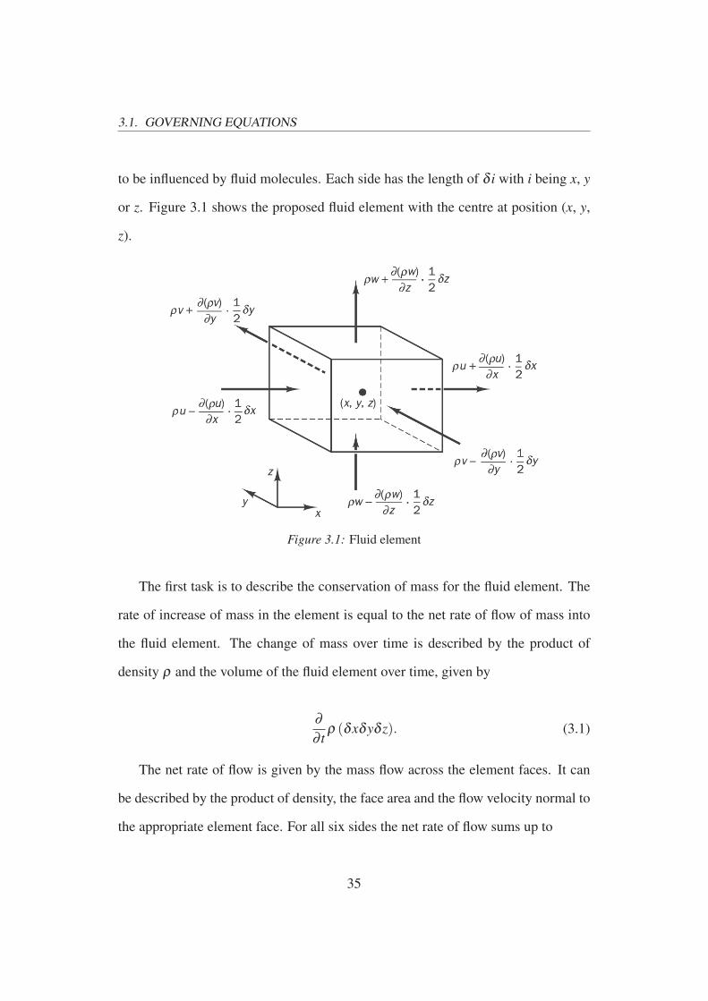
3.1. GOVERNING EQUATIONS
to be influenced by fluid molecules. Each side has the length of δ i with i being x, y
or z. Figure 3.1 shows the proposed fluid element with the centre at position (x, y,
z).
Figure 3.1: Fluid element
The first task is to describe the conservation of mass for the fluid element. The
rate of increase of mass in the element is equal to the net rate of flow of mass into
the fluid element. The change of mass over time is described by the product of
density ρ and the volume of the fluid element over time, given by
∂
∂ tρ (δxδyδ z). (3.1)
The net rate of flow is given by the mass flow across the element faces. It can
be described by the product of density, the face area and the flow velocity normal to
the appropriate element face. For all six sides the net rate of flow sums up to
35

3.1. GOVERNING EQUATIONS
(ρu− ∂ (ρu)
∂x
1
2δx
)δyδ z−
(ρu+
∂ (ρu)
∂x
1
2δx
)δyδ z
+
(ρv− ∂ (ρv)
∂y
1
2δy
)δxδ z−
(ρv+
∂ (ρv)
∂y
1
2δy
)δxδ z (3.2)
+
(ρw− ∂ (ρw)
∂ z
1
2δ z
)δxδy−
(ρw+
∂ (ρw)
∂ z
1
2δ z
)δxδy.
Equations 3.1 and 3.1 lead to the continuity equation for compressible flow,
∂ρ
∂ t+
∂ρu
∂x+
∂ρv
∂y+
∂ρw
∂ z, (3.3)
which reduces to
∂u
∂x+
∂v
∂y+
∂w
∂ z(3.4)
for incompressible flow, as the density is constant in this case. u, v and w are the
Cartesian velocity components. To describe the fluid flow further the momentum
equations need to be derived. The momentum equations are based on Newton’s
second law. That states that the rate of change of momentum of a fluid particle is
equal to the sum of the forces acting on it. The forces can be divided into surface and
body forces. Here, the pressure and viscous forces act on the surface and gravity,
the centrifugal, Coriolis and electromagnetic forces are known as body forces. Only
the surface forces will be included into the equations directly. The body forces will
be included in the source term. According to the statement for the conservation of
mass for a fluid element the equation for an arbitrary fluid property φ , which for the
momentum equation would be replaced with u, v and w for the momentum in x, y
36

3.1. GOVERNING EQUATIONS
and z direction, is written as
∂φρ
∂ t+
∂φρu
∂x+
∂φρv
∂y+
∂φρw
∂ z(3.5)
From the forces that act on the faces of the fluid element, i.e. those resulting
from the pressure and stress components, the momentum equations can be derived
for every coordinate direction separately. When multiplied by the face area they
represent the force. For the whole fluid element as shown in Figure 3.1 the net force
in one direction is the sum of all force components acting in that direction. For
the x-direction the components are shown in the following equations. Therefore the
force balance for forces in the x-direction is shown for each pair of opposing sides
of the fluid element. The forces in the x-direction on the two element faces normal
to the x-axis are
[(p− ∂ p
∂x
1
2δx
)−
(τxx −
∂τxx
∂x
1
2∂x
)]δyδ z
+
[−
(p+
∂ p
∂x
1
2δx
)+
(τxx +
∂τxx
∂x
1
2∂x
)]δyδ z
=
(−∂ p
∂x+
∂τxx
∂x
)δxδyδ z. (3.6)
τi j, with i and j being the Cartesian coordinates x, y or z, are the viscous stress
components acting in j-direction and normal to a surface in i-direction.
The x-forces on the faces normal to y-axis are
−(
τyx −∂τyx
∂y
1
2δy
)δxδ z+
(τyx +
∂τyx
∂y
1
2δy
)δxδ z
37

3.1. GOVERNING EQUATIONS
=∂τyx
∂yδxδyδ z. (3.7)
The x-forces on the faces normal to z-axis are
−(
τzx −∂τzx
∂ z
1
2δ z
)δxδy+
(τzx +
∂τzx
∂ z
1
2δ z
)δxδy
=∂τzx
∂ zδxδyδ z. (3.8)
All components, i.e. equations (3.6), (3.7) and (3.8), summed up and divided by
δxδyδ z give the total force per unit volume as
∂ (−p+ τxx)
∂x+
∂τyx
∂y+
∂τzx
∂ z. (3.9)
To finalise the equation for the momentum conservation the body forces need
to be added. These are included in the source term SMx. The same has to be done
for the remaining coordinate directions y and z. Equations (3.10), (3.11) and (3.12)
show the full set of momentum equations in non-conservative form.
∂ (−p+ τxx)
∂x+
∂τyx
∂y+
∂τzx
∂ z+SMx (3.10)
∂τxy
∂x+
∂ (−p+ τyy)
∂y+
∂τzy
∂ z+SMy (3.11)
∂τxz
∂x+
∂τyz
∂y+
∂ (−p+ τzz)
∂ z+SMz (3.12)
For the calculation of 3-dimensional incompressible flow four equations have been
described: the 3 momentum equations and the equation for the conservation of
38

3.1. GOVERNING EQUATIONS
mass. All are valid for Cartesian coordinates and developed from a fluid element
with sides of finite lengths δx, δy and δ z. The main unknown variables in these
expressions are the three velocity components u, v and w and the pressure p. This
set of four equations and four unknowns would be possible to solve. However, also
included in the momentum terms are the nine expressions for the viscous stress
components τi j. The definition for a Newtonian fluid says that the deformation of a
fluid element is direct proportional to the viscous stresses that act on it. As all gases
and most liquids, and certainly water, are isotropic, i.e. behave the same way in all
coordinate directions, the viscous stresses can be linked to the dynamic viscosity of
the fluid. The nine viscous stress components, of which six are independent, can
then be expressed by
τxx = 2µ∂u
∂x− 2
3µ
(∂u
∂x+
∂v
∂y+
∂w
∂ z
),
τyy = 2µ∂v
∂y− 2
3µ
(∂u
∂x+
∂v
∂y+
∂w
∂ z
),
τzz = 2µ∂w
∂ z− 2
3µ
(∂u
∂x+
∂v
∂y+
∂w
∂ z
),
τxy = τyx = µ
(∂u
∂y+
∂v
∂x
),
τxz = τzx = µ
(∂u
∂ z+
∂w
∂x
)
and
τyz = τzy = µ
(∂v
∂ z+
∂w
∂y
).
These being substituted into equations (3.10), (3.11) and (3.12) yield the Navier-
Stokes equations for incompressible fluids
39

3.1. GOVERNING EQUATIONS
∂u
∂x+
∂v
∂y+
∂w
∂ z= 0 (3.13)
∂uρ
∂ t+
∂ρu
∂x+
∂ρv
∂y+
∂ρw
∂ z=−∂ p
∂x+
∂
∂x
(µ
∂u
∂x
)+
∂
∂y
(µ
∂u
∂y
)+
∂
∂ z
(µ
∂u
∂ z
)+SMx
∂uρ
∂ t+div(ρuuuu) = −∂ p
∂x+div(µgrad u)+SMx (3.14)
∂vρ
∂ t+
∂ρu
∂x+
∂ρv
∂y+
∂ρw
∂ z=−∂ p
∂y+
∂
∂x
(µ
∂v
∂x
)+
∂
∂y
(µ
∂v
∂y
)+
∂
∂ z
(µ
∂v
∂ z
)+SMy
∂vρ
∂ t+div(ρvuuu) = −∂ p
∂y+div(µgrad v)+SMy (3.15)
∂wρ
∂ t+
∂ρu
∂x+
∂ρv
∂y+
∂ρw
∂ z=−∂ p
∂ z+
∂
∂x
(µ
∂w
∂x
)+
∂
∂y
(µ
∂w
∂y
)+
∂
∂ z
(µ
∂w
∂ z
)+SMz
∂wρ
∂ t+div(ρwuuu) = −∂ p
∂ z+div(µgrad w)+SMz (3.16)
The Navier-Stokes equations ((3.13), (3.14),(3.15) and (3.16)) share a number
of commonalities and can be re-written in the form of a general transport equation,
as
∂ (ρφ)
∂ t+div(ρφuuu) = div(Γgrad φ)+Sφ , (3.17)
which states that the rate of increase for an arbitrary fluid property φ , such as a
40

3.1. GOVERNING EQUATIONS
velocity component, temperature or the concentration of a transported element, per
fluid element (see Figure 3.1) plus the net rate of flow of the fluid element is equal
to the rate of increase of φ due to diffusion plus the change of φ due to sources (or
losses).
When equation (3.17) is integrated over a control volume (CV) it can be written
as
∫
CV
∂ (ρφ)
∂ tdV +
∫
CVdiv(ρφuuu)dV =
∫
CVdiv(Γgrad φ)dV +
∫
CVSφ dV . (3.18)
Applying Gauss’ divergence theorem1 and integrating with respect to time for
transient simulations results in the general integrated form of the transport equation:
∫
∆t
∂
∂ t
(∫
CVρφdV
)dt
︸ ︷︷ ︸transient term
+∫
∆t
∫
A
nnn.(ρφuuu)dA dt
︸ ︷︷ ︸convective term
=
∫
∆t
∫
A
nnn.(Γgrad φ)dA dt
︸ ︷︷ ︸diffusive term
+∫
∆t
∫
CVSφ dV dt
︸ ︷︷ ︸source term
(3.19)
The first term on the left-hand side is called the transient term, followed by the
convection term. On the right-hand side of the expression are the diffusion and
source term.
This set of partial differential equations (PDE) defines the base for the com-
putational methods used to calculate the unknown flow velocities u, v, w and the
pressure p. For this work, two different solver techniques have been applied. Both
use a mesh of finite elements, on which the calculation is performed . If the simu-
1Gauss’ divergence theorem states for a vector a∫
CV div(aaa)dV =∫A
nnn.aaadA , with nnn being the
vector normal to the surface dA . For a fluid element or a CV respectively this is equal to the sum
of the normal vectors times the appropriate face area building the surface of the control volume.
41

3.1. GOVERNING EQUATIONS
lation is 2-dimensional, it consists of quadliteral cells. For the 3-dimensional cases
mostly hexahedral cells are used. Therefore the PDEs need to be discretised in
time and space onto the mesh, i.e. the nodes, the element faces and volumes. The
aim is to receive a set of linear equations with the same number of unknowns and
equations, which can then be solved numerically.
42

3.2. SOLUTION OF THE GOVERNING EQUATIONS
3.2 Solution of the Governing Equations
The objective of this section is to outline the discretisation of the governing equa-
tions on a mesh of finite elements consisting of control volumes, element faces and
nodes to obtain a linear set of equations containing the same number of variables
and equations.
3.2.1 Discretisation of NSE
For unstructured meshes two ways exist to arrange the control volumes on the mesh.
They can be constructed using either a cell-centred or vertex-centred approach. In
a cell-centred arrangement the nodes are placed in the centre of the CV (Figure
3.2a), whereas in the vertex-centred method the nodes are placed on the vertices of
the mesh. For this method the CVs are generated from the sub-volumes defined by
the cell centroids and the mid points of the edges as it can be seen in Figure 3.2b.
Both of these methods are used implemented in the solvers employed for this work.
Due to a CV always having more vertices than centroids, the cell-centred method
requires slightly less computational storage than the vertex-centred arrangement
(Versteeg & Malalasekera 2007).
For the discretisation on any CV the transport equation (3.19) can be written as
∂
∂ t
(∫
CVρφdV
)+ ∑
ACV
∫
A〉nnni.(ρφuuu)dA = ∑
ACV
∫
A〉nnni.(Γgrad φ)dA +
∫
CVSφ dV .
(3.20)
nnni is the outward normal vector on the surface element, Ai of the CV as shown in
Figure 3.3 for a 2D CV. Equation (3.20) sums up all fluxes of the fluid property φ
43

3.2. SOLUTION OF THE GOVERNING EQUATIONS
(a) cell-centred CV (b) vertex-centred CV
Figure 3.2: CV arrangement
through the CV faces of one CV and thereby connects it to a group of grid points
that surround it. As only a few grid points participate in a given discrete equation, φ
influences only the solution in the immediate neighbourhood. When the number of
CVs in the domain becomes large, the discrete expressions are expected to converge
to the exact solution for the whole domain. By assuring that the continuity and mo-
mentum equation are satisfied for every CV, conservation of mass and momentum
for the whole domain is guaranteed. Assuming the face velocities of the CV are
known the convective term of the discrete transport equation (3.20) can be written
as
FCV = ∑A
nnni (ρφuuu)dA = ∑A
Fiφi (3.21)
where φi is the transported fluid property at the centre of the CV surface element
i and Fi is the convective flux parameter [kg/s]. Different methods are available
to construct the convective flux at the CV face from the values of the surrounding
nodes. Here, a second-order scheme is used. For the CV shown in Figure 3.4 the
convective flux across the East face is calculated as
44

3.2. SOLUTION OF THE GOVERNING EQUATIONS
Feφe =
Fe (φC +∆xCe ·∇φC) for Fe ≥ 0
Fe (φE +∆xeE ·∇φE) for Fe < 0.(3.22)
∇φi are the reconstruction gradients in the cells either side of the CV face e.
The computation of these will be described in Chapter 3.2.3. In Figure 3.4 N, S, E
and W represent the North, South, East and West nodes of the centre node C. Small
letters and subscripts stand for the CV faces and the flow in that direction. ∆x is the
distance in x-direction between te points indicated in the subscripts Ce and eE.
The same nomenclature is used for the vertex-centred CV arrangement. The
centre node C is surrounded by the nodes N, S, E and W , which stands for North,
South, East and West, as shown in Figure 3.5. The grey shaded area is the CV
enclosed by a number of integration points (◦) and constructed from the element
face centres of the surrounding cells. For this case the convective flux is calculated
as the sum of the fluxes at the integration points as
FCV = FC = ∑ip
nnnip (ρφuuuip) = ∑ip
Fipφip (3.23)
where subscripts ip denote iteration point and nip is the area vector of the sub-
face corresponding to ip as it can be seen from Figure 3.5. The convective flux needs
to be approximated from the neighbouring vertex values and has to be bounded and
accurate. Bounded means that for example the total flux across one cell from the
surrounding cells must not be larger than the cell volume and must be limited if
this occurs. This is achieved by blending between 1st and 2nd order differencing
schemes. The implemented method is described by Barth & Jesperson (1989). The
convective flux can be computed as
45

3.2. SOLUTION OF THE GOVERNING EQUATIONS
Fip = Fip,up +β ∇F ·RRR (3.24)
with Fip,up being the upwind vertex value of the convective flux and RRR the vector
from the upwind vertex to the integration point. ∇F is the best estimate of the solu-
tion gradient in the cell computed from the surrounding centroid data (see Chapter
3.2.3). The blending factor β needs to be calculated. For β = 0 the method is a
first-order upwind scheme, which is bounded but diffusive. For β = 1 the scheme
is a second order upwind scheme, but unbounded (Zwart et al. 2003, Zwart 2005).
To make it a bounded high resolution scheme β is calculated as close to 1 as possi-
ble and reduced when necessary to prevent over- and under-shoots of the solution.
Therefore β is calculated depending on the neighbouring vertex values. The first
step is the computation of the maximum and minimum values of the neighbouring
cells and the centre cell itself, i.e. βC and βnb. Then βi is calculated for each cell
vertex to get β i given by
β i =
min(
1,Fmax
C −FC
Fip,i−FC
), if Fip,i −FC > 0
min(
1,Fmin
C −FC
Fip,i−FC
), if Fip,i −FC < 0
1 if Fip,i −FC = 0
(3.25)
β is then taken as the minimum of β i. For the centre cell C shown in Figure 3.5
this is given by β = min(
β nw, β ne, ..., β ws, β wn
)to find the value that insures
the best level of accuracy and boundedness but also stability of the solution for this
cell during the calculation of the convective flux.
The diffusive term of equation (3.20) is given as
46

3.2. SOLUTION OF THE GOVERNING EQUATIONS
Figure 3.3: Surface element normal vector
DCV = ∑ACV
∫
A〉nnni.(Γgrad φ)dA , (3.26)
where nnni is the outward normal vector and (Γgrad φ) represents a diffusive flux
vector for the CV element face Ai. When the mesh is non-orthogonal corrections
have to be applied, which are described by Mathur & Murthy (1997a,b) and Ferziger
& Peric (2001). They introduce a cross-diffusion term, which is treated as a source
term, when the discretised equations are solved. The derivation of this term is also
described in Versteeg & Malalasekera (2007).
For the East face of the CV in Figure 3.4 the diffusive flux [kg/s] can be written
as
nnni.(grad φe Γe) = Γe
((φE −φC) · nnne
nnne~CE
nnne +
(grad φE −grad φC
2
)nnnC
)− (3.27)
Γe
(grad φE −grad φC
2~CE
nnne
nnne~CE
nnne
),
where Γe is the average of the cell values and (grad φi) are the gradients at the CV
centroids. ~CE is the vector from C to E.
47

3.2. SOLUTION OF THE GOVERNING EQUATIONS
Figure 3.4: Cell-centred discretisation scheme
N,S,E,W are the North, South, East and West nodes of the centre node C, small
letters and subscripts stand for the CV faces and flow in that direction
48

3.2. SOLUTION OF THE GOVERNING EQUATIONS
Figure 3.5: Vertex-centred discretisation
The solid lines represent the element boundaries, dashed lines divide the elements
into sectors. The solution unknowns such as u, v, w and p are stored at the mesh
nodes (•), surface fluxes are calculated at the integration points (◦). A CV is
constructed from the appropriate element sectors (grey shaded area).
49

3.2. SOLUTION OF THE GOVERNING EQUATIONS
3.2.2 Pressure-Velocity Coupling
For incompressible flow the pressure field cannot be calculated from equations of
state that link the pressures to the density or temperature but have to be calculated
from the relation to the velocities in the continuity and momentum equations. For
the co-located variable arrangement, where the unknowns are solved and stored at
the same locations, Patankar (1980) describes the so-called “checker-board” effect.
This phenomenon occurs when the face values, which are used to calculate the node
values, are interpolated linearly from values of the surrounding vertices only. When
discretising these equations, the influence of the centre node cancels out for the
calculation of the face fluxes and thereby the cell value is only dependent on the
surrounding cells. For the upwind cell the same problem occurs, which might give
a converged but non-physical solution of the pressure field. One remedy would be
to store the variables, such as the velocities and pressures, at different locations.
This is called a staggered variable arrangement. As this solution requires slightly
more memory and is not implemented in the solvers used for the calculations in the
following chapters it will not be discussed further. Patankar (1980) describes this
method for an iterative solver.
To overcome this problem Rhie & Chow (1982) developed a higher-order pressure-
velocity coupling method, which is widely used for co-located grid arrangements.
For the cell-centred CV with centre node C as in Figure 3.4, the face velocities for
the East face are interpolated as
50

3.2. SOLUTION OF THE GOVERNING EQUATIONS
ue =uP +uE
2+
1
2
(A ∆x
aC
+A ∆x
aE
)(pC − pE
∆x
)− 1
2
(A ∆x
aC
(∇pC)+A ∆x
aE
(∇pE)
)
(3.28)
3.2.3 Gradient Computation
The computation of the gradients can be done differently. First, a method is de-
scribed, which here is applied to the cell-centred FV approach. The approximation
of the gradients, which are used to calculate the cell values for any fluid property
φ involves three steps. First the unlimited reconstruction gradients are obtained.
These are used to evaluate the cell gradients to reconstruct the cell face values for
the computation of the diffusive and convective fluxes. To prevent the solution from
over- and undershoots, the reconstruction gradients need to be limited (or bounded).
Finally the cell gradients can be calculated from the limited reconstruction gradi-
ents.
The unlimited pressure reconstruction gradients (gradφ)unlimited are computed
using the weighted least squares method, which for the centre cell C in Figure 3.4
can be expressed as
(gradφ)unlimited =
[
∑f
(xnb − xC)⊗ (xnb − xC)
(xnb − xC) · (xnb − xC)
]−1 [
∑f
(φC −φnb)(xnb − xC)
(xnb − xC) · (xnb − xC)
]
(3.29)
with xC and xnb representing the centroids of cell C and the neighbour cell respec-
tively. f stands for a control volume face and φC and φnb represent the data values
for cell C and its neighbour, here the pressure. For all other variables the gradients
51

3.2. SOLUTION OF THE GOVERNING EQUATIONS
are approximated using Gauss’ method as described by
(gradφ)unlimited =1
VC∑
f
φ faaa f (3.30)
with φ f being the arithmetic mean of the appropriate adjacent cell given as
φ f =φC −φnb
2. (3.31)
The face value for any cell face centroid of the centre cell C can then be calcu-
lated using
φ f ,C = φC +(x f − xC
)· (gradφ)unlimited (3.32)
When calculating the cell values from the unlimited reconstruction gradients,
the cell values may exceed the face values. Thus the reconstruction gradients have
to be limited to bound the face values and ensure physical behaviour of the solution.
The limiting of the reconstruction gradients is described by Venkatakrishnan (1993).
For the centre cell C the limited reconstruction gradient is given as
(grad φ)limited = α (grad φ)unlimited , (3.33)
where α is given by
α = min(α f
)and α f =
2r f +1
r f
(2r f +1
)+1
. (3.34)
The calculation of r f depends on the maximum and minimum values of the neigh-
bouring cells, which are used to limit the face values. r f is given by
52

3.2. SOLUTION OF THE GOVERNING EQUATIONS
r f =
∆ f
φ maxC −φC
for ∆ f > 0
∆ f
φ minC −φC
for ∆ f ≤ 0,(3.35)
where
φ maxC = max(φC,φnb) , (3.36)
φ minC = min(φC,φnb) (3.37)
and
∆ f = φ f ,C −φC =(x f − xC
)(grad φ)limited . (3.38)
These limited reconstruction gradients are then used for the calculation of cell
gradients for all convected properties, such as u, v, w and p, which are needed in the
discrete continuity and momentum equations and for the pressure-velocity coupling.
Now the gradient for cell C of the fluid property φ can be calculated by
gradφ =1
VC∑
f
φ f ,C +φ f ,nb
2, (3.39)
where
φ f ,C = φC +(x f − xC
)(grad φ)C,limited (3.40)
and
φ f ,nb = φnb +(x f − xnb
)(grad φ)nb,limited . (3.41)
Rather than calculating the gradients using the procedure as described above, Schnei-
der & Raw (1987a,b), Hutchinson & Raithby (1986), Baliga & Patankar (1983,
1980) adapt a procedure traditionally used in a Finite Element approach by using
53

3.2. SOLUTION OF THE GOVERNING EQUATIONS
Figure 3.6: CV-FE shape function
shape functions to approximate the variation of a fluid property across the CV. This
detail defines the name of a blended FE-FV method, which is also called a Control-
Volume Finite Element (CV-FE) method. This method can be used for different
solver strategies and grid arrangements. Baliga & Patankar use a segragative iter-
ative solver such as SIMPLE with a staggered variable arrangement. Schneider &
Raw, Hutchinson & Raithby describe a fully coupled solution procedure which is
similar to the one outlined in Chapter 3.2.6 and co-located variables which are both
used in CFX.
As the solution variables are saved in the mesh nodes, it is necessary to calculate
gradients at the integration points. Here the CV-FE solver combines the FE with
the FV method by making use of shape functions, which are typical for the FE
approach. Across a mesh element a general flow variable φ varies as described by
φ =NNode
∑i=1
Niφi, (3.42)
with N being the shape function for node i and φi is the value of φ at node i. Fur-
54

3.2. SOLUTION OF THE GOVERNING EQUATIONS
thermore, the summation of the shape function over all element nodes gives unity
and the shape functions are used to calculate geometric quantities, such as the co-
ordinates of the integration points and surface area vectors nnn. Figure 3.6 shows
the geometry of the shape function for a hexahedral control volume and the local
coordinate components r, s and t. Ni is given by
N1 (r,s, t) = (1− r)(1− s)(1− t) , (3.43)
N2 (r,s, t) = r (1− s)(1− t) ,
N3 (r,s, t) = rs(1− t) ,
N4 (r,s, t) = (1− r)s(1− t) ,
N5 (r,s, t) = (1− r)(1− s) t,
N6 (r,s, t) = r (1− s) t,
N7 (r,s, t) = rst
and
N8 (r,s, t) = (1− r)st.
As in a standard FE approach, the shape functions are used to evaluate the spatial
derivatives of the diffusion terms and the pressure gradients.
55

3.2. SOLUTION OF THE GOVERNING EQUATIONS
3.2.4 Boundary Conditions
After assembling the discrete continuity and momentum equations for all interior
faces conservation is ensured for the interior CVs. For the domain boundaries, how-
ever, the corresponding elements will have surfaces that are not yet included. For
the cell-centred CV arrangement used for the FV solver the CV faces coincide with
the boundary, whereas the vertex-centred CV is cut in half by the domain bound-
ary. For all of these boundary elements the necessary data to solve the conservation
equations needs to be specified by means of interior face and cell data and boundary
values. As there are no further nodes outside the domain from which the data could
be interpolated the values close the linear equations and not introduce further un-
knowns. By doing this, the fluid is confined and initialised for every timestep by the
specifying face velocities and pressures at the CVs. For the simulations discussed in
this work, a velocity inlet, an opening, wall boundaries and symmetry planes were
used to define the problem.
At an inlet, the convective flux is known and specified in terms of the mass
flow or flow velocities. At wall boundaries and symmetry planes the convective
fluxes are zero and in the case of an outflow they are assumed to be independent
of the coordinate normal to the boundary. Furthermore, at a no-slip wall the fluid
velocities are equal to the wall velocity, which is zero in the case of a stationary
wall. This is also called a Dirichlet boundary condition. Here the normal viscous
stress is also zero. Both of these conditions need to be specified, as for the diffusive
flux, or viscous flux, the derivative in the discretised flux equation would be non-
zero. This is opposite to the symmetry plane, where the shear stress is zero but
the normal stress has a non-zero value. For the co-located variable arrangement the
56

3.2. SOLUTION OF THE GOVERNING EQUATIONS
pressures need attention at the boundaries as all the solution data is stored in the
same nodes. For the calculation of the pressure forces in the momentum equations
the boundary values are needed. For small pressure gradients as they occur in flow
parallel to a wall the values may be extrapolated from the interior nodes. For large
pressure gradients from body forces, as they occur from buoyancy, this method is
not accurate enough and large normal velocities in the vicinity of the boundary
would be the result. By calculating only the normal velocities from the continuity
equation or by refining the mesh locally this problem can be avoided (Ferziger &
Peric 2001). This often results in prism layers near bodies in the flow.
For the vertex-centred CV the solution domain boundary coincides with the two
subcontrol volumes of node C as it can be seen in Figure 3.7. The boundary is
shown as the thick solid line across which the flow is advected into domain. At the
appropriate boundary integration points (bip,2) the boundary flow of the property
φ is included to the CV balance of node C. σn and σt are the normal and tangential
stress components at the North and South boundary integration points bipn and
bips respectively. ∆x and ∆y with subscripts n and s are the distances in vertcial and
horizontal direction north- and southwards of C to the boundary of the CV.
For a scalar the convective and diffusive boundary conditions are obtained by
interpolating from the surrounding node values and then integrating them over the
CV as described for the interior faces. This procedure is straightforward (Schneider
& Raw 1987a). The velocities and pressures, however, are treated as a set and
not individually. Here, the boundary condition information is given as normal and
tangential information. By doing this the boundary information can be defined by
specifying
57

3.2. SOLUTION OF THE GOVERNING EQUATIONS
Figure 3.7: Boundary control volume for vertex-centred mesh arrangement
The boundary is represented by the thick solid line. For the grey shaded CV the
boundary condition informations are specified at the boundary integration points
(2), interior integration points are shown as (◦)
• the velocities (Inlet)
• the pressure and velocity direction (Outlet)
• the zero normal stress with zero tangential velocity (Wall)
• zero tangential stress with zero normal velocity. (Symmetry)
At the boundaries the conservation equations for mass and momentum are as-
sembled for all sides of the CV except for the boundary as a result of the discretisa-
tion procedure for all interior faces. In the case of the mass conservation the equa-
tions are closed by interpolation from the surrounding nodal values, as the mass
flow is known. From the pressure-velocity coupling the pressures are obtained and
58

3.2. SOLUTION OF THE GOVERNING EQUATIONS
no more information regarding the pressures is needed. In case of the momentum
equations, the convective, pressure and diffusive terms need special attention. The
convective term of the momentum equation is assembled in a similar manner to
the scalar and continuity equation, the pressures being interpolated from the nodal
values (Raw 1985). The diffusive boundary momentum Db including the pressure
and velocity components (superscripts p, u and v) depends on both the normal and
tangential viscous stress components, which in 2 dimensions are given as
Dupb = σn,bipn ∆yn +σn,bips ∆ys −σt,bipn ∆xn −σt,bips ∆xs (3.44)
Dvpb = −σn,bipn ∆yn −σn,bips ∆ys +σt,bipn ∆xn +σt,bips ∆xs (3.45)
These include the two unknown stress components in normal and tangential di-
rection for each of the bips. To resolve these, two boundary conditions are required,
which are defined by
aσn +bun + cp = d (3.46)
eσt + f (ut +gun) = h (3.47)
Here, the coefficients a−h are user-supplied constants, which are used to define
the boundary conditions as stated in the list above (Schneider & Raw 1987a).σ , u
and p with subscripts n and t are the normal and tangential stress components, ve-
locities and pressures. These are equivalent to velocity inlet, pressure outlet, open-
ing and symmetry boundary conditions. When a stationary no-slip wall boundary
is needed, the velocities and stresses are set to zero.
59

3.2. SOLUTION OF THE GOVERNING EQUATIONS
3.2.5 Interface Capturing
For the computation of multiphase flow and therefore the location of the fluid in-
terface different methods can be used as discussed in Chapter 2. Here, two high
resolution interface capturing (HRIC) schemes are described. Both rely on the Vol-
ume of Fluid (VOF) formulation, which originally was proposed by Hirt & Nichols
(1981). Here an additional equation for a scalar ci representing the volume fraction
of fluid i is solved. As the form of this equation is similar to the transport equation
it can be solved using the same methods as employed for the governing equations.
For the computation the fluids are assumed to be immiscible. In a CV with several
immiscible fluids present the pressure and velocity field is shared for all of them.
Thus the fluid properties of a single fluid are calculated as from the fluid properties
of its constituent phases and their volume fractions, such as
ρ = ∑i
ρici and µ = ∑i
µici, (3.48)
with ci = Vi/V . The transport equation for the volume fraction ci is given as
∂
∂ t
∫
V
cidV +∫
A
ci (uuu−uuug)dA =∫
V
ScidV (3.49)
The capturing of the interface separating the fluids, here air and water, is done
by a high-resolution compressive differencing scheme described by Ubbink (1997)
and Ferziger & Peric (2001). It is also known under the acronym CICSAM, which
stands for Compressive Interface Capturing Scheme for Arbitrary Meshes. It fol-
lows a donor-acceptor approach, where the boundedness is achieved using a Nor-
malised Variable formulation as introduced by Leonard (1991). The Normalised
60
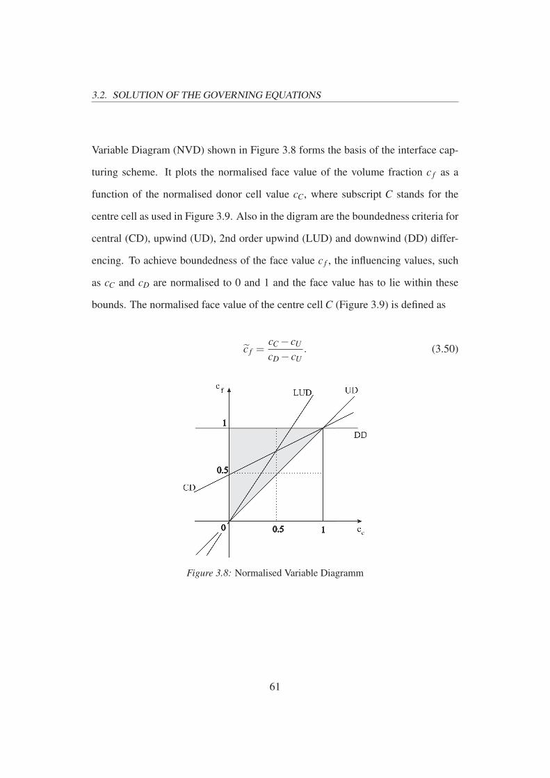
3.2. SOLUTION OF THE GOVERNING EQUATIONS
Variable Diagram (NVD) shown in Figure 3.8 forms the basis of the interface cap-
turing scheme. It plots the normalised face value of the volume fraction c f as a
function of the normalised donor cell value cC, where subscript C stands for the
centre cell as used in Figure 3.9. Also in the digram are the boundedness criteria for
central (CD), upwind (UD), 2nd order upwind (LUD) and downwind (DD) differ-
encing. To achieve boundedness of the face value c f , the influencing values, such
as cC and cD are normalised to 0 and 1 and the face value has to lie within these
bounds. The normalised face value of the centre cell C (Figure 3.9) is defined as
c f =cC − cU
cD − cU
. (3.50)
Figure 3.8: Normalised Variable Diagramm
61

3.2. SOLUTION OF THE GOVERNING EQUATIONS
Figure 3.9: CICSAM scheme
The normalised face value c f is calculated as
c f =
cC if cC < 0
2cC if 0 ≤ cC < 0.5
1 if 0.5 ≤ cC < 1
cC if 1 ≤ cC
(3.51)
To ensure that only such an amount of fluid leaves the donor cell as the acceptor
cell can accommodate or vice versa the calculated value of c f is corrected by using
the local Courant number Co. The new face value c∗f is calculated as
c∗f =
c f if Co < Col
cC +(c f − cC
)Cou−CoCou−Col
if Col ≤ Co < Cou,
cC if Cou ≤ Co
(3.52)
62
3.2. SOLUTION OF THE GOVERNING EQUATIONS
with
Co =uuu aaa
VC
. (3.53)
When the fluid interface as seen in Figure 3.9 is parallel to the flow direction the
downwind scheme tends to wrinkle. Therefore the previous results are corrected
once more by taking the orientation of the fluid interface into account. Here, θ ,
which is the angle between the normal of the fluid interface aaa and the cell-surface
vector nnn, is used as defined by
c∗∗f = c∗f√
cosθ + cC
(1−
√cosθ
). (3.54)
Finally the cell-face value is calculated as
c f = c∗∗f (cD − cU)+ cU . (3.55)
Subscripts U , C and D denote the upstream, cell-centre and downstream cell
values. Col and Cou are the lower and upper limits of the Courant number. For
values Co < Col HRIC is used, for Col < Co < Cou HRIC and UD are blended and
for Cou < Co UD is used.
The compressive characteristics of controlled downwinding schemes such as
CICSAM or other donor-acceptor methods (Ubbink 1997, Hirt & Nichols 1981)
depends upon the timestep. Therefore they require a small timestep to capture the
fluid interface sharply. Zwart (2005) and Zwart et al. (2003) describe another inter-
face capturing approach, where the compressiveness is independent of the timestep
length. The approach is similar to the advection scheme published by Barth & Jes-
person (1989) and described in Chapter 3.2.1. However, when the method is applied
63

3.2. SOLUTION OF THE GOVERNING EQUATIONS
to the volume fraction equation it causes too much numerical diffusion. The solu-
tion to this problem was found by allowing β > 1 (see equation (3.24)), but still
maintain the boundedness by reducing it as much as necessary to avoid under- and
overshoots. For the treatment of the volume fraction equation β is allowed to go
up to 2. As discussed earlier, the computation of the cell value is based on vertex
values of the surrounding cells. Hence it is not timestep dependent.
3.2.6 Solution Methods
Segregated Solver
The solution of the flow equations can be done in a segregated-iterative manner.
Here it is described for a co-located (non-staggered) variable arrangement combined
with the Rhie-Chow type pressure-velocity coupling as outlined in Chapter 3.2.2
(Rhie & Chow 1982) and a SIMPLE algorithm (Semi-Implicit Method for Pressure-
Linked Equations, Patankar (1980)).
The solution algorithm can be summarised starting from setting the boundary
conditions. Then the reconstruction gradients are computed as described in Chap-
ter 3.2.3 for the velocities and pressures in the flow field. From the reconstruction
gradients the velocity and pressure gradients are obtained and the discretised mo-
mentum equation are solved to create an intermediate velocity field u⋆. This veloc-
ity field is used to compute the uncorrected mass fluxes or convective fluxes at the
CV faces, F⋆Ai
. After that the pressure correction equations are solved to produce
cell values of the pressure correction p′, which is the used to update the pressure
field and the boundary pressure corrections. With the corrected pressure field the
mass fluxes at the CV faces can be corrected as well as the cell velocities. Then the
densities are updated due the pressure changes and the storage is freed.
64

3.2. SOLUTION OF THE GOVERNING EQUATIONS
Coupled Solver
Figure 3.10: Solution strategy for the coupled solver (ANSYS 2006)
Rather than using a “guess and correct” approach as described for the segregated
solver, which has the SIMPLE algorithm implemented, it is also possible to fully
couple the discrete hydrodynamic equations for u, v, w and p and solve them as a
65
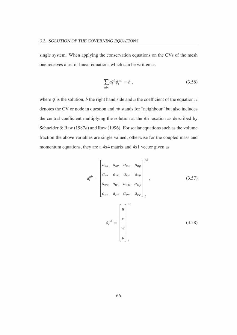
3.2. SOLUTION OF THE GOVERNING EQUATIONS
single system. When applying the conservation equations on the CVs of the mesh
one receives a set of linear equations which can be written as
∑nbi
anbi φ nb
i = bi, (3.56)
where φ is the solution, b the right hand side and a the coefficient of the equation. i
denotes the CV or node in question and nb stands for “neighbour” but also includes
the central coefficient multiplying the solution at the ith location as described by
Schneider & Raw (1987a) and Raw (1996). For scalar equations such as the volume
fraction the above variables are single valued; otherwise for the coupled mass and
momentum equations, they are a 4x4 matrix and 4x1 vector given as
anbi =
auu auv auw aup
avu avv avw avp
awu awv aww awp
apu apv apw app
nb
i
, (3.57)
φ nbi =
u
v
w
p
nb
i
(3.58)
66

3.2. SOLUTION OF THE GOVERNING EQUATIONS
and
bi =
bu
bv
bw
bp
nb
i
. (3.59)
The overall solution strategy for the CV-FE solver implemented in CFX is
schematically shown in Figure 3.10. The definition file of the simulation contains all
relevant data to start the simulation. The mesh values, such as the coordinates and
numbers of the nodes, the connectivity and 2D and 3D regions, such as the bound-
aries and bodies, are defined here. At each of these nodes the CV, integration points
are calculated and the velocities and pressures are initialized for the first timestep.
If mesh motion is included, this is solved afterwards, followed by the hydrodynam-
ics including the volume fractions of the fluids, additional variables, turbulence and
mass fractions. Most likely the convergence criteria is not satisfied after the first
iterations, meaning that the solution of the system of linear equations still differs
too much from the maximum specified error allowed. If so, the hydrodynamics
are iterated again within the timestep to improve the quality of the solution. For a
well defined simulation using the CV-FE solver it usually takes 2-4 inner iterations
before the solver advances in time.
Also included in Figure 3.10 are routines, which are not used in the process of
this work, such as the modules that solve radiation, energy, mass fraction and full
coupled particles. For the modelling of radiation different methods can be chosen
in CFX. These depend on the type of radiation. If the medium is transparent to
radiation at wavelengths in which the majority of heat transfer occurs, i.e. only the
boundaries of the domain are heated or cooled by the radiation, the Monte Carlo
67

3.2. SOLUTION OF THE GOVERNING EQUATIONS
model should be used. The more optically dense the medium becomes, the Rosse-
land Model (Siegel & Howell 1981) or P1 Model (Raithby 1991) can be chosen
instead.
For multiphase flow, such as modelled here using air and water, the volume
fractions are solved after the hydrodynamic system. In the module that solves the
mass fractions additional components such as smoke or pollutant can be solved,
which do not influence the flow field of the fluid in which they are transported.
This is valid for small to medium concentrations of such extra properties. When the
concentration becomes larger one can also use particle tracking, which is solved at
the end of the inner loop.
When turbulent flow is modelled, CFX solves the equations to close the Reynolds-
Averaged Navier-stokes equations after the solution of energy equations. Here, the
viscous stresses as described in Chapter 3.1 are calculated using for example:
• k− ε or k−ω Model
• Large Eddy Simulation (LES)
• Detached Eddy Simulation (DES)
• Shear Stress Transport (SST) Model
• Baseline (BSL) Model
However, when the SST or BSL turbulence model are selected, the wall distance
needs to be specified, which allows the solver to blend between the k− ε and k−ω
model. The wall scale region depending on these setting is solved at the beginning
of the time loop. (ANSYS 2006)
68

3.2. SOLUTION OF THE GOVERNING EQUATIONS
Finally, when the stopping criteria is reached, the solution is terminated and the
final results file is generated. Therefore the maximum number of timesteps or the
total runtime can be specified. Transient result files can be saved after each timestep
or at specified intervals. These contain all solution variables, such as the velocities
for each fluid fraction u, v, w and pressures p for every cell of the domain.
Depending on the size of the domain, i.e. the number of cells and nodes, the
disk space required to save one full transient simulation may be large and easily
exceed several hundred gigabytes.
69

Chapter 4
Wave-Wave Interaction
4.1 Regular Waves
Prior to the focused wave cases, which are described in Chapter 4.2, regular waves
were simulated in order to assess the suitability of the CFD methods for simulating
extreme waves. The advantage of regular waves over irregular and focused waves
is the simplicity in the setup. Regular waves should remain constant in shape and
height throughout the tank, whereas focused and irregular waves interact with one
another. This would make it difficult to judge, whether the results are correct or
whether mesh effects or general problems such as numerical difficulties have oc-
curred. For these reasons regular waves are used to investigate the performance of
the numerical wave tank (NWT).
4.1.1 Computational Domain for Regular Waves
The regular wave tests are carried out in a 3-dimensional NWT. According to the
description of the numerical methods in Chapter 3.2, the domain height is twice the
initial water depth as both air and water are simulated. The height and width of the
wavetank are both 3 m and the length is 35 m for the grid convergence study, and
100 m for the investigations of the damping in the NWT and the influence of the
cell on the solution of the free surface.
The boundary arrangement is shown in Figure 4.1. A velocity inlet is used to
70
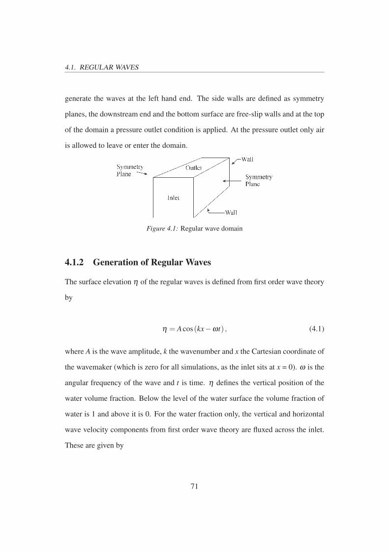
4.1. REGULAR WAVES
generate the waves at the left hand end. The side walls are defined as symmetry
planes, the downstream end and the bottom surface are free-slip walls and at the top
of the domain a pressure outlet condition is applied. At the pressure outlet only air
is allowed to leave or enter the domain.
Figure 4.1: Regular wave domain
4.1.2 Generation of Regular Waves
The surface elevation η of the regular waves is defined from first order wave theory
by
η = Acos(kx−ωt) , (4.1)
where A is the wave amplitude, k the wavenumber and x the Cartesian coordinate of
the wavemaker (which is zero for all simulations, as the inlet sits at x = 0). ω is the
angular frequency of the wave and t is time. η defines the vertical position of the
water volume fraction. Below the level of the water surface the volume fraction of
water is 1 and above it is 0. For the water fraction only, the vertical and horizontal
wave velocity components from first order wave theory are fluxed across the inlet.
These are given by
71

4.1. REGULAR WAVES
u =gAk cosh(k (z+h))cos(kx−ωt)
ω cosh(kh)(4.2)
and
w = −gAk sinh(k (z+h))sin(kx−ωt)
ω cosh(kh), (4.3)
where u is the horizontal and w the vertical velocity component. z is the Carte-
sian coordinate in the positive upward vertical direction and h is the still water depth.
The implementation of the inlet boundary conditions using different scripting ap-
proaches for the CFD codes is described in Chapter 4.2.3.
4.1.3 Grid Convergence Study
Figures 4.2 and 4.3 show short sections across the total domain height of the used
meshes for the grid convergence study for both solvers. For the segregated iter-
ative solver, which employs the FV approach and a cell-centred CV arrangement,
five meshes are used. Initially the simulations were done on a pure tetrahedral mesh,
then a pure polyhedral mesh and finally 3 hexahedral mesh arrangements were used.
The properties of the meshes are described in Table 4.1. The tetrahedral and poly-
hedral mesh are refined in the region of the free surface, i.e. 0.2 m above and below
the still water level. These showed a distorted solution of the captured fluid interface
due to the shape of the mesh elements such that the face geometry could be seen
on it. This finding led to the hexahedral meshes, where two degrees of refinement
in the same region are tested. The coarse mesh (Figure 4.2c) has 8 cells per wave
height with 5 cells above and below to resolve the remaining air and water fraction.
For the fine mesh (Figure 4.2d), the number of cells per wave height is increased to
72

4.1. REGULAR WAVES
14. The last mesh, which is not shown in the picture, investigates the effect on the
fluid interface solution due to refinement. Therefore the coarse mesh is used, where
only a section in the tank is refined to the level of the fine mesh. The results for the
hexahedral meshes for a regular wave with A = 0.15 m, λ = 15.19 m and T = 4.2 s
at a waterdepth h = 1.5 m are shown in Figure 4.4a.
The meshes used for the coupled solver (CFX) are shown in Figure 4.3, with
similar effects occurring for pure tetrahedral meshes, which led to the selection of
the combined tetrahedral-prism grids. Here, the tetrahedral mesh representing the
majority of the water and air fraction in the NWT is extruded towards the still water
level. This results in a prism layer around this region, where the influence from the
non-orthogonal vertices and faces of the pure tetrahedral mesh is reduced. Figure
4.4b shows the surface elevation results for the three meshes. The finer meshes
give the same results, whereas the coarse mesh (Figure 4.3a) differs from the mesh
independent solution. According to the findings in this section, the number of cells
per wave height was set to 10 or more for all subsequent simulations.
Figure 4.2: Mesh section of STAR CCM+ meshes
73

4.2. FOCUSED WAVES
Figure 4.3: Mesh section of CFX 5.7 meshes
4.1.4 Damping of Waveheight in the Numerical Wave Tank
Another issue to resolve is the damping of the waves with distance from the wave-
maker. For the wave-structure interaction cases it is important to know the shape
and height of waves at a given position in the tank. Figure 4.5 shows the surface
elevation in the tank for one timestep. The plot is shown for two different waves
with kh/kA = 1.96/0.06 and 0.62/0.2. Although the waves damp out at different
rates both waves have their defined height one wavelength behind the wavemaker.
This is the preferred location in the tank to put structures, such as the vertical and
horizontal cylinders, or the location to focus the extreme waves.
4.2 Focused Waves
In order to simulate an extreme wave of realistic profile for testing the survivability
of WECs, NewWave focusing as described earlier in Chapter 2 (Taylor 1992, Taylor
74

4.2. FOCUSED WAVES
(a) STAR CCM+
(b) CFX
Figure 4.4: Surface elevation at x = 10m
75

4.2. FOCUSED WAVES
Table 4.1: Mesh properties
Meshtype L/W/H[m] Cells vert. no. of cells
STAR CCM+ Tetrahedral 35/3/3 596124 27
Polyhedral 35/3/3 99087 16
Coarse hexahedral 35/3/3 100663 10/8
Fine hexahedral 35/3/3 543021 12/14
Partly refined hexa-
hedral
35/3/3 145280 12/14
Coarse hexahedral 100/3/3 286804 10/8
CFX Coarse tetrahedral-
prism
35/3/3 150480 2x4 tet./8 prism.
Fine tetrahedral-
prism
35/3/3 636386 2x8 tet./16 prism
Finest tetrahedral-
prism
35/3/3 1534058 2x9 tet./20 prism
Fine tetrahedral-
prism
100/3/3 1818200 2x8 tet./16 prism
Figure 4.5: Damping in the NWT
76

4.2. FOCUSED WAVES
& Williams 2002, 2004, Walker et al. 2004) is utilised.
4.2.1 Domain for Focused Waves
For the focused waves the wave tank geometry and set up used in the physical
experiments described in Ning et al. (2007) was followed. They used a wave tank
with plan dimensions of 69 m x 3 m and a water depth of 0.5 m. The waves were
generated by a piston wavemaker and wave reflections were absorbed by a 4 m foam
layer placed at the downstream end of the flume. Wave gauges (WG) were used to
measure the surface elevation around the point of the maximum wave elevation. In
the study by Ning et al. (2007), four NewWave cases are investigated with different
input amplitudes; here we reproduce numerically cases 2, 3 and 4 with kA = 0.2, 0.3
and 0.405 respectively.
The NewWave theory describes the surface elevation and wave velocity compo-
nents of a focused group of localised waves derived from a measured or theoretical
spectrum, such as JONSWAP or Pierson-Moskowitz. The waves are superposed
and brought into phase at one point in the tank at a specified time. This generates
an extreme wave event, which represents the wave environment of the underlying
spectrum. By increasing the input focused wave height, wave breaking at a defined
location can be achieved. However, with increasing wave height the waves become
more non-linear and the location where the waves focus or even break might vary
more significantly from the specified focus location and time in the wavemaker sig-
nal. In the physical experiment the focus point was set to 11.4 m downstream of the
wavemaker.
For both software packages similar domains are used as shown in Figure 4.6.
To save computational resources the domain is shortened to 13 m, following the
77

4.2. FOCUSED WAVES
approach taken by Ning et al. (2007) in their fully non-linear potential flow simu-
lations. The entire domain is 1m high with a water depth of 0.5 m. Between x =
10 m and x = 13 m, a damping layer is installed which prevents reflections from
the right-hand boundary. In this area the dynamic viscosity of the water fraction
increases linearly from 8.94 x 10⁻⁴ Pa s up to 1600 Pa s.
The left-hand boundary is a velocity inlet, where the horizontal and vertical
velocity components are applied together with the volume fraction of air and water.
These are calculated following the derivations described by Dalzell (1999), which
are extended to the number of wave components N required for this experiment.
The velocities are applied for the water fraction only and the velocity of the air
fraction at the inlet boundary is set to zero. The top boundary is a pressure outlet,
allowing only air to leave or enter the domain. The remaining boundaries at the
bottom and downstream end are walls. No turbulence model is applied.
The vertical coordinates where the water volume fraction is equal to 0.5 are
taken to be the position of the free surface and are extracted at different horizontal
positions in the tank for each time step. The results are given as surface elevation
time history plots and discussed in Sections 4.2.4 - 4.2.4 .
Figure 4.6: Computational domain
For the focused wave simulations, pure hexahedral meshes are used for the CFX
simulations. These pure hexahedral meshes became available in the software during
78

4.2. FOCUSED WAVES
the time of the project, but were not available for the early regular wave simulations.
However, due to the restrictions of the mesh generation software it was necessary
to use the same mesh resolution for the entire domain, which makes the simulations
expensive in relation to a partly refined mesh such as those used for the segregated
iterative solver. The simulations are done on a pseudo 2D mesh with one cell layer
thickness. For all NewWave cases the same mesh is used. According to grid conver-
gence studies, which are also published in Westphalen et al. (2007) and Westphalen
et al. (2008), the number of cells needed in the vertical direction is set to 110 over
the entire domain height. Thus for case kA = 0.2 the wave height is resolved by 14
cells in the vertical direction, this is sufficient to resolve the free surface accurately.
For case kA = 0.3 and 0.405 with A = 0.0875 m and 0.1031 m this gives 18 and 22
cells respectively.
For the wave cases with kA = 0.2 and 0.3 the timestep is set to 0.01 s. These
settings ensure a Courant number smaller than or close to 1. These settings resulted
in instabilities for the last NewWave case at the inlet. Here, the vertical motion of
the water surface per timestep due to the superposition of the N wave components
was too large for the cell size. By reducing the timestep to 0.005 s the issue could
be solved.
The calculations for the FV solver are carried out on a hexahedral mesh, which
is refined around the free surface similar to the ones shown in Figure 4.2. Due
to the increase in the expected wave height, the refined area is vertically extended
according to the linear target amplitude. Additionally the cells at the inlet are refined
for better definition of the velocity field and the rapidly moving free surface during
the calculation. The refined area ends at x = 6 m. Beyond that point the mesh is
uniform having the same cell size as the regions above and below the refined region.
79

4.2. FOCUSED WAVES
The calculation for case kA = 0.2 is made with a timestep of 0.001s. The two other
cases are started with the same timestep for the first 5s of the simulation reduces to
0.00025 s, for the same reasons as described for the coupled CV-FE solver (CFX).
4.2.2 Generation of Focused Waves
The concept of the NewWave formulation is to generate a number of waves of rel-
atively small amplitudes and range of periods (Taylor & Williams 2002, 2004).
These waves interact with one another and thereby build up a localised extreme
wave, larger than any individual wave created at the paddle, focused at a known
time and location in the tank. In the numerical calculations the waves are generated
from the spectra shown in Figure 4.7. These spectra are obtained by Fast Fourier
Transformation of the free surface data measured in the experiments as described
by Ning et al. (2007) and Zang et al. (2006).
For each wave component n the amplitude an is calculated as
an = ASn ( f )∆ f
∑N Sn ( f )∆ f(4.4)
where S( f ) is the spectral density, ∆ f is the frequency step depending on the
number of wave components N and bandwidth. A is the target linear amplitude
of the focused wave. Thus, the amplitude of every spectral component in the
NewWave group scales as the power density within that frequency band in the
assumed sea-state. Equivalently, NewWave is simply the scaled auto-correlation
function corresponding to a specified frequency spectrum such as JONSWAP or
Pierson-Moskowitz. The properties for each case considered are as shown in Table
80

4.2. FOCUSED WAVES
(a) kA=0.2 (b) kA=0.3
(c) kA=0.4
Figure 4.7: Input spectra for generation of focused wave group
Table 4.2: Properties of simulated cases
kA frange[Hz] N A [m] T [s]
0.2 0.6 - 1.3 16 0.0632 1
0.3 0.6 - 1.4 20 0.0875 1.25
0.405 0.5 - 1.8 16 0.1031 1.25
81

4.2. FOCUSED WAVES
4.2.
The underlying equations, from which the signal of the physical wavemaker is
derived, come from second order Stokes theory and are given by Ning et al. (2007)
and Dalzell (1999). The input signal for the CFD runs is the sum of the first (1)
and the second (2) order component for the horizontal and vertical water velocity
component u and w and the surface elevation η :
η = η(1) +η(2), (4.5)
u = u(1) +u(2) (4.6)
and
w = w(1) +w(2). (4.7)
The first order component for the surface elevation is
η(1) =N
∑i=1
ai cosψi (4.8)
where ψi is
ψi = kix−ωit + εi. (4.9)
k is the wavenumber, x the Cartesian coordinate, ω the angular frequency, t
is time and ε the phase angle (which is zero for all simulations). The first order
velocities u(1) and w(1) are
82

4.2. FOCUSED WAVES
u(1) =N
∑i=1
aikig
ωi
coshki (z+h)
coshkihcos(ki (x− x0)−ωi (t − t0)+ εi) (4.10)
and
w(1) =N
∑i=1
aikig
ωi
sinhki (z+h)
coshkihsin(ki (x− x0)−ωi (t − t0)+ εi), (4.11)
where x0 and t0 are the focus location and time and z is the vertical Cartesian coor-
dinate at the wavemaker.
The second order parts for the surface elevation η(2) and the velocities u(2) and
w(2) are given by
η(2) =N
∑i=1
∑j=i+1
aia jB+i, j cos
(ψi +ψ j
)+
N
∑i=1
∑j=i+1
aia jB−i, j cos
(ψi −ψ j
)
+N
∑i=1
a2jki
4tanh(kih)
[2+
3
sinh2 (kih)
]cos(2ψi)−
N
∑i=1
a2jki
2sinh(2kih)(4.12)
and
Φ(2) =N
∑i=1
∑j=i+1
aia jA+i, j
cosh((
ki + k j
)(z+h)
)
cosh((
ki + k j
)h) sin
(ψi +ψ j
)
+N
∑i=1
∑j=i+1
aia jA−i, j
cosh((
ki − k j
)(z+h)
)
cosh((
ki − k j
)h) sin
(ψi −ψ j
)
+N
∑i=1
a2i
3ωi
8
cosh(2ki + k jh
)
sinh4 (kih)sin(2ψi), (4.13)
83

4.2. FOCUSED WAVES
with components of the interaction kernels A+/−i, j , B
+/−i, j and D
+/−i, j defined as
A+i, j = −ωiω j
(ωi +ω j
)
D+i, j
[1− 1
tanh(kih) tanh(k jh
)]
+1
2D+i, j
[ω3
i
sinh2 (kih)+
ω3j
sinh2(k jh
)]
(4.14)
A−i, j =
ωiω j
(ωi −ω j
)
D−i, j
[1+
1
tanh(kih) tanh(k jh
)]
+1
2D−i, j
[ω3
i
sinh2 (kih)−
ω3j
sinh2(k jh
)]
(4.15)
B+i, j =
(ω2
i +ω2j
)
2g− ωiω j
2g
[1+
1
tanh(kih) tanh(k jh
)]
·[(
ωi +ω j
)2+g
(ki + k j
)tanh
((ki + k j
)h)
D+i, j
]
+
(ωi +ω j
)
2gD+i, j
[ω3
i
sinh2 (kih)+
ω3j
sinh2(k jh
)]
(4.16)
B−i, j =
(ω2
i +ω2j
)
2g+
ωiω j
2g
[1− 1
tanh(kih) tanh(k jh
)]
·[(
ωi −ω j
)2+g
(ki − k j
)tanh
((ki − k j
)h)
D−i, j
]
+
(ωi −ω j
)
2gD−i, j
[ω3
i
sinh2 (kih)−
ω3j
sinh2(k jh
)]
(4.17)
84

4.2. FOCUSED WAVES
D+i, j =
(ωi +ω j
)2 −g(ki + k j
)tanh
((ki + k j
)h)
(4.18)
and
D−i, j =
(ωi −ω j
)2 −g(ki − k j
)tanh
((ki − k j
)h)
(4.19)
The second order velocity components are obtained by the relevant spatial deriva-
tives of the second order potential Φ(2) to be differentiated with respect to x and z
in order to get the second order contribution to the inlet signal.
The x-coordinate is zero for the calculations, because the wavemaker sits at x =
0 m; x0 is the focus location, which is set to 3 m for case kA = 0.2 and to 3.27 m for
both other cases; t is the time; t0 is the focus time, which is 9.2 s for case kA = 0.2
and 10s for the others. Also in the formulae are the wavenumber ki, the frequency
ωi , the phase angle εi (which is set to 0 for the calculations), the water depth h,
vertical position z and the number of wave components N.
For the simulations as presented here, the incoming wave entering the compu-
tational domain is fluxed in through a transparent boundary. This flux is defined in
terms of either linear theory, or linear theory with second order corrections.
4.2.3 Implementation of Boundary Conditions
The implementation of the boundary condition is dependent on the user interface
of the commercial software package. Both software packages use their own script
languages to express simple mathematical equations and logical operations. Addi-
tionally, both also provide a user programming facility for more complex require-
ments. These offer more power and flexibility as they use traditional programming
languages and thereby benefit from their libraries. In the case of CFX, the user can
85

4.2. FOCUSED WAVES
programme a script in FORTRAN or PERL. STAR CCM+ uses Java and C++. As
described earlier, for both packages a velocity inlet was chosen, where the horizon-
tal and vertical velocity components need to be specified. Furthermore, the volume
fraction, representing the surface elevation arising from the wave equations needs
to be set. The wave velocities however, as the inlet reaches over the whole domain
height including the air fraction, need to be restricted to the water fraction only.
Otherwise one would experience a wind blowing in the domain as well. Thus there
exist two requirements to the setup:
• Definition of the velocities using the internal script language or the user pro-
gramming facility of the package
• Restriction of the velocities to the water fraction only
For simple mathematical equations and fairly short strings the internal script
language is used. This approach is valid for regular waves, such as given by equa-
tions (4.1), (4.2) and (4.3) and 1st order focused waves as given by equations (4.8),
(4.10) and (4.11). Here, u, v and η can be entered directly. Then these expressions
are treated by a logical operation using the script language, which restricts the ve-
locities to the water fraction defined by the position of the water volume fraction
= 0.5, which is equivalent to the surface elevation η . For every cell at the inlet
boundary, this operation can be expressed in words as follows:
• If the difference of water-fraction and air-fraction in the cell is positive, then
multiply the velocity expression by 1 and apply at the boundary cell face,
otherwise multiply by 0 and apply.
86

4.2. FOCUSED WAVES
The reason for the use of the user programming facilities can either be that the
string gets too long or difficult operations need to be carried out, such as iterations
or other methods in order to receive the full boundary condition expression. Here,
the velocity components and surface elevations including the second order contribu-
tions are calculated in a Java macro and a FORTRAN routine for STAR CCM+ and
CFX respectively. The way both packages incorporate such user scripts is different
and can be seen in Figure 4.8. The CFX solver is started and communicates several
times during the timestep loop with the script and passes the variables, which are
needed to calculate the wave equations to the script, i.e. the time and the z coordi-
nate at the inlet. The FORTRAN routine returns a single number for the appropriate
boundary cell which is then multiplied with the restriction expression.
The STAR CCM+ solver process on the other hand is started and controlled from
the Java macro. The macro is called once before the timestep and updates the solver
file with the expressions for the velocity components and surface elevations. These
are still strings, but can be simplified as much as possible within the Java macro. As
the time is known for every timestep beforehand, only the vertical variable is left
unknown and passed on to the solver. Then the boundary values are calculated as
described before.
For further interest, example scripts used for the generation of the waves in
STAR CCM+ and CFX are given in the Appendix.
87

4.2. FOCUSED WAVES
Figure 4.8: User scripting in STAR CCM+ and CFX
4.2.4 Focused wave results
Case 1, kA = 0.2
In total 16 simulations using the segregated iterative FV and coupled CV-FE solvers
were performed in order to compare the surface elevations at the focus point with the
experimental results by Ning et al. (2007). For both solvers, results are shown that
correspond to input waves defined using linear and linear plus second order theory.
The surface elevations are non-dimensionalised in terms of the linear amplitude of
the target NewWave A, and time is defined in terms of the appropriate central wave
period T , as shown in Table 4.2. Table 4.3 shows the maximum surface elevations
for these cases. As the actual focus point and time differ for every simulation, the
results are shifted in time to coincide with one another. They are adjusted at t/T =
88

4.2. FOCUSED WAVES
Table 4.3: Maximum surface elevations of focused waves
CV-FE (CFX) FV (STAR CCM+) Phys. Exp.
Elev. Dist. Elev. Dist. Elev. Dist.
Case 21st Ord. 1.08 3.0 m 0.93 2.61 m NA NA
2nd Ord. 1.12 3.68 m 1.24 3.29 m 1.03 3.0 m
Case 31st Ord. 1.13 3.68 m 1.17 3.68 m NA NA
2nd Ord. 1.17 4.08 m 1.23 4.08 m 1.10 3.29 m
Case 41st Ord. 1.07 3.68 m 1.26 3.68 m NA NA
2nd Ord. 1.27 3.0 m 1.28 3.68 m 1.22 3.29 m
0, which is taken as the time when the maximum surface elevation occurs. Figures
4.9 - 4.11 show the water surface elevation from the two solvers compared with the
physical experiment for all crest focused cases.
For a wave steepness of kA = 0.2, the case of the weakest non-linearity, the
segregated iterative solver with first order wave input signal (Figure 4.9a) does not
reach the required height. The simulation including the second order wave com-
ponents, however, overestimates the crest elevations by approximately 24%, with
a value of 0.015 m for an input amplitude of 0.0632 m. The trough elevations for
the surrounding troughs improve from first order to first plus second order wave
setup for the FV solver in terms of matching with the physical experiments. Figure
4.9b shows that the coupled solver predicts surface elevations for both wave signals
slightly higher than those measured in the physical tank tests. Here the troughs that
surround the central wave are higher and do not exactly coincide with the results of
the experimental results, although one can see an improvement from first order to
second order wave signal.
89

4.2. FOCUSED WAVES
(a) FV (STAR CCM+)
(b) CV-FE (CFX)
Figure 4.9: Surface elevation at focus point for kA = 0.2 (Case 2)
90

4.2. FOCUSED WAVES
Case 2, kA = 0.3
The numerical results for case kA = 0.3, presented in Figure 4.10, generally show
the best agreement with the physical experiments; particularly the central crest el-
evations are predicted with only a slight difference for both input signals. Moving
from first to second order wave input also improves the trough elevations.
Case 3, kA = 0.405
This case is the test with the steepest wave, which almost broke in the physical
experiment. The numerical results are very good for the maximum crest elevations.
However, the surrounding wave train does not agree as well as the previous tests,
though the trends are the same, as can be seen in Figure 4.11. The wave preceding
the central wave is much larger than the measured values for both codes, but still
smaller and not symmetric to the wave that follows the main wave, as can also be
observed in Figure 4.11.
The actual focus point in the numerical calculations lies further downstream than
specified, as can be seen from Table 4.3. Also, it is further away for the simulations
with higher order wave signal.
4.2.5 Non-linearity of Focused Waves
A useful tool to asses the linearity of results is the comparison of the sum and dif-
ference plots. Therefore additional simulations have to be carried out, with trough
focused instead of crest focused waves. By subtracting and summing the appropri-
ate time histories (and dividing them by two) the plots for cases kA = 0.2 and 0.405,
shown in Figure 4.12, are obtained. The difference represents the linear part of the
91

4.2. FOCUSED WAVES
(a) FV STAR CCM+)
(b) CV-FE (CFX)
Figure 4.10: Surface elevation at focus point for kA = 0.3 (Case 3)
92

4.2. FOCUSED WAVES
(a) FV (STAR CCM+)
(b) CV-FE (CFX)
Figure 4.11: Surface elevation at focus point for kA = 0.405 (Case 4)
93

4.2. FOCUSED WAVES
(a) Case 2
(b) Case 4
Figure 4.12: Sum and difference plots for the CV-FE solver (CFX)
94

4.2. FOCUSED WAVES
solution plus the odd harmonics and the sum is composed from the even harmonics
of the wave time history. As expected, the non-linearities increase from kA = 0.2 to
the steeper and thereby more non-linear case with kA = 0.405.
The sum and difference plots can then be analysed by performing a FFT. This
gives the frequency spectrum of the even and odd components in the processed
signal. Figure 4.13 shows the FFT results for the kA = 0.2 focused wave group.
The wave frequencies contributing to the linear signal plus the odd harmonics can
be identified through the peaks around 0.87 Hz and 2.7 Hz in Figure 4.13a. By
applying a bandpass filter for these frequencies to the difference data from Figure
4.12, the linear signal, shown as the dashed line in Figure 4.14a and the 3rd order
harmonics, seen as solid line in Figure 4.14a, can be separated from the difference
signal. The same procedure is applied to the even harmonics, which peak at 0.09
and 1.66 Hz. The bandpass filtering of the sum data results in the half and double
frequency second order components shown in Figure 4.14b. It should be noted that
the vertical axis scale of both graphs is different. The linear component contributes
almost 95 % to the overall wave elevation for the wave steepness kA = 0.2. The
second harmonics contribute approximately 4 % each and the third about 1 % to the
signal.
The same procedure has been applied to the appropriate data of the steepest
NewWave case with kA = 0.405. Here, the spectra obtained through FFT from the
sum and difference plots (Figure 4.12b) can be seen in Figure 4.15. For this case the
linear part can be identified at 0.87 Hz, whereas the third harmonic is more difficult
to spot in Figure 4.15a. It is taken to peak at 2.53 Hz. The 2nd harmonics can be
seen in Figure 4.15b peaking at 0.097 and 1.75 Hz.
Using these values for the bandpass filter applied to the sum and difference data
95

4.2. FOCUSED WAVES
results in the graphs shown in Figure 4.16. For this more non-linear case the linear
part only adds 80 % to the total wave elevation time history. Both 2nd harmonics
account for approximately 15 % each of the free surface elevation signal at the focus
point.
96

4.2. FOCUSED WAVES
(a) Linear part and odd harmonics
(b) Even harmonics
Figure 4.13: Spectra from difference (a) and sum plots (b) , kA = 0.2, Case 2
97

4.2. FOCUSED WAVES
(a) Linear part and odd harmonics
(b) Even harmonics
Figure 4.14: Filtered difference (a) and sum (b) results , kA = 0.2, Case 2
98

4.2. FOCUSED WAVES
(a) Linear part and odd harmonics
(b) Even harmonics
Figure 4.15: Spectra from difference (a) and sum plots (b) , kA = 0.405, Case 4
99

4.2. FOCUSED WAVES
(a) Linear part and odd harmonics
(b) Even harmonics
Figure 4.16: Filtered difference (a) and sum (b) results , kA = 0.405, Case 4
100

Chapter 5
Wave-Structure Interaction
In this section the problem considered is the fluid structure interaction between reg-
ular waves and horizontal and vertical cylinders. The waves used for the cylinder
computations are first order accurate as described in the publications by Dixon et al.
(1979) and Kriebel (1998), with which they are compared. Here, the vertical and
horizontal forces on the cylinder are of interest and the interplay of buoyancy and
inertial force is discussed. A special case in the paragraph about the vertical cylinder
is the section about excitation of the cylinder (Section 5.1.3). The so-called “ring-
ing” effect will be shown in the results. Additionally the force and resulting surface
elevations from the driven motion of an oscillating cone on the water surface are
investigated. The motion of the cone is not influenced by the pressure and viscous
forces from the water. The simulations involve mesh motion through deformation
of the cells in the vertical direction as the cylinder oscillates vertically during the
simulation.
5.1 Vertical Cylinder
This section describes the numerical simulations of a vertical cylinder in two regular
wave environments. The first set of tests reproduces the measured results in physical
experiments by Kriebel (1998). Kriebel compares the horizontal forces on a vertical
circular cylinder in regular waves with computations using first and second order
diffraction theory. From this publication two cases are chosen as described in Table
101

5.1. VERTICAL CYLINDER
5.1. k is the wavenumber, A the wave amplitude, h the water depth and T the wave
period. Furthermore, results of a slender vertical cylinder in steep waves of about
the same diameter as wave height are discussed.
Table 5.1: Properties of Vertical Cylinder Simulations
Simulation
1 2
kA 0.09 0.34
kh 1.61 1.61
NKC 0.32 0.54
A [m] 0.053 0.088
T [s] 1.95 1.05
5.1.1 Computational Domain
The numerical wavetanks (NWT) for the CFX and STAR CCM+ are identical. The
simulations are performed in a 3-dimensional domain with the dimensions x, y and
z equal to 12, 1.65 and 0.9, with z being the vertical direction as shown in Figure
5.1. The still water level is 0.45 m. The diameter of the cylinder is 0.325 m as
in the physical experiments. The centre of it is located 3.77 m downstream from
the inlet, which is equal to 1 wavelength for the first wave setup and approximately
2 wavelengths for the second. This distance was shown to work best for different
wave environments in Chapter 4.1.4.
As for the wave-wave interaction cases the waves are generated using the hor-
izontal and vertical velocity components, which are applied underneath the appro-
priate surface elevations at the left hand side velocity inlet. The sides are symmetry
planes and the top is a pressure outlet, with air being allowed to leave or enter the
102

5.1. VERTICAL CYLINDER
domain. The remaining boundaries are modelled as walls, i.e. the cylinder, the
bottom and the far end boundary.
The meshes, however, are different for each of the solvers and are shown in
Figure 5.2. The grid that is used for the coupled solver contains 570,000 hexahedral
cells. It is refined around the cylinder and the area where the free water surface is
expected to travel, upstream of the cylinder. Downstream of the cylinder the mesh
is relatively coarse to save computational resources. The cell size around the free
surface upstream of the cylinder is 0.011 m. The cylinder is discretised by 3240
quadrilateral elements. The number of cells covering the perimeter is 72, which is
the same over the entire cylinder height. The refinement of the cylinder in the area
where the waves hit the structure is in the vertical direction only. The timestep for
the CV-FE solver (CFX) is 0.005 s.
Figure 5.1: Numerical wavetank for vertical cylinder
The mesh used for the FV solver (STAR CCM+) contains 870,000 mostly hex-
ahedral cells. The cells around the water surface area are isotropically refined to an
edge length of 1.25 cm, which gives the necessary resolution of approximately 10
cells per wave height (Westphalen et al. 2008). The cylinder itself is modelled with
3005 faces, of which 37 are triangular, 2898 quadrilateral and 70 polygonal. The
different cell types result from the meshing algorithm, which cuts the geometry out
of the initial hexahedral mesh rather than using a body fitted grid as it is done for
103

5.1. VERTICAL CYLINDER
(a) CFX (b) STAR CCM+
Figure 5.2: Mesh around large vertical cylinder
the CV-FE solver. At the top and the bottom the cylinder contains 52 faces around
the perimeter. In the centre region of the cylinder the mesh is refined not only in the
vertical direction, as it is done for the CV-FE solver, but also tangentially. Between
the vertical positions of 0.35 m and 0.55 m 104 cells wrap the cylinder perimeter.
The mesh used for the CV-FE solver (CFX) is body fitted. Here, the hexahedral
cells are deformed around the cylinder to coincide with the geometric requirements.
This does not affect the orientation of the vertices in the vertical and longitudinal
direction and therefore the solution of the free surface around the structure is unaf-
fected.
The mesh used for the FV solver uses a cut-cell approach. The initial surface
mesh is built of tetrahedral cell from which the initial volume mesh consisting en-
tirely of hexahedral cells is generated. The structure, here the vertical cylinder,
is cut out of the initial volume mesh which results in the polygonal, quadrilateral
104

5.1. VERTICAL CYLINDER
and triangular faces representing the geometry. Figure 5.2b shows the mesh in the
vicinity of the large cylinder for the segregated iterative FV solver. As the region
of interest lies near the cylinder, the downstream part (right side of the cylinder in
the figures) of the tank can be modelled using a relatively coarse mesh. This sup-
ports the damping layer at the end of the NWT by introducing additional numerical
damping to prevent wave reflections from the downstream wall. The coarsening to-
wards that region is shown in Figure 5.3. The mesh used for the segregated iterative
solver (Figure 5.3a) employs a 1 cell - 2 cell/1 face - 2 face approach, whereas the
mesh for the coupled solver requires the arrangement shown in Figure 5.3b. Here,
one cell refines to three cells with every cell face coinciding with one neighbour cell
face. In three dimensions the coupled solver still requires that each cell face is met
by one neighbouring cell face. If the refinement does not meet these properties, the
faces between non-matching cell regions are defined as internal interfaces, which
might result in numerical inaccuracies when calculating the flow across the faces.
The FV solver can deal with anisotropic refinement in 3 dimensions. One cell can
sit next to 2 or 4 cells. The face area, however, must be the same for the coarse cell
compared to the sum of the refining cells.
5.1.2 Results of vertical cylinder case
The validation of the codes is achieved by comparing the predicted horizontal forces
on the cylinder due to the waves with the experimental results from Kriebel (1998).
As described by Kriebel the forces are normalised by the analytic results from linear
105

5.1. VERTICAL CYLINDER
(a) FV (STAR CCM+) (b) CV-FE (CFX)
Figure 5.3: Mesh refinement for both codes
diffraction theory, resulting in
F
F0= F
kh
ρgaHh tanhkd, (5.1)
where F is the measured or extracted horizontal force on the cylinder, F0 is the force
from diffraction theory, g is the acceleration due to gravity, ρ the water density, a
the radius of the cylinder, H the waveheight, k the wavenumber and h the still water
level (Sarpkaya & Issacson 1981).
Figure 5.4 shows the comparison between the experimental data and the two
numerical simulations for both wave regimes investigated. Both numerical methods
show good agreement for both cases, slightly better for the second one with kA =
0.34 and NKC = 0.54 (Figure 5.4b). Small differences in the results are expected
because the physical data is averaged over 10 wave periods, whereas the numerical
results represent one wave cycle only. For the second case (Figure 5.4b), for which
NKC is larger, the drag forces are more important than for the first wave environment
and as a result the physical experiments and the simulations reach a maximum value
106

5.1. VERTICAL CYLINDER
(a) kA = 0.09, NKC = 0.32
(b) kA = 0.34, NKC = 0.54
Figure 5.4: Horizontal forces on large vertical cylinder for both wave environments
107

5.1. VERTICAL CYLINDER
(a) Presented by Chaplin et al. (1997) (b) Simulated by using the FV solver
Figure 5.5: Secondary load cycle
almost twice as much as predicted by linear diffraction theory. This shows the limits
of linear methods in certain wave regimes.
5.1.3 Slender vertical cylinder and ringing of cylinder
A highly non-linear phenomenon is the so-called “ringing” of a vertical cylinder due
to interactions with steep waves. This effect was discovered during the design of a
large Norwegian oil rig in the 1990s (Stansberg 1997). Such tension leg or gravity
based platforms, constructed from vertical cylinders, may be affected by waves with
a period approximately 3-5 times larger than the resonance period of the structure.
Usually resonance occurs at 3-5 s. Grue et al. (1994) describe physical tank tests
of a vertical cylinder that is passed by transient wave groups of varying amplitudes.
For the wave groups with large wave height at the cylinder they found secondary
oscillations in the horizontal force measurements similar to the ones shown in Fig-
108

5.1. VERTICAL CYLINDER
ure 5.5. The oscillations start when the wave is about one cylinder diameter behind
the cylinder and last for 15 % of the wave period. The magnitude of the peak of
the oscillation to the peak of the total force was found to be 11 %. Grue et al.
also identified a low-pressure zone behind the cylinder, which they link to a suction
force. Besides describing the problem in terms of the non-dimensional Keulegan-
Carpenter and Reynolds numbers, Grue et al. state that the Froude number, given
as
NFr =u√gD
, (5.2)
with u being the particle velocity underneath the wave crest, g acceleration due
to gravity and D the cylinder diameter, is important. As the time when the crest
passes the structure is short, the problem is considered as a slowly varying hori-
zontal current. Then u can be estimated as u = Hω , where H is the local wave
height and ω the local wave frequency. For NFr = 0.4 the effect of the secondary
oscillations becomes pronounced.
The ringing itself only occurs when the cylinder is mounted elastically, which
is not the case for the simulations presented here. However, Chaplin et al. (1997)
have carried out tank tests to reproduce this effect. First they studied fixed vertical
cylinders in steep focused waves and then cylinders mounted elastically in order to
measure the excitation. Thus they were able to identify secondary loading within the
measured force curve. Chaplin et al. (1997) present the definition of the secondary
load cycle reproduced in Figure 5.5a, where the horizontal force on the cylinder
is plotted against time. They state that this effect occurs when the wave height is
equal to the cylinder diameter. Using the FV solver the horizontal force predicted
109

5.1. VERTICAL CYLINDER
(a) (b)
(c) (d)
Figure 5.6: Surface elevation around slender cylinder (Rainey & Chaplin 2003)
for a slender cylinder of diameter equal to 0.1625 m in the same wave climate as
described above can be seen in Figure 5.5b. The secondary load cycle is present
for this wave, although it cannot be compared exactly with Figure 5.5a as the inlet
wave condition is different. The secondary load cycle is initiated by the backward
breaking wave behind the cylinder. Photographic footage from tank tests published
by Rainey & Chaplin (2003) can be seen in Figure 5.6. In the first picture (a) the
waterlevel is almost at still water position followed by the approaching wave in the
next picture (b). Then the wave passing the cylinder axis is captured (c) and also
the backward breaking wave is shown (d). Furthermore, Rainey & Chaplin provide
110
5.2. HORIZONTAL CYLINDER
computational results of the free surface obtained from potential flow calculations.
The surface is accurately resolved for the wave passing the cylinder. However, the
highly non-linear effects of the wave breaking behind the vertical cylinder and also
the wave run-up upstream of the structure cannot be captured. Figures 5.7 - 5.10
show the surface elevations calculated by the FV solver at the same instances in
time from two perspectives: on the left-hand side the view is towards the negative
x-direction (back of the cylinder) and on the right-hand side the cylinder is seen
from an upstream position. Here, the wave run-up can be seen at t/T = 0.4-0.6,
which is resolved well. Also the breaking wave responsible for the secondary load
cycle can be seen at t/T = 0.8. Furthermore, highly non-linear processes appear at
the cylinder at t/T = 0.7, when the run-up water collapses sideways.
5.2 Horizontal Cylinder
In the following section the numerical results for a fixed horizontal cylinder in reg-
ular waves and three levels of submergence are presented. They are compared with
experimental results from Dixon et al. (1979). In the first simulation the horizontal
cylinder is placed at the free surface being half-submerged. Then the structure is
positioned deeper in the water with only 25% above still water level. At last the
cylinder sits fully submerged but close to the water surface in the tank. The water
depth h for all numerical simulations is 1 m, the wave period T is 1.646 s with wave
amplitudes A being 0.125 m, 0.05 m and 0.075 m. The diameter of the cylinder D is
0.25 m. Further properties: the displacement of the cylinder from still water level d,
kA, kh and the Keulegan-Carpenter numbers NKC for each case are shown in Table
111

5.2. HORIZONTAL CYLINDER
(a) t/T = 0.0
(b) t/T = 0.2
Figure 5.7: Surface elevation around slender cylinder
112

5.2. HORIZONTAL CYLINDER
(a) t/T = 0.3
(b) t/T = 0.4
Figure 5.8: Surface elevation around slender cylinder
113

5.2. HORIZONTAL CYLINDER
(a) t/T = 0.6
(b) t/T = 0.7
Figure 5.9: Surface elevation around slender cylinder
114

5.2. HORIZONTAL CYLINDER
(a) t/T = 0.8
(b) t/T = 1.0
Figure 5.10: Surface elevation around slender cylinder
115

5.2. HORIZONTAL CYLINDER
Table 5.2: Properties of Horizontal Cylinder Simulations
Simulation
1 2 3
d [m] 0.0 -0.075 -0.15
kA 0.2 0.01 0.12
kh 1.61 1.61 1.61
NKC 3.1 1.3 1.9
A [m] 0.125 0.05 0.075
T [s] 1.65 1.65 1.65
5.2.
5.2.1 Computational Domain and Meshes
For the numerical simulations 3-dimensional meshes containing mostly hexahedral
cells are used. The domain as shown in Figure 5.11 is very thin, which makes the
simulations essentially 2-dimensional. The same domain is used for both codes. It
is 10 m long, 2 m high and has a width of 0.1 m. The cylinder sits one wavelength
λ downstream of the inlet and is defined as a wall. In both codes the bottom and
far side boundary are also walls. The sides are set up as symmetry boundaries. The
waves are generated at the velocity inlet on the left-hand side. The top boundary is
a pressure outlet with only air being allowed to leave or enter the domain.
Different meshes for both codes were used. For CFX the meshes contain only
hexahedral cells. Due to the use of a blocking structure the cells around the cylinder
may be deformed. This slightly influences the initial water surface, i.e. for the
numerical experiments where the cylinder is 3/4 and fully submerged. As it takes
some time until the wave arrives at the cylinder, this effect has been neglected,
116

5.2. HORIZONTAL CYLINDER
because the water has enough time to settle and adjust itself to a physical behaviour.
Figure 5.12a shows the mesh around the cylinder in detail. The meshes contain
79495, 69537 and 69537 cells and a timestep of 0.005 s was used.
The grids used for the segregated iterative solver were generated in the package
itself and are mostly hexahedral. To map the geometry exactly the mesher cuts the
cells around the structure. Additionally, around the cylinder a prism cell layer was
applied to reduce the influence of deformed cells and optimize the computation of
boundary flows. The mesh can be seen in Figure 5.12b. These meshes have 113856,
113606 and 114599 cells and are calculated with a timestep of 0.001 s.
5.2.2 Results of horizontal cylinder case
To compare the numerical results with those obtained by Dixon et al. (1979) the
vertical forces Fz on the cylinder resulting from drag and pressure on the surface
are exported. The forces F ′z shown in all figures are non-dimensionalised using the
following expression
F ′z =
Fz
gρ(1/4πD2l
) (5.3)
Figure 5.11: Domain of horizontal cylinder calculations
117

5.2. HORIZONTAL CYLINDER
(a) CV-FE (CFX)
(b) FV (STAR CCM+)
Figure 5.12: Horizontal cylinder meshes
118
5.2. HORIZONTAL CYLINDER
with Fz being the measured vertical force on the cylinder, g the acceleration due
to gravity, ρ the density of water, D the cylinder diameter and l the length of the
cylinder. Figures 5.13-5.15 show the relative vertical force for both numerical simu-
lations compared with the physical experiments over the non-dimensionalised wave
period t/T , where t is the time and T the wave period. For the case with a dis-
placement of the cylinder d of 0.0 m the numerical predictions fit well with the
measured ones (Figure 5.13). At the beginning of the wave cycle heave forces are
dominant. Having passed the peak the forces reduce in a saddle point and become
negative after half the relative wave period. When the wave passes further and the
water level rises, the downwards force reduces. This can also be seen in Figure
5.16, which shows the surface elevation around the cylinder for 6 moments during
the wave cycle.
Figure 5.14 shows the trend of the vertical forces for the horizontal cylinder,
which is displaced by 0.075 m downwards from the still water level. Here the
qualitative characteristics are the same as for the half-submerged cylinder but the
actual values are much smaller. The heave hardly reaches 0.1 and the lift 0.2. The
match between numerical and physical experiment is very good.
The last set of numerical results (Figure 5.15), however, does not agree with the
physical experiments. For the cylinder displacement d = -0.15 m, which makes the
structure fully submerged, the differences for both numerical methods are signifi-
cant. The values are in the correct region and also the Navier-Stokes calculations
coincide with each other, but not with those results received by Dixon et al. (1979).
In two of the three sets of results the CFD methods behave well for the problem
119

5.2. HORIZONTAL CYLINDER
Figure 5.13: Vertical forces on horizontal cylinder (d = 0.0 m)
Figure 5.14: Vertical forces on horizontal cylinder (d = -0.075 m)
120

5.2. HORIZONTAL CYLINDER
Figure 5.15: Vertical forces on horizontal cylinder (d = -0.15 m)
Figure 5.16: Surface elevation around cylinder (d = 0.0 m)
(a) T ′= 0.0, (b) T ′= 0.12, (c) T ′= 0.36, (d) T ′= 0.6, (e) T ′= 0.73, (f) T ′= 1.0.
121

5.2. HORIZONTAL CYLINDER
Figure 5.17: Surface elevation around cylinder (d = -0.15 m)
(a) T ′= 0.0, (b) T ′= 0.24, (c) T ′= 0.48, (d) T ′= 0.61, (e) T ′= 0.85, (f) T ′= 1.0.
they were applied to. They were able to calculate the forces on the cylinder within
a margin of 4 %. For the case d = -0.15 m however, where the cylinder is fully
submerged but close to the still water level, both codes had problems in generating
physical results. The difficulty with this setup might result from the larger local
non-linearity. The waves appear to be smaller than for d = 0.0 m, which implies
less non-linearity for d = -0.15 m. However, the waves are in fact larger than in
the case with vertical cylinder displacement d = -0.075 m, which also gave good
results. Hence the case of the fully submerged cylinder must involve different non-
linear effects. Important for this is the local waterdepth hlocal above the cylinder as it
can be seen in Figure 5.17. When the wave passes the structure the wave amplitude
quickly grows to a significant fraction of the local water depth potentially causing it
to break. Even when there is no wave breaking, the horizontal fluid velocity might
be large (> gh0.5local , Longuet-Higgins 1977). Therefore, to solve this problem the
local wave height and fluid velocity might force a refined mesh above the cylinder.
Note on 2-dimensional simulations In the development of this work genuine 2-
dimensional simulations were also carried out using the FV solver (STAR CCM+).
These meshes are the same as used in the previously discussed meshes used for the
CV-FE solver (Figure 5.12a) but collapsed in the y-direction reducing the number of
122

5.3. OSCILLATING CONE
cells and with this the run times by approximately 80 %. As above the vertical forces
on the cylinder are extracted and non-dimensionalised to the cylinder diameter using
Equation (5.3). Here the cylinder length is assumed to be 1 m. As it can be seen in
Figure 5.18 the relative vertical forces do not match with the physical results for any
case. Although the geometry appears to be 2-dimensional, the calculation itself is
not. The physical effects on the cylinder, i.e. the wave run-up and run-down, seem
to be influenced crosswise. The water needs to be replaced by air when the level
falls again. In a 2-dimensional simulation this is only possible from the long sides.
Hence the fluid exchange is performed more quickly in a 3-dimensional set up and
the forces differently calculated.
5.3 Oscillating Cone
The case of a cone shaped rigid body at the free surface is chosen. The cone motion
is not influenced by the fluid forces, but driven following the prescribed path of
a Gaussian wave packet. This allows the investigation of the fluid effects on the
structure without having to deal with a reaction of it, i.e. heave or pitch, and vice
versa the investigation of the effects of the structure on the fluid. Drake et al. (2008)
and Eatock Taylor, Taylor & Drake (2009) describe the physical tank tests of the
oscillating cone. Their results are used for comparing the measured forces and
water elevations at the cone with the numerical results achieved by the coupled
CV-FE solver (CFX) described earlier in Chapter 3.2.
123

5.3. OSCILLATING CONE
(a) d = 0.0 m (b) d = -0.075 m
(c) d = -0.15 m
Figure 5.18: Relative vertical force on cylinder, 2d vs 3d
124

5.3. OSCILLATING CONE
5.3.1 Motion of the cone
The motion of the cone is defined by the displacement d (t) from the initial position
at t = 0 s following the form of a Gaussian wave packet, which is described by
d (t) = AN
∑n=1
Z (ωn)cos
[ωn (t − t0)−
hπ
2
]∆ωn, (5.4)
where
Z (ωn) =1
ωn
2π
√2π
exp
[−(ωn −ω0)
2
2(ω0
2π
)2
](5.5)
with h = 0 or 1. A denotes the largest excursion from the still water level. N is the
number of frequency components and ωn is the appropriate circular frequency. The
central circular frequency ω0 [rad/s] is defined by
ω0 =mπ
3(5.6)
with m being an integer between 1 and 12. The results presented in this section are
calculated with h = 0, A = ± 50 mm and m = 3, 7 and 9. For a low m the central fre-
quency of the Gauissian wave packet is low and the cone is moved slower compared
to the high frequency case m = 9, where the cone follows the same displacement but
in a shorter time. The frequency range, centred at t0, is divided equally into N = 50
components.
5.3.2 Computational Domain and Meshes
The simulations are performed in a three-dimensional domain with a length and
width of 2.5 m and a height of 2.0m. The cone is placed in the centre, as can be
seen in Figure 5.19. It has a top diameter of 0.6 m and a deadrise angle of 45◦. The
125

5.3. OSCILLATING CONE
slope itself is 0.3 m high. The initial draught of the cone is 0.15 m and the water
depth is 1.0 m. The cone is modelled as a cavity in the mesh. The outer boundaries,
Figure 5.19: Computational domain for oscillating cone case
the bottom and the structure are modelled as free slip walls. The top boundary is
defined as a pressure outlet with constant atmospheric pressure. The mesh consists
of 820,000 hexahedral cells, where the regions around the water surface and the
cone surface are highly refined to achieve cell edges of approximately 0.1 m. This
value is based on the results of the regular wave tests in Chapter 4.1, where the
wave height needed to be resolved by at least 10 cells. Here, the magnitude of the
cone oscillation is 0.1 m. The outer regions are relatively coarse to save computa-
tional resources and encourage numerical damping, thus avoiding reflections from
the walls. The simulations were carried out using high performance computing on
16 CPUs. The timestep is 0.0005s.
126
5.3. OSCILLATING CONE
5.3.3 Oscillating Cone Results
Six simulations were carried out in pairs in order to consider the positive direction
cone displacement for a maximum excursion of A = +0.05 m and the opposite nega-
tive displacement for A = -0.05 m. By analysing the sum and difference of the wave
elevation and forces for the paired tests, this allows the non-linearity of the system
to be considered. The same technique was applied and described for the focused
wave simulations in Chapter 4.2.
The surface elevations for the numerical calculations are extracted at the inter-
section of the cone surface and the water volume fraction of 0.5, which is generally
accepted as representative of the water surface. The time and the surface elevations
are non-dimensionalised by dividing by the period of the central frequency and A,
respectively. The forces in all plots are non-dimensionalised using the expression
F ′ =F
ρgπa2A. (5.7)
The measured force F is divided by the acceleration due to gravity g, the density of
fresh water ρ , A and a, which is the radius of the cone at the waterline. Figures 5.20
to 5.22 show the vertical forces for cases m = 3, 7 and 9. The numerically predicted
fluid forces are in good agreement with the experiments. A small difference can
be observed in the crests and troughs in all plots, especially for the extreme values
when the maximum or minimum displacement occurs.
Beside the forces the relative water surface elevations are of interest. Figures
5.23 to 5.25 show the plots for all cases. Generally the calculated results agree well
with those of the physical experiments. However, a difference can be observed for
127
5.3. OSCILLATING CONE
the maximum and minimum elevations, which become worse for the cases with
higher central frequency of the Gaussian wave packet.
Although the cone does not react to the fluid forces, the interaction between
inertia and drag forces and the driven cone motion appears to be very complex.
Different from a typical water entry problem, where for example a wedge enters
the water with a constant velocity or acceleration, the cone oscillates at the surface.
This generates a phase decay of the maximum flow velocities, i.e. the time when the
cone moves quickest does not coincide with the highest fluid velocities. For case m
= 9 the maximum downward or upward cone velocity occurs at the turning point of
the displacement curve. Due to the inertia of the water the maximum flow velocity
however occurs later. The surface elevation shown in Figure 5.26 depends on the
relative upward flow close to the cone surface, when the cone travels downwards.
This jet-like effect happens to be the reason for the differences in the computational
results for the surface elevation, from which the forces are also calculated, by aver-
aging the wetted area of the cone. For the cases with lower central frequency, i.e.
m = 3, this jet effect is less developed. Here the cone velocities are slower, which
makes it a shear influenced regime, as indicated by the Keulegan-Carpenter number
NKC calculated from Equation (2.2).
To analyse the non-linearity in the case, the time histories of the relative surface
elevations for the paired tests have been subtracted and summed respectively and
divided by 2. This enables results to be broken down into linear and higher order
components and compared separately. The sum and difference elevations are plotted
in Figures 5.27 to 5.29. For the central circular frequency corresponding to m =
9 the relative water surface elevation clearly contains a higher order component
represented by the solid line. Unlike the linear part the higher order component is
128

5.3. OSCILLATING CONE
not symmetric about the mean water line. It oscillates with double the frequency of
the linear part around a slightly raised water level.
The total force may be decomposed into its hydrostatic and hydrodynamic parts.
The hydrostatic part results from the buoyancy force, which is subtracted from the
total force to obtain the hydrodynamic contribution. Figures 5.30 to 5.32 show the
non-dimensionalised vertical forces for all cases, decomposed into dynamic and
hydrostatic components. For the lower frequency case, m = 3, the hydrodynamic
force is a much smaller component of the total force. The reason for this is, that
due to the higher central circular frequency for larger m, the Keulegan-Carpenter
number NKC reduces. NKC describes the relationship between the drag forces over
the inertia. For lower NKC the inertia dominates the force contribution. This can be
seen in the results. For case m = 9, with NKC = 0.11, the dynamic force component,
which is related to the inertia of the cone is more developed than for case m = 3,
with NKC = 0.33.
129

5.3. OSCILLATING CONE
(a) A=-0.05 m; Vertical force on cone
(b) A = +0.05 m; Vertical force on cone
Figure 5.20: Forces on cone for m=3
130

5.3. OSCILLATING CONE
(a) A = -0.05 m; Vertical force on cone
(b) A = +0.05 m; Vertical force on cone
Figure 5.21: Forces on cone for m=7
131

5.3. OSCILLATING CONE
(a) A = -0.05 m; Vertical force on cone
(b) A = +0.05 m; Vertical force on cone
Figure 5.22: Forces on cone for m=9
132

5.3. OSCILLATING CONE
(a) A = -0.05 m; Rel. surface elevation
(b) A = +0.05 m; Rel. surface elevation
Figure 5.23: Surface elevation around cone (m=3)
133

5.3. OSCILLATING CONE
(a) A = -0.05 m; Rel. surface elevation
(b) A = +0.05 m; Rel. surface elevation
Figure 5.24: Surface elevation around cone (m=7)
134

5.3. OSCILLATING CONE
(a) A = -0.05 m; Rel. surface elevation
(b) A = +0.05 m; Rel. surface elevation
Figure 5.25: Surface elevation around cone (m=9)
135

5.3. OSCILLATING CONE
Figure 5.26: Jet formation around cone (m = 9)
(a) t/T = 3.07, (b) t/T = 3.15, (c) t/T = 3.22, (d) t/T = 3.3, (e) t/T = 3.37, (f) t/T
= 3.45, (g) t/T = 3.52, (g) t/T = 3.6, (i) t/T = 3.67.
136

5.3. OSCILLATING CONE
Figure 5.27: A = +/-0.05 m; Sum and difference of surface elevation (m = 3), (◦) and (•)
represent the difference and sum from the physical experiment. The dashed
and solid lines are the appropriate numerical results
137

5.3. OSCILLATING CONE
Figure 5.28: A = +/-0.05 m; Sum and difference of surface elevation (m = 7), (◦) and (•)
represent the difference and sum from the physical experiment. The dashed
and solid lines are the appropriate numerical results
138

5.3. OSCILLATING CONE
Figure 5.29: A = +/-0.05 m; Sum and difference of surface elevation (m = 9), (◦) and (•)
represent the difference and sum from the physical experiment. The dashed
and solid lines are the appropriate numerical results
139

5.3. OSCILLATING CONE
(a) A = -0.05 m; Force components
(b) A = +0.05 m; Force components
Figure 5.30: Force components for m=3
140

5.3. OSCILLATING CONE
(a) A = -0.05 m; Force components
(b) A = +0.05 m; Force components
Figure 5.31: Force components for m=7
141

5.3. OSCILLATING CONE
(a) A = -0.05 m; Force components
(b) A = +0.05 m; Force components
Figure 5.32: Force components for m=9
142

Chapter 6
Simulation of WECs
This first part of chapter deals with the final application of the mathematical meth-
ods on the testing of the Manchester Bobber. First the idea behind the Manchester
Bobber and the different stages of its development are described. This is followed
by a section about the physical experiments and finally the numerical simulations
are considered.
The second part of this chapter deals with the application of CFD to substitute
tank test data for a fixed single section of Pelamis in regular waves. The CFD results
could be used to validate linearised numerical models.
6.1 Manchester Bobber
The Manchester Bobber is a point absorber type of wave energy converter. It con-
verts the wave energy by extracting power from the vertical motion of floating cylin-
ders. These cylinders are connected with a counterweight by a rope-pulley system.
This runs over a drive shaft, which turns a generator and produces electricity. The
device can be placed in water depths of 20 - 60 m and could accommodate 25 -
50 individual floats arranged in an array underneath its superstructure. Figure 6.1
shows an artist’s impression of a Prototype device. Currently the Manchester Bob-
ber is under development and single cylinder tests are planned. Up to now scale
model tests have been carried out as described in Chapter 2. The tests concern the
float design, the interaction of the floats when arranged in an array, the survivability
143

6.1. MANCHESTER BOBBER
in extreme focused waves and the amount of damping of the system in still water
conditions. For the latter drop and rise tests with different masses for the counter-
weights were performed (Stallard et al. 2009).
For this work physical tank tests similar to the ones described by Stallard et al.
(2008) but with a single float arrangement rather than the full array of floats are
simulated using the FV solver. Initially, the float is modelled without the influence
of the counterweight by subtracting the mass of the counterweight from the mass of
the float. For this case only vertical motion is allowed. Then the counterweight is
taken into account by applying an upward force to the float. This time the mass of
the float is similar to the mass of the float in the physical experiments with m f = 2.2
kg. The float is allowed to move vertically only, which is equivalent to the tethered
setup described later. Finally the simulations allow for vertical and horizontal mo-
tion of the float, which will be compared with the untethered setup in the tank tests.
Here, an additional horizontal restoring force is applied to the float.
Figure 6.1: Artists impression of The Manchester Bobber
(http://www.manchesterbobber.com)
144

6.1. MANCHESTER BOBBER
Figure 6.2: Array of Floats in 70th scale (http://www.machesterbobber.com)
6.1.1 Single float in focused waves
Physical Experiments
The physical tank tests were performed in the wavetank of the University of Manch-
ester. It is 18.5 m long, 5 m wide and tests were done with a water depth of 0.5 m.
The waves are generated using 8 No. piston type paddles operated using the Edin-
burgh Designs "OCEAN" interface. To minimise reflections from the far end wall,
a curved surface piercing beach is installed. Figure 6.2 shows the test arrangement
for an array of nine floats with the counterweights, pulley systems and power-take-
off in the superstructure. Here, tests for a single float only are reproduced. The
schematic float arrangement can be seen in Figure 6.3, where m f and mc are the
masses of the float and the counterweight respectively. Figure 6.3a shows the ar-
rangement for the tethered experiments. The horizontal displacement of the float
is restricted due to the vertical cables. These are attached to the superstructure and
held in tension by weights at their ends. In Figure 6.3b the untethered float can be
145

6.1. MANCHESTER BOBBER
seen, which is free to move horizontally. The restoring force is equal to the horizon-
tal components of the tension in the pulley cable that connects to the counterweight.
In the physical experiments the displacements are measured by converting the an-
gular displacement of the pulley ωp (r = 17.5 mm). For the tethered case this is
taken to be equal to the vertical displacement. As the untethered experiment in-
volves considerable horizontal displacements, the angular displacement is effected
by both directions of motion. During all tests no power was taken off the system
and the friction in the pulley system is neglected. The cables are assumed to be stiff
and constant in length.
Figure 6.3: Geometry of a single float with counterweight and drive train
For the simulation of the mechanical system in CFD it is necessary to know
the interrelation between the two accelerated bodies, i.e. the float and the counter-
weight. The reason for this is that the CFD code cannot model the pulley system
and the counterweight directly, but they have to be approximated using additional
body forces. Therefore the free body diagram as seen in Figure 6.4 for the vertical
motion is used to find the unknown tension forces in the cable T1 and T2 and the
146

6.1. MANCHESTER BOBBER
acceleration of the system z. For the left system representing the float, the force
Figure 6.4: Free body diagramm of single float with counterweight
equilibrium is achieved when
m f z1 = −m f g+T1 +Fb, (6.1)
with m f being the mass of the float, z1 the positive upward acceleration of the sys-
tem, g is gravity, T1 represents the tension force in the cable and Fb is the buoyancy
force. For the travelled system the positive z-direction is downward, denoted with
z2. Then the force equilibrium can be written as
mcz2 = mcg−T2, (6.2)
where mc is the mass of the counterweight and T2 the tension force in the cable.
When moving the float vertically by a distance of z1 the counterweight covers the
147

6.1. MANCHESTER BOBBER
same distance, from which follows
z1 = z2 ⇒ z1 = z2 ⇒ z1 = z2, (6.3)
where single dots stand for velocities and double dots for acceleration. Furthermore,
the relation between the tension forces can be written as
T1 = T2. (6.4)
The two unknowns of the system, such as T = T1 = T2 and z = z1 = z2 can then be
rewritten as
z =
(mc −m f
)g+Fb
m f +mc
(6.5)
and
T = −mc
(mc −m f
)g+Fb
m f +mc
+mcg. (6.6)
In the computational approach Fb is calculated from the integrated pressures on the
float surface and thereby known at any time.
6.1.2 Reproduction of wave signal from physical tank tests
For the physical experiments a focused wave group was defined using the focus(wv,
t, x, y) function of the Edinburgh Designs “OCEAN” software, which is used to
control the wave paddle in the tank. To reproduce the surface elevation of the phys-
ical tank tests the measured surface elevation time history at the location of the float
without the float being in place is considered. The time history shown in Figure 6.5a
is decomposed into the frequency domain. Therefore a Fast Fourier Transformation
(FFT) is performed, which gives the spectral density for each wave frequency in
148

6.1. MANCHESTER BOBBER
Table 6.1: Input frequencies for generation of focused wave group
f [Hz] S(f)[m2/Hz]
0.125 4.68284732
0.25 4.03990015
0.375 2.87990199
0.5 3.69113908
0.625 17.0628873
0.75 21.0820567
0.875 15.1172159
1 9.93011908
1.125 6.58260372
1.25 4.54555462
1.375 5.14284693
1.5 5.06245887
1.625 3.06069072
1.75 1.70469081
1.875 1.47812389
the time history. The spectrum can be seen in Figure 6.5b. For the wave signal one
has to limit the frequency range by cutting the spectrum at the ends. For these tests
the frequencies go from 0.125 Hz to 1.875 Hz. The range is evenly split into 15
frequency components from which the waves are generated (see Table 6.1). From
the measured maximum surface elevation the input amplitude A for the numerical
simulations is identified and set to 0.11 m. The focus point is at the position of
the float at x = 3.5 m behind the inlet and the focus time is 4.6 s. The waves are
generated in the same way as described in Chapter 4.2.
To confirm the correctly derived wave settings, numerical simulations of the
wave group using first and second order wave signals are carried out. For these
simulations the domain has the same length and height as described for the full
149

6.1. MANCHESTER BOBBER
(a) Experimental Surface Elevation Time History
(b) Spectrum from Surface Elevation
Figure 6.5: Input spectra for generation of focused wave group
150

6.1. MANCHESTER BOBBER
system with the float included in the next section. But because the float is not
modelled for this wave-only test the width is reduced to 0.1 m to save computational
resources. The mesh resolution is the same as for the full 3 dimensional simulations
that include the float. Figure 6.6 shows the calculated time histories at the focus
location compared with the measured surface elevation without the float being in
place.
Figure 6.6: Calculated surface elevations at focus point without float and 1st and 2nd order
wave signal (FV)
6.1.3 Computational Domain and Meshes
The geometry of the float is similar to the one described by Stallard et al. (2008).
The radius of the cylinder section is 74 mm. The top end is flat and the bottom
end is a half-ellipse with a horizontal axis of 74 mm and vertical axis of 60 mm as
151

6.1. MANCHESTER BOBBER
seen in Figure 6.3. The float is modelled as a cavity in the mesh. Also shown in
the picture is the pulley system with the counterweight and power take off. This
assembly is not modelled in the numerical simulations.
The domain is 10 m long, 0.6 m wide and 1 m high and can be seen in Figure
6.7. The waterlevel is 0.5 m and the centre of the float sits at x = 3.5 m away from
the inlet. The top is a pressure outlet, with only air being allowed to enter or leave
the domain. The remaining boundaries are velocity inlets, where, apart from the
far left one, the velocities are set to zero. The far left inlet acts as the wavemaker
similar to the previous cases described. The mesh used for the FV solver consists
of 530,000 cells. Figure 6.8 shows the refined mesh around the float. Also the area
where the water surface is expected is refined. Here the cell size is about 0.5 cm.
The rest of the mesh is coarse to save computational resources. As for the cylinder
cases the mesh is mainly built from hexahedral cells. The float is discretised by
2153 faces, of which 13 are polygonal, 1775 quadrilateral and 365 triangular.
Figure 6.7: Domain for single float simulations
As the counterweight and the tethers cannot be modelled in the CFD approach,
these have to be described in terms of additional body forces and restricted degrees
of freedom (DOF). The computational setup for the six cases considered can be
152

6.1. MANCHESTER BOBBER
Figure 6.8: Mesh around float
153
6.1. MANCHESTER BOBBER
seen in Figure 6.9 and Table 6.2. The first two cases include one degree of freedom,
whereas in the third the float is allowed to move horizontally, too. For initial in-
terest the float was modelled without the influence of the counterweight. Therefore
the float mass in the computational setup is reduced to 0.5 kg, which is equal to the
difference of the experimental float mass m f = 2.2 kg and the experimental coun-
terweight mass mc of 1.7 kg (Case A). For case B the counterweight is modelled by
including a constant upward body force T as
T = mc ·g, (6.7)
where g is gravity. Furthermore, the mass of the float in the CFD simulation
is set to 2.2 kg. For cases B only the gravitational term is used, as this part is the
larger one. These two cases are compared with the tethered arrangement shown in
Figure 6.3a. When including the horizontal motion in case C (see Figure 6.9c), an
additional restoring force is needed, which is equal to the horizontal component of
the upward force, which is given by
Th = sinα ·T (6.8)
with
α = arctan
(∆x
hp
), (6.9)
where ∆x is the horizontal displacement of the float and hp the height of the pulley
above still water level, which is 0.6 m. The vertical cable force reduces accordingly
154

6.1. MANCHESTER BOBBER
to
Tv = cosα ·T (6.10)
for the last case.
Cases D1 and D2 include the full term of the tension force, as given by
T = mcg−mcz, (6.11)
where z is the acceleration of the system, g is gravity and mc the mass of the coun-
terweight. The difference in the setup between cases D1 and D2 is the way z is
extracted and used for the calculation of the tension force T . For case D1 the ac-
celeration of the float is extracted directly from the running simulation and made
available for the calculation of T . For case D2 the acceleration is calculated accord-
ing to equation (6.5). Here, the buoyancy force Fb is taken as the fluid forces acting
on the float, which is extracted from the running simulation and used in the same
timestep to compute T .
Case E uses a different approach. Here, the masses are rearranged to be cal-
culated within the 6 degree of freedom solver (6DOF) used by the FV solver. The
6DOF solver sums up all the forces that act on the floating body as given by
Mz = −Fg +Fb +Fext = −(Mg)+Fb +Fext . (6.12)
Fg, Fb and Fext are the gravitational, buoyancy and external forces. M stands for
the total mass of the system contributing to the inertia. The inertia of the system
is calculated from the masses assigned to the 6DOF body in the domain. For case
A this is(m f −mc
)and for cases B, C and D it is m f . The inertia of the counter-
155

6.1. MANCHESTER BOBBER
weight is neglected in cases A, B and C, whereas in cases D1,2 it is included in the
expression for the tension force. This force however, is handled by the solver as an
external force and the aim for the last setup (case E) is to include the inertia of the
counterweight in the 6DOF computation of the inertia to be handled by the solver
directly. Hence it must be assigned to the 6DOF body as an additional mass.
The rearrangement of equation (6.5) gives
(mc +m f
)z =
(mc −m f
)g+Fb = −
(m f −mc
)g+Fb. (6.13)
By including the mass of the counterweight on the left-hand side in the total mass
of the system and thereby in the 6DOF body, the floating body becomes heavier and
the initial floating position would be different to the physical experiment. Hence
the external force needs to be increased, as expressed by
(mc +m f
)z = −
(m f +mc
)g+Fb +2mcg, (6.14)
which has the same form as equation (6.12). Thus case E has an increased body
mass and a constant upward force of 2mcg (Figure 6.9d, Table 6.2).
6.1.4 Hydrodynamics of bobbing float
Figure 6.10 shows the vertical translation for cases A and B compared with the
physical experiment. The time history of this experiment can be divided into three
phases. Phase one would represent the hydrodynamics of the float before the waves
hit the structure, i.e. between t = 0 s and t = 2 s. In the second phase the float is
156

6.1. MANCHESTER BOBBER
(a) Vertical motion, reduced float
mass (Case A)
(b) Vertical motion plus tension
force (Case B, D)
(c) Vertical and horizontal motion
with components of tension
force applied to float (Case C)
(d) Vertical motion plus tension
force, increased float mass
(Case E)
Figure 6.9: Representation of mechanical system in CFD package through body forces, val-
ues according to Table 6.2
Table 6.2: Properties of Single Float Simulations
Simulation
A B C D1,2 E
Mass of float m f −mc m f m f m f m f +mc
Vertical Motion X X X X X
Horizontal Motion - - X - -
Rotation - - - - -
Vertical Force - mcg mcg · cosα mcg+mcz1,2 2mcg
Horizontal Force - - mcg · sinα - -
m f : Mass of float in physical experiment (2.2 kg); mc: mass of counterweight in physical
experiment (1.7 kg); X: included; -: excluded; 1: z extracted from running simulation and
fed into the calculation of T = mcg−mcz ; 2: z obtained as given by equation (6.5), the
buoyancy force Fb is extracted and fed back into the calculation of the tension force T
157

6.1. MANCHESTER BOBBER
Figure 6.10: Vertical translation of float for tethered cases A and B
riding on the waves, which occurs between t = 2 s and t = 5 s. After t = 5 s the waves
have passed the float. This is the free-oscillation phase in the physical experiment.
In the first phase, differences between the numerical simulations and the physical
tank test can be observed. In the physical experiment, the float sits stationary at the
free surface. In contrast, the float in the numerical simulations oscillates slightly.
The re-positioning of the float until all forces are in equilibrium, however, is the
case for both setups, i.e. physical and numerical test. In the physical experiment
this position was reached before the experiment was started and not quantified. It
is known though, that small differences between the physical experiment and the
numerical simulation regarding the initial floating position exist. This is due to
small geometric discrepancies of the floats used in the experiments described in
Stallard et al. (2008) and the CFD ones as seen in Figure 6.3.
Furthermore, during the first 0.2 s of the numerical simulation the float is held
in place. The vertical fluid forces, which can be seen in Figure 6.11a for the two
158

6.1. MANCHESTER BOBBER
tethered cases, are calculated for the stationary body to stabilise the simulation.
After 0.02 s the forces are ramped up linearly in the motion solver of the code to
reach 100 % after another 0.38 s. Within this time the motion model of the solver
engages and computes the translation of the float. As the float is not held at its
equilibrium position it adjusts itself in the numerical simulation in the first phase.
In the second phase, where the float rides the waves, slight differences between
the numerical simulation and the tank tests are expected due to the differences in the
wave signal (compare Figure 6.6). All results, however, follow the surface elevation
up to t = 5 s, when they reach the subsequent trough of the main wave.
After this time, the float in the physical experiment submerges deeper, which
generates restoring buoyancy forces that catapults the float out of the water to an
altitude almost as high as the maximum translation of 0.11 m occurring due to
the main wave (see Figure 6.10). The translation of the CFD case B is in phase
with the wave and the physical experiment but larger in amplitude. In the wave
trough following the main wave the numerically simulated float gets submerged
even deeper than the float in the physical tank test and rises out of the water higher
than the main wave vertical translation. The third and fourth oscillation are in phase
with the physical experiments, but larger in the total amplitude. In particular the
crest translation is less well resolved than the trough displacement. The vertical
translation of case A damps out immediately after t = 5 s, at which point the bobber
passes the second trough and follows the water surface.
The vertical pressure and shear forces on the float due to the waves can be seen
in Figure 6.11a. The forces on the stationary float are the same for both cases. As
the bobber is released the phase in which the forces act on the bodies is half the
159

6.1. MANCHESTER BOBBER
(a)
(b)
Figure 6.11: Vertical (a) and horizontal (b) forces on bobber float in extreme waves (Cases
A and B)
160

6.1. MANCHESTER BOBBER
frequency for the heavy float case compared to the reduced-weight case (Phase 1).
During phase 2 the fluid forces increase slightly for case A, but significantly for
case B. The float in case A never gets airborne, whereas in case B, the float leaves
the water 4 times indicated when the forces acting on the float decrease to 0 N.
The horizontal forces are similar for phase 1 and 2 of the simulation for both
cases as are the translations. When a wave approaches the float a positive horizontal
force due to the positive fluid particle velocity acts on the structure. Accordingly,
a negative current behind the wave is experienced by the float resulting in negative
fluid forces. After 5 s of the simulation the horizontal forces differ from each other
due to the different dynamics of the float. Whereas the horizontal forces for case
A reduce to 0 N, the case with constant upward force experiences forces in the x-
direction. The total horizontal force for both cases A and B range from -2 to +2 N,
which is significantly less than the vertical forces on the structure, which range from
0 to 18 N as seen in Figure 6.11a. Knowledge of the horizontal forces is important
for dimensioning the tether system to restrict the float motion in the x-direction.
Also, for the design of the mooring system this data is important.
By including the motion in the horizontal direction in the numerical simulation
the untethered physical experiment has to be used to compare results with. The
mechanical and numerical setup is shown in Figures 6.3b and 6.9c. The numerical
setup builds on case B, but the constant upward force T is split into its horizontal and
vertical components Th and Tv depending on the horizontal displacement relative to
the pulley, which is taken as the pivoting point and 0.6 m above the float in its initial
position.
The hydrodynamics of the float in the physical experiment can be seen in Fig-
ures 6.12 and 6.13. The pictures are taken from the video footage of the physical
161

6.1. MANCHESTER BOBBER
experiments in the wavetank of the University of Manchester carried out and sup-
plied by Tim Stallard. It must be noted that the times underneath the pictures are
not synchronised with the results plots. From the initial position at t = 0 s the ap-
proaching small wave can be seen. As the larger wave is more important, Figure
6.12b shows the float after 2.1 s when the smaller first wave has already passed the
bobber. The float rides this wave and hardly travels in the horizontal direction at
all. The vertical displacement can be judged by the motion of the counterweight
relative to the frame of the wavetank in the background of the pictures. When the
large main wave approaches, first to be seen around t = 3 s, the float remains almost
stationary in both horizontal and vertical directions. The counterweight moved sig-
nificantly in Figure 6.12i, in which the float is submerged below the wave crest.
Also at this time, the horizontal displacement increases. The float rises out of the
back of the wave in Figure 6.12l. Here, the body is not only translated horizontally
and vertically, but also rotated around its y-axis (which runs parallel to the wave
crest). Figure 6.13a-l show the sequel of this event. After the main wave has passed
the float, it acts as a pendulum. It travels airborne in the negative x-direction, hits
the following wave front at t = 4.8 s, sinks in in a straight line, still being rotated. In
the following Figures 6.13g-i the float rises again and simultaneously moves in the
positive x direction and swings back again in Figures 6.13j-l.
The simulated results for the untethered case can be seen in Figure 6.14. The
vertical and horizontal translations are combined using
∆xz =√
∆2x +∆2
z ·∆z
|∆z|, (6.15)
162

6.1. MANCHESTER BOBBER
(a) t = 0.00 s (b) t = 2.10 s (c) t = 2.72 s
(d) t = 3.20 s (e) t = 3.38 s (f) t = 3.52 s
(g) t = 3.60 s (h) t = 3.68 s (i) t = 3.76 s
(j) t = 3.84 s (k) t = 3.92 s (l) t = 4.00 s
Figure 6.12: Single untethered float in physical experiment (Stallard 2010)
163

6.1. MANCHESTER BOBBER
(a) t = 4.08 s (b) t = 4.16 s (c) t = 4.48 s
(d) t = 4.80 s (e) t = 5.04 s (f) t = 5.28 s
(g) t = 5.44 s (h) t = 5.68 s (i) t = 6.08 s
(j) t = 6.58 s (k) t = 7.04 s (l) t = 7.76 s
Figure 6.13: Single untethered float in physical experiment (Stallard 2010)
164

6.1. MANCHESTER BOBBER
where ∆i is the displacement in the i-direction. These are compared with the mea-
sured displacements from the physical tank test shown as the dotted line in Figure
6.14a. The numerical results are in phase with the physical experiments for the
oscillations up to t = 6.5 s. After that, the oscillations in the physical experiments
decay with a longer period than the numerical results. The magnitude of the os-
cillations differs significantly through the whole experiment and even increases in
the numerical simulation after t = 7.2 s. From the force plots in Figure 6.14b can
be seen that the vertical forces due to pressure and shear peak at a constant value,
rather than being damped out. The ratio of vertical to horizontal forces that act on
the float is similar to the tethered cases. The vertical force ranges from 0 to 17 N
and the horizontal force due to the waves oscillates between -2 and 2 N.
So far, the main differences in the numerical results compared to the physical
data are the larger oscillations of the float in the third phase of the experiment,
when the waves have passed the structure, which occurred for both the tethered and
untethered cases with T = mcg, and also the phase change of the oscillations for
the untethered experiment. These can be linked to two differences in the numerical
setup, which are the simplification of the tension force, rather than including the
full term as given in equation (6.6). This is the cases A, B and C. Furthermore,
the restriction of the float motion to vertical and horizontal displacements only.
This does not allow for the rotational motion as it was observed in the physical
experiment in Figures 6.12g-l and 6.13a-f. After being hit by the main wave, the
float re-enters the water almost vertically as it does by definition in the numerical
simulation. The differences in the phase are small up to this point of the simulations.
After that however, the results differ in phase, which might be due to the float being
rotated around its y axis (Figures 6.13g-l). This will have an effect on the restoring
165

6.1. MANCHESTER BOBBER
fluid forces and thereby on the motion of the float.
These two issues can be dealt with separately and the next step to improve the
numerical results is to include the missing term of the upward force described in
Equation (6.6) for the tethered setup to improve the magnitude of the oscillations.
The phase shift and the rotational motion does not occur for this setup and may
be improved once the magnitude of the oscillations in the numerical simulations
matches the measured results. Depending on the acceleration of the float z the total
tension force is reduced by mcz in the setups used for cases B and C. As the accel-
eration of the float is calculated by default in the software package the improved
setup for the tethered case can be seen in Figure 6.9b but with
T = mcg−mcz, (6.16)
where mc is the mass of the counterweight and z the acceleration of the system
calculated by the solver and g is gravity. The vertical translation for case D1 can be
seen in Figure 6.15a. These are significantly over estimated. However, the decay
of the oscillations has improved qualitatively. Another option to include the accel-
eration of the mechanical system is to define this term as it is given in Equation
(6.5). Therefore the buoyancy force Fb acting on the float needs to be extracted
and made available for the computation of T . The buoyancy force is equal to the
mass force of the displaced water volume by the float. This volume is not known
during the computation as it changes with every timestep and cannot be calculated
for the float as it is modelled as a cavity in the mesh, and so does not contain any
CVs where the Navier-Stokes equations could be solved. Extracting the draught of
the float during the simulation would be possible. However, as the waterlevel is not
166

6.1. MANCHESTER BOBBER
(a) Translations
(b) Forces
Figure 6.14: Hydrodynamics of untethered float (Case C)
167

6.1. MANCHESTER BOBBER
level, meaning that the orientation and height changes due to the influence of the
float on the waves, this would be very difficult for this method. The buoyancy force
can also be calculated from the integrated stresses to receive the fluid force on the
surface of the structure. Thus, for case D2 the vertical fluid forces from pressure
and shear are used as Fb for the computation of T . The vertical translations for
this case can be seen in Figure 6.15b. Unfortunately this results in the same much
overestimated displacements of the float as for the setup where z is taken from the
simulation directly.
For case E, where the inertia of the counterweight is calculated by the 6DOF
solver directly by assigning it to the mass of the float, rather than including it in the
expression for the tension force, the vertical translations can be seen in Figure 6.16
giving the same results as for cases D1,2. Regardless of the method of including the
inertia term in the calculation of the float displacements, the solver overestimates
the vertical translation.
6.1.5 Numerical performance
Compared to the wave only cases discussed in Chapter 4 and the wave-structure in-
teraction cases for the fixed horizontal and vertical cylinders (Chapter 5), the prob-
lem of the free floating body in waves is more complex due to the resulting motion
of the float. This is reflected in the time the solver needs to solve the Navier-Stokes
equations including the equations for motion, i.e. mesh motion. Figure 6.17 plots
the elapsed time per timestep against the velocities of the float taken from the un-
tethered bobber case. The simulation was done in parallel on 8 partitions, each
assigned to one processor of a Duo Quad Core 2.5 GHz Windows XP workstation
168

6.1. MANCHESTER BOBBER
(a) D1 with T = mcg−mcz(b) D2 with T = mcg−mc
(mc−m f )g+Fb
m f +mc
Figure 6.15: Vertical translation of tethered float for cases D1 and D2; (a) z from running
simulation used for calculation of T ; (b) Fb from extracted pressure and shear
forces on the float
Figure 6.16: Vertical translation of float for case E
169

6.1. MANCHESTER BOBBER
with 16 Gb RAM. It can be seen that the necessary time per timestep increases with
the float velocity. As these simulations were done with a timestep of 0.0005 s, the
runtime significantly increases with a motion model included. The total run time
for the tethered case and 16400 timesteps was 691,200 s, so approximately 8 days.
On average that is 42 s per timestep on 8 CPUs.
It should be noted that the run time per timestep is also influenced by other pro-
cesses running on the system. These can be Windows specific processes such as the
task manager or user started processes as e.g. anti virus software or when the com-
puter is connected to the internet possible updates that run in the background. How-
ever, as the workstation was only used for numerical simulations, other processes
are kept at a minimum and would not have influenced the run time significantly.
Figure 6.17: Elapsed time vs. float velocity
170

6.2. PELAMIS
6.2 Pelamis
6.2.1 Description of the Device
This section discusses the application of CFD to a single section of the Pelamis
WEC in regular waves. For these studies the verified solvers are used to generate
data which was supposed to be measured in physical experiments. During the ex-
periments technical problems arose, which corrupted the data. Thus the lost data is
replaced by the previously validated CV-FE and FV solvers.
The Pelamis wave energy converter consists of 4 hinged sections, arranged end
to end and which are displaced by the waves. It is moored to the sea bed, which
makes the device free-floating. Each section individually interacts with the waves
and the adjacent section with 6 degrees of freedom. This makes the hydrodynamics
very complex. As described in Chapter 2, simplified numerical models exist, to
assess the efficiency and survivability in different sea states. However, all of these
models are aimed with different purposes. For example, when motion is calculated
to assess the performance and efficiency in small and regular seas, the waves are
linearised and not influenced by the device. Thus, higher order effects are neglected.
To account for such higher order effects the simplified numerical models may be
validated against physical tank tests or, as done here, against fully non-linear CFD
results. To improve the outcome, the single section is modelled as 9 strips so that the
forces acting on the different positions on the structure can be extracted separately.
Due to the highly complex hydrodynamics it was not possible by the time this thesis
was done to simulate the full device in such a non-linear manner with motion of the
device included.
171

6.2. PELAMIS
6.2.2 Simulation of a fixed single section in regular waves
For the simulations regular waves with an amplitude A = 0.1 m, a wave period T =
1.77 s and wavelength λ = 4.922 m are generated. The wavenumber k is 1.277 m−1
and the wave steepness kA is 0.1276. This makes the waves weakly non-linear if kA
< 0.1 is considered to be linear.
The computational domain for both solvers is the same and can be seen in Figure
6.18. It is 30 m long, 2.8 m wide and 5.6 m high with the still water level being
2.8 m. The fixed single section representing one section of the Pelamis WEC is
located 4.4 m behind the inlet and initially half submerged. Rather than modelling
the actual Pelamis geometry, the shape is simplified being a cylinder with a radius
of 0.095 m with spherical ends. The total length of the structure is 1.4 m. For the
simulations the surface of the cylinder is subdivided into 9 strips, 2 of which are the
spherical ends and the remaining 7 sections are evenly spaced on the cylindrical part
of the device. Thus the forces on the structure can be investigated for each section
separately. The first section is located at the bow of the cylinder, closest to the inlet.
The boundary arrangement is the same as described for the vertical and hori-
zontal cylinder cases in Chapter 5. The waves are generated using a velocity inlet.
Here, the horizontal and vertical wave velocity components are applied for the wa-
ter fraction only. The vertical location of the surface elevation is defined as being
where the water volume fraction equals 0.5 (see Chapters 4.1.2 and 4.2.3). The bot-
tom and far end as shown in Figure 6.18 are wall boundaries, the sides are symmetry
planes and the top is a pressure outlet, with only air being allowed to leave or enter
the domain.
172

6.2. PELAMIS
Figure 6.18: Domain for single Pelamis section simulations
The meshes for both codes are different from each other. For the FV solver the
mesh consists of mainly hexahedral cells. Around the Pelamis section the cell are
also tetrahedral and polyhedral shaped, as the structure is cut out of the initial pure
hexahedral mesh by clipping the cells(Figure 6.19a). The structure is represented
by a total of 4154 faces. These comprise triangular, quadliteral and polyhedral faces
as presented in Table 6.3.
A vertical section of the mesh around the stern of the cylinder used for the CV-
FE solver (CFX) can be seen in Figure 6.19b. Here, the mesh is body fitted and
consists of 1,116,040 cells. The number of faces representing the structure are 458
cells each for the spherical parts and 580 each for the strips on the cylindrical part
of the device. All of these 4976 faces are quadrilateral.
6.2.3 Wave Loads on the Section
One of the main interests when designing a WEC are the forces on the structure. All
forces presented here are normalised by dividing through with the buoyancy force
173

6.2. PELAMIS
(a) FV STAR CCM+) (b) CV-FE (CFX)
Figure 6.19: Mesh sections near structure
Table 6.3: Mesh properties of FV single Pelamis section
No. of faces and type
Tri Quad Poly Total
Sec 1 (Bow) 93 155 1 249
Sec 2 0 484 0 484
Sec 3 8 486 0 504
Sec 4 0 528 0 528
Sec 5 2 526 0 528
Sec 6 0 528 0 528
Sec 7 0 528 0 528
Sec 8 6 528 0 534
Sec 9 (Stern) 106 176 0 282
Total 215 3939 1 4154
174

6.2. PELAMIS
of the fully submerged Pelamis section as given by
F ′i =
Fi
ρgV, (6.17)
where Fi is the extracted force from CFD in the i-direction, ρ is the density of water,
g the acceleration due to gravity and V the volume of the section given as
V =1
4πD2l +
1
6πD3 (6.18)
where D is the diameter (0.19 m) and l the length of the cylindrical section, which is
1.21 m. The time is normalised to the wave period. Figure 6.20 shows the forces on
the single Pelamis section in the x, y and z- direction for one wave cycle. Both the
CV-FE (Figure 6.20a) and FV solver (Figure 6.20b) compute the same values for
the forces. The main contribution comes from the heave forces in the z-direction.
At the beginning of the wave cycle at t/T = 0.0 the total heave on the device is ap-
proximately half the buoyancy force. This implies that the device is half submerged,
which is confirmed in Figures 6.21a and 6.22a for the CV-FE and FV solver respec-
tively. Here, the surface elevation around the cylinder can be seen from the side.
The wave approaches from the left. Furthermore, the 9 strips on the cylinder can
be identified in these plots. The bow (Sec 1) is on the left. On average the Pelamis
cylinder is approximately half submerged. Whereas the upstream part of it is un-
derneath the wave crest, the stern is hardly in the water and contributes less to the
heave force.
The total dimensionless heave peaks at 0.8 for t/T ≈ 0.25. Here, the device
is nearly fully submerged as it can be seen in Figures 6.21c and 6.22c. Pelamis is
175

6.2. PELAMIS
designed to dive through steep waves, rather than ride on it. This should prevent the
structure from being damaged due to the sections being moved too much relative to
each other. The test case is not a very steep wave, but as the model is not allowed
to move and thereby has to dive through the wave, this may represent the design
state for more extreme wave cases. For this weakly non-linear wave the dimension-
less vertical forces oscillate around 0.5 almost symmetrically. However, as the real
device floats, it would not experience such low heave forces as can be seen around
t/T = 0.8. Instead the device would follow the wave trough.
Besides the vertical forces the drift forces in the wave direction are interesting
for the dimensioning of the mooring. These are small compared to the heave force
acting on the device. The dimensionless force in the x-direction oscillates between
-0.08 and 0.08. In front of the wave the device experiences positive drift floating
away from the anchor point and behind the wave it moves in the opposite direction
due to negative forces acting on the structure.
These drift forces are only dependent on the forces acting on the bow (Sec 1)
and stern (Sec 9) of the device. This can be seen in Figures 6.23b and 6.24b, where
the drift forces experienced by each section are plotted. Here, two wave cycles are
shown. In both graphs the force acting on the bow is positive and negative on the
stern. On the remaining sections zero horizontal forces are be measured.
Figures 6.23a and 6.24a show the vertical force calculated by both solvers for
each of the 9 strips. These forces add up to the total heave force as seen in Figure
6.20. Due to the smaller surface area of the spherical end sections of the device
the vertical force is smaller than for the remaining seven. Qualitatively all force
curves show similar behaviour. After the maximum is reached, a saddle point is
encountered after which the forces reduce due to the falling water level. From
176

6.2. PELAMIS
section 2 to section 8 the forces reduce slightly and also become more disturbed.
The maximum dimensionless heave force on a strip is 0.11. Knowing this and the
distribution during the wave cycle means that the device may be designed to be
more cost efficient by saving material such as steel for the hull.
Figures 6.25 and 6.26 show the aerial view of the Pelamis section for the same
instances in time as in Figures 6.21 and 6.22. Plotted is the isosurface of the water
volume fraction of 0.5 representing the water surface around the device. On the
isosurface the contours are plotted, which indicate the vertical position of the iso-
surface between 2.6 m (dark) and 3.0 m (light). The initial free surface was set to
2.8 m.
In Figure 6.25a the approaching wave can be seen left of the device. By this
time of the simulation steady state is reached and 3 waves have already passed the
device. The last can just be seen on the right side of the picture leaving the graphic.
In front and behind the device the waves run parallel to the device hardly being
disturbed. No influence from the boundaries can be identified, as the contours are
parallel. Compared to physical tank tests, where wall friction is existent, the sym-
metry boundaries used for the simulation do not allow for this. Hence the NWT
may not be as wide as a physical wave tank for the same problem. Blocking effects
cannot be identified either. Close to the cylinder diffraction effects can be seen.
The diffracted waves turn towards the stern of the device. In Figure 6.25c the crest
has just approached the bow of the device. Here, the wave height reduces close to
the device, whereas further away the wave height is maintained. The diffraction
177

6.2. PELAMIS
(a) CV-FE (CFX)
(b) FV (STAR CCM+)
Figure 6.20: Total force on single Pelamis section
178

6.2. PELAMIS
(a) t/T = 0.00 (b) t/T = 0.11
(c) t/T = 0.22 (d) t/T = 0.33
(e) t/T = 0.44 (f) t/T = 0.55
(g) t/T = 0.66 (h) t/T = 0.77
(i) t/T = 0.88 (j) t/T = 1.00
Figure 6.21: Side view on Pelamis section in regular waves (CFX)
179

6.2. PELAMIS
(a) t/T = 0.00 (b) t/T = 0.11
(c) t/T = 0.22 (d) t/T = 0.33
(e) t/T = 0.44 (f) t/T = 0.55
(g) t/T = 0.66 (h) t/T = 0.77
(i) t/T = 0.88 (j) t/T = 1.00
Figure 6.22: Side view on Pelamis section in regular waves (STAR CCM+)
180

6.2. PELAMIS
(a) Heave
(b) Drift
Figure 6.23: Heave and drift forces calculated by CV-FE solver (CFX)
181

6.2. PELAMIS
(a) Heave
(b) Drift
Figure 6.24: Heave and drift forces calculated by FV solver (STAR CCM+)
182

6.2. PELAMIS
around the cylinder reduces and vanishes within the next 0.2 of a wave cycle (Fig-
ures 6.25d,e), when the crest almost submerges the device. In the vicinity of the
device the wave height reduces. In Figures 6.25 f-h the wave has passed the section.
Less influence on the water surface can be seen, which is due to less surface area of
the device being in contact with the fluid (compare Figures 6.21f-h).
Although the solvers compute the same values for the forces on the structure, the
surface elevation around the device looks more disturbed in the results calculated
by the FV solver shown in Figure 6.26. Generally the same characteristics as for
the CV-FE results can be identified in the plots. These are the diffraction of the
waves around the Pelamis section towards the stern, the reduction of wave height,
just before the wave crest hits the bow and less influence on the water surface, when
the trough passes the cylinder. However, especially downstream of the device mesh
effects can be observed. These do not have an influence on the calculation of the
forces as both solvers give the same results within a margin of 1 %.
This effect can be illustrated by analysing the mesh around the structure, which
is shown in Figure 6.27 for both solvers and the appropriate sections as shown
previously in Figures 6.23 and 6.24. As described in Chapter 5.1 different meshing
techniques are used for the two solvers. Both start from the same geometry file,
which is generated in ANSYS ICEM CFD (ANSYS 2010). For the CV-FE solver
an unstructured mesh is used. However, the procedure to generate the mesh uses
a blocking approach, where the domain is subdivided into blocks. The surfaces
of these blocks are mapped on the geometry. This distorts the cells around the
structure, which might have slight influence on the solution of the free surface in
this region. For each block the number of cells in each spatial direction has to be
specified. However, as the solver requires that every cell face is neighbour to exactly
183

6.2. PELAMIS
one cell face, the refinement from one block to the next has to be done in factors of
three per spatial direction (see Figure 5.3). For a domain of this size the number of
cells increases rapidly. For this reason the mesh is fairly uniform in cell size in the
horizontal directions. The vertical resolution is higher, as the solution of the wave
directly depends on this.
For the FV solver the meshing process is automatic. Here, the base cell size of
the domain is specified. For the different regions, which need to be refined, finer
cell sizes can be defined. This allows for very local refinement as is can be seen
in Figure 6.27b, where the region around the structure and where the free surface
is expected are refined. Such refinement has been investigated in the wave-wave
interaction cases described in Chapter 4.1.3. In those cases however, the mesh is
refined in the direction of wave propagation, which does not have an effect on the
results. For this case the coarser region is in the direction of wave propagation,
which influences the solution of the free surface as it can be seen in Figure 6.26. As
this region is not of interest for the calculation of the forces and diffraction processes
occur closer to the Pelamis section, this is acceptable.
184

6.2. PELAMIS
(a) t/T = 0.00 (b) t/T = 0.11
(c) t/T = 0.22 (d) t/T = 0.33
(e) t/T = 0.44 (f) t/T = 0.55
(g) t/T = 0.66 (h) t/T = 0.77
(i) t/T = 0.88 (j) t/T = 1.00
Figure 6.25: View from top on Pelamis section in regular waves (CFX)
185

6.2. PELAMIS
(a) t/T = 0.00 (b) t/T = 0.11
(c) t/T = 0.22 (d) t/T = 0.33
(e) t/T = 0.44 (f) t/T = 0.55
(g) t/T = 0.66 (h) t/T = 0.77
(i) t/T = 0.88 (j) t/T = 1.00
Figure 6.26: View from top on Pelamis section in regular waves (STAR CCM+)
186

6.2. PELAMIS
(a) CV-FE (CFX)
(b) FV (STAR CCM+)
Figure 6.27: Mesh around single section (view from above)
187

Chapter 7
Conclusions
For this work wave-wave and wave-structure interaction cases leading to the sim-
ulation of two WEC related problems are discussed in the previous chapters. The
aim was to investigate the use of CFD to such marine offshore problems. So, the
main question is: “Is CFD capable of simulating waves and wave-structure interac-
tion problems and especially WECs successfully?” This question will be answered
within this final chapter concerning the generation wave in a NWT, its performance,
the use of different types of meshes, necessary mesh resolutions and also general
experiences with the two commercial software packages used for this work.
Waves in a NWT
The generation of both regular and focused waves was carried out by prescribing
the surface elevation from 1st and 2nd order wave theory at the stationary veloc-
ity inlet of the domain and fluxing the appropriate horizontal and vertical velocity
components of the wave into the domain. This approach can be easily extended
to any higher order wave theory, for example 5th order Stokes wave, Gerstner’s or
Rienecker-Fenton’s theory. The waves do not need to be derived for any kind of
wave paddle as might be necessary for wavemakers used in physical tank testing.
Neither is a transfer function needed to account for paddle motion. This would
apply for a NWT, where the waves are generated using a moving boundary arrange-
ment. The velocity inlet approach makes the setup used for this work very flexible
188

and also computationally less expensive than that including mesh motion, which
would involve the solution of an additional equation for the boundary displacement.
By using damping layers at the end of the NWT the reflections from the far
end wall boundary are minimised successfully. Here, a combination of linearly
increased dynamic viscosity of the water fraction and numerical damping due to
large increase in cell size was used.
It was found that the vertical mesh resolution per waveheight for a regular wave
should be at least 10 cells. This value is the same for large and small waves, which
makes linear waves of small amplitude relatively expensive to simulate. Here, the
cells would be small and would thereby force a smaller timestep compared to the
more non-linear wave simulations, which could be resolved with the same num-
ber but larger cells. When modelling wave groups, as was done for the focused
wave cases, the simulation involves both rather small linear and extreme non-linear
waves. Here, the number of cells needs to be related to the amplitude of the small
waves, as these need to be resolved properly to superpose and form the extreme
wave. The same argument would apply for the simulation of irregular waves.
Another aspect is the damping of the waves with increasing distance from the
wavemaker. This was found to be different for waves of different wavelength and
heights. However, at a distance behind the wavemaker of approximately 1-3 wave-
lengths, all waves behaved as defined and reached their prescribed height and shape.
For this reason the focus point of the NewWave cases and the location of the struc-
tures was chosen to lie within this region.
Because of the
• increase in computational cost for linear waves relative to large waves
189
• damping of wave height and phase change with distance from the wavemaker
this CFD approach is better suited for extreme wave simulations or simulations
where the region of interest is closer to the wavemaker.
Structures in a NWT
The forces on structures have been investigated by simulating fixed horizontal and
vertical cylinders in regular waves. Results were compared with physical tank data
published by Dixon et al. (1979), Kriebel (1998) and Chaplin et al. (1997). The
hydrodynamics of the cases involved different kinds of non-linearities. Double fre-
quency oscillations of the vertical forces on the horizontal cylinder occurred, which
could not be modelled by the empirical approach presented by Dixon et al.. The
vertical cylinder cases for the large cylinder were all within the diffraction regime,
but could not be modelled by 1st-order diffraction theory due to the interaction of
linear and higher order force components. Even 2nd order diffraction theory failed
for some cases to predict the forces correctly. For a slender cylinder in steep waves
however, no linear theory exists to predict the secondary load cycle, which might
cause ringing of the cylinder and thereby severe damage to the structure.
The numerical results by both solvers for the forces on the fixed structures were
all in good agreement regardless of the flow regime, i.e. the results were indepen-
dent of the size of the structure and the waveheight and wavelength. The mesh
resolution proportional to the one used for the wave-only cases worked well. The
horizontal cylinder case which is fully submerged but close to the still water sur-
face gave slightly less agreement especially for the qualitative force characteristics
over one wave cycle. Here, the local waterdepth and waveheight above the cylin-
der is relevant for the mesh resolution. Even though, the quantitative forces were
190

predicted correctly and could be used for the design of such structures.
The CV-FE solver (CFX) was also applied to the cone case, where a cone shaped
body was forced to move close to the free surface following a prescribed displace-
ment. The numerical results were compared to those published by Drake et al.
(2008). This was also the only case where the surface elevations close to the struc-
ture could be investigated, as in all previously described experiments either no struc-
ture was in the tank, or no measurements close to the structure were available. The
forces on the structures in the CV-FE solver are the integrated pressure and shear
stresses on the surface of the structure. This includes the stresses imprinted by both
fluids, water and air, in which the water fraction contributes most, the stresses gen-
erated by the air fraction are negligible. Thus, the forces on the structure depend
on the correct solution of the free surface at the structure. The cone results show a
discrepancy in the agreement between the numerical and physical results. Whereas
the surface elevations differ by a distance larger than one cell size, the forces are in
good agreement. The results however, were worse for the more violent case, where
the motion of cone was quicker due to the higher central frequency of the Gaussian
wave packet, that was used to define the displacements of the structure.
For the improved solution of the surface elevation around the cone surface two
effects are important. First, the jet-like formation for the high central frequency case
and secondly the absolute difference of the displacement of the water surface and
the displacement of the cone. For the case with m = 3 this jet-effect was not formed
and the free surface was hardly influenced by the motion of the cone. Thus the
relative displacement was equal to the maximum excursion of the cone and could be
resolved by the number of cells. For the high frequency case, the formation of the jet
close to the cone could be observed. Here, the point where the fluid separates from
191

the structure is very difficult to resolve, because the distance from water to solid
becomes infinitely small. As the grid cells have a finite size and the surface needs
to be captured within a cell, a difference in the results will occur, regardless of the
mesh refinement. Furthermore, for the higher frequency case the inertia of the water
acts opposite to the cone motion and thereby reduces the difference between the
displacement of the cone and the water surface. So, rather than taking the absolute
displacement of the cone as a reference to refine the mesh, the difference between
the surface elevation and the cone displacement should be used.
The motions of a floating body, such as modelled for the single float in extreme
waves using the FV solver (Chapter 6.1), are calculated from the fluid forces on
the structure. This case was modelled for a tethered arrangement, where the float
was allowed to move only in vertical direction, and an untethered arrangement,
where also horizontal motion as allowed in the numerical setup. The computational
method has been applied successfully to floating body problems (Xing et al. 2001).
The difficulty for this case was the additional body force resulting from the inter-
action with the counterweight connected to the float by a rope-pulley system in the
physical experiment. These had to be modelled in the FV solver by an external
body force. This body force was simplified to the constant part of equation (6.6)
by only including the gravitational part. For this setup the agreement was reason-
able. Good agreement to the experimental data was achieved for the phase, where
the float was riding the waves. However, after that the float in the physical exper-
iment kept oscillating with decreasing amplitudes, whereas the numerical results
showed no reduction in amplitude, even an increase at one point. For the untethered
arrangement the lack of rotational motion in the numerical setup was identified to
result in a phase difference for the oscillations compared to the physical experiment.
192

The magnitude of the oscillations, when the waves had passed the float in the CFD
approach was similar to the tethered setup.
When modelling structures in a NWT,
• the simulations should be carried out in all three dimensions, even when it is
a 2D problem, in which case a thin domain may be used.
• the structure should be placed within a range of 1-3 wavelengths behind the
wavemaker, as further away the wave signal will be altered due to damping
and closer to the wavemaker transient effects will occur, such as reflections
from the structure which will alter the waves and make long steady wave
simulations difficult.
• the correct solution of the surface elevations will result in good predictions of
the forces on the structures.
• the displacement of the surface elevation relative to the structure (motion)
should be used evaluate the mesh setting.
• the simulation of body motion due to waves is difficult and physical tank tests
are necessary to validate the solvers. This is especially true for simulations
where interaction with other masses is of interest, such as a counterweight.
• the effect of even small motions, such as rotational motion in the single float
case, can have large impact, especially, when the relative influence of the
driving force, such as the waves, vanish.
193

Meshes and Meshing
The quality of CFD results falls and rises with the quality of the meshes. For the
simulations presented here, two different meshing procedures and arrangements
were used, which were provided with the software packages. The geometry was
done in the same package for both solvers and then used in the appropriate mesher
to generate the computational grids consisting of hexahedral cells.
The FV solver applies a fully automated meshing procedure, which generates
a grid, where the structure is cut out of the initially pure hexahedral mesh. This
results in arbitrarily shaped cells close to the structure. If refinement is necessary,
3D regions in the domain are specified, where the refined mesh resolution is defined
relative to the global cell size. The mesher then generates the refinement automat-
ically. This automated meshing procedure can save a lot of time, when setting up
a CFD simulation and is able to handle complex geometries, but might also be re-
strictive, as it cannot be influenced by the user.
The mesh used for the CF-FE solver was generated manually, by using a block-
ing procedure. Here, the domain is split into several blocks and their surfaces are
mapped onto the geometry. The number of cells in all spacial directions needs to
be specified for each of the blocks. This can make the meshing procedure very time
consuming, but also very accurate, where a certain number of cells across a surface
is needed.
For the numerical simulations, the flow field needs to be initialised. Especially
the initial position of the interface between the water and the air fraction is of inter-
est for marine applications. As described above, it is necessary, that the orientation
of the cell vertices is normal and parallel to the water surface, which is the reason
194

for using hexahedral meshes. However, due to the use of the body-fitted meshes the
initial surface can be affected by distorted cells around structures that are close or at
the free surface. The same effects can occur when mesh motion is involved, where
the domain is stationary and only the nodes and vertices in the domain are moved
according to the rigid body motion.
The computational time can be reduced significantly by using well engineered
meshes. Assuming the same results are computed, it might be less expensive to
use a finer grid and smaller timesteps that converge quicker within a timestep, than
using a large cell size with a larger timestep that needs more inner iterations to
achieve convergence. The simulation time might also be reduced by making the
“empty” domain smaller. That is the region, where only air is modelled that is far
away from the free surface and thereby not needed to capture any non-linear effects
such as splashing or mixture of the fluids.
Computational cost
The computational cost of CFD directly depends on the size of the problem. The
larger the mesh and the smaller the timestep the longer the run times will be. Both
software packages can be run in parallel rather than using a single processor for the
whole problem. This is done by partitioning the mesh into smaller fractions equal
to the the number of CPUs used for the run. By doing that, the load on each CPU
is reduced and results are calculated quicker. For this work no direct comparison of
the codes and the performance for certain problems and computing hardware was
done. The reason for this is that over the time different computers were used. These
were:
• Dell Optiplex 745, Intel Pentium Duo Core 2.4 GHz, 2 Gb RAM, Windows
195

XP 32 bit
• Viglen, Intel Xeon Duo Quad Core 2.66 GHz, 16 Gb RAM, Windows XP 64
bit
• HPCx Service, IBM Power5 RISC processor, 1.5 GHz, 16 Processors and 32
Gb RAM per frame/node, 160 nodes in total
The wave-only cases were mainly done on the Dell desktop. Here, the run time
for a 12 s simulation on 2 CPUs was approximately 5 days. The cone case was
entirely done on the HPCx cluster on 16 partitions. The run time for a 2 s piece of
the simulation was approximately 28 hours. The single float in extreme waves were
done on the Viglen workstation on 8 CPUs. The run time for such a simulation was
approximately 1 week for 8 s.
The two solvers have different hardware requirements though. The segregated
iterative FV solver (STAR CCM+) empties the memory within the iteration process
as described for the SIMPLE algorithm in Chapter 3.2, whereas the coupled CV-FE
solver (CFX) writes the full set of linear equations in the memory and solves it at
once. The segregated iterative solver thereby performs better, on machines with
higher computing frequency of the processor, whereas the coupled solver requires
sufficient memory. Furthermore, when using the solvers in parallel, a speedy com-
munication between the CPUs is more important for the segregated iterative solver
than for the coupled one, as each of the numerical results need to be communi-
cated more often for the solution process of the first one within a timestep than for
the coupled solver. For this reason the segregated iterative solver performed better
on the workstation than on the HPCx cluster on the same number of CPUs, as the
frequency of the motherboard was higher here.
196

The meshing process for both solvers however is serial. For large meshes, i.e.
meshes with many nodes and cells, a large memory AND a capable processing
frequency of the computer is necessary, when generating a single mesh for a simu-
lation. This problem could be overcome by combining several small meshes, which
was not done for this work, as the number of cells was sufficient for the problems
calculated here.
CFD for WEC applications
Finally, it can be concluded that CFD is capable of simulating marine problems
very well. The results give confidence that fixed body problems can be simulated
straight away, rigid body motion, however, should be validated against physical test
data. Generally, CFD can be used to do long time simulations, linear wave studies,
extreme waves simulations etc. The only issue one has to deal with is the computa-
tional cost. If there is enough computing power, CFD could even be used for long
time irregular wave simulations. When modelling WECs the place of CFD within
the range of numerical-mathematical techniques is clearly located where extreme
wave conditions with non-linear waves and wave breaking are concerned, such as
the survivability studies considered here.
Future Work
The open questions from this work concern the interaction between the floating
body and the waves. First the phase shift identified in the displacement time-
histories of the untethered single float in extreme waves should be investigated.
This is likely to be resolved by including rotational motion in the numerical model.
The next issue to resolve is the overestimation of the translation of the single
float in extreme waves when the full body force is included in the numerical model.
197

Generally this work could be extended by investigating the effects of compress-
ible flow, which might effect slamming forces on the structure and also aeration of
the water due to breaking waves around the WEC. The air-water mixture has another
density and might affect the buoyancy of the device and thereby the hydrodynamics.
Furthermore the numerical models could be developed or extended. For exam-
ple, moorings could be included in the CFD code. Currently that can be included
by using body forces as it is done for the representation of the pulley system in the
single float (Figure 6.3b and 6.9c) simulations. To model the mooring directly, the
codes could be coupled with structural solvers to compute the stresses and deforma-
tion on the mooring line and also on the device itself. This might also be a method
to simulate the highly complex motion of the Pelamis WEC, which is currently not
possible with the methods used here.
To save computational cost, especially while the wave approaches the structure,
the CFD models could be coupled with less expensive simpler flow models, such as
Boundary Element Methods and potential flow solvers, up to the point where non-
linear effects, such as wave breaking, require the use of more complex methods.
198

Nomenclature
α Angle between initial and displaced pulley cable
β Blending factor
z vertical acceleration[m/s2]
z vertical velocity [m/s]
η Surface elevation [m]
Γ Diffusion coefficient
λ Wavelength [m]
A CV face area
V CV volume
µ Dynamic viscosity [Pa s]
ω circular/wave frequency [1/s]
Φ Velocity potential
φ Fluid property
aaa Arbitrary vector and vector normal to fluid interface
iii Cartesian unit vector
nnn Vector normal to surface
uuu Velocity vector [u,v,w]
ρ Density [kg/m3]
199

τi j Viscous stress component, acting in j-direction and normal to a surface in
i-direction
θ Angle between normal vector of fluid interface and nnn
A Wave amplitude [m]
bip boundary integration point
c Volume fraction
CD Coefficient of drag
c f Face value of volume fraction, with˜normalised, with * and ** corrected
CM Coefficient of inertia
Co Courant number
CV Control volume [m3]
D Diameter of cylinder [m]
d Displacement [m]
Db Diffusive boundary flux
f Face
F ′x,y,z Relative force in x, y or z direction
FCV convective flux across a CV
Fx,y,z Force in x, y or z direction [N]
g Acceleration due to gravity [m/s2]
H Wave height [m]
h Water depth [m]
hp height of pulley above still water level
200

hlocal Local water depth [m]
ip integration point
k Wave number [1/m]
l Cylinder length [m]
mc mass of counterweight [kg]
m f mass of float [kg]
N Number of wave/frequency components
Ni shape function
NFr Froude number
NKC Keulegan-Carpenter number
nb neighbour
p Pressure [Pa]
R Upwind vertex vector
r,s, t Local Cartesian coordinates
Sφ Source of fluid property φ
SMiSource of fluid Momentum in i-direction
T Wave period [s]
t Time [s]
T ′ Relative wave period
Th,Tv horizontal and vertical components of tension force T
u,v,w Cartesian Velocity Components
201

x,y,z Cartesian coordinates
CD Central Differencing
CFD Computational Fluid Dynamics
CICSAM Compressive Interface Capturing Scheme for Arbitrary Meshes
CV Control volume
CV-FE Control-Volume Finite Element Method
DD Downwind Differencing
DOF Degrees of freedom
FD, FDM Finite Difference Method
FE, FEM Finite Element Method
FV, FVM Finite Volume Method
HRIC High Resolution Interface Capturing
LUD 2nd order upwind Differencing
NSE Navier-Stokes equations
NVD Normalised Variable Diagram
PISO Pressure Implicit with Splitting of Operators algorithm
PTO Power take off
RANS Reynolds-Averaged-Navier-Stokes equations
SIMPLE(R)(C) Semi-Implicit Method for Pressure-Linked Equations (Revised and
Corrected)
SPH Smoothed Particle Hydrodynamics
UD Upwind Differencing
202

VOF Volume of Fluid
WEC Wave energy converter
203

Index
Bernoulli equation, 20
boundary
implementation, 85
Inlet, 58
Outlet, 58
Symmetry, 58
Wall, 58
Boundary Element Method, 21
Boussinesq approximation, 21
checker-board effect, 50
CICSAM, 60
control volume
cell-centred, 43
vertex-centred, 43
CV-FE, 54
cylinder
horizontal, 111
slender vertical, 108
vertical, 101
Dirichlet boundary, 56
Euler equations, 20
European Marine Energy Centre (EMEC),
7
Finite Difference Method, 23
Finite Element Method, 23
Finite Volume Method, 23
Froude number, 109
Gauss’ divergence theorem, 41
gradient
cell, 53
limited reconstruction, 52
unlimited reconstruction, 51
High Resolution Interface Capturing, 60
interface capturing, 25
interface tracking, 25
JONSWAP, 11
Keulegan-Carpenter number, 17, 111
Laplace equation, 20
Manchester Bobber, 10, 143
Morison’s Equation, 17
Navier-Stokes equations, 19, 39
New Year wave, 5
Normalised Variable Diagramm, 61
oscillating cone, 123
Pelamis, 8, 171
Pierson-Moscovitz (PM), 11
PISO, 25
pressure-velocity coupling, 50
ringing, 108
secondary load cycle, 108
shape function, 54
SIMPLE, 25
204

INDEX
SIMPLEC, 25
SIMPLER, 25
stress
viscous, 39
Transport Equation, 41
transport equation, 40
Volume of Fluid, 60
wave
focused, 74, 80
NewWave, 80
regular, 70
second order, 82
surface elevation, 82
velocity components, 82
Wave Hub, 7
WEC
attenuator, 8
oscillating water column, 8
point absorber, 9
205

List of References.
Agamloh, E. B., Wallace, A. K. & von Jouanne, A. (2008), ‘Application of fluid-
structure interaction simulation of an ocean wave energy extraction device’, Re-
newable Energy 33(4), 748–757.
ANSYS (2006), ANSYS CFX-Solver Theory Guide, ANSYS CFX - Release 11.0,
Canonsburg, USA.
ANSYS (2010), ANSYS ICEM CFD User Manual, ANSYS CFX - Release 12.0,
Canonsburg, USA.
Baliga, B. R. & Patankar, S. V. (1980), ‘A new finite-element formulation for
convection-diffusion problems’, Numerical Heat Transfer, Part A 3, 393–409.
Baliga, B. R. & Patankar, S. V. (1983), ‘A control volume finite-element method for
two-dimensional fluid flow and heat transfer’, Numerical Heat Transfer, Part A
6, 245–261.
Barth, J. T. & Jesperson, D. C. (1989), The design and application of upwind
schemes on unstructured meshes, in ‘AIAA’, Reno/Nevada.
Bingham, H. B. (2000), ‘A hybrid Boussinesq-panel method for predicting the mo-
tion of a moored ship’, Coastal Engineering 40(1), 21–38.
CD-Adapco (2009), STAR CCM+ Version 4.04.011, User Guide, London, UK.
Chaplin, J. R., Rainey, R. C. T. & Yemm, R. W. (1997), ‘Ringing of a vertical
cylinder in waves’, Journal of Fluid Mechanics 350, 119–147.
Clauss, G. F., Schmitter, C. E. & Hennig, J. (2004), Modelling extreme wave se-
quences for the hydrodynamic analysis of ships and offshore structures.
Clauss, G. F., Schmitter, C. E. & Stück., R. (2005), Numerical wave tank simulation
of extreme waves for the investigation of structural responses, in ‘Proceedings of
206

LIST OF REFERENCES.
OMAE 2005 24th International Conference on Offshore Mechanics and Arctic
Engineering’, Halkidiki, Greece,.
Clement, A., McCullen, P., Falcao, A., Gardner, A. F. F., Hammerlund, K., Lemo-
nis, G., Lewis, T., Nielsen, K., Petroncini, S., Pontes, M.-T., Schild, P., Sjöström,
B.-O., Sorensen, C. & Thorpe, T. (2002), ‘Wave energy in europe; Current status
and perspectives’, Renewable and Sustainable Energy Reviews 6, 405–431.
Craik, A. D. D. (2004), ‘The origins of waterwave theory’, Annu. Rev. Fluid. Mech.
36, 1–28.
Cruz, J. (2008), Ocean Wave Energy, Springer, Berlin.
Cruz, J. M. B. P. & Salter, S. H. (2006), ‘Numerical and experimental modelling
of a modified version of the Edinburgh Duck wave energy device’, Proc. IMechE
Part M: J. Engineering for the Maritime Environment 220, 129–147.
Daly, B. J. (1969), ‘A technique for including surface tension effects in hydrody-
namic calculations’, Journal of Computational Physics 4(1), 97–117.
Dalzell, J. F. (1999), ‘A note on finite depth second-order wave-wave interactions’,
Applied Ocean Research 21, 105–111.
Darwish, M. & Moukalled, F. (2006), ‘Convective schemes for capturing interfaces
of free-surface flows on unstructured grids’, Numerical Heat Transfer, Part B
49, 23.
Demirdžic, I. & Peric, M. (1990), ‘Finite volume method for prediction of fluid flow
in arbitrarily shaped domains with movin boundaries’, International Journal for
Numerical Methods in Fluids 10, 771–790.
Dixon, A. G., Greated, C. A. & Salter, S. H. (1979), ‘Wave forces on partially sub-
merged cylinders’, Journal of the Waterway, Port, Coastal and Ocean Devision
105(4), 421–438.
Drake, K., Eatock Taylor, R., Taylor, P. H. & Bai, W. (2008), ‘On the hydrodynam-
ics of bobbing cones’, submitted for publication .
207

LIST OF REFERENCES.
EMEC (2010), ‘http://www.emec.org.uk’.
Faltinsen, O. M., Newman, J. N. & Vinje, T. (1995), ‘Nonlinear wave loads on
slender cylinders’, Journal of Fluid Mechanics 289, 179–198.
Farley, F. J. M. & Rainey, R. C. T. (2006), Radical design options for wave-profiling
wave energy converters, in ‘21st International Workshop on Water Waves and
Floating Bodies, 2nd-5th April 2006’, Loughborough, UK.
Fenton, J. D. (1985), ‘A fifth-order Stokes theory for steady waves’, Journal of
Waterway, Port, Coastal and Ocean Engineering 111(2).
Ferziger, J. H. & Peric, M. (2001), Computational Methods for Fluid Dynamics,
3rd edn, Springer, Heidelberg.
Greenhow, M., Vinje, T., Brevig, P. & Taylor, J. (1982), ‘A theoretical and experi-
mental study of the capsize of Salter’s duck in extreme waves’, Journal of Fluid
Mechanics 118, 221–239.
Grue, J., Bjørshol, G. & Strand, Ø. (1994), Nonlinear wave loads which may gener-
ate "ringing" responses of offshore structures, in ‘9th International Wokshop for
Water Waves and Floating Bodies’, 17-20 April, Kuju, Fukuoka, Japan.
Grue, J. & Huseby, M. (2002), ‘Higher-harmonic wave forces and ringing of vertical
cylinders’, Applied Ocean Research 24, 203–214.
Harlow, F. H. & Welch, J. E. (1965), ‘Numerical calculation of time - dependent
viscous incompressible flow of fluid with free surface’, The Physics of Fluids
8(12), 2182–2189.
Hasselman, K., Barnett, T. P., Bouws, E., Carlson, D. E. & Hasselmann, P. (1973),
‘Measurements of wind-wave growth and swell decay during the joint north sea
wave project (JONSWAP)’, Deutsche Hydrographische Zeitschrift 8(12).
Henderson, R. (2006), ‘Design, simulation and testing of a novel hydraulic power
take-off system for the Pelamis wave energy converter’, Renewable Energy
31, 271–283.
208

LIST OF REFERENCES.
Hirt, C. W. & Nichols, B. D. (1981), ‘Volume of Fluid (VoF) method for the dy-
namics of free boundaries’, Journal of Computational Physics 39, 201–225.
Hogben, N., Miller, B. L., Searle, J. W. & Ward, G. (1977), Estimation of fluid
loading on offshore structures, in ‘Institute of Civil Engineering, Part 2’, Vol. 63,
Institute of Civil Engineering.
Hong, D. C., Hong, S. Y. & Hong, S. W. (2004), ‘Numerical study of the motions
and drift force of a floating OWC device’, Ocean Engineering 31(2), 139–164.
Huseby, M. & Grue, J. (2000), ‘An experimental investigation of higher-harmonic
wave forces on a vertical cylinder’, Journal of Fluid Mechanics 414, 75–103.
Hutchinson, B. R. & Raithby, G. D. (1986), ‘A multigrid method based on the
additive correction strategy’, Numerical Heat Transfer 9, 511–537.
Issa, R. I. (1986), ‘Solution of the implicitly discretised fluid flow equations by
operator-splitting’, Journal of Computational Physics 62(1), 40–65.
Johannessen, T. B. & Swan, C. (1997), ‘Nonlinear transient water waves - Part 1.
a numerical method of computation with comparisons to 2-d laboratory data’,
Applied Ocean Research 19, 15.
Keulegan, G. H. & Carpenter, L. H. (1958), ‘Forces on cylinders and plates in
an oscillating fluid’, Journal of Research of the National Bureau of Standards
60(5), 423–440.
Kleefsman, K. M. T. (2005), Water Impact Loading on Offshore Structures - A
Numerical Study, Phd, Rijksuniversiteit Groningen.
Kleefsman, K. M. T.; Veldman, A. E. P. (2003), Numerical simulation of wave
loading on a spar platform, in ‘18th International Workshop on Water Waves and
Floating Bodies’, 6.-9. April, Le Croisic/France.
Kriebel, D. L. (1998), ‘Nonlinear ’wave interaction with a vertical circular cylinder:
Wave forces’, Ocean Engineering 25(7), 597–605.
209
LIST OF REFERENCES.
Leonard, B. P. (1991), ‘The ULTIMATE conservative difference scheme applied to
unsteady one-dimensional advection’, Computer Methodes in Applied Mechanics
and Engineering 88, 17–74.
Liu, Y., Xue, M. & Yue, D. K. P. (2001), ‘Computations of fully nonlinear three-
dimensional wave-wave and wave-body interactions. part 2. nonlinear waves and
forces on a body’, Journal of Fluid Mechanics 438, 41–66.
Longuet-Higgins, M. S. (1977), The mean forces exerted by waves on floating or
submerged bodies with application to sand bars and wave power machines, in
‘Proceedings of the Royal Society of London. Series A, Mathematical and Phys-
ical Sciences’, Vol. 352, pp. 463–480.
Luck, M. & Benoit, M. (2004), Wave loading on monopile foundation for offshore
wind turbines in shallow-water areas, in ‘ICCE’.
MacCamy, R. C. & Fuchs, R. A. (1954), ‘Wave forces on piles: A diffraction the-
ory’, U.S. Army Corps of Engineers, Beach Erosion Board Tech Memo No. 69.
Malencia, S. & Molin, B. (1995), ‘Third-harmonic wave diffraction by a vertical
cylinder’, Journal of Fluid Mechanics 302, 203–229.
Mathur, S. R. & Murthy, J. Y. (1997a), ‘Pressure-based method for unstructured
meshes’, Numerical Heat Transfer, Part B 31(2), 195–214.
Mathur, S. R. & Murthy, J. Y. (1997b), ‘Pressure boundary conditions for in-
compressible flow using unstructured meshes’, Numerical Heat Transfer, Part
B 32(3), 283–298.
Millar, D. L., Smith, H. C. M. & Reeve, D. E. (2007), ‘Modelling analysis of sensi-
tivity of shoreline change to a wave farm’, Ocean Engineering 34, 884–901.
Monaghan, J. J. (2005), ‘Smoothed particle hydrodynamics’, Reports on Progress
in Physics 68(8), 1703–1759.
Morison, J. R., O’Brien, M. P., Johnson, J. W. & Shaaf, S. A. (1950), ‘The force
exerted by surface waves on piles’, Petroleum Transactions, American Institute
of Mining and Petroleum Engineers 189, 149–154.
210

LIST OF REFERENCES.
Muzaferija, S. & Peric, M. (1999), Computation of free-surface flows us-
ing interface-tracking and interface-capturing methods, in M. Mahrenholtz,
O.; Markiewicz, ed., ‘Nonlinear Water Wave Interaction’, Vol. 24, WIT Press,
Hamburg, p. 252.
Newman, J. N. & Lee, C.-H. (2002), ‘Boundary-element methods in offshore struc-
ture analysis’, Journal of Offshore Mechanics and Arctic Engineering 124, 81–
89.
Ning, D. Z., Zang, J., Eatock Taylor, R., Teng, B. & Taylor, P. H. (2007), ‘An
experimental and numerical study of nonlinear focused wave groups’, p. 29.
Patankar, S. V. (1980), Numerical Heat Transfer and Fluid Flow, Series in Com-
putational and Physical Processes in Mechanics and Thermal Sciences, 1st edn,
Taylor&Francis.
Patankar, S. V. & Spalding, D. B. (1972), ‘A calculation procedure for heat, mass
and momentum tranfer in three-dimensional parabolic flows’, International Jour-
nal of Heat and Mass Transfer 15, 1787–1806.
PelamisWavePower (2010), ‘http://www.pelamiswave.com/’.
Pierson, W. J. & Moskowitz, L. (1964), ‘A proposed spectral form for fully devel-
oped wind seas based on the similarity theory of S. A. Kitaigorodskii’, J. Geo-
phys. Res. 69.
Pizer, D. J., Retzler, C., Henderson, R. M., Cowieson, F. L., Shaw, M. G., Dick-
ens, B. & Hart, R. (2005), Pelamis WEC - recent advances in the numerical and
experimental modelling programme., in ‘6th European Wave and Tidal Energy
Conference, August 29th - September 2nd 2005’, Glasgow, UK.
Rahman, M. (1994), Water Waves - Relating Modern Theory to Advanced Engi-
neering Practice, IMA Monograph Series, Oxford University Press Inc., Oxford.
Rainey, R. C. T. & Chaplin, J. R. (2003), Wave breaking and cavitation around a
vertical cylinder: Experiments and linear theory, in ‘18th International Workshop
on Water Waves and Floating Bodies’, 6.-9. April, Le Croisic, France.
211

LIST OF REFERENCES.
Raithby, G. D. (1991), ‘Equations of motion for reacting, particle-laden flows’,
Progress report, Thermal Science Ltd., provided to EMR .
Rapp, R. J. & Melville, W. K. (1990), ‘Laboratory measurements of deep-water
breaking waves’, Phil. Trans. R. Soc. London A 331, 735–800.
Raw, M. (1985), A new control-volume-based element procedure for the numerical
solution of the fluid flow and scalar transport equations, PhD thesis, University
of Waterloo, Ontario, Canada.
Raw, M. (1996), Robustness of coupled algebraic multigrid for the navier-stokes
equations, in ‘34th Aerospace Sciences Meeting and Exhibit’, AIAA 96-0297,
Reno, NV, USA, 15.-18. January.
Retzler, C. H., Chaplin, J. R. & Rainey, C. T. (2000), Transient motion of a ver-
tical cylinder: Measurements and computations of the free surface, in ‘15th In-
ternational Workshop on Water Waves and Floating Bodies’, 27 Feb-1 March,
Caesarea, Israel.
Retzler, C., Pizer, D., Henderson, R., Ahlqvist, J., Cowieson, F. & Shaw, M. (2003),
Pelamis: Advances in the numerical and experimental modelling programme, in
‘5th European wave energy conference’, Cork, Ireland.
Rhee, S. H., Makarov, B. P., Krishinanm, H. & Ivanov, V. (2005), ‘Assessment
of the Volume of Fluid method for free-surface wave flow’, Journal of Marine
Science and Technology 10, 7.
Rhie, C. M. & Chow, W. L. (1982), A numerical study of the turbulent flow past an
isolated airfoil with trailing edge separation, in ‘AIAA/ASME 3rd Joint Thermo-
physics, Fluids, Plasma and Heat Transfer Conference’, St. Louis, Missouri.
Rienecker, M. M. & Fenton, J. D. (1981), ‘A Fourier approximation method for
steady water waves’, Journal of Fluid Mechanics 104, 119–137.
Salter, S. H. (1974), ‘Wave power’, Nature 249, 720–724.
Sarpkaya, T. & Issacson, M. (1981), Mechanics of Wave Forces on Offshore Struc-
tures, Van Nostrand Reinhold.
212

LIST OF REFERENCES.
Schäffer, H. A. (1996), ‘Second-order wavemaker theory for irregular waves’,
Ocean Engineering 23(1), 47–88.
Schneider, G. E. & Raw, M. J. (1987a), ‘Control volume finite-element method for
heat fransfer and fluid flow using colocated variables - 1. Computational proce-
dure’, Numerical Heat Transfer 11, 363–390.
Schneider, G. E. & Raw, M. J. (1987b), ‘Control volume finite-element method
for heat fransfer and fluid flow using colocated variables - 2. Application and
validation’, Numerical Heat Transfer 11, 391–400.
Siegel, R. & Howell, J. R. (1981), Thermal Radiation Heat Transfer.
Soerensen, H. C., Friis-Madsen, E., Panhauser, W., Dunce, D., Nedkvintne, J.,
Frigaard, P., Kofoed, J. P., Knapp, W., Riemann, S., Holmén, E., Raulund, A.,
Praest, J., Hansen, L. K., Christensen, L., Nöhrlind, T., Bree, T. & McCullen,
P. (2003), Development of wave dragon from scale 1:50 to prototype, in ‘Fifth
European Wave Energy Conference’, Cork Ireland.
SPERBOY (2010), ‘http://www.sperboy.com’.
Stallard, T. (2010), ‘Personal communication’.
Stallard, T., Stansby, P. K. & Williamson, A. J. (2008), An experimental study of
closely spaced point absorber arrays, in ‘Proceedings of 18th (2008) International
Offshore and Offshore and Polar Engineering Conference’, Vancouver, Canada.
Stallard, T., Weller, S. D. & Stansby, P. K. (2009), ‘Limiting heave response of a
wave energy device by draft adjustment with upper surface immersion’, Applied
Ocean Research Article in Press.
Stansberg, C. T. (1997), Comparing ringing loads from experiments with cylinders
of different diameters - an empirical study, in ‘8th Conference on the Behaviour
of Offshore Structures (BOSS’97)’, Vol. 2, Pergamon/Elsevier, pp. 95–109.
Stansby, W. & Jenkins (2006), ‘Wave energy apparatus’.
213

LIST OF REFERENCES.
Taylor, P. H. (1992), On the kinematics of large ocean waves, Technical report,
Koninklijke/Shell Exploratie en Produktie Laboratorium.
Taylor, P. H. & Williams, B. A. (2002), Wave statistics for intermediate depth water
- newwaves and symmetry, in ‘21st International Conference on Offshore Me-
chanics and Arctic Engineering’, 23-28. June, Oslo, Norway.
Taylor, P. H. & Williams, B. A. (2004), ‘Wave statistics for intermediate depth
water-newwaves and symmetry’, Journal of Offshore Mechanics and Arctic En-
gineering 126, 6.
Tromans, P. S., Anaturk, A. & Hagemeijer, P. (1991), ‘A new model for the kine-
matics of large ocean waves - Application as a design wave’.
Ubbink, O. (1997), Numerical prediction of two fluid systems with sharp interfaces,
PhD thesis, Imperial College of Science, Technology & Medicine.
eatock Taylor et al.
Eatock Taylor, R., Taylor, P. H. & Drake, K. R. (2009), Tank wall reflections in
transient testing, in ‘Proceedings of 24. International Workshop on Water Waves
and Floating Bodies’, St. Petersburg, Russia.
Paixão Conde, J. M. & Gato, L. M. C. (2008), ‘Numerical study of the air-
flow in an oscillating water column wave energy converter’, Renewable Energy
33(12), 2637–2644.
Van Doormaal, J. P. & Raithby, G. D. (1984), ‘Enhancements of the SIMPLE
method for predicting incompressible fluid flows’, Numerical Heat Transfer, Part
B 7(2), 147 – 163.
v. d. Molen, W. & Wenneker, I. (2008), ‘Time-domain calculation of moored ship
motions in nonlinear waves’, Coastal Engineering 55, 409–422.
Venkatakrishnan, V. (1993), ‘On the accuracy of limiters and convergence to steady
state solutions’, AAIA 93-0880.
Versteeg, H. & Malalasekera, W. (2007), An Introduction to Computational Fluid
Dynamics: The Finite Volume Method, 2nd edn, Prentice Hall.
214
LIST OF REFERENCES.
Walker, D. A. G., Taylor, P. H. & Eatock Taylor, R. (2004), ‘The shape of large
surface waves on the open sea and the Draupner New Year wave’, Applied Ocean
Research 26, 10.
WaveHub (2010), ‘http://www.wavehub.co.uk’.
Westphalen, J., Greaves, D. M. & Williams, C. J. K. (2007), Comparison of free
surface wave simulations using STAR CCM+ and CFX, in ‘Numerical Towing
Tank Symposium’, Hamburg, Germany 23.-25. Sep.
Westphalen, J., Greaves, D. M., Williams, C. J. K., Zang, J. & Taylor, P. H. (2008),
Numerical simulation of extreme free surface waves, in ‘Proceeding of 18th In-
ternational Offshore and Polar Engineering Conference’, Vancouver, Canada.
Widden, M. B., French, M. J. & Aggidis, G. A. (2008), ‘Analysis of a pitching-
and-surging wave-energy converter that reacts against an internal mass, when
operating in regular sinusoidal waves’, Proc. IMechE Part M: J. Engineering for
the Maritime Environment 222, 153–161.
Wu, G. X. & Eatock Taylor, R. (2001), The coupled finite element and boundary
element analysis of nonlinear interaction between waves and bodies, in ‘16th
International Workshop on Water Waves and Floating Bodies’, 22.-25. Apr. ,Hi-
roshima, Japan.
Xing, Y., Hadzic, I., Muzaferija, S. & Peric, M. (2001), Cfd simulation of flow-
induced floating-body motions, in ‘16th International Workshop on Water Waves
and Floating Bodies’, 22.-25. April, Hiroshima, Japan.
Zang, J., Gibson, R., Taylor, P. H., Eatock Taylor, R. & Swan, C. (2006), ‘Second
order wave diffraction around a fixed ship - shaped body in unidirectional steep
waves’, Journal of Offshore Mechanics and Arctic Engineering 128, 10.
Zwart, P. J. (2005), Numerical modelling of free surface and cavitating flows, Tech-
nical report, Ansys Canada Ltd.
Zwart, P. J., Raithby, G. D. & Raw, M. J. (1998), ‘An integrated space-time finite-
volume method for moving-boundary problems’, Numerical Heat Transfer, Part
B 34, 257–270.
215

LIST OF REFERENCES.
Zwart, P. J., Raithby, G. D. & Raw, M. J. (1999), ‘The integrated space-time finite
volume method and its application to moving boundary problems’, Journal of
Computational Physics 154, 497–519.
Zwart, P. J., Scheuerer, M. & Bogner, M. (2003), Free surface modelling of an im-
pinging jet, in ‘ASTAR International Workshop on Advanced Numerical Methods
for Multidimensional Simulation of Two-Phase Flow’, Garching, Germany.
216

Appendix A
Java Macro used for the FV solver
1 / / STAR−CCM+ macro
2 package macro ;
3
4 i m p o r t j a v a . u t i l .∗ ;
5 i m p o r t j a v a . math .∗ ;
6 i m p o r t j a v a . l a n g .∗ ;
7 i m p o r t j a v a . i o .∗ ; / / f i r s t and second o r d e r components , w i th s u r f a c e e l e v a t i o n
8 i m p o r t s t a r . common .∗ ;
9 i m p o r t s t a r . v i s .∗ ;
10 i m p o r t s t a r . ba s e . neo .∗ ;
11 i m p o r t s t a r . f low .∗ ;
12
13
14 p u b l i c c l a s s case2new e x t e n d s S ta rMacro {
15
16 p u b l i c vo id e x e c u t e ( ) {
17
18 / / S e t s i u l a t i n p r o p e r t i e s
19 S i m u l a t i o n s i m u l a t i o n _ 0 = g e t A c t i v e S i m u l a t i o n ( ) ;
20 S o l u t i o n s o l u t i o n _ 0 = s i m u l a t i o n _ 0 . g e t S o l u t i o n ( ) ;
21 s o l u t i o n _ 0 . i n i t i a l i z e S o l u t i o n ( ) ;
22
23 / / C r e a t e f i e l f u n c t i o n f o r h o r i z o n t a l v e l o c i t y
24 U s e r F i e l d F u n c t i o n u s e r F i e l d F u n c t i o n _ 0 = s i m u l a t i o n _ 0 . g e t F i e l d F u n c t i o n M a n a g e r ( ) . c r e a t e F i e l d F u n c t i o n ( ) ;
25 u s e r F i e l d F u n c t i o n _ 0 . s e t P r e s e n t a t i o n N a m e ( " uVel " ) ;
26 u s e r F i e l d F u n c t i o n _ 0 . se tFunc t ionName ( " uVel " ) ;
27 u s e r F i e l d F u n c t i o n _ 0 . s e t D i m e n s i o n s V e c t o r ( new I n t V e c t o r ( new i n t [ ] {0 , 1 , −1, 0 , 0 , 0 , 0 , 0 , 0 , 0 , 0 , 0 ,
0 , 0 , 0} ) ) ;
28
29 / / C r e a t e f i e l f u n c t i o n f o r h o r i z o n t a l v e l o c i t y
30 U s e r F i e l d F u n c t i o n u s e r F i e l d F u n c t i o n _ 1 = s i m u l a t i o n _ 0 . g e t F i e l d F u n c t i o n M a n a g e r ( ) . c r e a t e F i e l d F u n c t i o n ( ) ;
31 u s e r F i e l d F u n c t i o n _ 1 . s e t P r e s e n t a t i o n N a m e ( " wVel " ) ;
32 u s e r F i e l d F u n c t i o n _ 1 . se tFunc t ionName ( " wVel " ) ;
33 u s e r F i e l d F u n c t i o n _ 1 . s e t D i m e n s i o n s V e c t o r ( new I n t V e c t o r ( new i n t [ ] {0 , 1 , −1, 0 , 0 , 0 , 0 , 0 , 0 , 0 , 0 , 0 ,
0 , 0 , 0} ) ) ;
34
35 / / C r e a t e f i e l f u n c t i o n f o r s u r f a c e e l e v a t i o n
36 U s e r F i e l d F u n c t i o n u s e r F i e l d F u n c t i o n _ 2 = s i m u l a t i o n _ 0 . g e t F i e l d F u n c t i o n M a n a g e r ( ) . c r e a t e F i e l d F u n c t i o n ( ) ;
37 u s e r F i e l d F u n c t i o n _ 2 . s e t P r e s e n t a t i o n N a m e ( " s u r f " ) ;
38 u s e r F i e l d F u n c t i o n _ 2 . se tFunc t ionName ( " s u r f " ) ;
39 u s e r F i e l d F u n c t i o n _ 2 . s e t D i m e n s i o n s V e c t o r ( new I n t V e c t o r ( new i n t [ ] {0 , 1 , 0 , 0 , 0 , 0 , 0 , 0 , 0 , 0 , 0 , 0 ,
0 , 0 , 0} ) ) ;
40
41 / / C r e a t e f i e l f u n c t i o n f o r s u r f a c e e l e v a t i o n
42 U s e r F i e l d F u n c t i o n u s e r F i e l d F u n c t i o n _ 3 = s i m u l a t i o n _ 0 . g e t F i e l d F u n c t i o n M a n a g e r ( ) . c r e a t e F i e l d F u n c t i o n ( ) ;
43 u s e r F i e l d F u n c t i o n _ 3 . s e t P r e s e n t a t i o n N a m e ( " t s t a r " ) ;
44 u s e r F i e l d F u n c t i o n _ 3 . se tFunc t ionName ( " t s t a r " ) ;
45 u s e r F i e l d F u n c t i o n _ 3 . s e t D i m e n s i o n s V e c t o r ( new I n t V e c t o r ( new i n t [ ] {0 , 0 , 1 , 0 , 0 , 0 , 0 , 0 , 0 , 0 , 0 , 0 ,
0 , 0 , 0} ) ) ;
46
47 / / D e f in e s t o p p i n g c r i t e r i a ( r e a d from ∗ . sim f i l e )
48 S t e p S t o p p i n g C r i t e r i o n s t e p S t o p p i n g C r i t e r i o n _ 0 = ( ( S t e p S t o p p i n g C r i t e r i o n ) s i m u l a t i o n _ 0 .
g e t S o l v e r S t o p p i n g C r i t e r i o n M a n a g e r ( ) . g e t S o l v e r S t o p p i n g C r i t e r i o n ( " Maximum S t e p s " ) ) ;
49
50 f o r ( i n t p = 0 ; p <= s t e p S t o p p i n g C r i t e r i o n _ 0 . getMaximumNumberSteps ( ) ; p ++)
51 {
217

52 / / S t ep f o r one i t e r a t i o n
53 s i m u l a t i o n _ 0 . g e t S i m u l a t i o n I t e r a t o r ( ) . s t e p ( 1 ) ;
54 i n t t s = p ;
55
56 / / ! ! ! ! ! ! ! ! ! ! ! ! C a l c u l a t i o n o f wave s i g n a l ! ! ! ! ! ! ! ! ! ! ! ! ! ! ! ! ! ! ! ! ! ! ! ! ! ! ! ! ! ! ! ! ! ! !
57
58 f i n a l double g = 9 . 8 1 , / / a c c e l e r a t i o n due t o g r a v i t y
59 p i = Math . PI ; / / P i = 3 . 1 4
60 S t r i n g f i l e n a m e = " e x p o r t . t x t " ;
61
62 //−−−−−−−−−−−−−−−−−−−−−−−−−−−−−−−−−−−−−−−−−−−−−−−−−− wave / t a n k p a r a m e t e r s
63 i n t nn = 1 6 ; / / Number o f waves
64 double h = 0 . 5 , / / w a t e r l e v e l [m]
65 k2 , / / on ly used f o r i t e r a t i o n o f k
66 T , / / P e r i o d [ s ]
67 L ; / / w a v e l e n g t h [m]
68 double [ ] k = new double [ nn ] ;
69 double a l p h a = 0 . 0 6 3 2 ;
70 double del_om ; / / d e l t a omega
71 double ommin = 0 . 6 , / / omega minimum v a l u e
72 om_range = 0 . 7 ; / / omega r a n g e
73 double [ ] omega = new double [ nn ] ; / / f r e q u e n c y
74 double [ ] s_om = new double [ nn ] ; / / s p e c t r a l d e n s i t y
75 double x_foc = 3 . 0 ; / / f o c a l p o i n t
76 double t _ f o c = 9 . 2 ; / / f o c a l t ime
77 double t i m e s t e p = 0 . 0 0 1 ; / / t i m e s t e p
78 double t _ s t a r = t i m e s t e p ∗( s i m u l a t i o n _ 0 . g e t S i m u l a t i o n I t e r a t o r ( ) . g e t C u r r e n t T i m e L e v e l ( ) ) ;
79 double x _ s t a r = 0 . 0 ; / / p o s i t i o n o f wavemaker
80 S t r i n g z _ s t a r = " $ $ P o s i t i o n [ 1 ] " ; / / v e r t i c a l e l e v a t i o n ( $ $ P o s i t i o n [ 1 ] f o r y p o i n t i n g i n t h e sky ,
$ $ P o s i t i o n [ 2 ] f o r z )
81 double h _ s t a r = 0 . 5 ; / / w a t e r l e v e l
82 double z_ausg = 0 . 5 ; / / t o move c o o r d i n a t e sys tem t o bot tom of wavetank ( z _ a u s g l e i c h ) ,
e q u a l s h _ s t a r ! ! !
83
84 //−−−−−−−−−−−−−−−−−−−−−−−−−−D e f i n i t i o n o f wave s p e c t r u m
85
86 omega [ 0 ] = 0.6∗2∗Math . PI ;
87 omega [ 1 ] = 0.646666667∗2∗Math . PI ;
88 omega [ 2 ] = 0.693333333∗2∗Math . PI ;
89 omega [ 3 ] = 0.7400001∗2∗Math . PI ;
90 omega [ 4 ] = 0.786666667∗2∗Math . PI ;
91 omega [ 5 ] = 0.833333333∗2∗Math . PI ;
92 omega [ 6 ] = 0.880000∗2∗Math . PI ;
93 omega [ 7 ] = 0.926666667∗2∗Math . PI ;
94 omega [ 8 ] = 0.973333333∗2∗Math . PI ;
95 omega [ 9 ] = 1.020000∗2∗Math . PI ;
96 omega [ 1 0 ] = 1.066666667∗2∗Math . PI ;
97 omega [ 1 1 ] = 1.113333333∗2∗Math . PI ;
98 omega [ 1 2 ] = 1.1600000001∗2∗Math . PI ;
99 omega [ 1 3 ] = 1.206666667∗2∗Math . PI ;
100 omega [ 1 4 ] = 1.253333333∗2∗Math . PI ;
101 omega [ 1 5 ] = 1.30000∗2∗Math . PI ;
102
103 s_om [ 0 ] = 0 . 3 8 4 1 ;
104 s_om [ 1 ] = 1 . 1 3 4 ;
105 s_om [ 2 ] = 1 . 9 5 6 ;
106 s_om [ 3 ] = 3 . 5 6 7 6 ;
107 s_om [ 4 ] = 5 . 8 2 5 7 ;
108 s_om [ 5 ] = 7 . 1 4 7 2 ;
109 s_om [ 6 ] = 5 . 0 2 8 6 ;
110 s_om [ 7 ] = 2 . 4 6 7 5 ;
111 s_om [ 8 ] = 1 . 6 5 9 6 ;
112 s_om [ 9 ] = 1 . 7 1 3 8 ;
113 s_om [ 1 0 ] = 0 . 8 3 ;
114 s_om [ 1 1 ] = 0 . 4 6 0 4 ;
115 s_om [ 1 2 ] = 0 . 2 3 0 2 ;
116 s_om [ 1 3 ] = 0 . 1 3 7 5 ;
218
117 s_om [ 1 4 ] = 0 . 0 6 9 6 ;
118 s_om [ 1 5 ] = 0 . 0 0 5 4 ;
119
120 del_om = ( omega [ ( nn−1)]−omega [ 0 ] ) / ( nn−1) ;
121 om_range = omega [ ( nn−1)]−omega [ 0 ] ;
122 ommin = omega [ 0 ] ;
123 //−−−−−−−−−−−−−−−−−−−−−−−−− c a l c u l a t i o n o f k−−−−−−−−−−−−−−−−−−−−−−−124 double k1 = 1 . 0 ;
125 f o r ( i n t j = 0 ; j < nn ; j ++ )
126 {
127 f o r ( i n t q =1; q <2000; q ++)
128 {
129 k2 = omega [ j ]∗omega [ j ] / ( g∗Math . t a n h ( k1∗h ) ) ;
130 k1=k2 ;
131 }
132 k [ j ] = k1 ;
133 }
134 //−−−−−−−−−−−−c a l c u l a t i o n o f d e n o m i n a t o r f o r 1 s t o r d e r wave s i g n a l −−−135 double denom_sum = 0 ;
136 f o r ( i n t i = 0 ; i < nn ; i ++)
137 {
138 denom_sum += s_om [ i ]∗ del_om ;
139 }
140 //−−−−−−−−− c a l c u l a t i o n o f 2nd o r d e r i n t e r c t i o n k e r n e l s −−−−−−−−−−−−−−141 double Dplus [ ] [ ] = new double [ nn ] [ nn ] ;
142 double Dminus [ ] [ ] = new double [ nn ] [ nn ] ;
143 double F p l u s [ ] [ ] = new double [ nn ] [ nn ] ;
144 double Fminus [ ] [ ] = new double [ nn ] [ nn ] ;
145 double Gplus [ ] [ ] = new double [ nn ] [ nn ] ;
146 double Gminus [ ] [ ] = new double [ nn ] [ nn ] ;
147 double Hplus [ ] [ ] = new double [ nn ] [ nn ] ;
148 double Hminus [ ] [ ] = new double [ nn ] [ nn ] ;
149
150 f o r ( i n t m=0; m <nn ;m++)
151 {
152 f o r ( i n t n =0; n<nn ; n++ )
153 {
154 Dplus [m] [ n ] =g∗( k [m]+ k [ n ] )∗Math . t a n h ( ( k [m]+ k [ n ] )∗h _ s t a r )−(omega [m]+ omega [ n ] ) ∗( omega [m]+ omega [ n
] ) ;
155 Dminus [m] [ n ] =g∗( k [m]−k [ n ] )∗Math . t a n h ( ( k [m]−k [ n ] )∗h _ s t a r )−(omega [m]−omega [ n ] ) ∗( omega [m]−omega [ n
] ) ;
156 F p l u s [m] [ n ] =−(g∗k [m]∗k [ n ]∗Math . cosh ( ( k [m]−k [ n ] )∗h _ s t a r )∗Math . cosh ( ( k [m]−k [ n ] )∗h _ s t a r ) ) / ( 2 . 0∗
omega [m]∗omega [ n ]∗Math . cosh ( k [m]∗ h _ s t a r )∗Math . cosh ( k [ n ]∗ h _ s t a r ) ) +0 .5∗ ( k [m]∗Math . t a n h ( k [m
]∗ h _ s t a r ) +k [ n ]∗Math . t a n h ( k [ n ]∗ h _ s t a r ) ) ;
157 Fminus [m] [ n ] =−(g∗k [m]∗k [ n ]∗Math . cosh ( ( k [m]+ k [ n ] )∗h _ s t a r )∗Math . cosh ( ( k [m]+ k [ n ] )∗h _ s t a r ) ) / ( 2 . 0∗
omega [m]∗omega [ n ]∗Math . cosh ( k [m]∗ h _ s t a r )∗Math . cosh ( k [ n ]∗ h _ s t a r ) ) +0 .5∗ ( k [m]∗Math . t a n h ( k [m
]∗ h _ s t a r ) +k [ n ]∗Math . t a n h ( k [ n ]∗ h _ s t a r ) ) ;
158 Gplus [m] [ n ] =−g∗g∗( k [ n ]∗k [m]∗ ( omega [m]+ omega [ n ] ) ∗(1−Math . t a n h ( k [m]∗ h _ s t a r )∗Math . t a n h ( k [ n ]∗
h _ s t a r ) ) / ( omega [m]∗omega [ n ] ) +( ( k [m]∗k [m] ) / ( 2 . 0∗ omega [m]∗Math . cosh ( k [m]∗ h _ s t a r )∗Math . cosh ( k
[m]∗ h _ s t a r ) ) + ( k [ n ]∗k [ n ] ) / ( 2 . 0∗ omega [ n ]∗Math . cosh ( k [ n ]∗ h _ s t a r )∗Math . cosh ( k [ n ]∗ h _ s t a r ) ) ) ) ;
159 Gminus [m] [ n ] =−g∗g∗( k [ n ]∗k [m]∗ ( omega [m]−omega [ n ] ) ∗(1+Math . t a n h ( k [m]∗ h _ s t a r )∗Math . t a n h ( k [ n ]∗
h _ s t a r ) ) / ( omega [m]∗omega [ n ] ) +( ( k [m]∗k [m] ) / ( 2 . 0∗ omega [m]∗Math . cosh ( k [m]∗ h _ s t a r )∗Math . cosh ( k
[m]∗ h _ s t a r ) )−(k [ n ]∗k [ n ] ) / ( 2 . 0∗ omega [ n ]∗Math . cosh ( k [ n ]∗ h _ s t a r )∗Math . cosh ( k [ n ]∗ h _ s t a r ) ) ) ) ;
160 Hplus [m] [ n ] =( omega [m]+ omega [ n ] ) / g∗Gplus [m] [ n ] / Dplus [m] [ n ]+ F p l u s [m] [ n ] ;
161 Hminus [m] [ n ] =( omega [m]−omega [ n ] ) / g∗Gminus [m] [ n ] / Dminus [m] [ n ]+ Fminus [m] [ n ] ;
162 }
163 }
164 //−−−−−−−− c a l c u l a t i o n o f w a v e h e i g h t f o r each f r e q u e n c y component
165 double [ ] a i = new double [ nn ] ;
166 f o r ( i n t o = 0 ; o<nn ; o++ )
167 {
168 a i [ o ] = a l p h a∗s_om [ o ]∗ del_om / denom_sum ;
169 }
170 //−−−−−−−−−−−−d e f i n i t i o n / i n i t i a l i s a t i o n o f v a r i a b l e s f o r wave s i g n a l
171 S t r i n g s u r f = " " ;
172 S t r i n g uVel = " " ;
173 S t r i n g wVel = " " ;
219

174
175 double s u r f 1 [ ] = new double [ nn ] ; / / s u r f a c e e l e v a t i o n
176 double su r f1sum = 0 ;
177 double s u r f 2 1 [ ] [ ] = new double [ nn ] [ nn ] ;
178 double su r f21sum = 0 ;
179 double s u r f 2 2 [ ] [ ] = new double [ nn ] [ nn ] ;
180 double su r f22sum = 0 ;
181
182 double doub le_u1 [ ] = new double [ nn ] ; / / u−v e l o c i t y
183 S t r i n g s t r i n g _ u 1 [ ] = new S t r i n g [ nn ] ;
184 S t r i n g u1 = " " ;
185 double doub le_u21a [ ] [ ] = new double [ nn ] [ nn ] ;
186 S t r i n g s t r i n g _ u 2 1 a [ ] [ ] = new S t r i n g [ nn ] [ nn ] ;
187 double double_u21b [ ] [ ] = new double [ nn ] [ nn ] ;
188 S t r i n g s t r i n g _ u 2 1 b [ ] [ ] = new S t r i n g [ nn ] [ nn ] ;
189 S t r i n g u21 = " " ;
190 double double_u22 [ ] [ ] = new double [ nn ] [ nn ] ;
191 S t r i n g s t r i n g _ u 2 2 [ ] [ ] = new S t r i n g [ nn ] [ nn ] ;
192 S t r i n g u22 = " " ;
193
194 double double_w1 [ ] = new double [ nn ] ; / / w−v e l o c i t y
195 S t r i n g s t r i n g _ w 1 [ ] = new S t r i n g [ nn ] ;
196 S t r i n g w1 = " " ;
197 double double_w21a [ ] [ ] = new double [ nn ] [ nn ] ;
198 S t r i n g s t r i n g _ w 2 1 a [ ] [ ] = new S t r i n g [ nn ] [ nn ] ;
199 double double_w21b [ ] [ ] = new double [ nn ] [ nn ] ;
200 S t r i n g s t r i n g _ w 2 1 b [ ] [ ] = new S t r i n g [ nn ] [ nn ] ;
201 S t r i n g w21 = " " ;
202 double double_w22 [ ] [ ] = new double [ nn ] [ nn ] ;
203 S t r i n g s t r i n g _ w 2 2 [ ] [ ] = new S t r i n g [ nn ] [ nn ] ;
204 S t r i n g w22 = " " ;
205
206 double eps = 0 . 0 ;
207 double eps1 = 0 . 0 ;
208 double eps2 = 0 . 0 ;
209
210 //−−−−−−−−−−double l oop t o c a l c u l a t e t h e wave s i g n a l s
211
212 f o r ( i n t r = 0 ; r <nn ; r ++ )
213 { //−−−−−−−−−−−−−−−−−−−−−−−−−−−−− 1 s t o r d e r p a r t s
214 s u r f 1 [ r ] = ( a i [ r ]∗Math . cos ( k [ r ]∗ ( x _ s t a r −x_foc )−omega [ r ]∗ ( t _ s t a r −t _ f o c ) + eps ) ) ;
215 su r f1sum += s u r f 1 [ r ] ;
216
217 doub le_u1 [ r ] = ( g∗ a i [ r ]∗k [ r ]∗Math . cos ( k [ r ]∗(0− x_foc )−omega [ r ]∗ ( t _ s t a r −t _ f o c ) ) ) / ( omega [ r ]∗Math . cosh (
k [ r ]∗ h _ s t a r ) ) ;
218 s t r i n g _ u 1 [ r ] = ("∗ cosh ( "+ z _ s t a r +"∗"+k [ r ] + " + " + ( k [ r ]∗ h _ s t a r −k [ r ]∗ z_ausg ) +" ) +" ) ;
219 u1 += ( doub le_u1 [ r ]+ s t r i n g _ u 1 [ r ] ) ;
220
221 double_w1 [ r ] = ( g∗ a i [ r ]∗k [ r ]∗Math . s i n ( k [ r ]∗(0− x_foc )−omega [ r ]∗ ( t _ s t a r −t _ f o c ) ) ) / ( omega [ r ]∗Math . cosh (
k [ r ]∗ h _ s t a r ) ) ;
222 s t r i n g _ w 1 [ r ] = ("∗ s in h ( "+ z _ s t a r +"∗"+k [ r ] + " + " + ( k [ r ]∗ h _ s t a r −k [ r ]∗ z_ausg ) +" ) +" ) ;
223 w1 += ( double_w1 [ r ]+ s t r i n g _ w 1 [ r ] ) ;
224
225 f o r ( i n t s= r +1; s <nn ; s ++ )
226 {
227 s u r f 2 1 [ r ] [ s ] = ( a i [ r ]∗ a i [ s ]∗Hplus [ r ] [ s ]∗Math . cos ( ( k [ r ]+ k [ s ] ) ∗( x _ s t a r −x_foc )−(omega [ r ]+ omega [ s ] ) ∗(
t _ s t a r −t _ f o c ) +( eps + eps ) ) + a i [ r ]∗ a i [ s ]∗Hminus [ r ] [ s ]∗Math . cos ( ( k [ r ]−k [ s ] ) ∗( x _ s t a r −x_foc )−(
omega [ r ]−omega [ s ] ) ∗( t _ s t a r −t _ f o c ) +( eps−eps ) ) ) ;
228 sur f21sum += s u r f 2 1 [ r ] [ s ] ;
229
230 doub le_u21a [ r ] [ s ] = ( k [ r ]+ k [ s ] )∗ a i [ r ]∗ a i [ s ]∗Gplus [ r ] [ s ] / ( Dplus [ r ] [ s ]∗Math . cosh ( ( k [ r ]+ k [ s ] )∗h _ s t a r
) )∗Math . cos ( ( k [ r ]+ k [ s ] ) ∗( x _ s t a r −x_foc )−(omega [ r ]+ omega [ s ] ) ∗( t _ s t a r −t _ f o c ) +( eps1 + eps2 ) ) ;
231 s t r i n g _ u 2 1 a [ r ] [ s ] = ("∗ cosh ( " + ( k [ r ]+ k [ s ] ) +"∗("+ z _ s t a r +"+"+( h _ s t a r −z_ausg ) +" ) ) +" ) ;
232 double_u21b [ r ] [ s ] = ( k [ r ]−k [ s ] )∗ a i [ r ]∗ a i [ s ]∗Gminus [ r ] [ s ] / ( Dminus [ r ] [ s ]∗Math . cosh ( ( k [ r ]−k [ s ] )∗
h _ s t a r ) )∗Math . cos ( ( k [ r ]−k [ s ] ) ∗( x _ s t a r −x_foc )−(omega [ r ]−omega [ s ] ) ∗( t _ s t a r −t _ f o c ) +( eps1−eps2 )
) ;
233 s t r i n g _ u 2 1 b [ r ] [ s ] = ("∗ cosh ( " + ( k [ r ]−k [ s ] ) +"∗("+ z _ s t a r +"+"+( h _ s t a r −z_ausg ) +" ) ) +" ) ;
220

234 u21 += ( doub le_u21a [ r ] [ s ]+ s t r i n g _ u 2 1 a [ r ] [ s ]+ double_u21b [ r ] [ s ]+ s t r i n g _ u 2 1 b [ r ] [ s ] ) ;
235
236 double_w21a [ r ] [ s ] = ( k [ r ]+ k [ s ] )∗ a i [ r ]∗ a i [ s ]∗Gplus [ r ] [ s ] / ( Dplus [ r ] [ s ]∗Math . cosh ( ( k [ r ]+ k [ s ] )∗h _ s t a r
) )∗Math . s i n ( ( k [ r ]+ k [ s ] ) ∗( x _ s t a r −x_foc )−(omega [ r ]+ omega [ s ] ) ∗( t _ s t a r −t _ f o c ) +( eps1 + eps2 ) ) ;
237 s t r i n g _ w 2 1 a [ r ] [ s ] = ("∗ s inh ( " + ( k [ r ]+ k [ s ] ) +"∗("+ z _ s t a r +"+"+( h _ s t a r −z_ausg ) +" ) ) +" ) ;
238 double_w21b [ r ] [ s ] = ( k [ r ]−k [ s ] )∗ a i [ r ]∗ a i [ s ]∗Gminus [ r ] [ s ] / ( Dminus [ r ] [ s ]∗Math . cosh ( ( k [ r ]−k [ s ] )∗
h _ s t a r ) )∗Math . s i n ( ( k [ r ]−k [ s ] ) ∗( x _ s t a r −x_foc )−(omega [ r ]−omega [ s ] ) ∗( t _ s t a r −t _ f o c ) +( eps1−eps2 )
) ;
239 s t r i n g _ w 2 1 b [ r ] [ s ] = ("∗ s inh ( " + ( k [ r ]−k [ s ] ) +"∗("+ z _ s t a r +"+"+( h _ s t a r −z_ausg ) +" ) ) +" ) ;
240 w21 += ( double_w21a [ r ] [ s ]+ s t r i n g _ w 2 1 a [ r ] [ s ]+ double_w21b [ r ] [ s ]+ s t r i n g _ w 2 1 b [ r ] [ s ] ) ;
241 }
242
243 s u r f 2 2 [ r ] [ r ] = a i [ r ]∗ a i [ r ]∗Hplus [ r ] [ r ]∗Math . cos (2∗ ( k [ r ]∗ ( x _ s t a r −x_foc )−omega [ r ]∗ ( t _ s t a r −t _ f o c ) + eps ) ) ;
244 sur f22sum += s u r f 2 2 [ r ] [ r ] ;
245
246 double_u22 [ r ] [ r ] = 2.0∗ k [ r ]∗ a i [ r ]∗ a i [ r ]∗Gplus [ r ] [ r ] / ( Dplus [ r ] [ r ]∗Math . cosh ( ( k [ r ]+ k [ r ] )∗h _ s t a r ) )∗Math
. cos (2∗ ( k [ r ]∗ ( x _ s t a r −x_foc )−omega [ r ]∗ ( t _ s t a r −t _ f o c ) + eps1 ) ) ;
247 s t r i n g _ u 2 2 [ r ] [ r ] = ("∗ cosh ( " + ( k [ r ]+ k [ r ] ) +"∗("+ z _ s t a r +"+"+( h _ s t a r −z_ausg ) +" ) ) +" ) ;
248 u22 += ( double_u22 [ r ] [ r ]+ s t r i n g _ u 2 2 [ r ] [ r ] ) ;
249
250 double_w22 [ r ] [ r ] = 2.0∗ k [ r ]∗ a i [ r ]∗ a i [ r ]∗Gplus [ r ] [ r ] / ( Dplus [ r ] [ r ]∗Math . cosh ( ( k [ r ]+ k [ r ] )∗h _ s t a r ) )∗Math
. s i n (2∗ ( k [ r ]∗ ( x _ s t a r −x_foc )−omega [ r ]∗ ( t _ s t a r −t _ f o c ) + eps1 ) ) ;
251 s t r i n g _ w 2 2 [ r ] [ r ] = ("∗ s in h ( " + ( k [ r ]+ k [ r ] ) +"∗("+ z _ s t a r +"+"+( h _ s t a r −z_ausg ) +" ) ) +" ) ;
252 w22 += ( double_w22 [ r ] [ r ]+ s t r i n g _ w 2 2 [ r ] [ r ] ) ;
253 }
254
255 s u r f = ( " " + ( h+ sur f1sum + sur f21sum + sur f22sum ) ) ;
256 uVel = ( u1+u21+u22 + " 0 " ) ;
257 wVel = ( w1+w21+w22 + " 0 " ) ;
258 S t r i n g t t _ s t a r = ( " " + t _ s t a r ) ;
259
260 / / ! ! ! ! ! ! ! ! ! ! ! ! ! ! ! ! ! ! ! ! ! ! ! ! ! ! ! ! ! ! ! ! ! ! ! ! ! ! ! ! ! ! end of c a l c u l a t i o n o f wave s i g n a l ! ! ! ! ! ! ! ! ! ! ! ! ! ! ! ! ! ! ! ! ! ! ! ! ! !
261
262 u s e r F i e l d F u n c t i o n _ 0 . s e t D e f i n i t i o n ( uVel ) ; / / a s s i g n r e s u l t s from c a l c u l a t i o n above t o
263 u s e r F i e l d F u n c t i o n _ 1 . s e t D e f i n i t i o n ( wVel ) ; / / a p p r o p r i a t e f i e l d f u n c t i o n s , t h e s e w i l l be
264 u s e r F i e l d F u n c t i o n _ 2 . s e t D e f i n i t i o n ( s u r f ) ; / / used t o u p d a t e t h e s i m u l a t i o n f i l e
265 u s e r F i e l d F u n c t i o n _ 3 . s e t D e f i n i t i o n ( t t _ s t a r ) ; / / once b e f o r e t h e t i m e s t e p
266
267
268 / / ! ! ! ! ! ! ! ! ! ! ! ! ! ! ! ! ! ! ! ! ! ! ! ! ! ! ! ! ! ! ! ! ! ! ! ! ! ! ! ! ! ! Ex po r t o f s i m u l a t i o n r e s u l t s ! ! ! ! ! ! ! ! ! ! ! ! ! ! ! ! ! ! ! ! ! ! ! ! ! ! ! !
269
270 / / r e l i e s on t h e e x i s t e n c e o f an X y z I n t e r n a l T a b l e 1 t o e x p o r t
271 X y z I n t e r n a l T a b l e x y z I n t e r n a l T a b l e _ 0 =
272 ( ( X y z I n t e r n a l T a b l e ) s i m u l a t i o n _ 0 . ge tTab leManage r ( ) . g e t T a b l e ( " X y z I n t e r n a l T a b l e 1 " ) ) ;
273 x y z I n t e r n a l T a b l e _ 0 . e x t r a c t ( ) ;
274
275 / / t s n i s name of f i l e
276 S t r i n g t s n 1 = r e s o l v e P a t h ( " . / p1 / p1_ "+ t s +" _exp . csv " ) ;
277
278 x y z I n t e r n a l T a b l e _ 0 . e x p o r t ( t sn1 , 1 ) ;
279
280 / / r e l i e s on t h e e x i s t e n c e o f an X y z I n t e r n a l T a b l e 2 t o e x p o r t
281 X y z I n t e r n a l T a b l e x y z I n t e r n a l T a b l e _ 1 =
282 ( ( X y z I n t e r n a l T a b l e ) s i m u l a t i o n _ 0 . ge tTab leManage r ( ) . g e t T a b l e ( " X y z I n t e r n a l T a b l e 2 " ) ) ;
283 x y z I n t e r n a l T a b l e _ 1 . e x t r a c t ( ) ;
284
285 / / t s n i s name of f i l e
286 S t r i n g t s n 2 = r e s o l v e P a t h ( " . / p2 / p2_ "+ t s +" _exp . csv " ) ;
287
288 x y z I n t e r n a l T a b l e _ 1 . e x p o r t ( t sn2 , 1 ) ;
289
290 / / ! ! ! ! ! ! ! ! ! ! ! ! ! ! ! ! ! ! ! ! ! ! ! ! ! ! ! ! ! ! ! ! ! ! ! ! ! END EXPORT ROUTINE ! ! ! ! ! ! ! ! ! ! ! ! ! ! ! ! ! ! ! ! ! ! ! ! ! ! ! ! ! ! ! ! ! ! ! ! ! ! ! ! ! ! !
291
292 } / / end of loop t h a t c o n t r o l s what has t o be done d u r i n g a t i m e s t e p
293
294 }
295 }
221

Appendix B
Fortran Routine used for the CV-FE
solver
Horizontal velocities
1 # i n c l u d e " c f x 5 e x t . h "
2 d l l e x p o r t ( u v e l )
3 SUBROUTINE UVEL (
4 & NLOC, NRET, NARG, RET , ARGS, CRESLT , CZ , DZ, IZ , LZ , RZ )
5 CC
6 CD User r o u t i n e : d e f i n e s an i n l e t v e l o c i t y p r o f i l e u s i n g t h e 1 / 7 power law
7 CC
8 CC −−−−−−−−−−−−−−−−−−−−9 CC I n p u t
10 CC −−−−−−−−−−−−−−−−−−−−11 CC
12 CC NLOC − s i z e o f c u r r e n t l o c a l e
13 CC NRET − number o f components i n r e s u l t
14 CC NARG − number o f a rgumen t s i n c a l l
15 CC ARGS( ) − (NLOC,NARG) argument v a l u e s
16 CC
17 CC −−−−−−−−−−−−−−−−−−−−18 CC Modi f i ed
19 CC −−−−−−−−−−−−−−−−−−−−20 CC
21 CC S t a c k s p o s s i b l y .
22 CC
23 CC −−−−−−−−−−−−−−−−−−−−24 CC Outpu t
25 CC −−−−−−−−−−−−−−−−−−−−26 CC
27 CC RET ( ) − (NLOC, NRET) r e t u r n v a l u e s
28 CC CRESLT − ’GOOD’ f o r s u c c e s s
29 CC
30 CC −−−−−−−−−−−−−−−−−−−−31 CC D e t a i l s
32 CC −−−−−−−−−−−−−−−−−−−−33 CC
34 CC S e t s t h e s u r f a c e e l e v a t i o n a t t h e i n l e t
35 CC
36 CC Th i s r o u t i n e r e a d s i n t h e t ime ( t ) and t h e z v a l u e ( wi th t h i s s e t u p t h e v e r t i c a l p o s i t i o n i s y )
37 CC
38 CC s u r f F u n c t i o n ( t )
39 CC
40 CC t h e f u n c t i o n r e t u r n s t h e p o s i t i o n o f t h e s u r f a c e depend ing on t h e t i me
41 CC
42 CC
43 CC======================================================================
44 C
45 C −−−−−−−−−−−−−−−−−−−−−−−−−−−−−−46 C P r e p r o c e s s o r i n c l u d e s
47 C −−−−−−−−−−−−−−−−−−−−−−−−−−−−−−48 C
49 C
50 C −−−−−−−−−−−−−−−−−−−−−−−−−−−−−−
222

51 C Gl oba l P a r a m e t e r s
52 C −−−−−−−−−−−−−−−−−−−−−−−−−−−−−−53 C
54 C
55 C −−−−−−−−−−−−−−−−−−−−−−−−−−−−−−56 C Argument l i s t
57 C −−−−−−−−−−−−−−−−−−−−−−−−−−−−−−58 C
59 INTEGER NLOC,NARG, NRET
60 C
61 CHARACTER CRESLT∗(∗)
62 C
63 REAL ARGS(NLOC,NARG) , RET(NLOC, NRET)
64 C
65 INTEGER IZ (∗ )
66 CHARACTER CZ(∗ ) ∗ (1 )
67 DOUBLE PRECISION DZ(∗ )
68 LOGICAL LZ(∗ )
69 REAL RZ(∗ )
70 C
71 C −−−−−−−−−−−−−−−−−−−−−−−−−−−−−−72 C E x t e r n a l r o u t i n e s
73 C −−−−−−−−−−−−−−−−−−−−−−−−−−−−−−74 C
75 C
76 C −−−−−−−−−−−−−−−−−−−−−−−−−−−−−−77 C Loca l P a r a m e t e r s
78 C −−−−−−−−−−−−−−−−−−−−−−−−−−−−−−79 C
80 C
81 C −−−−−−−−−−−−−−−−−−−−−−−−−−−−−−82 C Loca l V a r i a b l e s
83 C −−−−−−−−−−−−−−−−−−−−−−−−−−−−−−84 C
85 INTEGER ILOC
86 double p r e c i s i o n K, K1 , K2 , OMEGA, SOM, G, H, DELOM, DENOMSUM
87 double p r e c i s i o n ALPHA, AI
88 double p r e c i s i o n XCFX, XFOC, TCFX, TFOC, EPS , ZCFX, ZAUSGL
89 C VARIABLES FOR 1ST and 2nd ORDER TERMS
90 double p r e c i s i o n SURFDAZELL1 , SURFDAZELL21 , SURFDAZELL22
91 double p r e c i s i o n SURFDAZELL31 , SURFDAZELL32
92 double p r e c i s i o n U1 , U21 , U31 , U32
93 double p r e c i s i o n W1, W21, W31, W32
94 C CONSTANTS f o r second o r d e r t e r m s
95 double p r e c i s i o n BPLUSDAZELL, BMINUSDAZELL, MU
96 double p r e c i s i o n DPLUSDAZELL, DMINUSDAZELL
97 ∗
98 Dimension APLUSDAZELL( 1 6 , 1 6 )
99 Dimension AMINUSDAZELL( 1 6 , 1 6 )
100 Dimension BPLUSDAZELL( 1 6 , 1 6 )
101 Dimension BMINUSDAZELL( 1 6 , 1 6 )
102 Dimension DPLUSDAZELL( 1 6 , 1 6 )
103 Dimension DMINUSDAZELL( 1 6 , 1 6 )
104 ∗
105 Dimension MU( 1 6 )
106
107 Real PI
108 P a r a m e t e r (G= 9 . 8 1 ,H= 0 . 5 ,ALPHA=0 .0632 , PI =3 .14159265)
109 Dimension OMEGA( 1 6 )
110 Dimension K( 1 6 )
111 Dimension SOM( 1 6 )
112 Dimension AI ( 1 6 )
113
114 INTEGER NN
115 ZAUSGL = H
116 C
117 C −−−−−−−−−−−−−−−−−−−−−−−−−−−−−−
223

118 C S t a c k p o i n t e r s
119 C −−−−−−−−−−−−−−−−−−−−−−−−−−−−−−120 C
121 C=======================================================================
122 C
123 C −−−−−−−−−−−−−−−−−−−−−−−−−−−124 C E x e c u t a b l e S t a t e m e n t s
125 C −−−−−−−−−−−−−−−−−−−−−−−−−−−126 C
127 C
128 C I n i t i a l i s e RET ( ) t o z e r o .
129 CALL SET_A_0 ( RET , NLOC∗NRET )
130 C EXPONENT = 1 . 0 / 7 . 0
131 C
132 C−−−− Compute t h e v e l o c i t y p r o f i l e . I n c l u d e check f o r VALUE < 0 .
133 C
134 DO ILOC = 1 ,NLOC
135 CC ! ! ! ! ! ! ! ! ! ! ! ! ! ! ! ! ! ! ! ! ! ! ! ! ! ! ! ! ! ! ! ! ! ! ! ! ! ! ! ! ! ! ! ! ! ! ! ! ! ! ! b e g i n n i n g of s k r i p t
136 CC ! ! ! ! ! ! ! ! ! ! ! ! ! ! ! ! ! ! ! ! ! ! ! ! ! ! ! ! ! ! ! ! ! ! ! ! ! ! ! ! ! ! ! ! ! ! ! ! ! ! ! b e g i n n i n g of s k r i p t
137 CC ! ! ! ! ! ! ! ! ! ! ! ! ! ! ! ! ! ! ! ! ! ! ! ! ! ! ! ! ! ! ! ! ! ! ! ! ! ! ! ! ! ! ! ! ! ! ! ! ! ! ! b e g i n n i n g of s k r i p t
138
139 C ! ! ! ! ! ! ! ! ! ! ! ! ! TEMPORARY CONSTANTS ! ! ! ! ! ! ! ! ! ! ! ! ! ! ! ! ! ! ! ! ! ! ! ! ! ! ! ! !
140 EPS = 0 . 0
141 XCFX = 0 . 0
142 XFOC = 3 . 0
143 TCFX = ARGS( ILOC , 1 )
144 TFOC = 9 . 2
145 ZCFX = ARGS( ILOC , 2 )
146 ∗
147 C −−−−−−−−−−−−−−−−−−−−−−D e f i n i t i o n o f spec t rum−−−−−−−−−−−−−−−−148 ∗
149 NN = 16
150 K1 = 1 . 0
151 C−−−−−−−−−−−−−SPECTRUM FOR CASE 3
152 ∗
153 i = 1
154 do w h i l e ( i < NN + 1)
155 MU( i ) = 1
156 i = i +1
157 end do
158
159 OMEGA( 1 ) = 0.6∗2∗ PI
160 OMEGA( 2 ) = 0.646666667∗2∗ PI
161 OMEGA( 3 ) = 0.693333333∗2∗ PI
162 OMEGA( 4 ) = 0.7400001∗2∗ PI
163 OMEGA( 5 ) = 0.786666667∗2∗ PI
164 OMEGA( 6 ) = 0.833333333∗2∗ PI
165 OMEGA( 7 ) = 0.880000∗2∗ PI
166 OMEGA( 8 ) = 0.926666667∗2∗ PI
167 OMEGA( 9 ) = 0.973333333∗2∗ PI
168 OMEGA( 1 0 ) = 1.020000∗2∗ PI
169 OMEGA( 1 1 ) = 1.066666667∗2∗ PI
170 OMEGA( 1 2 ) = 1.113333333∗2∗ PI
171 OMEGA( 1 3 ) = 1.1600000001∗2∗ PI
172 OMEGA( 1 4 ) = 1.206666667∗2∗ PI
173 OMEGA( 1 5 ) = 1.253333333∗2∗ PI
174 OMEGA( 1 6 ) = 1.30000∗2∗ PI
175 ∗
176 SOM( 1 ) = 0 .3841
177 SOM( 2 ) = 1 .134
178 SOM( 3 ) = 1 .956
179 SOM( 4 ) = 3 .5676
180 SOM( 5 ) = 5 .8257
181 SOM( 6 ) = 7 .1472
182 SOM( 7 ) = 5 .0286
183 SOM( 8 ) = 2 .4675
184 SOM( 9 ) = 1 .6596
224

185 SOM( 1 0 ) = 1 .7138
186 SOM( 1 1 ) = 0 . 8 3
187 SOM( 1 2 ) = 0 .4604
188 SOM( 1 3 ) = 0 .2302
189 SOM( 1 4 ) = 0 .1375
190 SOM( 1 6 ) = 0 .0054
191
192 ∗
193 C −−−−−−−−−−−−−−−−−−−−−−CALCULATION OF WAVENUMBER−−−−−−−−−−−−−−−−194 i = 1
195 do w h i l e ( i < NN + 1)
196 j = 0
197 do w h i l e ( j < 2000)
198 K2 = (OMEGA( i )∗∗2) / ( G∗ t a n h ( K1∗H) )
199 K1 = K2
200 j = j +1
201 end do
202 K( i ) = K1
203 i = i +1
204 end do
205 ∗
206 C −−−−−−−−−−−C a l c u l a t i o n o f d e n o m i n a t o r sum (1 s t o r d e r )−−−−−−−−−−207 ∗
208 DELOM = (OMEGA(NN)−OMEGA( 1 ) ) / ( NN−1)
209 ∗
210 DENOMSUM = 0
211 i = 1
212 do w h i l e ( i < NN + 1)
213 DENOMSUM = DENOMSUM+SOM( i )∗DELOM
214 i = i + 1
215 end do
216 ∗
217 C−−−−−−−−−−−−C a l c u l a t i o n o f l i n e a r a m p l i t u d e AI
218 i = 1
219 do w h i l e ( i < NN + 1)
220 AI ( i ) = ALPHA∗SOM( i )∗DELOM/DENOMSUM
221 i = i + 1
222 end do
223 ∗
224 C−−−−−−−−−−−−−−C a l c u l a t i o n o f c o n s t a n t s f o r 2nd o r d e r t e r m s
225
226 ∗
227 m = 1
228 do w h i l e (m<NN+1)
229 n=m
230 do w h i l e ( n<NN+1)
231 C C o n s t a n t s f o r s h a l l o w w a t e r d a l z e l l wave
232
233 DPLUSDAZELL(m, n ) = ( (OMEGA(m) +OMEGA( n ) )∗∗2
234 1 −G∗(K(m) +K( n )∗ t a n h (H∗(K(m) +K( n ) ) ) ) )
235 ∗
236 DMINUSDAZELL(m, n ) = ( (OMEGA(m)−OMEGA( n ) )∗∗2
237 1 −G∗(K(m)−K( n )∗ t a n h (H∗(K(m)−K( n ) ) ) ) )
238
239 APLUSDAZELL(m, n ) =
240 1 −((OMEGA(m)∗OMEGA( n ) ) ∗(OMEGA(m) +OMEGA( n ) )
241 2 /DPLUSDAZELL(m, n ) )
242 2 ∗(1−( cos (MU(m)−MU(m) ) )
243 3 / ( t a n h (K(m)∗H)∗ t a n h (K( n )∗H) ) )
244 4 +1/ (2∗DPLUSDAZELL(m, n ) )
245 5 ∗ ( ( (OMEGA(m) )∗∗3) / ( ( s in h (K(m)∗H) )∗∗2)+
246 6 ( (OMEGA( n ) )∗∗3) / ( ( s inh (K( n )∗H) )∗∗2) )
247
248 AMINUSDAZELL(m, n ) =
249 1 ( (OMEGA(m)∗OMEGA( n ) ) ∗(OMEGA(m)−OMEGA( n ) )
250 2 /DMINUSDAZELL(m, n ) )
251 2 ∗ (1+( cos (MU(m)−MU(m) ) )
225

252 3 / ( t a n h (K(m)∗H)∗ t a n h (K( n )∗H) ) )
253 4 +1/ (2∗DMINUSDAZELL(m, n ) )
254 5 ∗ ( ( (OMEGA(m) )∗∗3) / ( ( s in h (K(m)∗H) )∗∗2)−255 6 ( (OMEGA( n ) )∗∗3) / ( ( s inh (K( n )∗H) )∗∗2) )
256
257 BPLUSDAZELL(m, n ) =
258 1 ( (OMEGA(m)∗∗2+OMEGA( n )∗∗2) / ( 2∗G) )
259 2 −((OMEGA(m)∗OMEGA( n ) ) / ( 2∗G) )∗
260 3 (1− cos (MU(m)−MU( n ) ) /
261 4 ( t a n h (K(m)∗H)∗ t a n h (K( n )∗H) ) )
262 5 ∗ ( ( (OMEGA(m) +OMEGA( n ) )∗∗2
263 5 +(G∗(K(m) +K( n ) )∗ t a n h ( (K(m) +K( n ) )∗H) ) )
264 6 /DPLUSDAZELL(m, n ) )
265 7 +(OMEGA(m) +OMEGA( n ) ) /
266 8 (2∗G∗DPLUSDAZELL(m, n ) )
267 9 ∗ ( (OMEGA(m)∗∗3) / ( s inh (K(m)∗H) ∗∗2)
268 1 +(OMEGA( n )∗∗3) / ( s in h (K( n )∗H)∗∗2) )
269 ∗
270 BMINUSDAZELL(m, n ) =
271 1 ( (OMEGA(m)∗∗2+OMEGA( n )∗∗2) / ( 2∗G) )
272 2 + ( (OMEGA(m)∗OMEGA( n ) ) / ( 2∗G) )∗
273 3 (1+ cos (MU(m)−MU( n ) ) /
274 4 ( t a n h (K(m)∗H)∗ t a n h (K( n )∗H) ) )
275 5 ∗ ( ( (OMEGA(m)−OMEGA( n ) )∗∗2
276 5 +(G∗(K(m)−K( n ) )∗ t a n h ( (K(m)−K( n ) )∗H) ) )
277 6 /DMINUSDAZELL(m, n ) )
278 7 +(OMEGA(m)−OMEGA( n ) ) /
279 8 (2∗G∗DMINUSDAZELL(m, n ) )
280 9 ∗ ( (OMEGA(m)∗∗3) / ( s inh (K(m)∗H) ∗∗2)
281 1 −(OMEGA( n )∗∗3) / ( s in h (K( n )∗H)∗∗2) )
282 ∗
283 n=n+1
284 end do
285 m=m+1
286 end do
287 C
288 C−−−−−−−−−−−−C a l c u l a t i i o n 1 s t Order te rms−−−−−−−−−289 ∗
290 SURFDAZELL1 = 0
291 SURFDAZELL21 = 0
292 SURFDAZELL22 = 0
293 SURFDAZELL31 = 0
294 SURFDAZELL32 = 0
295 U1 = 0
296 U21 = 0
297 U31 = 0
298 U32 = 0
299 W1 = 0
300 W21 = 0
301 W31 = 0
302 W32 = 0
303 ∗
304
305 i =1
306 do w h i l e ( i <NN+1)
307 ∗
308 C SURFACE E l e v a t i o n 1 s t o r d e r
309
310 SURFDAZELL1 = SURFDAZELL1+
311 1 ( AI ( i )∗dcos (K( i ) ∗(XCFX−XFOC)
312 2 −OMEGA( i ) ∗(TCFX−TFOC) +EPS ) )
313
314
315 C U V e l o c i t y 1 s t o r d e r
316 ∗
317 U1 = U1
318 1 +( AI ( i )∗G∗K( i )∗cosh (K( i ) ∗(ZCFX+H−ZAUSGL) )
226
319 2 / (OMEGA( i )∗cosh (K( i )∗H) )
320 3 ∗( cos (K( i ) ∗(XCFX−XFOC)−OMEGA( i ) ∗(TCFX−TFOC) +EPS ) ) )
321 ∗
322 C W V e l o c i t y 1 s t o r d e r
323 ∗
324 W1 = W1
325 1 +( AI ( i )∗G∗K( i )∗s in h (K( i ) ∗(ZCFX+H−ZAUSGL) )
326 2 / (OMEGA( i )∗cosh (K( i )∗H) )
327 3 ∗( s i n (K( i ) ∗(XCFX−XFOC)−OMEGA( i ) ∗(TCFX−TFOC) +EPS ) ) )
328 ∗
329 C−−−−−−−−−−−−−−−second o r d e r components 1 s t p a r t s −−−−−−−−−−−−−−−−−−−−−−330 j = i +1
331 C j =1
332 do w h i l e ( j < NN+1)
333
334
335 C SURFACE E l e v a t i o n 2nd o r d e r
336
337
338 SURFDAZELL31 = SURFDAZELL31+
339 1 ( AI ( i )∗AI ( j )∗BPLUSDAZELL( i , j )∗
340 2 dcos ( (K( i ) +K( j ) ) ∗(XCFX−XFOC)−341 3 (OMEGA( i ) +OMEGA( j ) ) ∗(TCFX−TFOC) +
342 4 ( EPS+EPS ) )
343 5 )
344
345 SURFDAZELL32 = SURFDAZELL32+
346 1 ( AI ( i )∗AI ( j )∗BMINUSDAZELL( i , j )∗
347 2 dcos ( (K( i )−K( j ) ) ∗(XCFX−XFOC)−348 3 (OMEGA( i )−OMEGA( j ) ) ∗(TCFX−TFOC) +
349 4 ( EPS−EPS ) )
350 5 )
351
352
353 C U V e l o c i t y 2nd o r d e r
354 U31 = U31+(
355 1 AI ( i )∗AI ( j ) ∗(K( i ) +K( j ) )∗APLUSDAZELL( i , j )
356 2 ∗cosh ( (K( i ) +K( j ) ) ∗(ZCFX+H−ZAUSGL) )
357 3 / cosh ( (K( i ) +K( j ) )∗H)
358 4 ∗cos ( (K( i ) +K( j ) ) ∗(XCFX−XFOC)−359 5 (OMEGA( i ) +OMEGA( j ) ) ∗(TCFX−TFOC) +
360 6 ( EPS+EPS ) )
361 7 )
362 ∗
363 U32 = U32+(
364 1 AI ( i )∗AI ( j ) ∗(K( i )−K( j ) )∗AMINUSDAZELL( i , j )
365 2 ∗cosh ( (K( i )−K( j ) ) ∗(ZCFX+H−ZAUSGL) )
366 3 / cosh ( (K( i )−K( j ) )∗H)
367 4 ∗cos ( (K( i )−K( j ) ) ∗(XCFX−XFOC)−368 5 (OMEGA( i )−OMEGA( j ) ) ∗(TCFX−TFOC) +
369 6 ( EPS−EPS ) )
370 7 )
371 ∗
372 C U V e l o c i t y 2nd o r d e r
373 W31 = W31+(
374 1 AI ( i )∗AI ( j ) ∗(K( i ) +K( j ) )∗APLUSDAZELL( i , j )
375 2 ∗s inh ( (K( i ) +K( j ) ) ∗(ZCFX+H−ZAUSGL) )
376 3 / cosh ( (K( i ) +K( j ) )∗H)
377 4 ∗ s i n ( (K( i ) +K( j ) ) ∗(XCFX−XFOC)−378 5 (OMEGA( i ) +OMEGA( j ) ) ∗(TCFX−TFOC) +
379 6 ( EPS+EPS ) )
380 7 )
381 ∗
382 W32 = W32+(
383 1 AI ( i )∗AI ( j ) ∗(K( i )−K( j ) )∗AMINUSDAZELL( i , j )
384 2 ∗s inh ( (K( i )−K( j ) ) ∗(ZCFX+H−ZAUSGL) )
385 3 / cosh ( (K( i )−K( j ) )∗H)
227

386 4 ∗ s i n ( (K( i )−K( j ) ) ∗(XCFX−XFOC)−387 5 (OMEGA( i )−OMEGA( j ) ) ∗(TCFX−TFOC) +
388 6 ( EPS−EPS ) )
389 7 )
390 ∗
391
392 j = j +1
393 end do
394 ∗
395 U21 = U21+(
396 1 0 . 75∗ ( AI ( i )∗∗2)∗OMEGA( i )∗K( i )
397 2 ∗cosh (2∗K( i ) ∗(ZCFX+H−ZAUSGL) )
398 3 / ( s inh (K( i )∗H) )∗∗4
399 4 ∗cos (2∗ (K( i ) ∗(XCFX−XFOC)−OMEGA( i )
400 5 ∗(TCFX−TFOC) +EPS ) )
401 6 )
402 ∗
403 W21 = W21+(
404 1 0 . 75∗ ( AI ( i )∗∗2)∗OMEGA( i )∗K( i )
405 2 ∗s inh (2∗K( i ) ∗(ZCFX+H−ZAUSGL) )
406 3 / ( s inh (K( i )∗H) )∗∗4
407 4 ∗ s i n (2∗ (K( i ) ∗(XCFX−XFOC)−OMEGA( i )
408 5 ∗(TCFX−TFOC) +EPS ) )
409 6 )
410 ∗
411 SURFDAZELL21 = SURFDAZELL21+
412 1 AI ( i )∗∗2∗K( i ) / ( 4∗ t a n h (K( i )∗H) )∗
413 2 ( 2 + 3 / ( ( s inh (K( i )∗H)∗∗2) ) )∗
414 3 cos (2∗ (K( i ) ∗(XCFX−XFOC)−415 4 OMEGA( i ) ∗(TCFX−TFOC) +EPS ) )
416 ∗
417 SURFDAZELL22 = SURFDAZELL22+
418 1 AI ( i )∗∗2∗K( i ) / ( 2∗ s inh (K( i )∗H) )
419 ∗
420 C−−−−−−−−−−−−−−−end of s e c o r d e r comp.−−−−−−−−−−−−−−−−−−−−−−421 i = i +1
422 end do
423 ∗
424 CC ! ! ! ! ! ! ! ! ! ! ! ! ! ! ! ! ! ! ! ! ! ! ! ! ! ! ! ! ! ! ! ! ! ! ! ! ! ! ! ! ! ! ! ! ! ! ! ! ! ! ! end of s k r i p t
425 CC ! ! ! ! ! ! ! ! ! ! ! ! ! ! ! ! ! ! ! ! ! ! ! ! ! ! ! ! ! ! ! ! ! ! ! ! ! ! ! ! ! ! ! ! ! ! ! ! ! ! ! end of s k r i p t
426 CC ! ! ! ! ! ! ! ! ! ! ! ! ! ! ! ! ! ! ! ! ! ! ! ! ! ! ! ! ! ! ! ! ! ! ! ! ! ! ! ! ! ! ! ! ! ! ! ! ! ! ! end of s k r i p t
427 RET( ILOC , 1 ) = U1+U21+U31+U32
428 END DO
429 C
430 C S e t s u c c e s s f l a g .
431 CRESLT = ’GOOD’
432 C
433 C=======================================================================
434 END
Vertical velocities
1 # i n c l u d e " c f x 5 e x t . h "
2 d l l e x p o r t ( wvel )
3 SUBROUTINE WVEL (
4 & NLOC, NRET, NARG, RET , ARGS, CRESLT , CZ , DZ, IZ , LZ , RZ )
5 CC
6 CD User r o u t i n e : d e f i n e s an i n l e t v e l o c i t y p r o f i l e u s i n g t h e 1 / 7 power law
7 CC
8 CC −−−−−−−−−−−−−−−−−−−−9 CC I n p u t
10 CC −−−−−−−−−−−−−−−−−−−−11 CC
12 CC NLOC − s i z e o f c u r r e n t l o c a l e
13 CC NRET − number o f components i n r e s u l t
14 CC NARG − number o f a rgumen t s i n c a l l
15 CC ARGS( ) − (NLOC,NARG) argument v a l u e s
228

16 CC
17 CC −−−−−−−−−−−−−−−−−−−−18 CC Modi f i ed
19 CC −−−−−−−−−−−−−−−−−−−−20 CC
21 CC S t a c k s p o s s i b l y .
22 CC
23 CC −−−−−−−−−−−−−−−−−−−−24 CC Outpu t
25 CC −−−−−−−−−−−−−−−−−−−−26 CC
27 CC RET ( ) − (NLOC, NRET) r e t u r n v a l u e s
28 CC CRESLT − ’GOOD’ f o r s u c c e s s
29 CC
30 CC −−−−−−−−−−−−−−−−−−−−31 CC D e t a i l s
32 CC −−−−−−−−−−−−−−−−−−−−33 CC
34 CC S e t s t h e s u r f a c e e l e v a t i o n a t t h e i n l e t
35 CC
36 CC Th i s r o u t i n e r e a d s i n t h e t ime ( t ) and t h e z v a l u e ( wi th t h i s s e t u p t h e v e r t i c a l p o s i t i o n i s y )
37 CC
38 CC s u r f F u n c t i o n ( t )
39 CC
40 CC t h e f u n c t i o n r e t u r n s t h e p o s i t i o n o f t h e s u r f a c e depend ing on t h e t i me
41 CC
42 CC
43 CC======================================================================
44 C
45 C −−−−−−−−−−−−−−−−−−−−−−−−−−−−−−46 C P r e p r o c e s s o r i n c l u d e s
47 C −−−−−−−−−−−−−−−−−−−−−−−−−−−−−−48 C
49 C
50 C −−−−−−−−−−−−−−−−−−−−−−−−−−−−−−51 C Gl oba l P a r a m e t e r s
52 C −−−−−−−−−−−−−−−−−−−−−−−−−−−−−−53 C
54 C
55 C −−−−−−−−−−−−−−−−−−−−−−−−−−−−−−56 C Argument l i s t
57 C −−−−−−−−−−−−−−−−−−−−−−−−−−−−−−58 C
59 INTEGER NLOC,NARG, NRET
60 C
61 CHARACTER CRESLT∗(∗)
62 C
63 REAL ARGS(NLOC,NARG) , RET(NLOC, NRET)
64 C
65 INTEGER IZ (∗ )
66 CHARACTER CZ(∗ ) ∗ (1 )
67 DOUBLE PRECISION DZ(∗ )
68 LOGICAL LZ(∗ )
69 REAL RZ(∗ )
70 C
71 C −−−−−−−−−−−−−−−−−−−−−−−−−−−−−−72 C E x t e r n a l r o u t i n e s
73 C −−−−−−−−−−−−−−−−−−−−−−−−−−−−−−74 C
75 C
76 C −−−−−−−−−−−−−−−−−−−−−−−−−−−−−−77 C Loca l P a r a m e t e r s
78 C −−−−−−−−−−−−−−−−−−−−−−−−−−−−−−79 C
80 C
81 C −−−−−−−−−−−−−−−−−−−−−−−−−−−−−−82 C Loca l V a r i a b l e s
229

83 C −−−−−−−−−−−−−−−−−−−−−−−−−−−−−−84 C
85 INTEGER ILOC
86 double p r e c i s i o n K, K1 , K2 , OMEGA, SOM, G, H, DELOM, DENOMSUM
87 double p r e c i s i o n ALPHA, AI
88 double p r e c i s i o n XCFX, XFOC, TCFX, TFOC, EPS , ZCFX, ZAUSGL
89 C VARIABLES FOR 1ST and 2nd ORDER TERMS
90
91 double p r e c i s i o n SURFDAZELL1 , SURFDAZELL21 , SURFDAZELL22
92 double p r e c i s i o n SURFDAZELL31 , SURFDAZELL32
93 double p r e c i s i o n U1 , U21 , U31 , U32
94 double p r e c i s i o n W1, W21, W31, W32
95 C CONSTANTS f o r second o r d e r t e r m s
96 double p r e c i s i o n BPLUSDAZELL, BMINUSDAZELL, MU
97 double p r e c i s i o n DPLUSDAZELL, DMINUSDAZELL
98 ∗
99 Dimension APLUSDAZELL( 1 6 , 1 6 )
100 Dimension AMINUSDAZELL( 1 6 , 1 6 )
101 Dimension BPLUSDAZELL( 1 6 , 1 6 )
102 Dimension BMINUSDAZELL( 1 6 , 1 6 )
103 Dimension DPLUSDAZELL( 1 6 , 1 6 )
104 Dimension DMINUSDAZELL( 1 6 , 1 6 )
105 ∗
106 Dimension MU( 1 6 )
107
108 Real PI
109 P a r a m e t e r (G= 9 . 8 1 ,H= 0 . 5 ,ALPHA=0 .0632 , PI =3 .14159265)
110 Dimension OMEGA( 1 6 )
111 Dimension K( 1 6 )
112 Dimension SOM( 1 6 )
113 Dimension AI ( 1 6 )
114
115 INTEGER NN
116 ZAUSGL = H
117 C
118 C −−−−−−−−−−−−−−−−−−−−−−−−−−−−−−119 C S t a c k p o i n t e r s
120 C −−−−−−−−−−−−−−−−−−−−−−−−−−−−−−121 C
122 C=======================================================================
123 C
124 C −−−−−−−−−−−−−−−−−−−−−−−−−−−125 C E x e c u t a b l e S t a t e m e n t s
126 C −−−−−−−−−−−−−−−−−−−−−−−−−−−127 C
128 C
129 C I n i t i a l i s e RET ( ) t o z e r o .
130 CALL SET_A_0 ( RET , NLOC∗NRET )
131 C EXPONENT = 1 . 0 / 7 . 0
132 C
133 C−−−− Compute t h e v e l o c i t y p r o f i l e . I n c l u d e check f o r VALUE < 0 .
134 C
135 DO ILOC = 1 ,NLOC
136 CC ! ! ! ! ! ! ! ! ! ! ! ! ! ! ! ! ! ! ! ! ! ! ! ! ! ! ! ! ! ! ! ! ! ! ! ! ! ! ! ! ! ! ! ! ! ! ! ! ! ! ! b e g i n n i n g of s k r i p t
137 CC ! ! ! ! ! ! ! ! ! ! ! ! ! ! ! ! ! ! ! ! ! ! ! ! ! ! ! ! ! ! ! ! ! ! ! ! ! ! ! ! ! ! ! ! ! ! ! ! ! ! ! b e g i n n i n g of s k r i p t
138 CC ! ! ! ! ! ! ! ! ! ! ! ! ! ! ! ! ! ! ! ! ! ! ! ! ! ! ! ! ! ! ! ! ! ! ! ! ! ! ! ! ! ! ! ! ! ! ! ! ! ! ! b e g i n n i n g of s k r i p t
139
140 C ! ! ! ! ! ! ! ! ! ! ! ! ! TEMPORARY CONSTANTS ! ! ! ! ! ! ! ! ! ! ! ! ! ! ! ! ! ! ! ! ! ! ! ! ! ! ! ! !
141 EPS = 0 . 0
142 XCFX = 0 . 0
143 XFOC = 3 . 0
144 TCFX = ARGS( ILOC , 1 )
145 TFOC = 9 . 2
146 ZCFX = ARGS( ILOC , 2 )
147 ∗
148 C −−−−−−−−−−−−−−−−−−−−−−D e f i n i t i o n o f spec t rum−−−−−−−−−−−−−−−−149 ∗
230

150 NN = 16
151 K1 = 1 . 0
152 C−−−−−−−−−−−−−SPECTRUM FOR CASE 3
153 ∗
154 i = 1
155 do w h i l e ( i < NN + 1)
156 MU( i ) = 1
157 i = i +1
158 end do
159
160 OMEGA( 1 ) = 0.6∗2∗ PI
161 OMEGA( 2 ) = 0.646666667∗2∗ PI
162 OMEGA( 3 ) = 0.693333333∗2∗ PI
163 OMEGA( 4 ) = 0.7400001∗2∗ PI
164 OMEGA( 5 ) = 0.786666667∗2∗ PI
165 OMEGA( 6 ) = 0.833333333∗2∗ PI
166 OMEGA( 7 ) = 0.880000∗2∗ PI
167 OMEGA( 8 ) = 0.926666667∗2∗ PI
168 OMEGA( 9 ) = 0.973333333∗2∗ PI
169 OMEGA( 1 0 ) = 1.020000∗2∗ PI
170 OMEGA( 1 1 ) = 1.066666667∗2∗ PI
171 OMEGA( 1 2 ) = 1.113333333∗2∗ PI
172 OMEGA( 1 3 ) = 1.1600000001∗2∗ PI
173 OMEGA( 1 4 ) = 1.206666667∗2∗ PI
174 OMEGA( 1 5 ) = 1.253333333∗2∗ PI
175 OMEGA( 1 6 ) = 1.30000∗2∗ PI
176 ∗
177 SOM( 1 ) = 0 .3841
178 SOM( 2 ) = 1 .134
179 SOM( 3 ) = 1 .956
180 SOM( 4 ) = 3 .5676
181 SOM( 5 ) = 5 .8257
182 SOM( 6 ) = 7 .1472
183 SOM( 7 ) = 5 .0286
184 SOM( 8 ) = 2 .4675
185 SOM( 9 ) = 1 .6596
186 SOM( 1 0 ) = 1 .7138
187 SOM( 1 1 ) = 0 . 8 3
188 SOM( 1 2 ) = 0 .4604
189 SOM( 1 3 ) = 0 .2302
190 SOM( 1 4 ) = 0 .1375
191 SOM( 1 6 ) = 0 .0054
192
193 ∗
194 C −−−−−−−−−−−−−−−−−−−−−−CALCULATION OF WAVENUMBER−−−−−−−−−−−−−−−−195 i = 1
196 do w h i l e ( i < NN + 1)
197 j = 0
198 do w h i l e ( j < 2000)
199 K2 = (OMEGA( i )∗∗2) / ( G∗ t a n h ( K1∗H) )
200 K1 = K2
201 j = j +1
202 end do
203 K( i ) = K1
204 i = i +1
205 end do
206 ∗
207 C −−−−−−−−−−−C a l c u l a t i o n o f d e n o m i n a t o r sum (1 s t o r d e r )−−−−−−−−−−208 ∗
209 DELOM = (OMEGA(NN)−OMEGA( 1 ) ) / ( NN−1)
210 ∗
211 DENOMSUM = 0
212 i = 1
213 do w h i l e ( i < NN + 1)
214 DENOMSUM = DENOMSUM+SOM( i )∗DELOM
215 i = i + 1
216 end do
231

217 ∗
218 C−−−−−−−−−−−−C a l c u l a t i o n o f l i n e a r a m p l i t u d e AI
219 i = 1
220 do w h i l e ( i < NN + 1)
221 AI ( i ) = ALPHA∗SOM( i )∗DELOM/DENOMSUM
222 i = i + 1
223 end do
224 ∗
225 C−−−−−−−−−−−−−−C a l c u l a t i o n o f c o n s t a n t s f o r 2nd o r d e r t e r m s
226
227 ∗
228 m = 1
229 do w h i l e (m<NN+1)
230 n=m
231 do w h i l e ( n<NN+1)
232 C C o n s t a n t s f o r s h a l l o w w a t e r d a l z e l l wave
233
234 DPLUSDAZELL(m, n ) = ( (OMEGA(m) +OMEGA( n ) )∗∗2
235 1 −G∗(K(m) +K( n )∗ t a n h (H∗(K(m) +K( n ) ) ) ) )
236 ∗
237 DMINUSDAZELL(m, n ) = ( (OMEGA(m)−OMEGA( n ) )∗∗2
238 1 −G∗(K(m)−K( n )∗ t a n h (H∗(K(m)−K( n ) ) ) ) )
239
240 APLUSDAZELL(m, n ) =
241 1 −((OMEGA(m)∗OMEGA( n ) ) ∗(OMEGA(m) +OMEGA( n ) )
242 2 /DPLUSDAZELL(m, n ) )
243 2 ∗(1−( cos (MU(m)−MU(m) ) )
244 3 / ( t a n h (K(m)∗H)∗ t a n h (K( n )∗H) ) )
245 4 +1/ (2∗DPLUSDAZELL(m, n ) )
246 5 ∗ ( ( (OMEGA(m) )∗∗3) / ( ( s in h (K(m)∗H) )∗∗2)+
247 6 ( (OMEGA( n ) )∗∗3) / ( ( s inh (K( n )∗H) )∗∗2) )
248
249 AMINUSDAZELL(m, n ) =
250 1 ( (OMEGA(m)∗OMEGA( n ) ) ∗(OMEGA(m)−OMEGA( n ) )
251 2 /DMINUSDAZELL(m, n ) )
252 2 ∗ (1+( cos (MU(m)−MU(m) ) )
253 3 / ( t a n h (K(m)∗H)∗ t a n h (K( n )∗H) ) )
254 4 +1/ (2∗DMINUSDAZELL(m, n ) )
255 5 ∗ ( ( (OMEGA(m) )∗∗3) / ( ( s in h (K(m)∗H) )∗∗2)−256 6 ( (OMEGA( n ) )∗∗3) / ( ( s inh (K( n )∗H) )∗∗2) )
257
258 BPLUSDAZELL(m, n ) =
259 1 ( (OMEGA(m)∗∗2+OMEGA( n )∗∗2) / ( 2∗G) )
260 2 −((OMEGA(m)∗OMEGA( n ) ) / ( 2∗G) )∗
261 3 (1− cos (MU(m)−MU( n ) ) /
262 4 ( t a n h (K(m)∗H)∗ t a n h (K( n )∗H) ) )
263 5 ∗ ( ( (OMEGA(m) +OMEGA( n ) )∗∗2
264 5 +(G∗(K(m) +K( n ) )∗ t a n h ( (K(m) +K( n ) )∗H) ) )
265 6 /DPLUSDAZELL(m, n ) )
266 7 +(OMEGA(m) +OMEGA( n ) ) /
267 8 (2∗G∗DPLUSDAZELL(m, n ) )
268 9 ∗ ( (OMEGA(m)∗∗3) / ( s inh (K(m)∗H) ∗∗2)
269 1 +(OMEGA( n )∗∗3) / ( s in h (K( n )∗H)∗∗2) )
270 ∗
271 BMINUSDAZELL(m, n ) =
272 1 ( (OMEGA(m)∗∗2+OMEGA( n )∗∗2) / ( 2∗G) )
273 2 + ( (OMEGA(m)∗OMEGA( n ) ) / ( 2∗G) )∗
274 3 (1+ cos (MU(m)−MU( n ) ) /
275 4 ( t a n h (K(m)∗H)∗ t a n h (K( n )∗H) ) )
276 5 ∗ ( ( (OMEGA(m)−OMEGA( n ) )∗∗2
277 5 +(G∗(K(m)−K( n ) )∗ t a n h ( (K(m)−K( n ) )∗H) ) )
278 6 /DMINUSDAZELL(m, n ) )
279 7 +(OMEGA(m)−OMEGA( n ) ) /
280 8 (2∗G∗DMINUSDAZELL(m, n ) )
281 9 ∗ ( (OMEGA(m)∗∗3) / ( s inh (K(m)∗H) ∗∗2)
282 1 −(OMEGA( n )∗∗3) / ( s in h (K( n )∗H)∗∗2) )
283 ∗
232
284 n=n+1
285 end do
286 m=m+1
287 end do
288 C
289 C−−−−−−−−−−−−C a l c u l a t i i o n 1 s t Order te rms−−−−−−−−−290 ∗
291 SURFDAZELL1 = 0
292 SURFDAZELL21 = 0
293 SURFDAZELL22 = 0
294 SURFDAZELL31 = 0
295 SURFDAZELL32 = 0
296 U1 = 0
297 U21 = 0
298 U31 = 0
299 U32 = 0
300 W1 = 0
301 W21 = 0
302 W31 = 0
303 W32 = 0
304 ∗
305
306 i =1
307 do w h i l e ( i <NN+1)
308 ∗
309 C SURFACE E l e v a t i o n 1 s t o r d e r
310
311 SURFDAZELL1 = SURFDAZELL1+
312 1 ( AI ( i )∗dcos (K( i ) ∗(XCFX−XFOC)
313 2 −OMEGA( i ) ∗(TCFX−TFOC) +EPS ) )
314
315
316 C U V e l o c i t y 1 s t o r d e r
317 ∗
318 U1 = U1
319 1 +( AI ( i )∗G∗K( i )∗cosh (K( i ) ∗(ZCFX+H−ZAUSGL) )
320 2 / (OMEGA( i )∗cosh (K( i )∗H) )
321 3 ∗( cos (K( i ) ∗(XCFX−XFOC)−OMEGA( i ) ∗(TCFX−TFOC) +EPS ) ) )
322 ∗
323 C W V e l o c i t y 1 s t o r d e r
324 ∗
325 W1 = W1
326 1 +( AI ( i )∗G∗K( i )∗s in h (K( i ) ∗(ZCFX+H−ZAUSGL) )
327 2 / (OMEGA( i )∗cosh (K( i )∗H) )
328 3 ∗( s i n (K( i ) ∗(XCFX−XFOC)−OMEGA( i ) ∗(TCFX−TFOC) +EPS ) ) )
329 ∗
330 C−−−−−−−−−−−−−−−second o r d e r components 1 s t p a r t s −−−−−−−−−−−−−−−−−−−−−−331 j = i +1
332 C j =1
333 do w h i l e ( j < NN+1)
334
335
336 C SURFACE E l e v a t i o n 2nd o r d e r
337
338
339 SURFDAZELL31 = SURFDAZELL31+
340 1 ( AI ( i )∗AI ( j )∗BPLUSDAZELL( i , j )∗
341 2 dcos ( (K( i ) +K( j ) ) ∗(XCFX−XFOC)−342 3 (OMEGA( i ) +OMEGA( j ) ) ∗(TCFX−TFOC) +
343 4 ( EPS+EPS ) )
344 5 )
345
346 SURFDAZELL32 = SURFDAZELL32+
347 1 ( AI ( i )∗AI ( j )∗BMINUSDAZELL( i , j )∗
348 2 dcos ( (K( i )−K( j ) ) ∗(XCFX−XFOC)−349 3 (OMEGA( i )−OMEGA( j ) ) ∗(TCFX−TFOC) +
350 4 ( EPS−EPS ) )
233

351 5 )
352
353
354 C U V e l o c i t y 2nd o r d e r
355 U31 = U31+(
356 1 AI ( i )∗AI ( j ) ∗(K( i ) +K( j ) )∗APLUSDAZELL( i , j )
357 2 ∗cosh ( (K( i ) +K( j ) ) ∗(ZCFX+H−ZAUSGL) )
358 3 / cosh ( (K( i ) +K( j ) )∗H)
359 4 ∗cos ( (K( i ) +K( j ) ) ∗(XCFX−XFOC)−360 5 (OMEGA( i ) +OMEGA( j ) ) ∗(TCFX−TFOC) +
361 6 ( EPS+EPS ) )
362 7 )
363 ∗
364 U32 = U32+(
365 1 AI ( i )∗AI ( j ) ∗(K( i )−K( j ) )∗AMINUSDAZELL( i , j )
366 2 ∗cosh ( (K( i )−K( j ) ) ∗(ZCFX+H−ZAUSGL) )
367 3 / cosh ( (K( i )−K( j ) )∗H)
368 4 ∗cos ( (K( i )−K( j ) ) ∗(XCFX−XFOC)−369 5 (OMEGA( i )−OMEGA( j ) ) ∗(TCFX−TFOC) +
370 6 ( EPS−EPS ) )
371 7 )
372 ∗
373 C U V e l o c i t y 2nd o r d e r
374 W31 = W31+(
375 1 AI ( i )∗AI ( j ) ∗(K( i ) +K( j ) )∗APLUSDAZELL( i , j )
376 2 ∗s inh ( (K( i ) +K( j ) ) ∗(ZCFX+H−ZAUSGL) )
377 3 / cosh ( (K( i ) +K( j ) )∗H)
378 4 ∗ s i n ( (K( i ) +K( j ) ) ∗(XCFX−XFOC)−379 5 (OMEGA( i ) +OMEGA( j ) ) ∗(TCFX−TFOC) +
380 6 ( EPS+EPS ) )
381 7 )
382 ∗
383 W32 = W32+(
384 1 AI ( i )∗AI ( j ) ∗(K( i )−K( j ) )∗AMINUSDAZELL( i , j )
385 2 ∗s inh ( (K( i )−K( j ) ) ∗(ZCFX+H−ZAUSGL) )
386 3 / cosh ( (K( i )−K( j ) )∗H)
387 4 ∗ s i n ( (K( i )−K( j ) ) ∗(XCFX−XFOC)−388 5 (OMEGA( i )−OMEGA( j ) ) ∗(TCFX−TFOC) +
389 6 ( EPS−EPS ) )
390 7 )
391 ∗
392
393 j = j +1
394 end do
395 ∗
396 U21 = U21+(
397 1 0 . 75∗ ( AI ( i )∗∗2)∗OMEGA( i )∗K( i )
398 2 ∗cosh (2∗K( i ) ∗(ZCFX+H−ZAUSGL) )
399 3 / ( s inh (K( i )∗H) )∗∗4
400 4 ∗cos (2∗ (K( i ) ∗(XCFX−XFOC)−OMEGA( i )
401 5 ∗(TCFX−TFOC) +EPS ) )
402 6 )
403 ∗
404 W21 = W21+(
405 1 0 . 75∗ ( AI ( i )∗∗2)∗OMEGA( i )∗K( i )
406 2 ∗s inh (2∗K( i ) ∗(ZCFX+H−ZAUSGL) )
407 3 / ( s inh (K( i )∗H) )∗∗4
408 4 ∗ s i n (2∗ (K( i ) ∗(XCFX−XFOC)−OMEGA( i )
409 5 ∗(TCFX−TFOC) +EPS ) )
410 6 )
411 ∗
412 SURFDAZELL21 = SURFDAZELL21+
413 1 AI ( i )∗∗2∗K( i ) / ( 4∗ t a n h (K( i )∗H) )∗
414 2 ( 2 + 3 / ( ( s inh (K( i )∗H)∗∗2) ) )∗
415 3 cos (2∗ (K( i ) ∗(XCFX−XFOC)−416 4 OMEGA( i ) ∗(TCFX−TFOC) +EPS ) )
417 ∗
234

418 SURFDAZELL22 = SURFDAZELL22+
419 1 AI ( i )∗∗2∗K( i ) / ( 2∗ s inh (K( i )∗H) )
420 ∗
421 C−−−−−−−−−−−−−−−end of s e c o r d e r comp.−−−−−−−−−−−−−−−−−−−−−−422 i = i +1
423 end do
424 ∗
425 CC ! ! ! ! ! ! ! ! ! ! ! ! ! ! ! ! ! ! ! ! ! ! ! ! ! ! ! ! ! ! ! ! ! ! ! ! ! ! ! ! ! ! ! ! ! ! ! ! ! ! ! end of s k r i p t
426 CC ! ! ! ! ! ! ! ! ! ! ! ! ! ! ! ! ! ! ! ! ! ! ! ! ! ! ! ! ! ! ! ! ! ! ! ! ! ! ! ! ! ! ! ! ! ! ! ! ! ! ! end of s k r i p t
427 CC ! ! ! ! ! ! ! ! ! ! ! ! ! ! ! ! ! ! ! ! ! ! ! ! ! ! ! ! ! ! ! ! ! ! ! ! ! ! ! ! ! ! ! ! ! ! ! ! ! ! ! end of s k r i p t
428 RET( ILOC , 1 ) = W1+W21+W31+W32
429 END DO
430 C
431 C S e t s u c c e s s f l a g .
432 CRESLT = ’GOOD’
433 C
434 C=======================================================================
435 END
Surface elevation
1 # i n c l u d e " c f x 5 e x t . h "
2 d l l e x p o r t ( s u r f )
3 SUBROUTINE SURF (
4 & NLOC, NRET, NARG, RET , ARGS, CRESLT , CZ , DZ, IZ , LZ , RZ )
5 CC
6 CC
7 CC −−−−−−−−−−−−−−−−−−−−8 CC I n p u t
9 CC −−−−−−−−−−−−−−−−−−−−10 CC
11 CC NLOC − s i z e o f c u r r e n t l o c a l e
12 CC NRET − number o f components i n r e s u l t
13 CC NARG − number o f a rgumen t s i n c a l l
14 CC ARGS( ) − (NLOC,NARG) argument v a l u e s
15 CC
16 CC −−−−−−−−−−−−−−−−−−−−17 CC Modi f i ed
18 CC −−−−−−−−−−−−−−−−−−−−19 CC
20 CC S t a c k s p o s s i b l y .
21 CC
22 CC −−−−−−−−−−−−−−−−−−−−23 CC Outpu t
24 CC −−−−−−−−−−−−−−−−−−−−25 CC
26 CC RET ( ) − (NLOC, NRET) r e t u r n v a l u e s
27 CC CRESLT − ’GOOD’ f o r s u c c e s s
28 CC
29 CC −−−−−−−−−−−−−−−−−−−−30 CC D e t a i l s
31 CC −−−−−−−−−−−−−−−−−−−−32 CC
33 CC S e t s t h e s u r f a c e e l e v a t i o n a t t h e i n l e t
34 CC
35 CC Th i s r o u t i n e r e a d s i n t h e t i me ( t ) and t h e z v a l u e ( wi th t h i s s e t u p t h e v e r t i c a l p o s i t i o n i s y )
36 CC
37 CC s u r f F u n c t i o n ( t )
38 CC
39 CC t h e f u n c t i o n r e t u r n s t h e p o s i t i o n o f t h e s u r f a c e depend ing on t h e t ime
40 CC
41 CC
42 CC======================================================================
43 C
44 C −−−−−−−−−−−−−−−−−−−−−−−−−−−−−−45 C P r e p r o c e s s o r i n c l u d e s
46 C −−−−−−−−−−−−−−−−−−−−−−−−−−−−−−
235

47 C
48 C
49 C −−−−−−−−−−−−−−−−−−−−−−−−−−−−−−50 C Gl oba l P a r a m e t e r s
51 C −−−−−−−−−−−−−−−−−−−−−−−−−−−−−−52 C
53 C
54 C −−−−−−−−−−−−−−−−−−−−−−−−−−−−−−55 C Argument l i s t
56 C −−−−−−−−−−−−−−−−−−−−−−−−−−−−−−57 C
58 INTEGER NLOC,NARG, NRET
59 C
60 CHARACTER CRESLT∗(∗)
61 C
62 REAL ARGS(NLOC,NARG) , RET(NLOC, NRET)
63 C
64 INTEGER IZ (∗ )
65 CHARACTER CZ(∗ ) ∗ (1 )
66 DOUBLE PRECISION DZ(∗ )
67 LOGICAL LZ(∗ )
68 REAL RZ(∗ )
69 C
70 C −−−−−−−−−−−−−−−−−−−−−−−−−−−−−−71 C E x t e r n a l r o u t i n e s
72 C −−−−−−−−−−−−−−−−−−−−−−−−−−−−−−73 C
74 C
75 C −−−−−−−−−−−−−−−−−−−−−−−−−−−−−−76 C Loca l P a r a m e t e r s
77 C −−−−−−−−−−−−−−−−−−−−−−−−−−−−−−78 C
79 C
80 C −−−−−−−−−−−−−−−−−−−−−−−−−−−−−−81 C Loca l V a r i a b l e s
82 C −−−−−−−−−−−−−−−−−−−−−−−−−−−−−−83 C
84 INTEGER ILOC
85 double p r e c i s i o n K, K1 , K2 , OMEGA, SOM, G, H, DELOM, DENOMSUM
86 double p r e c i s i o n ALPHA, AI
87 double p r e c i s i o n XCFX, XFOC, TCFX, TFOC, EPS , ZCFX, ZAUSGL
88 C VARIABLES FOR 1ST and 2nd ORDER TERMS
89
90 double p r e c i s i o n SURFDAZELL1 , SURFDAZELL21 , SURFDAZELL22
91 double p r e c i s i o n SURFDAZELL31 , SURFDAZELL32
92 double p r e c i s i o n U1 , U21 , U31 , U32
93 double p r e c i s i o n W1, W21, W31, W32
94 C CONSTANTS f o r second o r d e r t e r m s
95 double p r e c i s i o n BPLUSDAZELL, BMINUSDAZELL, MU
96 double p r e c i s i o n DPLUSDAZELL, DMINUSDAZELL
97 ∗
98 Dimension APLUSDAZELL( 1 6 , 1 6 )
99 Dimension AMINUSDAZELL( 1 6 , 1 6 )
100 Dimension BPLUSDAZELL( 1 6 , 1 6 )
101 Dimension BMINUSDAZELL( 1 6 , 1 6 )
102 Dimension DPLUSDAZELL( 1 6 , 1 6 )
103 Dimension DMINUSDAZELL( 1 6 , 1 6 )
104 ∗
105 Dimension MU( 1 6 )
106
107 Real PI
108 P a r a m e t e r (G= 9 . 8 1 ,H= 0 . 5 ,ALPHA=0 .0632 , PI =3 .14159265)
109 Dimension OMEGA( 1 6 )
110 Dimension K( 1 6 )
111 Dimension SOM( 1 6 )
112 Dimension AI ( 1 6 )
113
236

114 INTEGER NN
115 ZAUSGL = H
116
117 C
118 C −−−−−−−−−−−−−−−−−−−−−−−−−−−−−−119 C S t a c k p o i n t e r s
120 C −−−−−−−−−−−−−−−−−−−−−−−−−−−−−−121 C
122 C=======================================================================
123 C
124 C −−−−−−−−−−−−−−−−−−−−−−−−−−−125 C E x e c u t a b l e S t a t e m e n t s
126 C −−−−−−−−−−−−−−−−−−−−−−−−−−−127 C
128 C
129 C I n i t i a l i s e RET ( ) t o z e r o .
130 CALL SET_A_0 ( RET , NLOC∗NRET )
131 C EXPONENT = 1 . 0 / 7 . 0
132 C
133 C−−−− Compute t h e v e l o c i t y p r o f i l e . I n c l u d e check f o r VALUE < 0 .
134 C
135 DO ILOC = 1 ,NLOC
136 CC ! ! ! ! ! ! ! ! ! ! ! ! ! ! ! ! ! ! ! ! ! ! ! ! ! ! ! ! ! ! ! ! ! ! ! ! ! ! ! ! ! ! ! ! ! ! ! ! ! ! ! b e g i n n i n g of s k r i p t
137 CC ! ! ! ! ! ! ! ! ! ! ! ! ! ! ! ! ! ! ! ! ! ! ! ! ! ! ! ! ! ! ! ! ! ! ! ! ! ! ! ! ! ! ! ! ! ! ! ! ! ! ! b e g i n n i n g of s k r i p t
138 CC ! ! ! ! ! ! ! ! ! ! ! ! ! ! ! ! ! ! ! ! ! ! ! ! ! ! ! ! ! ! ! ! ! ! ! ! ! ! ! ! ! ! ! ! ! ! ! ! ! ! ! b e g i n n i n g of s k r i p t
139
140 C ! ! ! ! ! ! ! ! ! ! ! ! ! TEMPORARY CONSTANTS ! ! ! ! ! ! ! ! ! ! ! ! ! ! ! ! ! ! ! ! ! ! ! ! ! ! ! ! !
141 EPS = 0 . 0
142 XCFX = 0 . 0
143 XFOC = 3 . 0
144 TCFX = ARGS( ILOC , 1 )
145 TFOC = 9 . 2
146 ZCFX = ARGS( ILOC , 2 )
147 ∗
148 C −−−−−−−−−−−−−−−−−−−−−−D e f i n i t i o n o f spec t rum−−−−−−−−−−−−−−−−149 ∗
150 NN = 16
151 K1 = 1 . 0
152 C−−−−−−−−−−−−−SPECTRUM FOR CASE 3
153 ∗
154 i = 1
155 do w h i l e ( i < NN + 1)
156 MU( i ) = 1
157 i = i +1
158 end do
159
160 OMEGA( 1 ) = 0.6∗2∗ PI
161 OMEGA( 2 ) = 0.646666667∗2∗ PI
162 OMEGA( 3 ) = 0.693333333∗2∗ PI
163 OMEGA( 4 ) = 0.7400001∗2∗ PI
164 OMEGA( 5 ) = 0.786666667∗2∗ PI
165 OMEGA( 6 ) = 0.833333333∗2∗ PI
166 OMEGA( 7 ) = 0.880000∗2∗ PI
167 OMEGA( 8 ) = 0.926666667∗2∗ PI
168 OMEGA( 9 ) = 0.973333333∗2∗ PI
169 OMEGA( 1 0 ) = 1.020000∗2∗ PI
170 OMEGA( 1 1 ) = 1.066666667∗2∗ PI
171 OMEGA( 1 2 ) = 1.113333333∗2∗ PI
172 OMEGA( 1 3 ) = 1.1600000001∗2∗ PI
173 OMEGA( 1 4 ) = 1.206666667∗2∗ PI
174 OMEGA( 1 5 ) = 1.253333333∗2∗ PI
175 OMEGA( 1 6 ) = 1.30000∗2∗ PI
176 ∗
177 SOM( 1 ) = 0 .3841
178 SOM( 2 ) = 1 .134
179 SOM( 3 ) = 1 .956
180 SOM( 4 ) = 3 .5676
237

181 SOM( 5 ) = 5 .8257
182 SOM( 6 ) = 7 .1472
183 SOM( 7 ) = 5 .0286
184 SOM( 8 ) = 2 .4675
185 SOM( 9 ) = 1 .6596
186 SOM( 1 0 ) = 1 .7138
187 SOM( 1 1 ) = 0 . 8 3
188 SOM( 1 2 ) = 0 .4604
189 SOM( 1 3 ) = 0 .2302
190 SOM( 1 4 ) = 0 .1375
191 SOM( 1 6 ) = 0 .0054
192
193 ∗
194 C −−−−−−−−−−−−−−−−−−−−−−CALCULATION OF WAVENUMBER−−−−−−−−−−−−−−−−195 i = 1
196 do w h i l e ( i < NN + 1)
197 j = 0
198 do w h i l e ( j < 2000)
199 K2 = (OMEGA( i )∗∗2) / ( G∗ t a n h ( K1∗H) )
200 K1 = K2
201 j = j +1
202 end do
203 K( i ) = K1
204 i = i +1
205 end do
206 ∗
207 C −−−−−−−−−−−C a l c u l a t i o n o f d e n o m i n a t o r sum (1 s t o r d e r )−−−−−−−−−−208 ∗
209 DELOM = (OMEGA(NN)−OMEGA( 1 ) ) / ( NN−1)
210 ∗
211 DENOMSUM = 0
212 i = 1
213 do w h i l e ( i < NN + 1)
214 DENOMSUM = DENOMSUM+SOM( i )∗DELOM
215 i = i + 1
216 end do
217 ∗
218 C−−−−−−−−−−−−C a l c u l a t i o n o f l i n e a r a m p l i t u d e AI
219 i = 1
220 do w h i l e ( i < NN + 1)
221 AI ( i ) = ALPHA∗SOM( i )∗DELOM/DENOMSUM
222 i = i + 1
223 end do
224 ∗
225 C−−−−−−−−−−−−−−C a l c u l a t i o n o f c o n s t a n t s f o r 2nd o r d e r t e r m s
226
227 ∗
228 m = 1
229 do w h i l e (m<NN+1)
230 n=m
231 do w h i l e ( n<NN+1)
232 C C o n s t a n t s f o r s h a l l o w w a t e r d a l z e l l wave
233
234 DPLUSDAZELL(m, n ) = ( (OMEGA(m) +OMEGA( n ) )∗∗2
235 1 −G∗(K(m) +K( n )∗ t a n h (H∗(K(m) +K( n ) ) ) ) )
236 ∗
237 DMINUSDAZELL(m, n ) = ( (OMEGA(m)−OMEGA( n ) )∗∗2
238 1 −G∗(K(m)−K( n )∗ t a n h (H∗(K(m)−K( n ) ) ) ) )
239
240 APLUSDAZELL(m, n ) =
241 1 −((OMEGA(m)∗OMEGA( n ) ) ∗(OMEGA(m) +OMEGA( n ) )
242 2 /DPLUSDAZELL(m, n ) )
243 2 ∗(1−( cos (MU(m)−MU(m) ) )
244 3 / ( t a n h (K(m)∗H)∗ t a n h (K( n )∗H) ) )
245 4 +1/ (2∗DPLUSDAZELL(m, n ) )
246 5 ∗ ( ( (OMEGA(m) )∗∗3) / ( ( s in h (K(m)∗H) )∗∗2)+
247 6 ( (OMEGA( n ) )∗∗3) / ( ( s inh (K( n )∗H) )∗∗2) )
238

248
249 AMINUSDAZELL(m, n ) =
250 1 ( (OMEGA(m)∗OMEGA( n ) ) ∗(OMEGA(m)−OMEGA( n ) )
251 2 /DMINUSDAZELL(m, n ) )
252 2 ∗ (1+( cos (MU(m)−MU(m) ) )
253 3 / ( t a n h (K(m)∗H)∗ t a n h (K( n )∗H) ) )
254 4 +1/ (2∗DMINUSDAZELL(m, n ) )
255 5 ∗ ( ( (OMEGA(m) )∗∗3) / ( ( s in h (K(m)∗H) )∗∗2)−256 6 ( (OMEGA( n ) )∗∗3) / ( ( s inh (K( n )∗H) )∗∗2) )
257
258 BPLUSDAZELL(m, n ) =
259 1 ( (OMEGA(m)∗∗2+OMEGA( n )∗∗2) / ( 2∗G) )
260 2 −((OMEGA(m)∗OMEGA( n ) ) / ( 2∗G) )∗
261 3 (1− cos (MU(m)−MU( n ) ) /
262 4 ( t a n h (K(m)∗H)∗ t a n h (K( n )∗H) ) )
263 5 ∗ ( ( (OMEGA(m) +OMEGA( n ) )∗∗2
264 5 +(G∗(K(m) +K( n ) )∗ t a n h ( (K(m) +K( n ) )∗H) ) )
265 6 /DPLUSDAZELL(m, n ) )
266 7 +(OMEGA(m) +OMEGA( n ) ) /
267 8 (2∗G∗DPLUSDAZELL(m, n ) )
268 9 ∗ ( (OMEGA(m)∗∗3) / ( s inh (K(m)∗H) ∗∗2)
269 1 +(OMEGA( n )∗∗3) / ( s in h (K( n )∗H)∗∗2) )
270 ∗
271 BMINUSDAZELL(m, n ) =
272 1 ( (OMEGA(m)∗∗2+OMEGA( n )∗∗2) / ( 2∗G) )
273 2 + ( (OMEGA(m)∗OMEGA( n ) ) / ( 2∗G) )∗
274 3 (1+ cos (MU(m)−MU( n ) ) /
275 4 ( t a n h (K(m)∗H)∗ t a n h (K( n )∗H) ) )
276 5 ∗ ( ( (OMEGA(m)−OMEGA( n ) )∗∗2
277 5 +(G∗(K(m)−K( n ) )∗ t a n h ( (K(m)−K( n ) )∗H) ) )
278 6 /DMINUSDAZELL(m, n ) )
279 7 +(OMEGA(m)−OMEGA( n ) ) /
280 8 (2∗G∗DMINUSDAZELL(m, n ) )
281 9 ∗ ( (OMEGA(m)∗∗3) / ( s inh (K(m)∗H) ∗∗2)
282 1 −(OMEGA( n )∗∗3) / ( s in h (K( n )∗H)∗∗2) )
283 ∗
284 n=n+1
285 end do
286 m=m+1
287 end do
288 C
289 C−−−−−−−−−−−−C a l c u l a t i i o n 1 s t Order te rms−−−−−−−−−290 ∗
291 SURFDAZELL1 = 0
292 SURFDAZELL21 = 0
293 SURFDAZELL22 = 0
294 SURFDAZELL31 = 0
295 SURFDAZELL32 = 0
296 U1 = 0
297 U21 = 0
298 U31 = 0
299 U32 = 0
300 W1 = 0
301 W21 = 0
302 W31 = 0
303 W32 = 0
304 ∗
305
306 i =1
307 do w h i l e ( i <NN+1)
308 ∗
309 C SURFACE E l e v a t i o n 1 s t o r d e r
310
311 SURFDAZELL1 = SURFDAZELL1+
312 1 ( AI ( i )∗dcos (K( i ) ∗(XCFX−XFOC)
313 2 −OMEGA( i ) ∗(TCFX−TFOC) +EPS ) )
314
239

315
316 C U V e l o c i t y 1 s t o r d e r
317 ∗
318 U1 = U1
319 1 +( AI ( i )∗G∗K( i )∗cosh (K( i ) ∗(ZCFX+H−ZAUSGL) )
320 2 / (OMEGA( i )∗cosh (K( i )∗H) )
321 3 ∗( cos (K( i ) ∗(XCFX−XFOC)−OMEGA( i ) ∗(TCFX−TFOC) +EPS ) ) )
322 ∗
323 C W V e l o c i t y 1 s t o r d e r
324 ∗
325 W1 = W1
326 1 +( AI ( i )∗G∗K( i )∗s in h (K( i ) ∗(ZCFX+H−ZAUSGL) )
327 2 / (OMEGA( i )∗cosh (K( i )∗H) )
328 3 ∗( s i n (K( i ) ∗(XCFX−XFOC)−OMEGA( i ) ∗(TCFX−TFOC) +EPS ) ) )
329 ∗
330 C−−−−−−−−−−−−−−−second o r d e r components 1 s t p a r t s −−−−−−−−−−−−−−−−−−−−−−331 j = i +1
332 C j =1
333 do w h i l e ( j < NN+1)
334
335
336 C SURFACE E l e v a t i o n 2nd o r d e r
337
338
339 SURFDAZELL31 = SURFDAZELL31+
340 1 ( AI ( i )∗AI ( j )∗BPLUSDAZELL( i , j )∗
341 2 dcos ( (K( i ) +K( j ) ) ∗(XCFX−XFOC)−342 3 (OMEGA( i ) +OMEGA( j ) ) ∗(TCFX−TFOC) +
343 4 ( EPS+EPS ) )
344 5 )
345
346 SURFDAZELL32 = SURFDAZELL32+
347 1 ( AI ( i )∗AI ( j )∗BMINUSDAZELL( i , j )∗
348 2 dcos ( (K( i )−K( j ) ) ∗(XCFX−XFOC)−349 3 (OMEGA( i )−OMEGA( j ) ) ∗(TCFX−TFOC) +
350 4 ( EPS−EPS ) )
351 5 )
352
353
354 C U V e l o c i t y 2nd o r d e r
355 U31 = U31+(
356 1 AI ( i )∗AI ( j ) ∗(K( i ) +K( j ) )∗APLUSDAZELL( i , j )
357 2 ∗cosh ( (K( i ) +K( j ) ) ∗(ZCFX+H−ZAUSGL) )
358 3 / cosh ( (K( i ) +K( j ) )∗H)
359 4 ∗cos ( (K( i ) +K( j ) ) ∗(XCFX−XFOC)−360 5 (OMEGA( i ) +OMEGA( j ) ) ∗(TCFX−TFOC) +
361 6 ( EPS+EPS ) )
362 7 )
363 ∗
364 U32 = U32+(
365 1 AI ( i )∗AI ( j ) ∗(K( i )−K( j ) )∗AMINUSDAZELL( i , j )
366 2 ∗cosh ( (K( i )−K( j ) ) ∗(ZCFX+H−ZAUSGL) )
367 3 / cosh ( (K( i )−K( j ) )∗H)
368 4 ∗cos ( (K( i )−K( j ) ) ∗(XCFX−XFOC)−369 5 (OMEGA( i )−OMEGA( j ) ) ∗(TCFX−TFOC) +
370 6 ( EPS−EPS ) )
371 7 )
372 ∗
373 C U V e l o c i t y 2nd o r d e r
374 W31 = W31+(
375 1 AI ( i )∗AI ( j ) ∗(K( i ) +K( j ) )∗APLUSDAZELL( i , j )
376 2 ∗s inh ( (K( i ) +K( j ) ) ∗(ZCFX+H−ZAUSGL) )
377 3 / cosh ( (K( i ) +K( j ) )∗H)
378 4 ∗ s i n ( (K( i ) +K( j ) ) ∗(XCFX−XFOC)−379 5 (OMEGA( i ) +OMEGA( j ) ) ∗(TCFX−TFOC) +
380 6 ( EPS+EPS ) )
381 7 )
240

382 ∗
383 W32 = W32+(
384 1 AI ( i )∗AI ( j ) ∗(K( i )−K( j ) )∗AMINUSDAZELL( i , j )
385 2 ∗s inh ( (K( i )−K( j ) ) ∗(ZCFX+H−ZAUSGL) )
386 3 / cosh ( (K( i )−K( j ) )∗H)
387 4 ∗ s i n ( (K( i )−K( j ) ) ∗(XCFX−XFOC)−388 5 (OMEGA( i )−OMEGA( j ) ) ∗(TCFX−TFOC) +
389 6 ( EPS−EPS ) )
390 7 )
391 ∗
392
393 j = j +1
394 end do
395 ∗
396 U21 = U21+(
397 1 0 . 75∗ ( AI ( i )∗∗2)∗OMEGA( i )∗K( i )
398 2 ∗cosh (2∗K( i ) ∗(ZCFX+H−ZAUSGL) )
399 3 / ( s inh (K( i )∗H) )∗∗4
400 4 ∗cos (2∗ (K( i ) ∗(XCFX−XFOC)−OMEGA( i )
401 5 ∗(TCFX−TFOC) +EPS ) )
402 6 )
403 ∗
404 W21 = W21+(
405 1 0 . 75∗ ( AI ( i )∗∗2)∗OMEGA( i )∗K( i )
406 2 ∗s inh (2∗K( i ) ∗(ZCFX+H−ZAUSGL) )
407 3 / ( s inh (K( i )∗H) )∗∗4
408 4 ∗ s i n (2∗ (K( i ) ∗(XCFX−XFOC)−OMEGA( i )
409 5 ∗(TCFX−TFOC) +EPS ) )
410 6 )
411 ∗
412 SURFDAZELL21 = SURFDAZELL21+
413 1 AI ( i )∗∗2∗K( i ) / ( 4∗ t a n h (K( i )∗H) )∗
414 2 ( 2 + 3 / ( ( s inh (K( i )∗H)∗∗2) ) )∗
415 3 cos (2∗ (K( i ) ∗(XCFX−XFOC)−416 4 OMEGA( i ) ∗(TCFX−TFOC) +EPS ) )
417 ∗
418 SURFDAZELL22 = SURFDAZELL22+
419 1 AI ( i )∗∗2∗K( i ) / ( 2∗ s inh (K( i )∗H) )
420 ∗
421 C−−−−−−−−−−−−−−−end of s e c o r d e r comp.−−−−−−−−−−−−−−−−−−−−−−422 i = i +1
423 end do
424 ∗
425 CC ! ! ! ! ! ! ! ! ! ! ! ! ! ! ! ! ! ! ! ! ! ! ! ! ! ! ! ! ! ! ! ! ! ! ! ! ! ! ! ! ! ! ! ! ! ! ! ! ! ! ! end of s k r i p t
426 CC ! ! ! ! ! ! ! ! ! ! ! ! ! ! ! ! ! ! ! ! ! ! ! ! ! ! ! ! ! ! ! ! ! ! ! ! ! ! ! ! ! ! ! ! ! ! ! ! ! ! ! end of s k r i p t
427 CC ! ! ! ! ! ! ! ! ! ! ! ! ! ! ! ! ! ! ! ! ! ! ! ! ! ! ! ! ! ! ! ! ! ! ! ! ! ! ! ! ! ! ! ! ! ! ! ! ! ! ! end of s k r i p t
428 RET( ILOC , 1 ) = H+SURFDAZELL1+SURFDAZELL21−SURFDAZELL22
429 1 +SURFDAZELL31+SURFDAZELL32
430 END DO
431 C
432 C S e t s u c c e s s f l a g .
433 CRESLT = ’GOOD’
434 C
435 C=======================================================================
436 END
241