proceedings of the 10th junior researcher workshop on...
TRANSCRIPT

Proceedings of the
10th Junior Researcher Workshopon Real-Time Computing
JRWRTC 2016http://jrwrtc2016.gforge.inria.fr/
Brest, FranceOctober 19-21, 2016


Message from the Workshop Chairs
Welcome to the 10th Junior Researcher Workshop on Real-Time Computing, held in conjunc-tion with the 24th International Conference on Real-Time and Network Systems (RTNS) inBrest, October 2016. The workshop provides an informal environment for junior researchers,where they can present their ongoing work in a relaxed forum and engage in enriching dis-cussions with other members of the real-time systems community.
Organizing this workshop would not have been possible without the help of many people.First, we would like to thank Alain Plantec and Frank Singhoff, General Chairs of RTNS2016 for their guidance. We would also like to thank the local organizing committee, MickaëlKerboeuf, Laurent Lemarchand, Steven Costiou, Stephane Rubini, Jalil Boukhobza, NamTran Hai, Arezki Laga, Hamza Ouarnoughi, Mourad Dridi and Rahma Bouaziz for havingput their time in ensuring that all the details were smooth. We would also like to thankSébastien Faucou and Luis Miguel Pinho, Program Chairs of RTNS 2016, for their scientificwork. We finally acknowledge Benjamin Lesage (University of York) for his precious advicesin the organisation of the event.Behind the organization and the realization of the scientific program there is the carefulwork of reviewers, who provided their time free of charge and with dedication and devo-tion. We would like to express them our gratitude. Their work allowed us to put togethera high-quality scientific program. Finally, we would like to thank all the authors for theirsubmissions to the workshop. We wish you success in your scientific careers and we hopethat the workshop will help you develop your ideas further.
On behalf of the Program Committee, we wish you a pleasant workshop. May the en-vironment be stimulating, with fruitful discussions and the presentation be enjoyable andentertaining.
Antoine Bertout (Inria Paris, France) and Martina Maggio (University of Lund, Sweden)JRWRTC 2016 Workshop Chairs
iii

Program Committee
Pontus Ekberg Uppsala University, SwedenFabrice Guet ONERA, FranceTomasz Kloda Inria Paris, FranceAngeliki Kritikakou University of Rennes 1, IRISA/INRIA, FranceMeng Liu Mälardalen University, SwedenCong Liu University of Texas at Dallas, USARenato Mancuso University of Illinois at Urbana-Champaign, USAAlessandra Melani Scuola Superiore Sant’Anna, ItaliaGeoffrey Nelissen CISTER/INESC-TEC, ISEP, Polytechnic Institute of Porto, PortugalSophie Quinton Inria Grenoble, FranceHamza Rihani University Grenoble Alpes, FranceYoucheng Sun University of Oxford, United KingdomHoussam-Eddine Zahaf University of Lille, France / University of Oran1, Algeria
iv

Table of Contents
Contents
Message from the Workshop Chairs . . . . . . . . . . . . . . . . . . . . . . . . . . . . . . . . . . . . . . . . . . . . . . . . . . . iii
Program Committee . . . . . . . . . . . . . . . . . . . . . . . . . . . . . . . . . . . . . . . . . . . . . . . . . . . . . . . . . . . . . . . . . iv
Model-Driven Development of Real-Time Applications based on MARTOP and XML . . 1Andreas Stahlhofen and Dieter Zöbel
Model Checking of Cache for WCET Analysis Refinement . . . . . . . . . . . . . . . . . . . . . . . . . . . . . 5Valentin Touzeau, Claire Maïza and David Monniaux
On Scheduling Sporadic Non-Preemptive Tasks with Arbitrary Deadline usingNon-Work-Conserving Scheduling. . . . . . . . . . . . . . . . . . . . . . . . . . . . . . . . . . . . . . . . . . . . . . . . . . . . . 9
Homa Izadi and Mitra Nasri
Tester Partitioning and Synchronization Algorithm For Testing Real-TimeDistributed Systems . . . . . . . . . . . . . . . . . . . . . . . . . . . . . . . . . . . . . . . . . . . . . . . . . . . . . . . . . . . . . . . . . . 13
Deepak Pal and Juri Vain
Framework to Generate and Validate Embedded Decison Trees with Missing Data . . . . . 17Arwa Khannoussi, Catherine Dezan and Patrick Meyer
Quantifying the Flexibility of Real-Time Systems . . . . . . . . . . . . . . . . . . . . . . . . . . . . . . . . . . . . . 21Rafik Henia, Alain Girault, Christophe Prévot, Sophie Quinton and Laurent Rioux
Towards schedulability analysis of real-time systems with precedence constraints anddifferent periods. . . . . . . . . . . . . . . . . . . . . . . . . . . . . . . . . . . . . . . . . . . . . . . . . . . . . . . . . . . . . . . . . . . . . . 25
Slim Ben-Amor, Liliana Cucu-Grosjean and Dorin Maxim
v
Model-Driven Development of Real-TimeApplications based on MARTOP and XML
Andreas StahlhofenResearch Group for Real-Time Systems
Institute for Computer ScienceUniversity of Koblenz-Landau
Koblenz, [email protected]
Dieter ZöbelResearch Group for Real-Time Systems
Institute for Computer ScienceUniversity of Koblenz-Landau
Koblenz, [email protected]
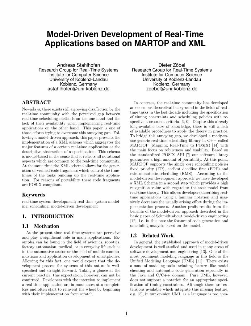
ABSTRACTNowadays, there exists still a growing disaffection by thereal-time community with the perceived gap betweenreal-time scheduling methods on the one hand and thelack of their availability when implementing real-timeapplications on the other hand. This paper is one ofthose efforts trying to overcome this annoying gap. Fol-lowing a model-driven approach, this paper presents theimplementation of a XML schema which aggregates themajor features of a certain real-time application at thedescriptive abstraction of a specification. This schemais model-based in the sense that it reflects all notationalaspects which are common to the real-time community.At the same time the XML schema allows for the gener-ation of verified code fragments which control the time-liness of the tasks building up the real-time applica-tion. For reasons of portability these code fragmentsare POSIX-compliant.
Keywordsreal-time system development; real-time system model-ing; scheduling; model-driven development
1. INTRODUCTION
1.1 MotivationAt the present time real-time systems are pervasive
and play a significant role in many applications. Ex-amples can be found in the field of avionics, robotics,factory automation, medical, or in everyday life such asin the automotive sector or the field of mobile commu-nications and application development of smartphones.Allowing for this fact, one would expect that the de-velopment process for systems of this nature is well-specified and straight forward. Taking a glance at thecurrent practice, this expectation, however, can not beconfirmed. Developers with the intention to implementa real-time application are in most cases at a completeloss and often start to reinvent the wheel by beginningwith their implementation from scratch.
In contrast, the real-time community has developedan enormous theoretical background in the fields of real-time tasks in the last decade including the specificationof timing constraints and scheduling policies with re-spective assessment criteria [6, 9]. Despite this alreadylong-available base of knowledge, there is still a lackof available procedures to apply the theory in practice.To bridge this annoying gap, we developed a ready-to-use generic real-time scheduling library in C++ calledMARTOP (Mapping Real-Time to POSIX) [14] withthe main focus on robustness and usability. Based onthe standardized POSIX API [7] our software libraryguarantees a high amount of portability. At this point,MARTOP supports the single core scheduling policiesfixed priority (FP), earliest deadline first (EDF) andrate monotonic scheduling (RMS). According to themodel-driven development approach we have developeda XML Schema in a second step which provides a highrecognition value with regard to the task model fromreal-time theory. This allows developers describing real-time applications using a familiar notation and mas-sively decreases the usually arising effort during the im-plementation process. Another profit results from thebenefits of the model-driven approach described in thebasic paper of Schmidt about model-driven engineering[12], i.e. in this case the feature of code generation andscheduling analysis based on the model.
1.2 Related WorkIn general, the established approach of model-driven
development is well-studied and used in many areas ofsoftware development and engineering [13]. One of themost prominent modeling language in this field is theUnified Modeling Language (UML) [11]. There existsa mass of modeling tools including features like modelchecking and automatic code generation especially inthe Java and C/C++ domain. Pure UML, however,does not support a notation for an appropriate speci-fication of timing constraints. Although there are ex-tensions available which integrate this missing feature,e.g. [5], in our opinion UML as a language is too com-
1

plex and does not reflect the models and notations fromthe real-time theory. Available studies also show thatUML is hardly used in many software companies [10, 1].A more intuitive way for specifying particularly timingconstraints and scheduling policy of a real-time appli-cation is necessary.
Another alternative to model the timing constraintsof a real-time application is based on timed automataand was first introduced by Alur and Dill in [2]. Themain goal of this approach is the verification of the sys-tem behaviour according to a given specification andbased on model-checking algorithm from the field offormal methods. A common tool with graphical userinterface is UPPAAL [8] which can be used for mod-eling and verifying real-time application specificationsbased on timed automata[4]. But the modeling processis a complex task and requires a great knowledge in thefield of formal methods and reachability analysis. Thus,this approach yields no benefit for our purpose becausewe want to provide a familiar notation in accordance toreal-time theory.
1.3 Outline of this paperThe remainder of this paper is organized as follows.
In section 2.1 we describe the underlying task modeland the necessary notations which are important forunderstanding the rest of the paper. Chapter 2.2 intro-duces an example application which is used to describeour model-driven approach. The XML schema to modelreal-time applications is described in chapter 2.3. Thefeatures of scheduling analysis and code generation areintroduced in chapters 2.4 and 2.5. Finally, the resultsof our work are discussed in chapter 3 and an outlookto planned future work is given.
2. MODEL-DRIVEN APPROACHThe overall process of the presented model-driven ap-
proach is illustrated in Figure 1 and is divided into anintellectual and a semi-automated process. The intel-lectual part is the one where the developer has to lenda hand whereas the semi-automated process is tool-supported. The core component is the XML specifi-cation according to a respective XML schema.
2.1 Task model and notationsThe following assumes a set T of independent peri-
odic preemptive tasks which are scheduled on a singlecore CPU. A given task τi is specified by a tuple of theform (Ci, Ti, Ai, Di) where Ci is the worst case execu-tion time, Ti the rate, Ai the relative arrival time andDi the relative deadline of the task.
A schedule for a given set of tasks T is a functionN→ T which assigns for each time unit an active task.The schedule repeats after a duration LT ∈ N accordingto all scheduled tasks T with
LT = lcm (T1, ..., Tn) . (1)
theory-based design of a real-
time application
XML application
specification
verified generation of
POSIX-based C++ code
scheduling analysis
semi-automated processintellectual process
Figure 1: Conceptual illustration of the model-based development of real-time systems usingthe presented XML schema.
The schedule is feasible if for the duration of LT notask τi ∈ T invalidates its relative deadline Di for itscurrent execution. Furthermore, it is possible to assigna priority pi ∈ N to a task τi ∈ T . At each clockcycle of a schedule the task with the highest priority isexecuted. The priority value assigned to a task dependson the used scheduling policy.
2.2 Example application: Ball on a platesystem
As an example application we use a ball on a platesystem. The goal of such a system is balancing a ballin the center of a plate which is controlled in a two-dimensional manner using a stepping motor for eachaxis. A webcam is mounted vertically above the plateto capture the ball position. Overall, we can divide thesystem into three main tasks:
1. Capturing the ball position using the webcam.
2. A calculation component which is divided in thefollowing subtasks:
(a) Image processing algorithm to calculate theexact ball position.
(b) Calculating the manipulated value for the step-ping motors using a PID controller.
(c) Sending the value to the stepping motors.
3. Sending diagnostic information via UDP port.
Although the calculation component comprises threesubtasks, they are executed as one task due to theirstrong sequential nature. The three main tasks arescheduled using EDF as scheduling policy. This ensuresthat a new image can be captured while the previousone is processed. Diagnostic informations, e.g. the cur-rent ball position, are sent asynchronously via UDP toa specified remote computer. The timing constraintsincluding the wcet and the rate are illustrated in table1. The wcet of a single task was determined empiricalby executing a set of test runs.
2
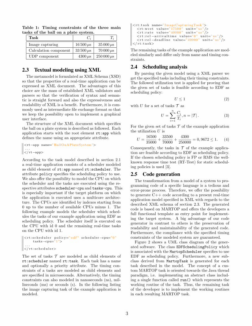
Table 1: Timing constraints of the three maintasks of the ball on a plate system.
Task Ci Ti
Image capturing 16 500µs 35 000µs
Calculation component 33 500µs 70 000µs
UDP component 4300µs 250 000µs
2.3 Textual modeling using XMLThe metamodel is formulated as XML Schema (XSD)
so that the properties of a real-time application can beexpressed as XML document. The advantages of thischoice are the mass of established XML validators andparsers so that the verification of syntax and seman-tic is straight forward and also the expressiveness andreadability of XML is a benefit. Furthermore, it is com-monly used as intermediate file exchange format so thatwe keep the possibility open to implement a graphicaluser interface.
The structure of the XML document which specifiesthe ball on a plate system is described as followed. Eachapplication starts with the root element rt:app whichdefines the name using an appropriate attribute.
<rt−app name=”BallOnAPlateSystem ”>. . .</ rt−app>
According to the task model described in section 2.1a real-time application consists of a scheduler modeledas child element of rt:app named rt:scheduler. Theattribute policy specifies the scheduling policy to use.We also offer the possibility to model the CPU on whichthe scheduler and the tasks are executed using the re-spective attributes scheduler-cpu and tasks-cpu. Thisis especially important if the target platform on whichthe application is executed uses a multicore architec-ture. The CPUs are identified by indexes starting from0 up to the number of available CPUs minus 1. Thefollowing example models the scheduler which sched-ules the tasks of our example application using EDF asscheduling policy. The scheduler itself is executed onthe CPU with id 0 and the remaining real-time taskson the CPU with id 1.
<r t : s c h e d u l e r po l i c y=”edf ” scheduler−cpu=”0 ”tasks−cpu=”1 ”>
. . .</ r t : s c h e d u l e r>
The set of tasks T are modeled as child elements ofrt:scheduler named rt:task. Each task has a nameand optionally a priority attribute. The timing con-straints of a tasks are modeled as child elements andare specified in microseconds. Alternatively, the timingconstraints can also modeled in nanoseconds (ns), mil-liseconds (ms) or seconds (s). In the following listingthe image capturing task of the example application ismodeled.
<r t : t a s k name=”ImageCapturingTask ”><r t :wc e t value=”17500 ” un i t=”us ”/>< r t : r a t e va lue=”40000 ” un i t=”us ”/>< r t : r e l −a r r i v a l t ime value=”0 ” un i t=”us ”/>< r t : r e l −dead l ine va lue=”40000 ” un i t=”us ”/>
</ r t : t a s k>
The remaining tasks of the example application are mod-eled similarly and differ only from name and timing con-straints.
2.4 Scheduling analysisBy parsing the given model using a XML parser we
get the specified tasks including their timing constraints.The followed utilization test is applied for proving thatthe given set of tasks is feasible according to EDF asscheduling policy:
U ≤ 1 (2)
with U for a set of tasks T as
U =n∑
i=1
Ci
Ti, n = |T | . (3)
For the given set of tasks T of the example applicationthe utilization U is
U =16500
35000+
33500
70000+
4300
250000= 0, 9672 ≤ 1. (4)
Consequently, the tasks in T of the example applica-tion are feasible according to EDF as scheduling policy.If the chosen scheduling policy is FP or RMS the well-known response time test (RT-Test) for static schedul-ing policies is used [3].
2.5 Code generationThe transformation from a model of a system to pro-
gramming code of a specific language is a tedious anderror-prone process. Therefore, we offer the possibilityto generate C++ code according to a present real-timeapplication model specified in XML with regards to thedescribed XML schema of section 2.3. The generatedcode is based on MARTOP and offers the developers afull functional template as entry point for implement-ing the target system. A big advantage of our codegenerator in contrast to others is the preservation ofreadability and maintainability of the generated code.Furthermore, the compliance with the specified timingconstraints of the modeled system are guaranteed.
Figure 2 shows a UML class diagram of the gener-ated software. The class EDFSchedulingPolicy whichis associated with the MartopScheduler specifies to useEDF as scheduling policy. Furthermore, a new sub-class derived from MartopTask is generated for eachtask described in the model. The concept of a cus-tom MARTOP task is oriented towards the Java threadparadigm, i.e. implementing an abstract class includ-ing a single function called run() which represents theworking routine of the task. Thus, the remaining taskof the developer is to implement the working routinesin each resulting MARTOP task.
3

Figure 2: UML class diagram for demonstrating the structure and resulting classes which are gener-ated based on the MARTOP library.
3. CONCLUSION AND FUTURE WORKIn this paper we presented an approach to model the
software part of a real-time application using XML. Thestructure of the XML document is described via a XMLschema and can be appropriately validated. The result-ing XML structure is based on the task model from thereal-time theory and offers developers an intuitive pos-sibility for describing scheduling policy and timing con-straints of a real-time application. With the help of anexample application the features of scheduling analysisand code generation are presented.
The aim of our work is to support real-time appli-cation developers and make their life easier. In ouropinion, a step in the right direction has been madewith the approach presented in this paper. But thereare still lacking features. First, we assume a single-coreprocessor but multi-core processors are already stateof the art. Accordingly, a future development in thedirection of multi-core scheduling is urgent and neces-sary. Second, the modeling capabilities are kept simpleand the full advantage of this approach is not taken.On the one hand, this fact makes it easy for develop-ers to learn how to model a real-time application usingour approach. On the other hand, it is only possible tomodel applications with low complexity that makes ourapproach for most real-world applications insufficientat this time. Our major request is to offer our softwareand tools to other developers and support them in de-veloping real-time applications, so these future workswill make our approach applicable for the practice.
4. REFERENCES[1] L. T. W. Agner, I. W. Soares, P. C. Stadzisz, and
J. M. SimaO. A Brazilian survey on UML andmodel-driven practices for embedded softwaredevelopment. J. Syst. Softw., 86(4):997–1005,2013.
[2] R. Alur and D. L. Dill. Automata for modelingreal-time systems. In Proc. seventeenth Int.Colloq. Autom. Program., pages 322–335.Springer, 1990.
[3] N. Audsley, A. Burns, M. Richardson, K. Tindell,and A. J. Wellings. Applying new scheduling
theory to static priority pre-emptive scheduling.Softw. Eng. J., 8(5):284–292, 1993.
[4] J. Bengtsson, K. G. Larsen, F. Larsson,P. Pettersson, and W. Yi. Uppaal — a Tool Suitefor Automatic Verification of Real–Time Systems.Work. Verif. Control Hybrid Syst. III,(1066):232–243, 1995.
[5] S. Burmester, H. Giese, and W. Schafer.Model-driven architecture for hard real-timesystems: From platform independent models tocode. In Eur. Conf. Model Driven Archit. Appl.,pages 25–40. Springer, 2005.
[6] G. Buttazzo. Hard Real-Time ComputingSystems: Predictable Scheduling Algorithms andApplications. Springer, 2011.
[7] ISO/IEC 9945-1. Information Technology -Portable Operating System Interface (POSIX) -Part 1: System Application Program Interface(API) [C Language]. Technical report, Institute ofElectrical and Electronic Engineers (IEEE), 1996.
[8] K. Larsen, P. Pettersson, and W. Yi. UPPAAL ina nutshell. Int. J. Softw. Tools . . . , pages134–152, 1997.
[9] F. Liu, A. Narayanan, and Q. Bai. Real-timesystems. 2000.
[10] M. Petre. UML in practice. In Proc. 2013 Int.Conf. Softw. Eng., pages 722–731. IEEE Press,2013.
[11] J. Rumbaugh, I. Jacobson, and G. Booch. UnifiedModeling Language Reference Manual. PearsonHigher Education, 2004.
[12] D. Schmidt. Guest Editor’s Introduction:Model-Driven Engineering. Computer (Long.Beach. Calif)., 39(2):25–31, 2006.
[13] D. C. Schmidt. Model-driven engineering. IEEEComput., 39(2):25–31, 2006.
[14] A. Stahlhofen and D. Zobel. Mapping Real-Timeto POSIX. In R. Stojanovic, L. Jozwiak, andD. Jurisic, editors, 4th Mediterr. Conf. Embed.Comput., pages 89–92, Budva, Montenegro, 2015.
4

Model Checking of Cache for WCET Analysis Refinement
Valentin TouzeauUniv. Grenoble Alpes
CNRS, VERIMAG, F-38000Grenoble, France
Claire MaïzaUniv. Grenoble Alpes
CNRS, VERIMAG, F-38000Grenoble, France
David MonniauxUniv. Grenoble Alpes
CNRS, VERIMAG, F-38000Grenoble, France
ABSTRACTOn real-time systems running under timing constraints,scheduling can be performed when one is aware of theworst case execution time (WCET) of tasks. Usually, theWCET of a task is unknown and schedulers make use ofsafe over-approximations given by static WCET analysis.To reduce the over-approximation, WCET analysis has togain information about the underlying hardware behavior,such as pipelines and caches. In this paper, we focus on thecache analysis, which classifies memory accesses ashits/misses according to the set of possible cache states.We propose to refine the results of classical cache analysisusing a model checker, introducing a new cache model forthe least recently used (LRU) policy.
KeywordsWorst Case Execution Time, Cache Analysis, ModelChecking, Least Recently Used Cache
1. INTRODUCTIONOn critical systems, one should be able to guarantee that
each task will meet its deadline. This strong constraint canbe satisfied when the scheduler has bounds on every tasks’execution time. The aim of a WCET analysis is to computesuch safe bounds statically. In order to provide a satisfiablebound, the WCET analysis needs to model the execution ofinstructions at the hardware level. However, to avoid thehuge latency of main memory access, one can copy partsof the main memory into small but fast memories calledcaches. In order to retrieve precise bounds on the executiontime of instructions, it is thus mandatory to know whichinstructions are in the cache and which are not. In thispaper we focus on instruction caches, ie. we aim at knowingwhether instructions of the program are in the cache whenthey are executed.
For efficiency reasons, the main memory is partitionedinto fixed size blocks. To avoid repeated accesses to thesame block, they are temporary copied into the cache whenrequested by the CPU. This way, they can be retrieved fasteron the next access, without requesting the main memoryagain. Moreover, to speed up the retrieval of blocks fromthe cache, caches are usually partitioned into sets of equalsizes. A memory block can only be stored in one set thatis uniquely determined by the address of the block. Thus,when searching a block in the cache, it is looked for in onlyone set. Since the main memory is bigger than the cache, itmay happen that a set is already full when trying to store
a new block in it. In this case, one block of the set hasto be evicted in order to store the new one. This choicedoes not depend on the content of the other sets and is doneaccording to the cache replacement policy. In our case, wefocus on the Least Recently Used (LRU) policy (for otherpolicies, refer to [5]). A cache set using the LRU policy canbe represented as a queue containing blocks ordered fromthe most recently accessed (or used) to the least recentlyaccessed. When the CPU requests a block that is not inthe cache (cache miss), it is stored at the beginning of thequeue (it becomes the most recently used block) and thelast block (the least recently used) is evicted. On the otherhand, when the requested block is already in the cache, it ismoved to the beginning of the queue, delaying its eviction.The position of a block in the queue is called the age of theblock: the youngest block is the most recently used and theoldest is the least recently used.
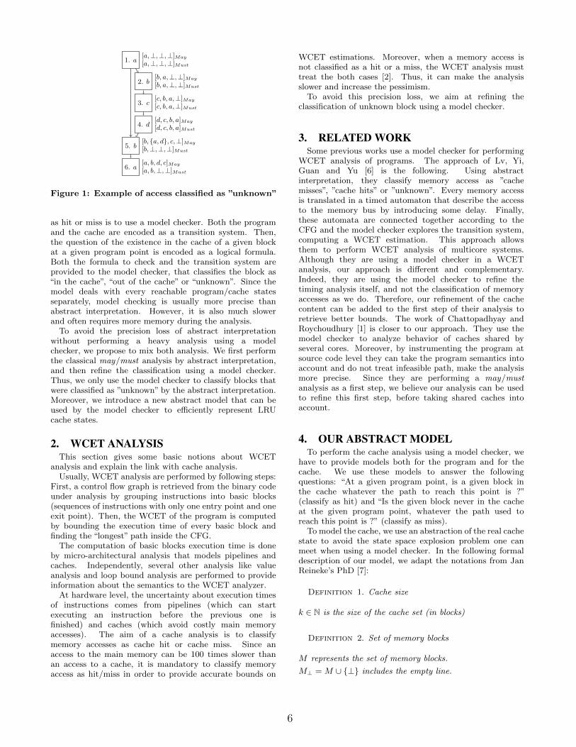
The aim of a cache analysis is to provide a classificationof memory accesses as ”cache hit”, ”cache miss” or”unknown” (not always a hit, and not always a miss) to beused as part of the WCET analysis. This classification isusually established by abstract interpretations called ”MayAnalysis” and ”Must Analysis” that respectively compute alower and upper bound of every block’s age. For moredetails about these analysis, refer to [3]. Must analysis isused to predict the cache hits (if a block must be in thecache when accessing it, access is a hit), whereas mayanalysis is used to predict the misses (if a block may not bein the cache when accessing it, access is a miss). However,if a block is in the may cache but not in the must cache, itis classified as unknown. This can happen because thisaccess is sometimes a miss and sometimes a hit, or becausethe abstract interpretation is too coarse. An example isgiven on Figure 1. Program states (basic blocks) are on theleft, whereas abstract cache states (may and must) at theexit of basic blocks are on the right. For simplicity, everybasic block is stored in exactly one memory block. Forexample, at the exit of block 5, the minimum age of blocksa, b, c and d computed by the may analysis are respectively1, 0, 2 and 1. At block 6, a is accessed and is in the cache(because there are only 4 different blocks, and they all fittogether in the cache), thus it should be classified as a hit.However, it is classified as ”unknown” by the may and mustanalysis because of an over-approximation performed bythe must analysis. Indeed, at entry of block 5, the mustcache is [⊥,⊥,⊥, a] because a is the only block that mustbe accessed, and b, c and d may be accessed since the lastaccess to a. An other possibility to classify memory access
5
1. a
2. b
3. c
4. d
5. b
6. a
[a,⊥,⊥,⊥]May
[a,⊥,⊥,⊥]Must
[b, a,⊥,⊥]May
[b, a,⊥,⊥]Must
[c, b, a,⊥]May
[c, b, a,⊥]Must
[d, c, b, a]May
[d, c, b, a]Must
[b, {a, d}, c,⊥]May
[b,⊥,⊥,⊥]Must
[a, b, d, c]May
[a, b,⊥,⊥]Must
Figure 1: Example of access classified as ”unknown”
as hit or miss is to use a model checker. Both the programand the cache are encoded as a transition system. Then,the question of the existence in the cache of a given blockat a given program point is encoded as a logical formula.Both the formula to check and the transition system areprovided to the model checker, that classifies the block as“in the cache”, “out of the cache” or “unknown”. Since themodel deals with every reachable program/cache statesseparately, model checking is usually more precise thanabstract interpretation. However, it is also much slowerand often requires more memory during the analysis.
To avoid the precision loss of abstract interpretationwithout performing a heavy analysis using a modelchecker, we propose to mix both analysis. We first performthe classical may/must analysis by abstract interpretation,and then refine the classification using a model checker.Thus, we only use the model checker to classify blocks thatwere classified as ”unknown” by the abstract interpretation.Moreover, we introduce a new abstract model that can beused by the model checker to efficiently represent LRUcache states.
2. WCET ANALYSISThis section gives some basic notions about WCET
analysis and explain the link with cache analysis.Usually, WCET analysis are performed by following steps:
First, a control flow graph is retrieved from the binary codeunder analysis by grouping instructions into basic blocks(sequences of instructions with only one entry point and oneexit point). Then, the WCET of the program is computedby bounding the execution time of every basic block andfinding the “longest” path inside the CFG.
The computation of basic blocks execution time is doneby micro-architectural analysis that models pipelines andcaches. Independently, several other analysis like valueanalysis and loop bound analysis are performed to provideinformation about the semantics to the WCET analyzer.
At hardware level, the uncertainty about execution timesof instructions comes from pipelines (which can startexecuting an instruction before the previous one isfinished) and caches (which avoid costly main memoryaccesses). The aim of a cache analysis is to classifymemory accesses as cache hit or cache miss. Since anaccess to the main memory can be 100 times slower thanan access to a cache, it is mandatory to classify memoryaccess as hit/miss in order to provide accurate bounds on
WCET estimations. Moreover, when a memory access isnot classified as a hit or a miss, the WCET analysis musttreat the both cases [2]. Thus, it can make the analysisslower and increase the pessimism.
To avoid this precision loss, we aim at refining theclassification of unknown block using a model checker.
3. RELATED WORKSome previous works use a model checker for performing
WCET analysis of programs. The approach of Lv, Yi,Guan and Yu [6] is the following. Using abstractinterpretation, they classify memory access as ”cachemisses”, ”cache hits” or ”unknown”. Every memory accessis translated in a timed automaton that describe the accessto the memory bus by introducing some delay. Finally,these automata are connected together according to theCFG and the model checker explores the transition system,computing a WCET estimation. This approach allowsthem to perform WCET analysis of multicore systems.Although they are using a model checker in a WCETanalysis, our approach is different and complementary.Indeed, they are using the model checker to refine thetiming analysis itself, and not the classification of memoryaccesses as we do. Therefore, our refinement of the cachecontent can be added to the first step of their analysis toretrieve better bounds. The work of Chattopadhyay andRoychoudhury [1] is closer to our approach. They use themodel checker to analyze behavior of caches shared byseveral cores. Moreover, by instrumenting the program atsource code level they can take the program semantics intoaccount and do not treat infeasible path, make the analysismore precise. Since they are performing a may/mustanalysis as a first step, we believe our analysis can be usedto refine this first step, before taking shared caches intoaccount.
4. OUR ABSTRACT MODELTo perform the cache analysis using a model checker, we
have to provide models both for the program and for thecache. We use these models to answer the followingquestions: “At a given program point, is a given block inthe cache whatever the path to reach this point is ?”(classify as hit) and “Is the given block never in the cacheat the given program point, whatever the path used toreach this point is ?” (classify as miss).
To model the cache, we use an abstraction of the real cachestate to avoid the state space explosion problem one canmeet when using a model checker. In the following formaldescription of our model, we adapt the notations from JanReineke’s PhD [7]:
Definition 1. Cache size
k ∈ N is the size of the cache set (in blocks)
Definition 2. Set of memory blocks
M represents the set of memory blocks.
M⊥ = M ∪ {⊥} includes the empty line.
6

Definition 3. Set of Cache States
CLRU ⊂Mk⊥ symbolizes the set of reachable cache states
[b1, b2, . . . , bk] ∈ CLRU represents a reachable state
b1 is the least recently used block
In addition of these notation, to define our abstract model,we introduce the following notations: A, represents the setof abstract cache states, εa ∈ A, represents cache statesthat does not contain a, and [S]a ∈ A, represents cachestates that contains a and some other blocks younger thana (forming the set S), where a ∈M is a memory block.
Definition 4. Set of Abstract Cache States
A = P(CLRU ) is the power set of reachable cache states.
Definition 5. Abstract Cache States
εa ={
[b1, ..., bk] ∈ CLRU ,∀i ∈ J1, kK, bi 6= a}∈ A
[S]a ={
[b1, ..., bk] ∈ CLRU ,
∃i ∈ J1, kK, bi = a ∧ (bj ∈ S ⇔ j < i)}∈ A
The idea behind the abstract model we define below is totrack only one block (noted a). Indeed, to know whether ablock is in a LRU cache, you only have to count the numberof accesses made to pairwise different blocks since the lastaccess to it. In other words, you do not have to know the ageof others blocks, you are only interested in knowing if theyare younger than the block you are tracking. Therefore, wegroup together cache states that have the same set of blocksyounger than the block we want to track.
To every cache state p, we associate an abstract stateαa(p) which consists of the set of values younger than a inthe cache or a special value in the case where a is not inthe cache.
Definition 6. Abstraction of Cache States
αa : CLRU → A
αa ([b1, ..., bk]) =
{εa if ∀i ∈ J1, kK, bi 6= a
[{b1, ..., bi−1}]a if ∃i ∈ J1, kK, bi = a
For example, when tracking block a, the abstract cachestate associated to the exit of block 1 of Figure 1 is [{}]a,symbolizing that a is the least recently used block at thispoint (the set of younger blocks is empty). At the exit ofblock 4, the abstract cache state is [{b, c, d}]a.
Additionally, we define the partial function updateaLRU(k),which models the effect of accessing a block on an abstractstate. When the abstract cache state does not contain a (i.e.is equal to εa), it remains unchanged until an access to a ismade. When a is accessed, every new block access appearsinto the set S. When the cardinal of S reaches k−1 (a is theleast recently used block), a new access to a different blockevicts a (and new abstract cache state is reset to εa). If anaccess to a is done in the meantime, the set S of youngerblock is reset to {}.
Definition 7. Abstract State Update
updateaLRU(k) : A×M → A
updateaLRU(k)(εa, c) =
{[{}]a if a = c
εa if a 6= c
updateaLRU(k)([S]a, c) =[{}]a if c = a
[S]a if c 6= a and c ∈ S[S ∪ {c}]a if c 6= a and c /∈ S and |S| < k − 1
εa if c 6= a and c /∈ S and |S| = k − 1
Considering the example of Figure 1, the model checkerassociates two different abstract states to block 5 dependingon the incoming flow from block 1 or block 4. These statesare respectively [{}]a and [{b, c, d}]a. Thus, applying theupdate function for treating the access made to b in block 5,we obtain [{b}]a and [{b, c, d}]a. Therefore, we know that ais not evicted from the cache by block 5 and access made toa in block 6 is not classified as unknown anymore but as ahit.
The second part of our model is the model of theprogram. Since we focus on instruction caches, the modelwe use for the program is a graph obtained from the CFGby splitting basic blocks (when needed) into blocks of thesize of a memory block. Thus, a path in the modelrepresents the sequence of memory access that theinstruction cache handles during the execution of theprogram. However, because we only track one memoryblock at a time, it is also possible to simplify the controlflow graph according to this block. Indeed, one can slicethe CFG according to the cache set associated to the blockwe want to track, removing every memory access to another cache set. Moreover, we can remove from theobtained graph every node that is not an access to a andthat does not contribute to a eviction. Thus, it appearsthat every node that does not contain a in their entry maycache can be removed.
[. . . ]a
εa
[. . . ]a
access to a
eviction of a
Figure 2: Simplifying CFG according to access to a
This simplification of the CFG is illustrated on figure 2.Plain arrows represent program flow potentiallymanipulating block a, whereas dashed arrows representflow that does not and that can be simplified in only onearrow. At some point after an access to block a, we can besure that a is not in the cache anymore. Therefore, it ispossible to remove all nodes (dashed arrows) from thispoint until the next access to a.
5. IMPLEMENTATION / EXPERIMENTSThis section describe the prototype we build and the
experiments we made to valid our proof of concept. Theworkflow of our analysis is illustrated on Figure 3.
Our implementation does not use directly the binarycode to analyze but runs on the LLVM bytecoderepresentation of it. We first build the CFG of the programfrom the bytecode using the LLVM framework. Since the
7

Program Size4 ways 8 ways 16 ways
Un Nc Un Nc Un Ncrecursion 26 34.6% 11.1% 53.8% 7.1% 53.8% 21.4%
fac 26 34.6% 11.1% 46.1% 8.3% 46.1% 41.6%binarysearch 48 12.5% 0% 56.2% 29.6% 52.0% 12.0%
prime 57 10.5% 0% 29.8% 35.2% 57.8% 18.1%insertsort 58 23.7% 28.5% 28.8% 11.7% 55.9% 9.0%
bsort 62 30.6% 57.8% 53.2% 6.0% 62.9% 5.1%duff 64 10.9% 0% 37.5% 12.5% 37.5% 12.5%
countnegative 65 21.5% 21.4% 43.0% 21.4% 52.3% 20.5%st 137 14.5% 30.0% 43.7% 13.3% 69.3% 5.2%
ludcmp 179 11.1% 5.0% 39.6% 15.4% 67.5% 4.1%minver 265 20.7% 29.0% 44.1% 12.8% 63.0% 10.7%
statemate 582 7.5% 2.2% 7.9% 4.3% 8.2% 2.0%
Table 1: Precision of May/Must analysis and Model Checker
CFGCache
Configuration
Hit/MissClassification
May/MustAnalysis
CacheModeling
ModelChecker
Unknown
Not unknown
Figure 3: Workflow of our prototype
LLVM bytecode does not affect any address toinstructions, we have to provide a mapping of instructionsto the main memory. For our prototype, we assume thatevery instruction has the same size in memory. Thus,memory blocks contain a fixed number of instructions andcan be obtain by splitting basic blocks of the CFG intofixed size blocks. Using this mapping and the CFG, ourprototype performs a may/must analysis of the program.For every block access classified as unknown, we build anabstract model of the cache and provide it to the modelchecker together with the CFG (simplified as explainabove). It would be possible to use real addresses frombinary code and a correspondence between LLVM bytecodeand binary code, as done in [4], but this requires significantengineering and falls outside of the scope of thisexperiment.
We experiment our prototype with benchmarks of theTacleBench1. Table 1 contains the results of ourexperiments. Size of program is given in number ofmemory block. We run our experiments with caches ofonly one cache set, with different sizes: 4, 8 or 16 ways.For every experiment, we measure both the amount ofaccesses classified as “unknown” by the may/must analysis(column “Un”) and the amount of accesses newly classifiedas “always in the cache” or “always out of the cache” amongthe accesses left “unknown” by the may/must analysis(column Nc). During these experiments, our analysisclassifies up to 57.8% of the accesses left unclassified by theabstract interpretation analysis.
6. CONCLUSIONWe proposed to refine classical cache analysis by using
a model checker. To avoid the common problem of statespace explosion meet when dealing with model checking, weintroduce a new abstract cache model. This model allows
1http://www.tacle.eu/index.php/activities/taclebench
us to compute the exact age of a memory block along anexecution path of the program. Thus, we can select thememory block we want to refine. Moreover, it allows usto simplify the program model too, by removing some nodesuseless to the refinement. Finally, we implement a prototypeand test it on a benchmark. Our experiments shows that ourapproach is able to refine up to 60% of the memory accessclassified as unknown by the abstract interpretation.
Our prototype runs on LLVM bytecode, and use anunrealistic memory mapping. As future work, we aim atimplementing an analyzer that runs on the binary code. Tofinally validate our approach, it is also possible to comparethe performance of our analysis to other analysis refiningmay/must analysis, like persistence analysis or analysisperforming virtual inlining and unrolling.
7. REFERENCES[1] S. Chattopadhyay and A. Roychoudhury. Scalable and
precise refinement of cache timing analysis via modelchecking. In RTSS 2011. IEEE Computer Society, 2011.
[2] C. Cullmann, C. Ferdinand, G. Gebhard, D. Grund,C. Maiza, J. Reineke, B. Triquet, and R. Wilhelm.Predictability considerations in the design of multi-coreembedded systems.
[3] C. Ferdinand. Cache behavior prediction for real-timesystems. Pirrot, 1997.
[4] J. Henry, M. Asavoae, D. Monniaux, and C. Maiza.How to compute worst-case execution time byoptimization modulo theory and a clever encoding ofprogram semantics. In Y. Zhang and P. Kulkarni,editors, SIGPLAN/SIGBED, LCTES ’14. ACM, 2014.
[5] M. Lv, N. Guan, J. Reineke, R. Wilhelm, and W. Yi. Asurvey on static cache analysis for real-time systems.LITES, 2016.
[6] M. Lv, W. Yi, N. Guan, and G. Yu. Combiningabstract interpretation with model checking for timinganalysis of multicore software. In RTSS2010, pages339–349. IEEE Computer Society, 2010.
[7] J. Reineke. Caches in WCET Analysis: Predictability -Competitiveness - Sensitivity. PhD thesis, SaarlandUniversity, 2009.
8

On Scheduling Sporadic Non-Preemptive Tasks withArbitrary Deadline using Non-Work-Conserving
Scheduling
Homa IzadiIslamic Azad University, E-Campus,
Tehran, [email protected]
Mitra NasriMax Planck Institute for Software Systems,
Kaiserslautern, [email protected]
ABSTRACTIn this paper, we consider the problem of scheduling a setof non-preemptive sporadic tasks with arbitrary deadlineson a uni-processor system. We modify the Precautious-RMalgorithm which is an online non-preemptive scheduling al-gorithm based on rate monotonic priorities to cope with ar-bitrary deadlines and sporadic releases. Our solution is anO(1) non-work-conserving scheduling algorithm.
1. INTRODUCTIONNon-preemptive scheduling reduces both run-time and de-
sign time overheads. At run-time, it avoids context switches,and hence, preserves the state of the cache and CPU pipelinesfor the task. At design-time, it simplifies the required mech-anisms for guaranteeing mutual exclusion. Besides, due tothese properties, it improves the accuracy of estimating theworst-case execution-time (WCET) of a task. Thus, it allowssystem designers to have a more realistic and less pessimisticconfiguration setup for the system.
Moreover, non-preemptive execution improves the qualityof service in control systems because it efficiently reducesthe delay between sampling and actuation [9]. By doing so,it increases the freshness of a sampled data. In a preemptivesystem, if a task is preempted after reading its data from theenvironment (and before using that data), the data becomesold, and hence, after resuming, the task uses the old data tocalculate the output command. Consequently, controller’saccuracy may reduce.
In the non-preemptive scheduling, a processing resource(or other resources) can be blocked for a long time, caus-ing a timing violation for the tasks with shorter deadlines.Thus, in a feasible task set, the maximum execution timeof a task is restricted. Cai et al., [1] have shown that in aperiodic task set, the maximum permissible execution timeof the tasks except τ1 (the task with the smallest period),is at most 2(T1 − C1) (where T1 and C1 are the period andWCET of τ1). For example, if the smallest period is 1ms andthe largest period is 1000ms (which is regularly the case forthe runnables in the automotive industry), then the largestexecution time cannot be greater than 2ms. It means thatthose tasks with large period must be heavily under-utilized,otherwise, the system will not be schedulable.
In order to cope with the limitation of non-preemptivescheduling, many researches have focused on finding a safespeed-up factor, using which no task will miss its dead-line (under a particular scheduling algorithm such as non-preemptive rate monotonic (NP-RM), or non-preemptiveEDF (NP-EDF) [8]). However, as shown in [3], this speed-up factor may become an unreasonably large number (e.g.,
120). Such a speed-up factor may not be useful for a real sys-tem where the weight, size, power consumption, and manyother factors affect the choice of processor.
In many real-time systems (e.g., control or multimediasystems), finishing a task after its deadline will not causea failure for the system (the system might not even be asafety-critical system to begin with). For example, in con-trol systems, usually the stability of the controller will notbe affected if one of the samples is taken later than theexpected sampling period [9]. Such event may affect thequality of control, however, it may probably not affect thestability of the controller as long as the completion timeis within a certain deadline. In other words, deadlines arenot necessarily smaller than or equal to periods. As a result,the tasks can tolerate longer blocking time caused by a lowerpriority task. It allows us to have a non-preemptive systemwith longer execution times than one mentioned previously.
Recently, there have been some advancements in the stateof non-work-conserving scheduling algorithms [4,5,7]. Thesealgorithms may leave the processor idle even if there arepending jobs in the system. The idea of these works is toadd an idle-time insertion policy (IIP) to the existing jobscheduling policies such as RM and EDF to increase schedu-lability. The role of the job scheduling policy is to select ajob with the highest priority, and the role of IIP is to decidewhether to schedule that job or instead, to leave the proces-sor idle. It has been shown [5] that by adding an IIP to thejob scheduling policy, a significant number of task sets thatare not schedulable by the job scheduling policy itself (e.g.,RM and EDF) become schedulable if an idle-time insertionpolicy is used.
In our work, we focus on the problem of scheduling non-preemptive sporadic tasks with arbitrary deadlines upon auni-processor system. We use the Precautious-RM (P-RM)from [7] as the basis of our algorithm, and modify it in threeways: 1) we increase its eagerness to schedule tasks ratherthan scheduling idle intervals, 2) we replace the existing IIPwith the one which is based on arbitrary deadlines ratherthan implicit deadlines, and 3) we add mechanisms for en-abling it to schedule sporadic tasks. Then we discuss how aschedulability test can be developed for the new algorithm.Our final solution is an online non-preemptive schedulingalgorithm, called AD-PRM (where AD stands for arbitrarydeadline). It has O(1) computational complexity per acti-vation of the if the number of priorities in the system is areasonable constant number.
In the rest of the paper we describe system model inSect. 2. The AD-PRM, is presented in Sect. 3. Open chal-lenges and future work are presented in Sect. 4. Sect. 5presents the experimental results. In Sect. 4 we discuss
9

Figure 1: Examples of P-RM schedules in compari-son with an optimal schedule.
about future work and then conclude the paper in Sect. 6.
2. SYSTEM MODEL AND BACKGROUNDWe consider a set of independent, non-preemptive spo-
radic tasks, with arbitrary deadlines which must be sched-uled on a single processor. Task set τ = {τ1, τ2, . . . , τn} hasn tasks and each task is identified by τi : (Ci, Ti, Di), whereCi is the worst-case execution time (WCET), Ti is the period(the minimum inter-arrival time), and Di is the deadline ofthe task. We assume Ci, Ti, and Di are integer multiples ofthe system’s clock, thus they are integer values. We denotesystem utilization by U =
∑ni=1 ui where ui = Ci/Ti is the
utilization of task τi. The hyperperiod is the least commonmultiple of the periods. Tasks are indexed according to theirperiod so that T1 < T2 ≤ . . . ≤ Tn.
Next, we explain how P-RM scheduling algorithm [6] works.Similar to RM, P-RM (shown in Alg. 1) prioritizes the tasksbased on their period, i.e., τ1 and τn are the tasks with thehighest and the lowest priorities. The IIP of P-RM is basedon one future job of τ1; if executing the current low prioritytask τi at time t will cause a deadline miss for the next in-stance of τ1, P-RM schedules an idle interval until the nextrelease of τ1. More accurately, in order to schedule τi, oneof the following conditions must hold: a) τi must be finishedbefore the next release of τ1, or b) the previously executedtask must be τ1 and the current task must be finished be-fore the latest time at which the next instance of τ1 can startand finish its execution. This instant is rnext
1 + (T1−C1). Ifnone of these conditions is satisfied, P-RM schedules an idleinterval until the next release of τ1 at rnext
1 (Line 6).Fig. 1-(a) shows an example of a schedule produced by
P-RM. However, as shown in Fig. 1-(b), the P-RM may betoo cautious due to the condition τ1 is the latest executedtask (in Line 3 of Alg. 1). Also, the first late job of τ2 (theone released at 36) will cause another late job for its nextjob as well. By a late job we mean a job that is not finishedbefore the next job of its own task is released.
3. NON-WORK-CONSERVING SOLUTIONAs it has been shown in Fig. 1-(b), P-RM is not always
efficient since due to Line 2 (of Alg. 1), it adds more idle-
Algorithm 1: P-RM
Input: t: the current time
1 τi ← the highest priority task with a pending job;
2 rnext1 ←
(bt/T1c+ 1
)T1 which is the release time of the
next job of τ1 after t;
3 if ((t+Ci ≤ rnext1 ) or (t+Ci ≤ rnext
1 + T1 −C1 and τ1is the latest executed task)) then
4 Schedule τi;5 else6 Schedule an idle interval from t to rnext
1 ;7 end
times than it may be necessary. The original motivationsfor having this condition was to make the algorithm optimalto schedule harmonic tasks with ∀i, Ti/Ti−1 = 2 (proven byNasri et al., [7]). However, in general, this condition justmakes the P-RM very cautious.
In the current implementation of P-RM (see Alg. 1), τi isonly allowed to be scheduled if it can finish its execution (att+Ci) before rnext
1 +T1−C1 which is supposedly the latestvalid start time for the next job of τ1. However, if deadlinesare arbitrary, this condition becomes very pessimistic be-cause τ1 can be scheduled even after its deadline. Besides, ifone of the tasks has Ci > 2(T1−C1), it will never be sched-uled by the current implementation of P-RM. Moreover, if ajob of τ1 is not finished before the next job of τ1, it cannotbe scheduled since none of the two conditions in Line 2 ofAlg. 1 allows it.
Algorithm 2: AD-PRM Algorithm
Input: t: the current time
1 τi ← the highest priority task with a pending job;
2 rlast1 ← bt/T1cT1 which is the release time of theprevious job of τ1 before or at t;
3 if (i = 1) or (t+ Ci ≤ rlast1 + T1) or (Ci ≤ D1 − C1)
or (t+ Ci ≤ rlast1 + T1 +D1 − C1) then4 Schedule τi;5 else6 Schedule an idle interval from t until another high
priority job is released;7 end
Our new solution is shown in Alg. 2. If i = 1, i.e., currentpending task is τ1, AD-PRM schedules it without checkingany other condition. Hence, it allows late jobs of τ1 to besafely scheduled. Also, if the finish time of the current highpriority job at t+Ci satisfies the following condition, it willbe scheduled (it does not need to be scheduled only afterone job of τ1):
t+ Ci ≤ rlast1 + T1 +D1 − C1 (1)
In Equation (1), the right-hand-side represents the latestsafe start time of τ1 which is not violating its deadline. Doingso, our algorithm can be applied for arbitrary deadline tasks.
Yet, another important feature in AD-PRM is to use rlast1 +T1 instead of rnext
1 . In a fully periodic task set which doesnot have any sort of release jitter, rlast1 + T1 is always equalto rnext
1 however, if the task set is sporadic, we may notknow the exact release time of the next job of τ1 in the fu-ture. As a result, the old version of the P-RM could not
10

Figure 2: An example for a blackout due to somelate jobs of τ1.
handle sporadic tasks. To handle sporadic tasks efficiently,we assume that at time t a sporadic task τi can be sched-uled if Ci ≤ D1−C1. It means that if a job of τ1 is releasedslightly after t, still it will be able to meet its deadline sincethe execution time of the low priority task is smaller thanD1 − C1. However, if Ci > D1 − C1, AD-PRM will not al-low it to be scheduled until one job of τ1 is released in thesystem (see Line 6 of Alg. 2). When that job is scheduled,if τi is still the highest priority job in the system, it can bescheduled through (1) condition. Note that AD-PRM willnot let any job of τ1 to be missed due to a low priority task.
The last modification is in Line 6 of Alg. 2, where insteadof scheduling an idle interval until rnext
1 which is a fixedvalue in time, we schedule the idle interval until the nextrelease event in the system. If the next release is for one ofthe jobs of τ1, AD-PRM will behave almost similar to theP-RM, but if it is another high priority job, then that jobmay be able to satisfy conditions of Line 3 (Alg. 2), andhence, has a chance to be scheduled even without waitingfor the next job of τ1. Note that a release of a low priorityjob will not change the situation because AD-PRM is a fixedpriority algorithm and as long as τi has a pending job, it willnot schedule the jobs of lower priority tasks.
It is worth noting that if the release of higher prioritytasks does not happen within a bounded amount of time,we cannot provide any efficient schedulability test for AD-PRM due to the condition in Line 6 of the algorithm. Thus,in order to propose a schedulability test for AD-PRM weneed to have some assumptions about the maximum inter-arrival time of the tasks (rather than just having an infor-mation about the minimum inter-arrival times). Providinga schedulability test is our next future work.
As can be seen in Alg. 2, computational complexity ofAD-PRM is O(1) (per activation of the algorithm), providedthat the highest priority task with a pending job (Line 2 ofAlg. 2) can be detected in O(1). It is worth noting thatsince AD-PRM inserts idle-times in the schedule, it mayhappen that a particular job, for example from task τi, ispostponed several times by the algorithm, as long as it findsa better chance to be scheduled. Thus, if we count the totaloverheads of the algorithm in the hyperperiod, it might beslightly larger than RM.
4. DISCUSSIONS AND FUTURE WORKIn this section first we discuss potential challenges and
then provide a list of future work.Carry-in jobs over hyperperiods: unlike work con-
serving algorithms, AD-PRM may face a situation in whichsome jobs are late even after the hyperperiod and even ifthe total utilization is smaller than 1. Fig. 2 shows such anexample. As can be seen, the last job of τ1 took one unitof time from the beginning of the next hyperperiod. In thisparticular example, the next hyperperiod will only have onecarry-in job and the schedule repeats afterwards. However,
since 1) the amount of carry-in load, and 2) the priorityof carry-in load, and 3) the number of carry-in jobs, affectdecisions of the IIP, we may need to consider many morehyperperiods before we can reach to a conclusion about theschedulability of the jobs. Note that even if U ≤ 1, a carry-in job may appear. Two important consequences of havingcarry-in jobs before a hyperperiod are: 1) experiments mustbe performed on a longer periods of time (longer than 1 hy-perperiod) and 2) if the schedule is stored in a timetable, thesize of the time table may be much larger than the numberof jobs in one hyperperiod.
Effect of utilization of τ1 on the the schedulabilitytest: As shown in Fig. 2, if τ1 has high utilization and alow priority job forces τ1 to finish just before its deadline,then a long blackout happens for the system, namely, fora long duration of time, the system cannot respond to anyother job until all late jobs of τ1 are finished. Duration ofthis blackout will be larger if τ1 has higher utilization. Forexample, in Fig. 2, when the first job of τ1 which is releasedat 20 becomes late, for 28 units of time (equivalent to 4executions of τ1), no other low priority task will find anychance to be executed. The blackouts are important for ourscheduling algorithm because τ1 plays an important role inthe schedule.
An idea for a schedulability test: In [4,7], a schedula-bility test has been suggested for the P-RM which was basedon counting the number of vacant intervals and checkingwhether each low priority task can have at least one vacantinterval in its priority level before its deadline. A vacant in-terval is basically the slack between two consecutive jobs ofτ1, and has the length 2(T1 −C1). It may appear every 2T1
units of time because the P-RM synchronizes the scheduleof the jobs with the releases of τ1 using idle intervals. Avacant interval can be used to schedule a low priority task,as long as Ci ≤ 2(T1 − C1), because then in the worst-case,each job takes one vacant interval to be scheduled. Thus,for each priority level, we can count the minimum numberof available vacant intervals and make sure that each taskhas at least one of them.
However, in our case, this type of schedulability tests maynot be easily applicable because after scheduling a low prior-ity task which does not let the existing job of τ1 be finishedbefore the next job of τ1 is released, no other vacant intervalwill be available in the system for a certain period of time(i.e., the blackout). It means that some tasks may waste (orneed) more vacant intervals than 1. One possible solution isto calculate the duration of time for which the system willonly execute jobs of τ1 after scheduling one job of τi. Wedenote this interval by ωi and call it blackout level-i. To cal-culate ωi we need to know the worst-case lateness, denotedby θi which can be caused by a job of τi on a job of τ1. Thisvalue can be upper-bounded by θi ≤ max{0, D1 − C1 − T1}which happens if τ1 finishes at its deadline. Now, we cancalculate ωi using the following recursive equation:
ωi =⌈ωi
T1
⌉C1 + θi (2)
where the initial value of ωi is C1 + θi.A new necessary schedulability condition: Since
each job can force at least 1 job of τ1 to finish at mostat D1 − C1, the maximum WCET of the tasks is boundedby
Ci ≤ T1 +D1 − 2C1 (3)
Future Work: Using the concept of vacant intervals, weplan to work on a schedulability test for AD-PRM. Then
11

we will extend it for sporadic tasks. Since idle-time inser-tion policies need to have some information about the fu-ture, without knowing anything about the maximum-inter-arrival-time of the tasks, we may not be able to design aschedulability test. Unlike work-conserving solutions, here,a sequence of periodic releases may not create the worst-casescenario because of the idle intervals.
5. EXPERIMENTAL RESULTSWe compare AD-PRM with CW-EDF [5], Group-based
EDF [2], NP-RM, and NP-EDF. Group-based EDF has beendeveloped for soft real-time systems. It groups the tasksbased on deadlines, and then, among the group with theearliest deadline selects the task with the shortest executiontime. This algorithm does not provide any guarantee fortasks with arbitrary deadlines.
The parameter of our experiment is the deadline of τ1.We have measured the schedulability ratio by dividing thenumber of randomly generated task sets that could actuallybe scheduled by each algorithm divided by the total numberof task sets. Note that we have discarded those task sets thathad some late jobs at the end of hyperperiod. To generate arandom task set, first we choose random periods from range[10, 500] for 5 tasks. Then we assign u1 from [0.3, 0.95] andD1 from [T1, D
maxT1] where Dmax is the parameter of theexperiment. Then we calculate C1 = u1T1. For the othertasks, we assign Di = Ti and Ci is randomly selected frominterval [0.0001, T1 + D1 − 2C1]. We generate 1000 taskset per each value of the horizontal axis to obtain Fig. 3.Average utilization of the each generated task set using theseparameters is about 0.8.
Fig. 3 shows that AD-PRM can efficiently schedule about80% of the task sets. It is not yet as good as CW-EDF whichis a dynamic priority scheduling. We also observe that withthe increase in D1, EDF has better chance to schedule thetask set because most missed jobs of EDF are jobs of τ1.Consequently, if τ1 has larger deadline, NP-EDF will havehigher schedulability. NP-EDF has almost 0 miss ratio forthe jobs of τn, and the highest miss ratio for the jobs ofτ1. Note that vertical axis in Fig. 3-(b) shows the ratio ofmissed jobs of a task to the total number of its jobs. Thus,sum of values of a column won’t give the total miss ratio.
6. CONCLUSIONSIn this work, we have shown how to modify Precautious-
RM to handle tasks with arbitrary deadlines and sporadicreleases. We have discussed the effect of the late jobs, i.e.,those that cannot be finished before their next release, on thenext hyperperiod. We have shown that even if U ≤ 1, somejobs may become late because our algorithm may scheduleidle intervals to guarantee deadlines. We have also presentedinitial ideas for a schedulability test and discussed the futurework.
AcknowledgmentThis work is supported by Alexander von Humboldt foun-dation.
7. REFERENCES[1] Y. Cai and M. C. Kong. Nonpreemptive scheduling of
periodic tasks in uni- and multiprocessor systems.Algorithmica, 15(6):572–599, 1996.
Figure 3: Effect of Dmax on schedulability. Note thatGr-EDF and NP-ED are almost overlapped.
[2] W. Li, K. Kavi, and R. Akl. A non-preemptivescheduling algorithm for soft real-time systems.Computers and Electrical Engineering, 33(1):12–29,2007.
[3] M. Nasri, S. Baruah, G. Fohler, and M. Kargahi. Onthe Optimality of RM and EDF for Non-PreemptiveReal-Time Harmonic Tasks. In InternationalConference on Real-Time Networks and Systems(RTNS), pages 211–220. ACM, 2014.
[4] M. Nasri and G. Fohler. Non-Work-ConservingScheduling of Non-Preemptive Hard Real-Time TasksBased on Fixed Priorities. In International Conferenceon Real-Time Networks and Systems (RTNS), pages309–318. ACM, 2015.
[5] M. Nasri and G. Fohler. Non-work-conservingnon-preemptive scheduling: motivations, challenges,and potential solutions. In Euromicro Conference onReal-Time Systems (ECRTS), 2016.
[6] M. Nasri, G. Fohler, and M. Kargahi. A Framework toConstruct Customized Harmonic Periods for Real-TimeSystems. In Euromicro Conference on Real-TimeSystems (ECRTS), pages 211–220, 2014.
[7] M. Nasri and M. Kargahi. Precautious-RM: apredictable non-preemptive scheduling algorithm forharmonic tasks. Real-Time Systems, 50(4):548–584,2014.
[8] A. Thekkilakattil, R. Dobrin, and S. Punnekkat.Quantifying the sub-optimality of non-preemptivereal-time scheduling. In Euromicro Conference onReal-Time Systems (ECRTS), pages 113–122, 2013.
[9] Y. Wu. Real-time Control Design with ResourceConstraints. PhD thesis, Scuola Superiore SantAnna,Pisa, Italy, 2009.
12
Tester Partitioning and Synchronization Algorithm ForTesting Real-Time Distributed Systems
Deepak Pal, Jüri VainDepartment of Computer ScienceTallinn University of Technology
Tallinn, Estonia 12186{deepak.pal, juri.vain}@ttu.ee
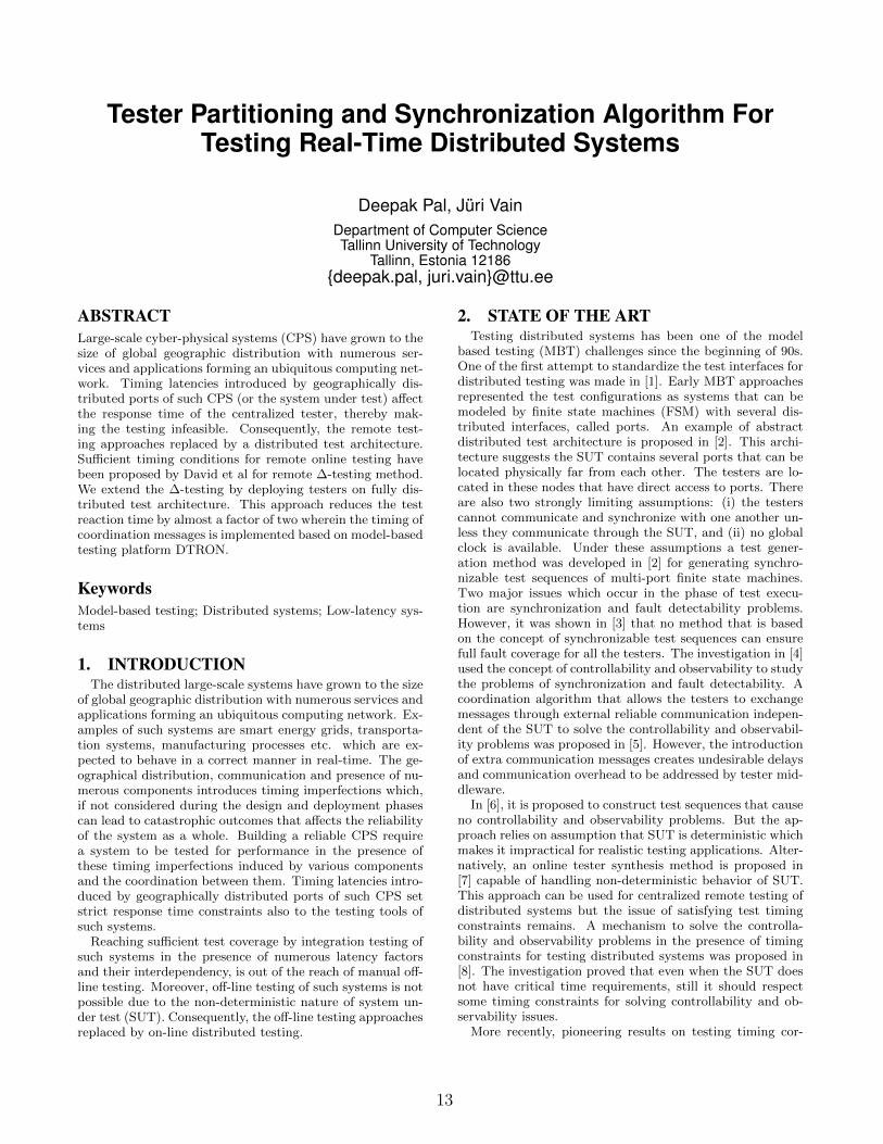
ABSTRACTLarge-scale cyber-physical systems (CPS) have grown to thesize of global geographic distribution with numerous ser-vices and applications forming an ubiquitous computing net-work. Timing latencies introduced by geographically dis-tributed ports of such CPS (or the system under test) affectthe response time of the centralized tester, thereby mak-ing the testing infeasible. Consequently, the remote test-ing approaches replaced by a distributed test architecture.Sufficient timing conditions for remote online testing havebeen proposed by David et al for remote ∆-testing method.We extend the ∆-testing by deploying testers on fully dis-tributed test architecture. This approach reduces the testreaction time by almost a factor of two wherein the timing ofcoordination messages is implemented based on model-basedtesting platform DTRON.
KeywordsModel-based testing; Distributed systems; Low-latency sys-tems
1. INTRODUCTIONThe distributed large-scale systems have grown to the size
of global geographic distribution with numerous services andapplications forming an ubiquitous computing network. Ex-amples of such systems are smart energy grids, transporta-tion systems, manufacturing processes etc. which are ex-pected to behave in a correct manner in real-time. The ge-ographical distribution, communication and presence of nu-merous components introduces timing imperfections which,if not considered during the design and deployment phasescan lead to catastrophic outcomes that affects the reliabilityof the system as a whole. Building a reliable CPS requirea system to be tested for performance in the presence ofthese timing imperfections induced by various componentsand the coordination between them. Timing latencies intro-duced by geographically distributed ports of such CPS setstrict response time constraints also to the testing tools ofsuch systems.
Reaching sufficient test coverage by integration testing ofsuch systems in the presence of numerous latency factorsand their interdependency, is out of the reach of manual off-line testing. Moreover, off-line testing of such systems is notpossible due to the non-deterministic nature of system un-der test (SUT). Consequently, the off-line testing approachesreplaced by on-line distributed testing.
2. STATE OF THE ARTTesting distributed systems has been one of the model
based testing (MBT) challenges since the beginning of 90s.One of the first attempt to standardize the test interfaces fordistributed testing was made in [1]. Early MBT approachesrepresented the test configurations as systems that can bemodeled by finite state machines (FSM) with several dis-tributed interfaces, called ports. An example of abstractdistributed test architecture is proposed in [2]. This archi-tecture suggests the SUT contains several ports that can belocated physically far from each other. The testers are lo-cated in these nodes that have direct access to ports. Thereare also two strongly limiting assumptions: (i) the testerscannot communicate and synchronize with one another un-less they communicate through the SUT, and (ii) no globalclock is available. Under these assumptions a test gener-ation method was developed in [2] for generating synchro-nizable test sequences of multi-port finite state machines.Two major issues which occur in the phase of test execu-tion are synchronization and fault detectability problems.However, it was shown in [3] that no method that is basedon the concept of synchronizable test sequences can ensurefull fault coverage for all the testers. The investigation in [4]used the concept of controllability and observability to studythe problems of synchronization and fault detectability. Acoordination algorithm that allows the testers to exchangemessages through external reliable communication indepen-dent of the SUT to solve the controllability and observabil-ity problems was proposed in [5]. However, the introductionof extra communication messages creates undesirable delaysand communication overhead to be addressed by tester mid-dleware.
In [6], it is proposed to construct test sequences that causeno controllability and observability problems. But the ap-proach relies on assumption that SUT is deterministic whichmakes it impractical for realistic testing applications. Alter-natively, an online tester synthesis method is proposed in[7] capable of handling non-deterministic behavior of SUT.This approach can be used for centralized remote testing ofdistributed systems but the issue of satisfying test timingconstraints remains. A mechanism to solve the controlla-bility and observability problems in the presence of timingconstraints for testing distributed systems was proposed in[8]. The investigation proved that even when the SUT doesnot have critical time requirements, still it should respectsome timing constraints for solving controllability and ob-servability issues.
More recently, pioneering results on testing timing cor-
13
rectness with remote testers was proposed in [9] where aremote abstract tester was proposed for testing distributedsystems in a centralized manner. It was shown that if theSUT ports are remotely observable and controllable then2∆-condition is sufficient for satisfying timing correctness ofthe test. Here, ∆ denotes an upper bound of message prop-agation delay between tester and SUT ports. Though thisapproach works reasonably well for systems with sufficienttiming margins, but it cannot be extended to systems withthe timing constraint close to 2-∆. This means that the testinputs may not reach the input port in time and as a resultthe testing becomes infeasible in such systems.
To shorten the tester reaction time, our recent work [10]proposed an approach for improving the performance of ∆-testing method (proposed originally for single remote tester)by introducing multiple local testers attached directly to theports of SUT on a fully distributed architecture. It wasshown that this mapping to distributed architecture pre-serves the correctness of testers so that if the monolithicremote tester meets 2∆ requirement then the distributedtesters meet (one) ∆-controllability requirement.
In this paper, the main contribution is an improvement ofapproach proposed in [10], which includes following(i) An algorithm that maps a central remote tester model toa set of communicating local tester models while preservingthe I/O behavior at testing ports;(ii) A new adapter model to synchronize the communica-tion between SUT model and local tester and for sendingcoordination messages among local testers.
3. PROBLEM STATEMENT
3.1 Model-Based TestingModel-Based Testing is an approach to the test construc-
tion and test execution process [12]. It is generally under-stood as black-box conformance testing where the goal isto check if the behavior observable on system interface con-forms to a given requirements specification. The formal re-quirements model of SUT describes how the SUT is requiredto behave and allows generating test oracles. The test pur-pose most often used in MBT is conformance testing. Inconformance testing the SUT is considered as a black-box,i.e., only the inputs and outputs of the system are externallycontrollable and observable respectively. During testing, atester executes selected test cases on the SUT and emits atest verdict (pass, fail, inconclusive). The verdict shows cor-rectness in the sense of input-output conformance (IOCO)[11]. Due to native non-determinism of distributed systemsthe natural choice is online testing where the test model isexecuted in lock step with the SUT. The communication be-tween the model and the SUT involves controllable inputsof the SUT and observable outputs of the SUT which makeseasy to detect IOCO violations. For detailed overview ofMBT and related tools we refer to [12].
In our approach Uppaal Timed Automata (UTA) [13] areused as a formalism for modeling SUT behavior. This choiceis motivated by the need to test the SUT with timing con-straints so that the impact of propagation delays betweenthe SUT and the tester can be taken explicitly into accountwhen the test cases are generated and executed. For theformal syntax and semantics of UTA we refer the reader to
[13] and [14].
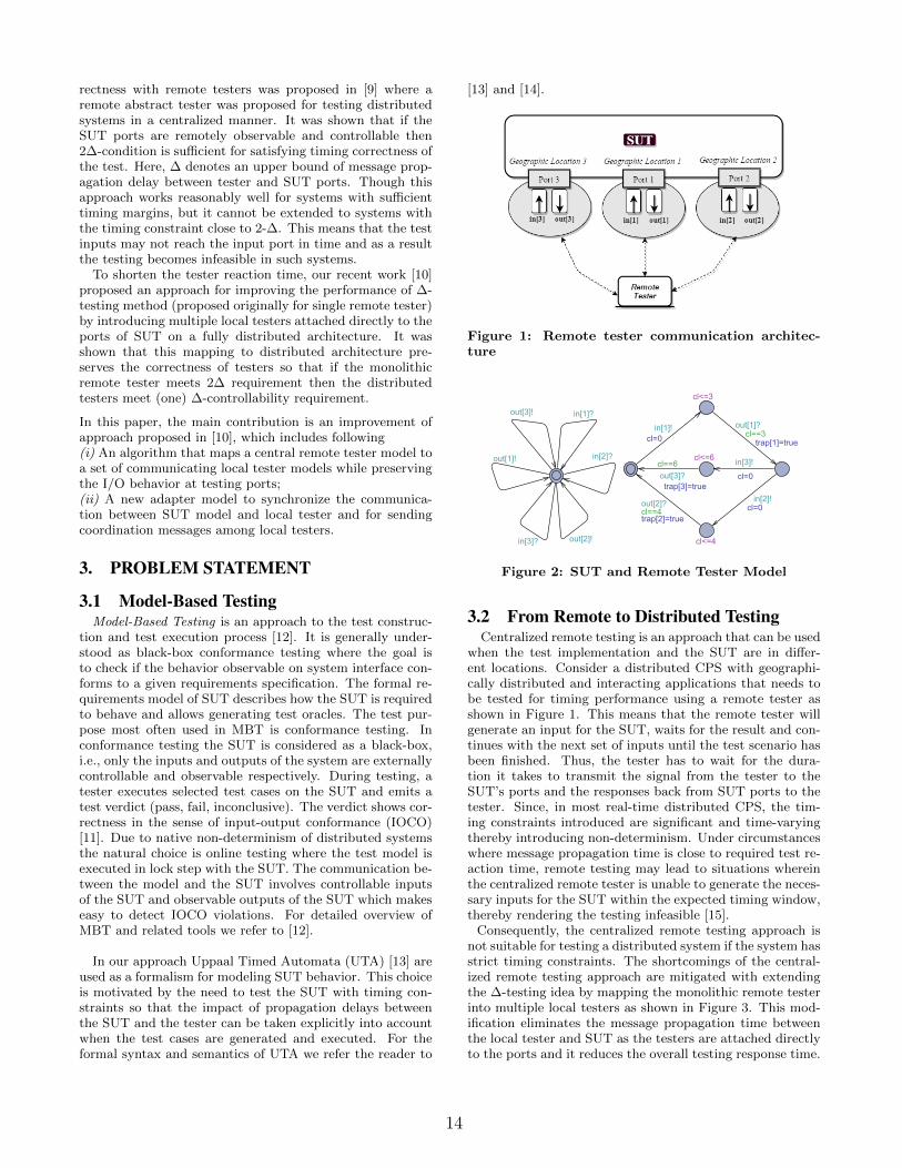
Figure 1: Remote tester communication architec-ture
Figure 2: SUT and Remote Tester Model
3.2 From Remote to Distributed TestingCentralized remote testing is an approach that can be used
when the test implementation and the SUT are in differ-ent locations. Consider a distributed CPS with geographi-cally distributed and interacting applications that needs tobe tested for timing performance using a remote tester asshown in Figure 1. This means that the remote tester willgenerate an input for the SUT, waits for the result and con-tinues with the next set of inputs until the test scenario hasbeen finished. Thus, the tester has to wait for the dura-tion it takes to transmit the signal from the tester to theSUT’s ports and the responses back from SUT ports to thetester. Since, in most real-time distributed CPS, the tim-ing constraints introduced are significant and time-varyingthereby introducing non-determinism. Under circumstanceswhere message propagation time is close to required test re-action time, remote testing may lead to situations whereinthe centralized remote tester is unable to generate the neces-sary inputs for the SUT within the expected timing window,thereby rendering the testing infeasible [15].
Consequently, the centralized remote testing approach isnot suitable for testing a distributed system if the system hasstrict timing constraints. The shortcomings of the central-ized remote testing approach are mitigated with extendingthe ∆-testing idea by mapping the monolithic remote testerinto multiple local testers as shown in Figure 3. This mod-ification eliminates the message propagation time betweenthe local tester and SUT as the testers are attached directlyto the ports and it reduces the overall testing response time.
14

Figure 3: Distributed Local testers communicationarchitecture
4. PARTITIONING ALGORITHMWe apply Algorithm 1 to transform the centralized testing
architecture depicted in Figure 1 into a set of communicatingdistributed local testers, the architecture of which is shownin Figure 3. Let us consider the remote testing architecturein Figure 1 and the corresponding model depicted in Figure2. The SUT has 3 geographically distributed ports (p1, p2,p3) that interact within the system, inputs in[1], in[2] andin[3] at ports p1, p2 and p3 respectively and outputs out[1]at port p1, out[2] at port p2, out[3] at port p3. Now, thelocal testers are generated in two steps:(i) a centralized remote tester is generated, e.g. by applyingthe reactive planning online-tester synthesis method of [7];(ii) a set of synchronizing local testers are derived by map-ping the monolithic tester into a set of location specific testerinstances.
Each tester instance needs to know only the occurrence ofthose I/O events at other ports that influence its behavior.Possible reactions of the local tester to these events are al-ready specified in the initial remote tester model and do notneed further feedback to the event sender. After mappingthe monolithic tester into distributed local testers, the mes-sage propagation time between the local tester and the SUTport is eliminated because the tester is attached directly tothe port. This means the overall testing response time isalso reduced, since previously the messages were transmit-ted twice: from remote tester to the port and back fromport to the tester. The resulting architecture mitigates thetiming issue by replacing the bidirectional communicationwith a unidirectional broadcast of the SUT output signalsbetween the distributed local testers.
Algorithm Description: Assume SUT has n geographi-cally distributed ports, Algorithm 1 generates n communi-cating local testers from monolithic remote tester. Let MRT
denote a monolithic remote tester model generated by ap-plying the reactive planning online-tester synthesis method[7]. Loc(SUT ) denotes a set of geographically different portlocations of SUT . The number of locations Loc(SUT ) ={ln|n ∈ N}. Let Pln denotes a set of ports accessible in thelocation ln. For each port locations ln, ln ∈ Loc(SUT ) wecopy the monolithic remote tester MRT to M ln to be trans-formed to a location specific local tester instance (Line 4-6).Line 7 adds an adapter model to each local tester instance.The purpose of adding an additional automata i.e. adaptersto each location is that it synchronize the local communica-
Algorithm 1 Generating automatically distributed testers.
input : n-port monolithic remote tester modeloutput : n-communicating (LT1, .., LTn) local testers.
1: for all ln, ln ∈ Loc(SUT ) do2: //location specific local tester instance3: copy MRT to M ln
4: add Adapter model to each M ln
5: end for6: for all M ln , n ∈ N do7: for all edges ∈ M ln do8: if (edge.chan[l ] ∧ chan[l ] ∈ Pln) then9: rename & add same chan[l ] to Adapter
10: end if11: if (edge.chan[l ]∧ chan[l ] /∈ Pln) then12: if(chan[l ]! : channel Emission) then13: replace chan[l ]! with co-action Reception
14: rename & add same chan[l ] to Adapter15: end if16: if(chan[l ]? : channel Reception) then17: rename & add same chan[l ] to Adapter18: end if19: end if20: end for21: end for
tion between SUT local ports and a local tester with othertesters in different locations. Its model is derived from re-mote tester model by adding original channels of SUT andby renaming channels of local testers. The loop in Line 9 and10 says that for each local testers model M ln we go throughall the edges in M ln . If the edge has a synchronizing channeland the channel belongs to same port location Pln then werename the chan[l ] shown in Figure 4 and add the samechan[l ] to adapter model (Line 11-13). Second case in Line14-20, if the edge has a synchronizing channel and the chan-nel does not belong to same port location Pln then we do thefollowing (i) if the channel’s action is Emission i.e in[l ]!, wereplace it with the co-action Reception channel, rename itand add it to the adapter model, (ii) if the channel’s actionis Reception i.e out[l ]?, we rename it and add it to adaptermodel.
Figure 4 represents the generated local tester models withtheir corresponding parameterised adapter model where pa-rameter L denotes the geographical location. In this com-position of models it is shown that local testers work to-gether with local adapters. The adapters synchronize thelocal communication between SUT local ports and a localtester with other testers in different locations i.e. in[1] andout[1] are channels between SUT and adapter; in_[1] andout_[1] are channels between the local adapter and localtester; and in__[1] and out__[1] are the channels betweenthe local adapter and other local testers.
5. CORRECTNESS OF TESTER DISTRIBU-TION ALGORITHM
The generated local testers are correct by constructionwhich means that the partitioning preserves their correct-ness because the synchronization of tester local instances ispreserved due to auxiliary synchronization channels intro-duced by the algorithm. Synchronization is preserved alsoamong local testers and with SUT. The communication be-
15
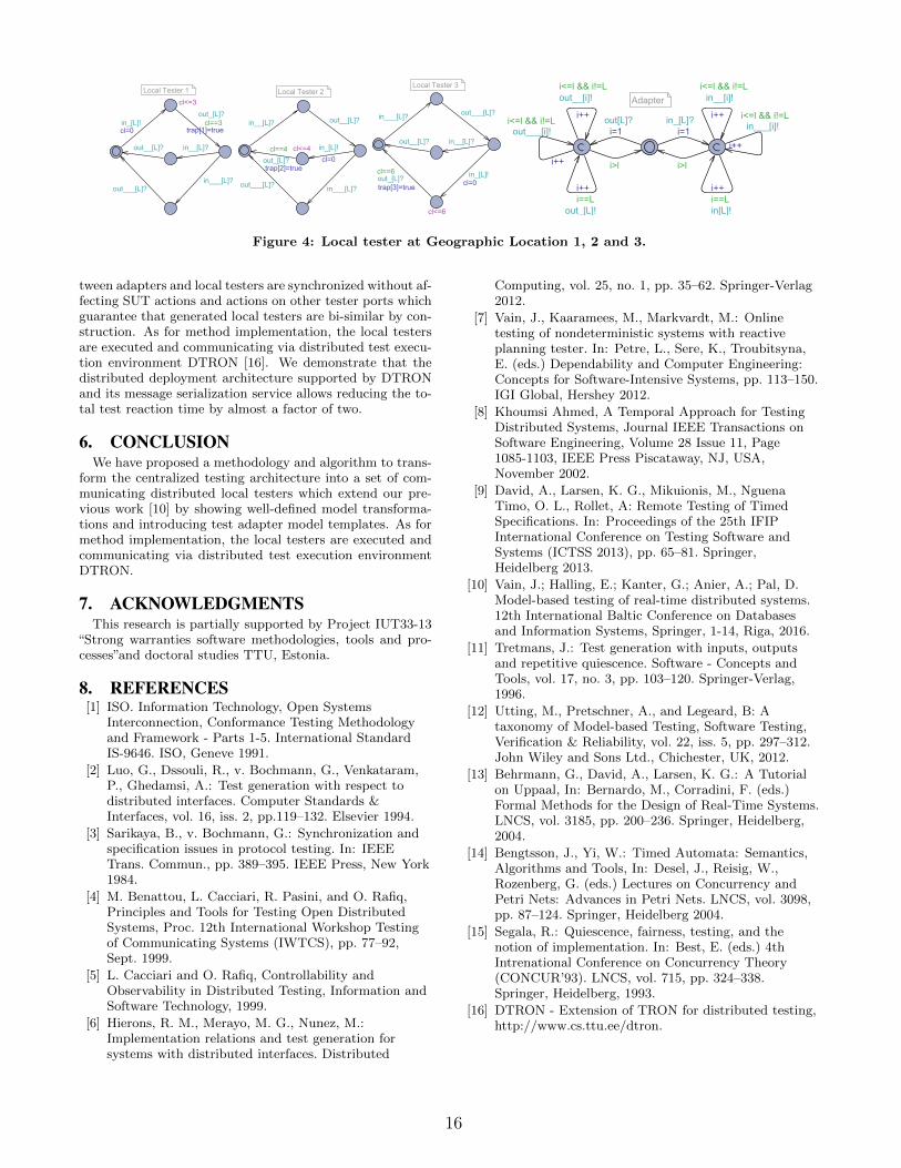
Figure 4: Local tester at Geographic Location 1, 2 and 3.
tween adapters and local testers are synchronized without af-fecting SUT actions and actions on other tester ports whichguarantee that generated local testers are bi-similar by con-struction. As for method implementation, the local testersare executed and communicating via distributed test execu-tion environment DTRON [16]. We demonstrate that thedistributed deployment architecture supported by DTRONand its message serialization service allows reducing the to-tal test reaction time by almost a factor of two.
6. CONCLUSIONWe have proposed a methodology and algorithm to trans-
form the centralized testing architecture into a set of com-municating distributed local testers which extend our pre-vious work [10] by showing well-defined model transforma-tions and introducing test adapter model templates. As formethod implementation, the local testers are executed andcommunicating via distributed test execution environmentDTRON.
7. ACKNOWLEDGMENTSThis research is partially supported by Project IUT33-13
“Strong warranties software methodologies, tools and pro-cesses”and doctoral studies TTU, Estonia.
8. REFERENCES[1] ISO. Information Technology, Open Systems
Interconnection, Conformance Testing Methodologyand Framework - Parts 1-5. International StandardIS-9646. ISO, Geneve 1991.
[2] Luo, G., Dssouli, R., v. Bochmann, G., Venkataram,P., Ghedamsi, A.: Test generation with respect todistributed interfaces. Computer Standards &Interfaces, vol. 16, iss. 2, pp.119–132. Elsevier 1994.
[3] Sarikaya, B., v. Bochmann, G.: Synchronization andspecification issues in protocol testing. In: IEEETrans. Commun., pp. 389–395. IEEE Press, New York1984.
[4] M. Benattou, L. Cacciari, R. Pasini, and O. Rafiq,Principles and Tools for Testing Open DistributedSystems, Proc. 12th International Workshop Testingof Communicating Systems (IWTCS), pp. 77–92,Sept. 1999.
[5] L. Cacciari and O. Rafiq, Controllability andObservability in Distributed Testing, Information andSoftware Technology, 1999.
[6] Hierons, R. M., Merayo, M. G., Nunez, M.:Implementation relations and test generation forsystems with distributed interfaces. Distributed
Computing, vol. 25, no. 1, pp. 35–62. Springer-Verlag2012.
[7] Vain, J., Kaaramees, M., Markvardt, M.: Onlinetesting of nondeterministic systems with reactiveplanning tester. In: Petre, L., Sere, K., Troubitsyna,E. (eds.) Dependability and Computer Engineering:Concepts for Software-Intensive Systems, pp. 113–150.IGI Global, Hershey 2012.
[8] Khoumsi Ahmed, A Temporal Approach for TestingDistributed Systems, Journal IEEE Transactions onSoftware Engineering, Volume 28 Issue 11, Page1085-1103, IEEE Press Piscataway, NJ, USA,November 2002.
[9] David, A., Larsen, K. G., Mikuionis, M., NguenaTimo, O. L., Rollet, A: Remote Testing of TimedSpecifications. In: Proceedings of the 25th IFIPInternational Conference on Testing Software andSystems (ICTSS 2013), pp. 65–81. Springer,Heidelberg 2013.
[10] Vain, J.; Halling, E.; Kanter, G.; Anier, A.; Pal, D.Model-based testing of real-time distributed systems.12th International Baltic Conference on Databasesand Information Systems, Springer, 1-14, Riga, 2016.
[11] Tretmans, J.: Test generation with inputs, outputsand repetitive quiescence. Software - Concepts andTools, vol. 17, no. 3, pp. 103–120. Springer-Verlag,1996.
[12] Utting, M., Pretschner, A., and Legeard, B: Ataxonomy of Model-based Testing, Software Testing,Verification & Reliability, vol. 22, iss. 5, pp. 297–312.John Wiley and Sons Ltd., Chichester, UK, 2012.
[13] Behrmann, G., David, A., Larsen, K. G.: A Tutorialon Uppaal, In: Bernardo, M., Corradini, F. (eds.)Formal Methods for the Design of Real-Time Systems.LNCS, vol. 3185, pp. 200–236. Springer, Heidelberg,2004.
[14] Bengtsson, J., Yi, W.: Timed Automata: Semantics,Algorithms and Tools, In: Desel, J., Reisig, W.,Rozenberg, G. (eds.) Lectures on Concurrency andPetri Nets: Advances in Petri Nets. LNCS, vol. 3098,pp. 87–124. Springer, Heidelberg 2004.
[15] Segala, R.: Quiescence, fairness, testing, and thenotion of implementation. In: Best, E. (eds.) 4thIntrenational Conference on Concurrency Theory(CONCUR’93). LNCS, vol. 715, pp. 324–338.Springer, Heidelberg, 1993.
[16] DTRON - Extension of TRON for distributed testing,http://www.cs.ttu.ee/dtron.
16

Framework to Generate and Validate EmbeddedDecision Trees with Missing Data
Arwa Khannoussi*, Catherine Dezan*, Patrick Meyer+* Université de Bretagne Occidentale
+ Institut Mines-Télécom, Télécom BretagneUMR CNRS 6285 Lab-STICC
[email protected]@univ-brest.fr
ABSTRACTAutonomous vehicles or devices like drones and missilesmust make decisions without human assistance. Em-bedded inference engines, based for example on deci-sion trees, are used to reach this goal which requiresthe respect of hardware and real-time constraints.
This paper proposes a generic framework which cangenerate automatically the adequate hardware solutiontaking into account the real-time and the hardware con-straints. Moreover, the proposed solution supports thecase of faulty sensors which generate missing data.
Experimental results obtained on FPGA and CPUsuggest that it is better to consider missing data fromlearning phase instead of considering it just in the clas-sification phase. Besides, the use of the pipeline tech-nique provides a better latency, which is adequate forreal-time applications.
KeywordsDecision Trees; Missing Data; Hardware Implementa-tion; Real-time; Deadline
1. INTRODUCTIONAutonomous vehicles or devices such as drones or mis-
siles need embedded inference engines to make decisionwithout human assistance. These engines, in their em-bedded version, should respect hardware constraints interms of available resources, performance and energyconsumption. The embedded decision is made with re-spect to data provided by different sensors (GPS, IR,...)with different frequencies. This leads to the definitionof a set of deadlines necessary to manage in real-timethe flow of values provided by the sensors. In this study,we suppose that the sensors can malfunction and con-sequently produce no data.
In machine learning such inference engines includeartificial neural networks [5], decision trees (DTs) [10],support vector machines [13], and many others. In thiswork, we study decision trees, because they are one of
the most popular models and they can easily be inter-preted and validated by humans.
Decision trees are typically constructed from the datausing several algorithms like CART (Classification andRegression Tree) [6], C4.5 [9].. . . Those algorithms canbe implemented and executed on traditional systems.This implementation can not bring a big improvementin term of latency which is an important characteristicto fulfill the real-time constraints. In order to improvedata processing latency and the throughput when con-sidering different instances, a hardware implementationis considered as a solution. However, hardware imple-mentations of decision trees has not been investigatedthoroughly so far.
To our knowledge, [4, 8, 7] are the only three pa-pers available in the literature which discuss the hard-ware implementation of decision trees. Other papers arebased on these seminal references [11, 12]. A. Bermakand D. Martinez [4] propose a hardware realization ofdecision trees using the 2-dimensional systolic array ar-chitecture. J.R. Struharik [8] describes a hardware im-plementation of decision trees for a specific problemonly, while in [7], several architectures are proposedfor the hardware realization of arbitrary decision trees.However, in all those references, the architectures areimplemented manually and each tree has its own imple-mentation.
In this paper we propose a generic framework that al-lows generating decision trees using the C4.5 algorithmbecause it handles training data with missing valuesand generating the adequate hardware solution auto-matically using Vivado HLS tools [1]. Data quality is amajor concern in our work. It is well known that theamount of missing data clearly affects the predictionaccuracy of decision trees. Our framework can there-fore generate, from a configuration, the missing dataand treat them using different methods. As we willshow in this article, this framework actually is a tool tovalidate the hardware solution by comparing its resultswith those of the software solution.
17

The rest of the article is structured as follows. InSection 2, we present the different architectures of thedecision trees hardware implementations that are al-ready proposed in the literature. Section 3 is devotedto the presentation of our framework, and in Section 4we present some experiments and the results with theframework, before concluding in Section 5.
2. RELATED WORKIn general, the input of a machine learning model is
a data set composed of a set of instances evaluated ona set of attributes. For autonomous vehicles or devices,an attribute corresponds to one of the sensors and aninstance includes the values of the different sensors ata given instant. In decision trees, every node of a treerepresents a test that includes one or more attributes,every branch descending from a node represents one ofthe possible outcomes of the test, and every leaf matcheswith one of the classes. To evaluate the performance ofdecision trees we use the classification accuracy, i.e.,the rate of correct predictions made by the model overa data set.
In [8], the realization of the decision tree requires toimplement every node as a separate module. The prob-lem with this architecture is that new instances cannotbe classified before the end of the classification of theprevious ones. A more advanced hardware realizationis proposed in [4]. In order to provide a faster through-put, only two levels are used, irrelevant of the depth ofthe original decision tree.
Several architectures suitable for the hardware real-ization of decision trees are proposed in [7] and arebased on the concept of universal node. Actually, toclassify an instance, one node needs to be evaluated perlevel so only a subset of nodes will be visited, whichcorresponds to the path from the root to the leaf node.The number of modules required for the realization ofa decision tree is equal to the depth of the tree. Oneuniversal node module per level is enough for the real-ization. This Single Module per Level (SMpL) archi-tecture [7] is represented in Figure 1. The classificationof an instance using the SMpL architecture can be ex-ecuted sequentially or with the use of a pipeline. It isalso possible to use a single universal node to evalu-ate every tree node. This architecture, called UniversalNode (UN) [7] (Figure 2), is used when the speed ofclassification is not critical.
The implementation of those architectures is donemanually and each decision tree is therefore implementedseparately. In this contribution, we propose a frame-work which handles this problem. It is an automatictool that can generate an arbitrary decision tree’s struc-ture code on hardware, based on the SMpL architecture.It also allows generating and treat missing data usingseveral methods, and to handle the whole process ofdecision trees learning, from the generation of the deci-sion tree, to the result of the classification in terms of
Figure 1: The Single
Module per Level (SMpL)
architecture for a decision
tree of depth 3 [7].
Figure 2: The struc-
ture of the Universal Node
(UN) architecture [7]
accuracy.
3. PROPOSED FRAMEWORKFigure 3 details the structure of our framework and
the different phases of the implementation.
Figure 3: The structure of the framework.
Besides generating the decision tree structure code,another essential purpose of the framework that we pro-pose is to study the behavior of decision trees when con-fronted with missing data. Therefore, the first part ofour framework is to generate automatically the missingdata by taking as input the data set and the configu-ration of the missing data. Actually, we consider threesuch missing data configurations:
• Uni-variate: missing data appear only in one at-tribute or sensor;
• Monotonic: one or more attributes or sensors areaffected;
• Non-monotonic: missing data appears randomlyin the data set.
18

Note that in our case, typically missing data is causedby a faulty sensor. Missing data can be taken into ac-count during both the learning and the classificationphase. The input of the framework is the data set andmissing data configuration to define which type and thepercentage of missing data will be generated and alsothe number of attributes that will be affected.
The learning phase involves the generation of the de-cision tree from the learning data set. In this phase,an implementation of C4.5 algorithm on R [2] has beenused. C4.5 works with the concept of information en-tropy. The training data is a set of classified sampleshaving p-dimensional vectors defining the attributes ofthe sample. It generates a decision tree where at eachnode C4.5 chooses the attribute that most effectivelysplits its set of samples into subsets enriched in oneclass or other. The splitting criterion is the normal-ized information gain. The attribute with the highestnormalized information gain is chosen to make the de-cision. The output of this phase is the description fileof the decision tree that will be used in the next phase.
The classification phase, can be executed on two dif-ferent device targets, CPU and FPGA. For the first one,we also used the C4.5 algorithm for the classificationand the treatment of missing data. In fact C4.5 usesa probabilistic approach to handle missing data. Thispart of the framework allows testing the decision treewith a number of data sets fixed by the user, and theoutputs are the mean and the standard deviation of thedifferent accuracy rates.
From the decision tree, that has already been gen-erated by the learning phase, our framework generatesautomatically the decision tree structure code, based onthe SMpL architecture [7]. The framework is generictool that can handle any decision tree regardless of thenumber of nodes or the type of attributes, given thattle framework is a generic tool that can handle any de-cision tree. For the missing data, the mean imputationmethod is used. It consists in replacing the missingvalue for a given attribute by the mean of all knownvalues of that attribute. Vivado HLS tools are used toperform the High-Level Synthesis [1].
This framework can manipulate different type of at-tributes, which facilitates the study of the resourcesused in the hardware implementation of the decisiontrees. It produces, the resources used and the latencyas output. In order to validate our hardware imple-mentation, this framework allows comparing it with thesoftware version.
4. EXPERIMENTSIn this section, we first study the behavior of decision
trees when confronted with missing data in both thelearning and the classification phase. Then, the effect ofthe attribute type and the use of pipeline technique onthe required resources are experimented in the hardwareversion of the classification phase.
The following data sets are used to illustrate the useof the framework: “Iris” (4 numerical attributes and 150instances) and “Balance Scale” (4 nominal attributesand 625 instances); see [3] for further details.
As part of the study of the effects of missing data onthe accuracy, we launched a series of experiments onthe software solution. Testing takes place as follows:from the initial data set, the framework generates 1000different data sets with different types and percentage ofmissing data. These are then used in both the learningand classification phases. The results are presented inFigures 4 and 5. Both curves show that classification
Figure 4: Average class.accuracy on “Iris” w.r.t.missing data (%).
Figure 5: Average class.accuracy on “Balance”w.r.t. missing data (%).
accuracy is higher if missing data is already taken intoaccount in the learning phase.
For the classification phase, we suppose that the de-cision tree is already generated. The target device is anFPGA Zynq of the Xilinx Zedboard. For each data set,the following output is produced : the accuracy withmissing data, resource occupation in terms of percent-age of LUT (Lookup Table) and (FF) Flip Flop and thelatency for the performance aspect.
The type of attributes is one of features that can af-fect the performances of decision trees. We thereforeused three different types of attributes for the hardwareimplementation : Float a number coded on 32 bits, ap-ufixed<8,6> a number on 8 bits with 6 integer bits and2 decimal places, and, ap-ufixed<4,2> a number codedon 4 bits with 2 integer bits and 2 decimal places.
Data setAccuracy
Iris Balance
Float <8,6> <4,2> Float <8,6> <4,2>
10 97.15 96.91 88.66 88,94 88,94 41.88
30 94.90 94.57 84.83 86.12 86.12 42.76
50 93.66 93.41 82.16 82.86 82.86 44.24
80 90.49 90.35 78.00 79.56 79.56 45.36
95 88.58 88.40 75.49 78.28 78.28 46.44
Table 1: Classification accuracies with respect to miss-ing data percentages and various types of attributes.
Table 1 shows that classification accuracy decreaseswith increasing amounts of missing data and number ofaffected attributes. Both the type Float and the type
19
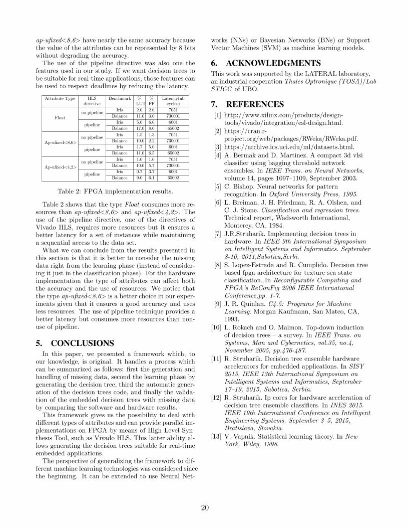
ap-ufixed<8,6> have nearly the same accuracy becausethe value of the attributes can be represented by 8 bitswithout degrading the accuracy.
The use of the pipeline directive was also one thefeatures used in our study. If we want decision trees tobe suitable for real-time applications, those features canbe used to respect deadlines by reducing the latency.
Attribute Type HLSdirective
Benchmark %LUT
%FF
Latency(nbcycles)
Floatno pipeline
Iris 2.0 2.0 7051
Balance 11.0 3.0 730001
pipelineIris 5.0 6.0 6001
Balance 17.0 8.0 65002
Ap-ufixed<8,6>no pipeline
Iris 1.5 1.3 7051
Balance 10.0 2.2 730001
pipelineIris 1.7 5.0 6001
Balance 11.0 6.5 65002
Ap-ufixed<4,2>no pipeline
Iris 1.0 1.0 7051
Balance 10.0 5.7 730001
pipelineIris 0.7 3.7 6001
Balance 9.0 6.1 65002
Table 2: FPGA implementation results.
Table 2 shows that the type Float consumes more re-sources than ap-ufixed<8,6> and ap-ufixed<4,2>. Theuse of the pipeline directive, one of the directives ofVivado HLS, requires more resources but it ensures abetter latency for a set of instances while maintaininga sequential access to the data set.
What we can conclude from the results presented inthis section is that it is better to consider the missingdata right from the learning phase (instead of consider-ing it just in the classification phase). For the hardwareimplementation the type of attributes can affect boththe accuracy and the use of resources. We notice thatthe type ap-ufixed<8,6> is a better choice in our exper-iments given that it ensures a good accuracy and usesless resources. The use of pipeline technique provides abetter latency but consumes more resources than non-use of pipeline.
5. CONCLUSIONSIn this paper, we presented a framework which, to
our knowledge, is original. It handles a process whichcan be summarized as follows: first the generation andhandling of missing data, second the learning phase bygenerating the decision tree, third the automatic gener-ation of the decision trees code, and finally the valida-tion of the embedded decision trees with missing databy comparing the software and hardware results.
This framework gives us the possibility to deal withdifferent types of attributes and can provide parallel im-plementations on FPGA by means of High Level Syn-thesis Tool, such as Vivado HLS. This latter ability al-lows generating the decision trees suitable for real-timeembedded applications.
The perspective of generalizing the framework to dif-ferent machine learning technologies was considered sincethe beginning. It can be extended to use Neural Net-
works (NNs) or Bayesian Networks (BNs) or SupportVector Machines (SVM) as machine learning models.
6. ACKNOWLEDGMENTSThis work was supported by the LATERAL laboratory,an industrial cooperation Thales Optronique (TOSA)/Lab-STICC of UBO.
7. REFERENCES[1] http://www.xilinx.com/products/design-
tools/vivado/integration/esl-design.html.[2] https://cran.r-
project.org/web/packages/RWeka/RWeka.pdf.
[3] https://archive.ics.uci.edu/ml/datasets.html.[4] A. Bermak and D. Martinez. A compact 3d vlsi
classifier using bagging threshold networkensembles. In IEEE Trans. on Neural Networks,volume 14, pages 1097–1109, September 2003.
[5] C. Bishop. Neural networks for patternrecognition. In Oxford University Press, 1995.
[6] L. Breiman, J. H. Friedman, R. A. Olshen, andC. J. Stone. Classification and regression trees.Technical report, Wadsworth International,Monterey, CA, 1984.
[7] J.R.Struharik. Implementing decision trees inhardware. In IEEE 9th International Symposiumon Intelligent Systems and Informatics. September8-10, 2011,Subotica,Serbi.
[8] S. Lopez-Estrada and R. Cumplido. Decision treebased fpga architecture for texture sea stateclassification. In Reconfigurable Computing andFPGA’s ReConFig 2006 IEEE InternationalConference,pp. 1-7.
[9] J. R. Quinlan. C4.5: Programs for MachineLearning. Morgan Kaufmann, San Mateo, CA,1993.
[10] L. Rokach and O. Maimon. Top-down inductionof decision trees – a survey. In IEEE Trans. onSystems, Man and Cybernetics, vol.35, no.4,November 2005, pp.476-487.
[11] R. Struharik. Decision tree ensemble hardwareaccelerators for embedded applications. In SISY2015, IEEE 13th International Symposium onIntelligent Systems and Informatics, September17–19, 2015, Subotica, Serbia.
[12] R. Struharik. Ip cores for hardware acceleration ofdecision tree ensemble classifiers. In INES 2015.IEEE 19th International Conference on IntelligentEngineering Systems. September 3–5, 2015,Bratislava, Slovakia.
[13] V. Vapnik. Statistical learning theory. In NewYork, Wiley, 1998.
20

Quantifying the Flexibility of Real-Time SystemsRafik Henia1, Alain Girault2, Christophe Prévot1,2, Sophie Quinton2, Laurent Rioux1
1 Thales Research & Technology2 Inria Grenoble Rhône-Alpes
1. INTRODUCTIONThe life cycle of many safety or mission critical real-time
systems, such as avionic systems, satellites or software de-fined radios, is superior to 10 years whereas the supportingICT technologies have a much faster evolution rate. Thismismatch between system life cycle on one side and softwarelife cycle on the other side is a challenge for performanceengineers. It is therefore essential for commercial offers toallow technology evolutions and upgrades of the architectureand functions after the initial system deployment. Besides,this must be done while preserving the satisfaction of timingperformance requirements over the entire system lifetime.
Our objective is to develop novel techniques to quantifythe ability of a real-time system to cope with future soft-ware evolutions, while remaining schedulable. We proposeto define the flexibility of a system as its ability to schedulea new software function and show how this concept can beused to anticipate at design time schedulability bottlenecksthat may prove problematic, after deployment, for systemevolution. In this paper we focus on an evolution scenariowhere a single task is added to an existing system running ona single-core processor. Our task model here is restricted toindependent periodic tasks with implicit deadlines and thescheduling policy is static priority preemptive. Of course ourgoal is to generalize our approach to more complex systems.
The research area that is most closely related to our prob-lem is sensitivity analysis [9, 2, 5, 7]. Sensitivity analysis isused (1) to provide guarantees on the schedulability of a sys-tem in case of uncertainty on the system parameters, or (2)given a non schedulable system, to find a set of changes thatlead to a schedulable system.
Most related work on sensitivity analysis addresses changesof one type of parameter, e.g., changes of task worst-caseexecution times (WCETs) or changes of periods — but notboth. In [2] for example, the authors analyze the sensitivityof a system to changes in the arrival frequency of all tasks, orin the WCET of all tasks. In [7], the authors are interestedin sensitivity analysis of systems with shared resources, forwhich they study the impact of an increase of the WCETson system schedulability.
Dealing with different parameters (i.e. periods and prior-ities) is the approach used in [8]. Here the authors definethe sensitivity using evolutionary algorithms and a stochas-tic approach. It will be interesting to compare our resultswith this method.
In contrast with the above mentioned approaches, we donot allow parameters of the deployed system to be modi-fied in according with industrial practice. But we need to
handle at the same time changes in the period, priority andWCET of the task to be added. As a result, the set of pos-sible system configurations that need to be checked is muchsmaller than in classical sensitivity analysis and we hope tobe able to handle much more complex systems that whatstate-of-the-art sensitivity analysis can handle.
Other papers like [10, 1, 3] deal with flexibility related totask allocation, priority assignment or scenario based opti-mization. In [3], the authors use concepts similar to ours todefine an optimal or a robust priority assignment. In [10],the authors deal with task allocation and priority assignmentto maximize the extensibility of each task chain, where ex-tensibility is the maximum execution time it is possible toincrease the WCET before missing the deadline. In [1] theflexibility of a system is defined according to scenarios. Todefine the flexibility it is necessary to define possible scenar-ios of change.
Related work that deals with flexibility is used to defineat design time what is the best task allocation or priority as-signment. But most of the time in an industrial context, thedesigner cannot take into account only timing constraintsand some functionalities have fixed parameters. Moreoverwe are interested in system evolution when most parametersof the system are already defined. It is at this point unclearif our problem (adding a task) can be precisely encoded intoexisting methods dealing with increased execution times.
As a summary, by restricting ourselves to a simple changescenario with industrial relevance, we hope to come up withan approach that can provide guidance for the evolutionof complex systems, which cannot be covered by existingsensitivity analysis techniques. Finally, to the best of ourknowledge, no existing work discusses the notion of limitingtask, i.e. the task which will miss its deadline first. Thefinal aim is to help the designer by giving him information toallow a system to evolve while respecting timing constraints.
2. SYSTEM MODELUnless otherwise specified all the parameters defined in
the following have positive integer values. In particular, weassume a discrete time clock.
We consider a uni-processor real-time system S consistingof a finite set of n independent tasks scheduled accordingto the Static Priority Preemptive (SPP) scheduling policy.Each task τi, i ∈ [1, n], is defined by a tuple (πi, Ti, Ci) whereπi is the priority, Ti the period, and Ci an upper-bound onthe worst case execution time (WCET). Each task τi has animplicit deadline Di = Ti, meaning that a given activationof τi must finish before the next activation of τi.
21
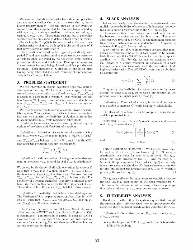
We assume that different tasks have different prioritiesand use as convention that πi < πj means that τi has ahigher priority than τj . For the purpose of our evolutionscenario, we also suppose that for any two tasks τi and τjwith πi < πj , it is always possible to define a new task τnewwith πi < πnew < πj . This is done without loss of generalityas priorities are only used to define a total order on tasks.
For each τi in S, hp(i) is the set of tasks of S that havea higher priority than τi, while lp(i) is the set of tasks of Sthat have a lower priority than τi.
The execution of a task τi is triggered periodically withperiod Ti and each activation of τi generates a new instance.A task instance is defined by its activation time, possiblepreemption delays, and finish time. Preemption delays aredue to the task instance being blocked by higher priority taskinstances. Each instance of τi finishes at the latest afterhaving being scheduled (i.e., not counting the preemptiondelays) for Ci units of time.
3. PROBLEM STATEMENTWe are interested in system evolutions that may happen
after system delivery. We focus here on a simple evolutionscenario where a new task τnew defined by (πnew, Tnew, Cnew)is added to a schedulable system S, thus yielding the sys-tem Snew = S ∪ {τnew}. From now on, τnew will denote thetask (πnew, Tnew, Cnew) and Snew will denote the systemS ∪ {τnew}.
We wish to answer the following question: Given a schedu-lable system S and a task τnew with unknown parameters:how can we quantify the flexibility of S, that is, its abilityto accommodate τnew while remaining schedulable?
To address these issues, we start below by formalizing thenotions of evolution and flexibility of a system.
Definition 1. Evolution: An evolution of a system S is atask τnew where πnew belongs to [min
iπi−1,max
iπi+1]\{πi}i
and (Tnew, Cnew) belongs to N+ × N+, such that the CPUload after the evolution does not exceed 100%:
CnewTnew
+∑i
CiTi≤ 1
Definition 2. Valid evolution: S being a schedulable sys-tem, an evolution τnew is valid for S if Snew is schedulable.
We denote by FS the set of all valid evolutions for system S.Note that if τnew is in FS , then for any 0 < C′
new < Cnew,the task (πnew, Tnew, C
′new) is also in FS . Moreover for any
T ′new > Tnew, the task (πnew, T
′new, Cnew) is also in FS . The
flexibility of a system quantifies its ability to schedule a newtask. We focus in this paper on the flexibility w.r.t. Cnew.The notion of flexibility w.r.t. Tnew is left for future work.
Definition 3. Flexibility: Let S be a schedulable system.The flexibility of S is the partial function flexS from N+×N+
into N+ such that (πnew, Tnew,flexS(πnew, Tnew)) is in FSand flexS(πnew, Tnew) is maximal.
The function flex returns, for all (πnew, Tnew), the valueof the maximum WCET such that S ∪ {(π, T,flexS(π, T ))}is schedulable. This function is partial as such an WCETmay not exist. In the rest of the paper, we first focus onmethods for computing flex and then we will show how wecan use it for system design.
4. SLACK ANALYSISLet us first briefly recall the standard analysis used to es-
tablish the schedulability of systems of independent periodictasks on a single processor under the SPP policy [6].
The response time of an instance of a task τi is the de-lay between its activation and its finish time. The worstcase response time of τi (WCRT) is the maximum responsetime over all instances of τi; it is denoted ri. A system isschedulable if ri ≤ Ti for any task τi.
A critical instant of τi is an activation scenario that max-imises the response time of τi. A task is said to be schedu-lable if and only if its WCRT is smaller than its (implicit)deadline: ri ≤ Ti. For the systems we consider, a crit-ical instant of τi occurs whenever an activation of a taskinstance occurs simultaneously with the activation of allhigher-priority tasks. The WCRT of τi can thus be obtainedby computing:
ri = Ci +∑
τj∈hp(i)
⌈riTj
⌉Cj (1)
To quantify the flexibility of a system, we start by intro-ducing the slack of a task, which takes into account all thepreemptions from higher priority tasks [4].
Definition 4. The slack of a task τi is the maximum valueit is possible to increase Ci while keeping τi schedulable.
The slack Sl i of a task τi can be computed using the al-gorithm presented in [4].
Theorem 1. Let S be a schedulable system and τnew atask. Snew is schedulable if:
∀τi ∈ lp(new),
⌈TiTnew
⌉Cnew ≤ Sl i (2)
andrnew ≤ Tnew (3)
Proof sketch of Theorem 1. We have to prove that,for each τi ∈ S ∪ {τnew}, we have ri ≤ Ti. Since S isschedulable, this holds for each τh ∈ hp(new). For τnewitself, this holds directly by Eq. (3). And for each τ` ∈lp(new), the preemptions of the tasks in hp(`) are alreadytaken into account in the slack Sl`, hence there only remainsto take into account the preemptions of τnew on τ`, which isprecisely the goal of Eq. (2).
This gives a sufficient but non necessary condition becausethe slack Sli is a lower bound on the slack available for τi.The reason the criterion is not necessary is that the preemp-tion delays induced by τnew may be overapproximated.
5. FLEXIBILITY ANALYSISRecall that the flexibility of a system is quantified through
the function flex . We now show how to approximate flexusing the above sufficient schedulability condition for Snew.
Definition 5. For a given period Tnew and priority πnewof τnew, denote
• CS the largest WCET of τnew such that S is schedu-lable after evolving,
22

• Cτnew the largest WCET of τnew such that τnew isschedulable after evolving.
Theorem 2. S being a system and τnew an evolution, letCmaxS be the largest WCET allowed by Eq. (2) i.e. a lowerbound of CS. Let Cmaxτnew
be the largest WCET allowed byEq. (3) i.e. a lower bound of Cτnew . Then
CmaxSnew= min {CmaxS , Cmaxτnew
}
is a lower bound of flexS(πnew, Tnew).
Proof sketch of Theorem 2. Theorem 1 gives a guar-antee on the schedulability of Snew depending on τnew whichis a sufficient non necessary condition. As a consequence,Theorem 2 based on Theorem 1 is also a sufficient and nonnecessary condition, i.e., a lower bound of the largest Cnewthat guarantees the schedulability of Snew for fixed πnew andTnew — which is given by flexS .
We can compute both CmaxS and Cmaxτnewusing Theorem 3.
Theorem 3. Let S be a schedulable system and τnew atask. Then we have CmaxS and Cmaxτnew
:
CmaxS = minτi∈lp(new)
Sl i⌈Ti
Tnew
⌉ (4)
and
Cmaxτnew=
Tnew − ∑τj∈hp(new)
⌈TnewTj
⌉Cj
(5)
Proof. Eq. (2) implies that, for all task τi in lp(new),we have Cnew ≤ Sli/d Ti
Tnewe. Since Cnew must be in N+, it
follows that
Cnew ≤ minτi∈lp(new)
⌊Sli/d
TiTnew
e⌋
hence Eq. (4). We found the largest Cnew by computing thelargest Slnew. Again, since Cnew must be in N+, this leadsto Eq. (5).
Intuitively, if τnew has a high priority, then it will be easyto schedule but it will have a stronger impact on S. Andthis impact will be greater if the period Tnew is small. Incontrast, a task τnew with a low priority will have a smallerimpact on the other tasks and it will be harder to schedulewith a small period.
Note that the function flexS is partial. Both Conditions (4)and (5) on the flexibility of τnew imply that some tuples(πnew, Tnew) lead to non schedulable systems. These tuplesimply that at least one task in Snew will have not enoughtime to be executed. This is the case in a system if we addτnew with a high priority and a small period.
6. LIMITING TASK OF THE SYSTEMWe now focus on the fact that for a priority πnew and
a period Tnew, CmaxS is limited by one, or possibly severaltasks in lp(new). We call the lowest priority task amongthem the limiting task.
Definition 6. The limiting task of S w.r.t. a priority πnewand a period Tnew, denoted τ`, is the lowest priority task τ`such that:
` = arg minτi∈lp(new)
Sl i⌈Ti
Tnew
⌉ (6)
Note that our definition of limiting task is based on thesufficient condition in Theorem 1. As a result, it is a goodindicator of where the bottlenecks for software evolution are,but it is not an exact criterion (yet).
We are particularly interested in the fact that some tasksnever limit CmaxS , whatever the priority and period of τnew.
Theorem 4. Consider the system S. The tasks that willnever limit the system are all the tasks τi such that:
∃τj ∈ S s.t. τj ∈ lp(i) ∧ Tj ≤ Ti
Proof sketch of Theorem 4. Tasks for which there ex-ists another task of lower priority (hence with more preemp-tions) and lesser or equal period (hence with less or the sameavailable time to finish) can never be the limiting task.
A good strategy to increase the flexibility of the system isto decrease the interference of higher priority tasks on thelimiting task τ`, i.e., to increase its slack. One source ofcomplexity here is that the limiting task is not necessarilythe same for different values of Tnew and πnew.
We therefore identify the values of the period Tnew uponwhich τ` may change. The set of these values is:
T =
{t ∈ N+ | ∃τi ∈ S,
⌈Tit
⌉6=⌈Tit− 1
⌉}(7)
This corresponds to the values of Tnew for which the numberof preemptions of τnew on τi, with i ∈ lp(new), changes. Itfollows that τ` remains constant in any interval [T inew, T
jnew[
where T inew and T jnew are two consecutive periods in T . It isthus sufficient to compute the limiting task of S w.r.t. eachpriority πnew and period of Tnew ∈ T using Eq. (6).
7. CASE STUDYLet us now show how the concepts presented in this paper
are applied on an example. Consider a system:
S = {(2, 10, 1), (4, 5, 1), (6, 15, 1), (8, 10, 2), (10, 30, 2)}
Case 1: Priority and period of τnew are knownSuppose that we want to add a task τnew to S, with πnew = 1and Tnew = 5. By applying Theorem 3 and Definition 6 wedetermine that CmaxS = 1 and τ5 is the limiting task of S.This means that τnew should not have an execution timelarger than 1 otherwise τ5 may miss its deadline.
Case 2: CmaxS as a function of TnewLet us now assume that we know nothing about τnew andwe want to quantify the flexibility of S.
Table 1 shows the values of CmaxS obtained for the possi-ble values of πnew and τnew. Whenever any WCET largerthan 0 would make one task in S unschedulable we put ⊥.Note that we group periods of τnew for which the numberof preemptions of tasks in S does not change, based on thecomputation of T . In addition, if πnew ≥ 11 then τnew willhave no impact on the system so we do not represent Cmaxnew .
Similarly, Table 2 shows Cmaxτnewfor possible values of πnew
and Tnew (we leave out periods larger than 15). Finally,based on Table 1 and Table 2 we easily obtain Table 3 whichshows the possible values of CmaxSnew
.The concepts introduced in this paper allow the system
designer to: (1) understand when an evolution will be con-strained by the need to preserve the schedulability of the sys-tem, and when it will be constrained by the need to schedule
23

aaaaaaTnew
πnew 1 3 5 7 9
[2, 3[ ⊥ ⊥ ⊥ ⊥ ⊥[3, 4[ 1 1 1 1 1[4, 5[ 1 1 1 1 1[5, 6[ 1 1 1 1 1[6, 8[ 2 2 2 2 2[8, 10[ 2 2 2 2 2[10, 15[ 3 3 3 3 3[15, 30[ 3 3 4 4 5[30, +∞[ 3 3 4 4 11
Table 1: CmaxS for different values of πnew and Tnew
aaaaaaTnew
πnew 3 5 7 9 11
2 1 ⊥ ⊥ ⊥ ⊥3 2 1 ⊥ ⊥ ⊥4 3 2 1 ⊥ ⊥5 4 3 2 ⊥ ⊥6 5 3 2 ⊥ ⊥7 6 4 3 1 ⊥8 7 5 4 2 ⊥9 8 6 5 3 110 9 7 6 4 211 9 6 5 1 ⊥12 10 7 6 2 ⊥13 11 8 7 3 114 12 9 8 4 215 13 10 9 5 3
Table 2: Cmaxτnewfor different values of πnew and Tnew
the new task; (2) identify, through the concept of limitingtask, which task in the system will “break” first in case of asoftware update.
8. CONCLUSIONIn this paper we have defined the flexibility of a system as
its capability to schedule a new task. We also presented anapproach to quantify the flexibility of a system. More impor-tantly, we show that it is possible under certain conditionsto identify the task that will directly induce the limitationson a possible software update. If performed at design time,such a result can be used to adjust the system design bygiving more slack to the limiting task. We illustrate howthese results apply to a simple system.
We plan to extend our work in several main directions.First, we want to replace our sufficient conditions for bynecessary and sufficient conditions so as to provide morerelevant information to the system designer.
Second, we want to study further the notion of limitingtask and propose a solution to compare the flexibility ofdifferent systems. Our objective is to come up with a set ofguidelines for the designer to help him factor in flexibility atdesign time. Such guidelines must be simple to understandby someone with limited expertise in schedulability analysis,and they must take into account the fact that many designchoices are fixed.
Finally, we intend to study more complex systems. Weare in particular interested in systems with jitter, sporadic
aaaaaaTnew
πnew 1 3 5 7 9 11
2 ⊥ ⊥ ⊥ ⊥ ⊥ ⊥3 1 1 1 ⊥ ⊥ ⊥4 1 1 1 1 ⊥ ⊥5 1 1 1 1 ⊥ ⊥6 2 2 2 2 ⊥ ⊥7 2 2 2 2 1 ⊥8 2 2 2 2 2 ⊥9 2 2 2 2 2 110 3 3 3 3 3 211 3 3 3 3 1 ⊥12 3 3 3 3 2 ⊥13 3 3 3 3 3 114 3 3 3 3 3 215 3 3 4 4 5 3
Table 3: CmaxSnewfor different values of πnew and Tnew
bursts, task chains, multiple processing resources, etc. Whencompared to the general sensitivity analysis problem, theproblem we consider has many fixed parameters. This iswhy we expect to be able to provide useful results even forsuch complex systems.
9. REFERENCES
[1] I. Bate and P. Emberson. Incorporating scenarios andheuristics to improve flexibility in real-time embeddedsystems. In RTAS’06, pages 221–230, San Jose (CA),USA, 2006. IEEE.
[2] E. Bini, M. Di Natale, and G. Buttazzo. Sensitivityanalysis for fixed-priority real-time systems. InECRTS’06, pages 13–22. IEEE, 2006.
[3] R. Davis and A. Burns. Robust priority assignment forfixed priority real-time systems. In RTSS’07, pages3–14. IEEE, 2007.
[4] R. I. Davis, K. Tindell, and A. Burns. Schedulingslack time in fixed priority pre-emptive systems. InRTSS’93, pages 222–231, 1993.
[5] F. Dorin, P. Richard, M. Richard, and J. Goossens.Schedulability and sensitivity analysis of multiplecriticality tasks with fixed-priorities. Real-Time Syst.,46(3):305–331, 2010.
[6] M. Joseph and P. Pandya. Finding response times in areal-time system. The Computer Journal,29(5):390–395, 1986.
[7] S. Punnekkat, R. Davis, and A. Burns. Sensitivityanalysis of real-time task sets. In ASIAN’97, volume1345 of LNCS, pages 72–82. Springer-Verlag, 1997.
[8] R. Racu, A. Hamann, and R. Ernst. Sensitivityanalysis of complex embedded real-time systems.Real-Time Syst., 39(1-3):31–72, 2008.
[9] R. Racu, M. Jersak, and R. Ernst. Applyingsensitivity analysis in real-time distributed systems. InRTAS’05, pages 160–169. IEEE, 2005.
[10] Q. Zhu, Y. Yang, E. Scholte, M. Di Natale, andA. Sangiovanni-Vincentelli. Optimizing extensibility inhard real-time distributed systems. In RTAS’09, pages275–284. IEEE, 2009.
24
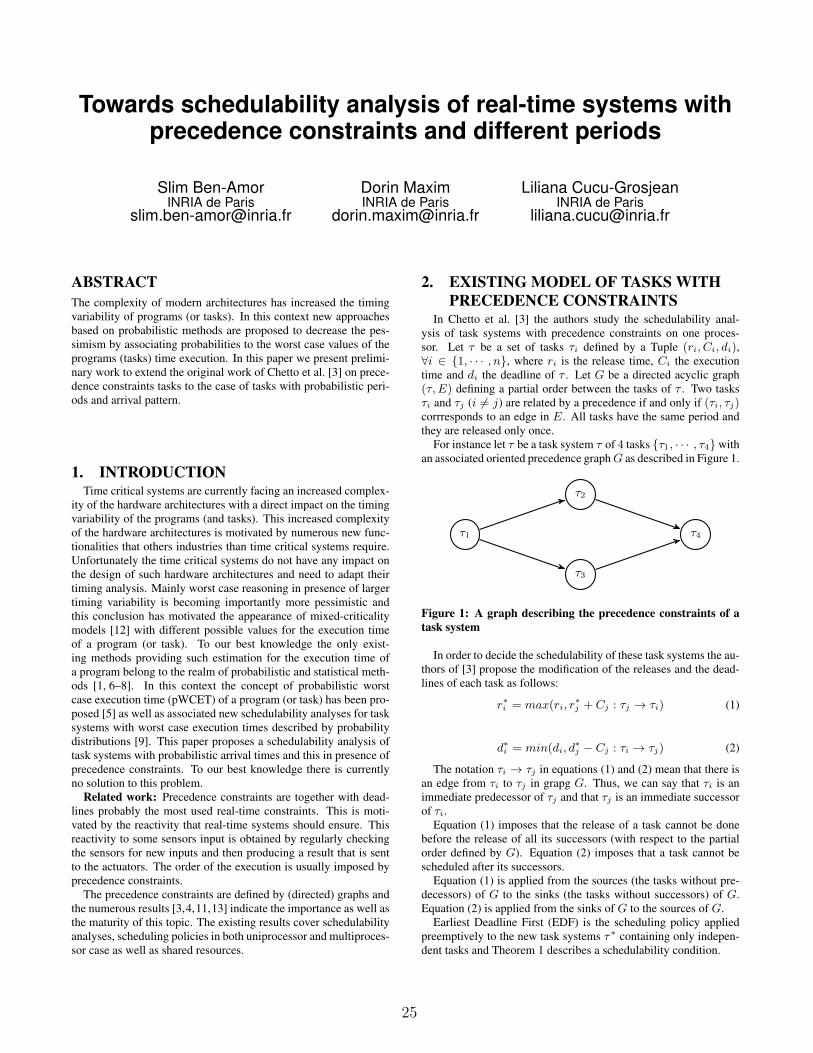
Towards schedulability analysis of real-time systems withprecedence constraints and different periods
Slim Ben-AmorINRIA de Paris
Dorin MaximINRIA de Paris
Liliana Cucu-GrosjeanINRIA de Paris
ABSTRACTThe complexity of modern architectures has increased the timingvariability of programs (or tasks). In this context new approachesbased on probabilistic methods are proposed to decrease the pes-simism by associating probabilities to the worst case values of theprograms (tasks) time execution. In this paper we present prelimi-nary work to extend the original work of Chetto et al. [3] on prece-dence constraints tasks to the case of tasks with probabilistic peri-ods and arrival pattern.
1. INTRODUCTIONTime critical systems are currently facing an increased complex-
ity of the hardware architectures with a direct impact on the timingvariability of the programs (and tasks). This increased complexityof the hardware architectures is motivated by numerous new func-tionalities that others industries than time critical systems require.Unfortunately the time critical systems do not have any impact onthe design of such hardware architectures and need to adapt theirtiming analysis. Mainly worst case reasoning in presence of largertiming variability is becoming importantly more pessimistic andthis conclusion has motivated the appearance of mixed-criticalitymodels [12] with different possible values for the execution timeof a program (or task). To our best knowledge the only exist-ing methods providing such estimation for the execution time ofa program belong to the realm of probabilistic and statistical meth-ods [1, 6–8]. In this context the concept of probabilistic worstcase execution time (pWCET) of a program (or task) has been pro-posed [5] as well as associated new schedulability analyses for tasksystems with worst case execution times described by probabilitydistributions [9]. This paper proposes a schedulability analysis oftask systems with probabilistic arrival times and this in presence ofprecedence constraints. To our best knowledge there is currentlyno solution to this problem.
Related work: Precedence constraints are together with dead-lines probably the most used real-time constraints. This is moti-vated by the reactivity that real-time systems should ensure. Thisreactivity to some sensors input is obtained by regularly checkingthe sensors for new inputs and then producing a result that is sentto the actuators. The order of the execution is usually imposed byprecedence constraints.
The precedence constraints are defined by (directed) graphs andthe numerous results [3,4,11,13] indicate the importance as well asthe maturity of this topic. The existing results cover schedulabilityanalyses, scheduling policies in both uniprocessor and multiproces-sor case as well as shared resources.
2. EXISTING MODEL OF TASKS WITHPRECEDENCE CONSTRAINTS
In Chetto et al. [3] the authors study the schedulability anal-ysis of task systems with precedence constraints on one proces-sor. Let τ be a set of tasks τi defined by a Tuple (ri, Ci, di),∀i ∈ {1, · · · , n}, where ri is the release time, Ci the executiontime and di the deadline of τ . Let G be a directed acyclic graph(τ, E) defining a partial order between the tasks of τ . Two tasksτi and τj (i 6= j) are related by a precedence if and only if (τi, τj)corrresponds to an edge in E. All tasks have the same period andthey are released only once.
For instance let τ be a task system τ of 4 tasks {τ1, · · · , τ4}withan associated oriented precedence graphG as described in Figure 1.
τ1
τ2
τ3
τ4
Figure 1: A graph describing the precedence constraints of atask system
In order to decide the schedulability of these task systems the au-thors of [3] propose the modification of the releases and the dead-lines of each task as follows:
r∗i = max(ri, r∗j + Cj : τj → τi) (1)
d∗i = min(di, d∗j − Cj : τi → τj) (2)
The notation τi → τj in equations (1) and (2) mean that there isan edge from τi to τj in grapg G. Thus, we can say that τi is animmediate predecessor of τj and that τj is an immediate successorof τi.
Equation (1) imposes that the release of a task cannot be donebefore the release of all its successors (with respect to the partialorder defined by G). Equation (2) imposes that a task cannot bescheduled after its successors.
Equation (1) is applied from the sources (the tasks without pre-decessors) of G to the sinks (the tasks without successors) of G.Equation (2) is applied from the sinks of G to the sources of G.
Earliest Deadline First (EDF) is the scheduling policy appliedpreemptively to the new task systems τ∗ containing only indepen-dent tasks and Theorem 1 describes a schedulability condition.
25
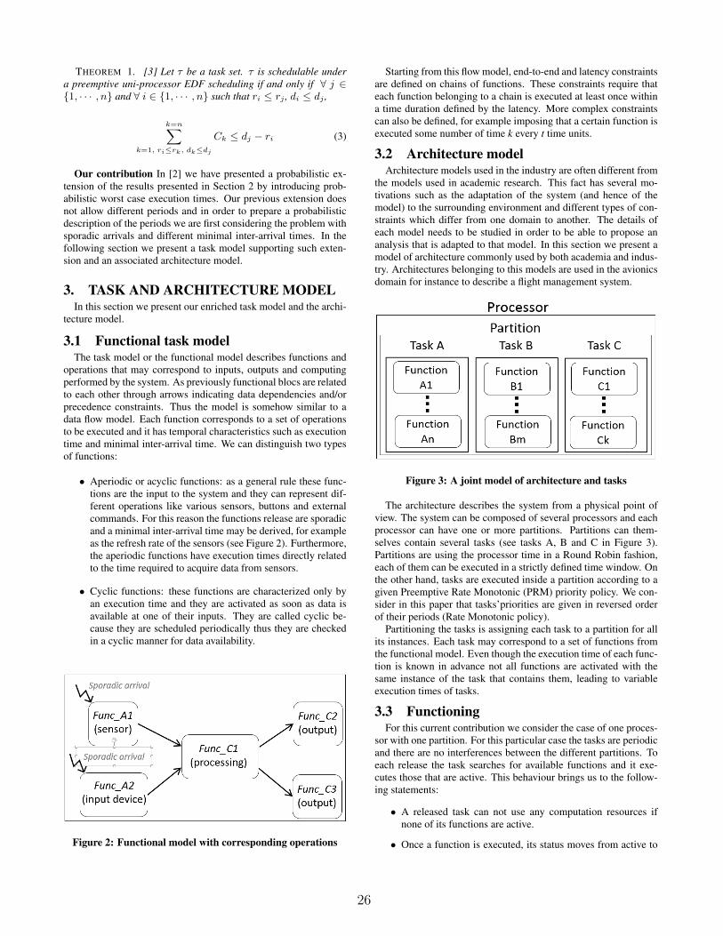
THEOREM 1. [3] Let τ be a task set. τ is schedulable undera preemptive uni-processor EDF scheduling if and only if ∀ j ∈{1, · · · , n} and ∀ i ∈ {1, · · · , n} such that ri ≤ rj , di ≤ dj ,
k=n∑k=1, ri≤rk, dk≤dj
Ck ≤ dj − ri (3)
Our contribution In [2] we have presented a probabilistic ex-tension of the results presented in Section 2 by introducing prob-abilistic worst case execution times. Our previous extension doesnot allow different periods and in order to prepare a probabilisticdescription of the periods we are first considering the problem withsporadic arrivals and different minimal inter-arrival times. In thefollowing section we present a task model supporting such exten-sion and an associated architecture model.
3. TASK AND ARCHITECTURE MODELIn this section we present our enriched task model and the archi-
tecture model.
3.1 Functional task modelThe task model or the functional model describes functions and
operations that may correspond to inputs, outputs and computingperformed by the system. As previously functional blocs are relatedto each other through arrows indicating data dependencies and/orprecedence constraints. Thus the model is somehow similar to adata flow model. Each function corresponds to a set of operationsto be executed and it has temporal characteristics such as executiontime and minimal inter-arrival time. We can distinguish two typesof functions:
• Aperiodic or acyclic functions: as a general rule these func-tions are the input to the system and they can represent dif-ferent operations like various sensors, buttons and externalcommands. For this reason the functions release are sporadicand a minimal inter-arrival time may be derived, for exampleas the refresh rate of the sensors (see Figure 2). Furthermore,the aperiodic functions have execution times directly relatedto the time required to acquire data from sensors.
• Cyclic functions: these functions are characterized only byan execution time and they are activated as soon as data isavailable at one of their inputs. They are called cyclic be-cause they are scheduled periodically thus they are checkedin a cyclic manner for data availability.
Figure 2: Functional model with corresponding operations
Starting from this flow model, end-to-end and latency constraintsare defined on chains of functions. These constraints require thateach function belonging to a chain is executed at least once withina time duration defined by the latency. More complex constraintscan also be defined, for example imposing that a certain function isexecuted some number of time k every t time units.
3.2 Architecture modelArchitecture models used in the industry are often different from
the models used in academic research. This fact has several mo-tivations such as the adaptation of the system (and hence of themodel) to the surrounding environment and different types of con-straints which differ from one domain to another. The details ofeach model needs to be studied in order to be able to propose ananalysis that is adapted to that model. In this section we present amodel of architecture commonly used by both academia and indus-try. Architectures belonging to this models are used in the avionicsdomain for instance to describe a flight management system.
Figure 3: A joint model of architecture and tasks
The architecture describes the system from a physical point ofview. The system can be composed of several processors and eachprocessor can have one or more partitions. Partitions can them-selves contain several tasks (see tasks A, B and C in Figure 3).Partitions are using the processor time in a Round Robin fashion,each of them can be executed in a strictly defined time window. Onthe other hand, tasks are executed inside a partition according to agiven Preemptive Rate Monotonic (PRM) priority policy. We con-sider in this paper that tasks’priorities are given in reversed orderof their periods (Rate Monotonic policy).
Partitioning the tasks is assigning each task to a partition for allits instances. Each task may correspond to a set of functions fromthe functional model. Even though the execution time of each func-tion is known in advance not all functions are activated with thesame instance of the task that contains them, leading to variableexecution times of tasks.
3.3 FunctioningFor this current contribution we consider the case of one proces-
sor with one partition. For this particular case the tasks are periodicand there are no interferences between the different partitions. Toeach release the task searches for available functions and it exe-cutes those that are active. This behaviour brings us to the follow-ing statements:
• A released task can not use any computation resources ifnone of its functions are active.
• Once a function is executed, its status moves from active to
26

non-active even if new data has appeared since its last execu-tion.
• If the activation of a function comes after checking its statusthen the function will be executed only for the next releaseof the associated task.
• A function may be within an ongoing execution when thenext release of the task containing this function arrives. Inthis case we consider a non-drop mode and the function con-tinues its previous execution once it is possible (when allhigher priority functions are not active).
• The functional model may contain cycles in the sense thata function may wait for some data to arrive and part of thisdata is its own output. Thus, if other data is not available thefunction will use its last produced data. Cycles are allowed asthey do not represent data dependencies. Indeed a functionmay be activated once data has arrived on one of its inputswithout being blocked if some inputs are missing. Moreover,in our model cycles don’t overuse the computation resources.In fact, executions of a function that represent a cycle is notsuccessive to the point of overloading the processor becausethis function is scheduled according to the period of the taskthat contains it.
4. ANALYSISAfter the definition of our model we propose a feasibility anal-
ysis to verify the respect of the latency constraints on a functionalflow or chain. Our proposal relies on a response time analysis. Wecompute the worst-case response time rf of each function of theflow separately. Then, the worst-case response time R of the entireflow L is obtained according to the following equation :
R =∑f∈L
rf +∑f∈L
Ttask(f) (4)
In fact, we sum up all the worst-case response times rf of func-tions on the flow and we add the worst-case waiting time for a func-tion from its activation to the begin of its execution. This durationis bounded by the period Ttask(f) of the task that contains the anal-ysed function. Finally, we compare the worst-case response timeof the flow to the latency constraint to decide the system feasibility.
The computation of rf is based upon the classical response timeanalysis used for tasks scheduled by a fixed-task priority algorithmthat we adapt to our model. First, we proceed by period inheritanceas described in Algorithm 1. Therefore, We use the inter-arrivaltimes of the input functions as a period according to the worst-caseanalysis. Then, we set the function period Tf to the task periodTtask(f) that contains it. If the function period is less than the task,the operation will be released and executed at every task period.Otherwise, if the task period is less than the function period, ev-ery two successive executions of the function can be separated bythe greatest multiple of Ttask(f) that remain less than the functionperiod Tf .
In order to compute the worst-case response time rf of a givenfunction f , we add to that functions execution time Cf the impactof preemptions it may suffer. The preemption may be caused by theexecution of a function belonging to a higher priority task or higherorder function in the same task. The response time is initialized toCf then it is computed iteratively by the following equation:
rf = rf +∑
f ′∈hp(f)
Xf ′ × Cf ′ (5)
for f ∈ L doif (Tf ≤ Ttask(f)) then
Tf = Ttask(f)
endelse
Tf =⌊
Tf
Ttask(f)
⌋× Ttask(f)
endendAlgorithm 1: Algorithmic description of period inheritance
where X is a state vector of 0 and 1 indicating if the function f ′
is active or not. hp(f) is the set of functions that belong to higherpriority task than the task containing f or that belong to the sametask as f but have higher order.
At each iteration, we check if the response time is superior to thenext activation date of one of the higher priority operations. If so,we take this activation as a preemption and we update the responsetime according to equation 5. If not, the response time analysis ends(the task can not be preempted anymore) and we analyze the nextfunction of the functional flow. Notice that we stop the computationif the task response time is already larger than the latency constraintbecause the latency constraint is trivially unsatisfied.
If the function is not an input operation and it has no period oractivation date, we save the status of this function in a vector. Ifthe function is active, we take it into account during the preemp-tion. This state vector X is updated after each function execution.Indeed, when a function ends its execution it becomes non-activewhile all of its successors become active.
The tasks of the model we study can be considered as tasks ofthe non-cyclic generalized multi-frame task model (NC-GMF) pro-posed by Moyo [10]. That is, a task of our system model has severalpossible execution times depending on the different activation com-binations of its active functions. For the same reason, each instanceof this task is released in a non cyclic manner. Nevertheless, ananalysis based on the NC-GMF model would be very pessimisticas it does not consider the dependencies between the functionalblocks. These dependencies have an impact on the possible combi-nations of active functions and consequently, on the execution timeof tasks.
5. SIMULATOR AND RESULTSIn this section we evaluate the performance of the proposed schedu-
lability analysis. To this extent we apply the analysis on a task-setconforming to the presented model. Also, in order to have a refer-ence for comparison, we also simulate the task-set on an in-housesimulator that we have developed.
5.1 SimulatorSimilar to the majority of simulators that exist we try to imitate
the passage of time through a variable that is incremented continu-ously. At each iteration we check which active task is at the head ofthe queue (i.e. has the highest priority) and we decrease the execu-tion time of its job by one unit of time. At the same time the state ofthe system is updated, e.g. the priority queue is change accordingto new arrivals in the system.
As each task is composed of several functions, when a task isexecuted the precedence constraints of the functions need to be re-spected. If a function finishes its execution, we flag it as inactiveand all its successors are activated. Then the next active function ofthe same task is executed. If the current highest priority task has nomore active functions we move on to the next highest priority task.
27
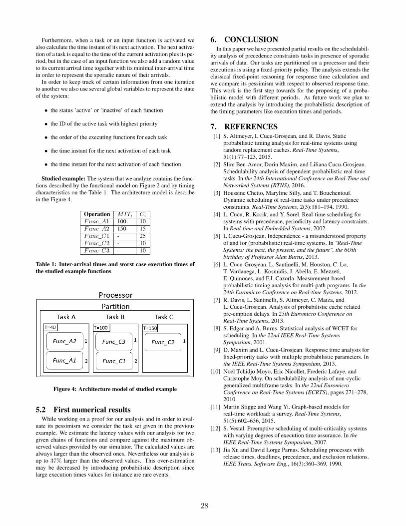
Furthermore, when a task or an input function is activated wealso calculate the time instant of its next activation. The next activa-tion of a task is equal to the time of the current activation plus its pe-riod, but in the case of an input function we also add a random valueto its current arrival time together with its minimal inter-arrival timein order to represent the sporadic nature of their arrivals.
In order to keep track of certain information from one iterationto another we also use several global variables to represent the stateof the system:
• the status ’active’ or ’inactive’ of each function
• the ID of the active task with highest priority
• the order of the executing functions for each task
• the time instant for the next activation of each task
• the time instant for the next activation of each function
Studied example: The system that we analyze contains the func-tions described by the functional model on Figure 2 and by timingcharacteristics on the Table 1. The architecture model is describein the Figure 4.
Operation MITi Ci
Func_A1 100 10Func_A2 150 15Func_C1 - 25Func_C2 - 10Func_C3 - 10
Table 1: Inter-arrival times and worst case execution times ofthe studied example functions
Figure 4: Architecture model of studied example
5.2 First numerical resultsWhile working on a proof for our analysis and in order to eval-
uate its pessimism we consider the task set given in the previousexample. We estimate the latency values with our analysis for twogiven chains of functions and compare against the maximum ob-served values provided by our simulator. The calculated values arealways larger than the observed ones. Nevertheless our analysis isup to 37% larger than the observed values. This over-estimationmay be decreased by introducing probabilistic description sincelarge execution times values for instance are rare events.
6. CONCLUSIONIn this paper we have presented partial results on the schedulabil-
ity analysis of precedence constraints tasks in presence of sporadicarrivals of data. Our tasks are partitioned on a processor and theirexecutions is using a fixed-priority policy. The analysis extends theclassical fixed-point reasoning for response time calculation andwe compare its pessimism with respect to observed response time.This work is the first step towards for the proposing of a proba-bilistic model with different periods. As future work we plan toextend the analysis by introducing the probabilistic description ofthe timing parameters like execution times and periods.
7. REFERENCES[1] S. Altmeyer, L Cucu-Grosjean, and R. Davis. Static
probabilistic timing analysis for real-time systems usingrandom replacement caches. Real-Time Systems,51(1):77–123, 2015.
[2] Slim Ben-Amor, Dorin Maxim, and Liliana Cucu-Grosjean.Schedulability analysis of dependent probabilistic real-timetasks. In the 24th International Conference on Real-Time andNetworked Systems (RTNS), 2016.
[3] Houssine Chetto, Maryline Silly, and T. Bouchentouf.Dynamic scheduling of real-time tasks under precedenceconstraints. Real-Time Systems, 2(3):181–194, 1990.
[4] L. Cucu, R. Kocik, and Y. Sorel. Real-time scheduling forsystems with precedence, periodicity and latency constraints.In Real-time and Embedded Systems, 2002.
[5] L Cucu-Grosjean. Independence - a misunderstood propertyof and for (probabilistic) real-time systems. In "Real-TimeSystems: the past, the present, and the future", the 6Othbirthday of Professor Alan Burns, 2013.
[6] L. Cucu-Grosjean, L. Santinelli, M. Houston, C. Lo,T. Vardanega, L. Kosmidis, J. Abella, E. Mezzeti,E. Quinones, and F.J. Cazorla. Measurement-basedprobabilistic timing analysis for multi-path programs. In the24th Euromicro Conference on Real-time Systems, 2012.
[7] R. Davis, L. Santinelli, S. Altmeyer, C. Maiza, andL. Cucu-Grosjean. Analysis of probabilistic cache relatedpre-emption delays. In 25th Euromicro Conference onReal-Time Systems, 2013.
[8] S. Edgar and A. Burns. Statistical analysis of WCET forscheduling. In the 22nd IEEE Real-Time SystemsSymposium, 2001.
[9] D. Maxim and L. Cucu-Grosjean. Response time analysis forfixed-priority tasks with multiple probabilistic parameters. Inthe IEEE Real-Time Systems Symposium, 2013.
[10] Noel Tchidjo Moyo, Eric Nicollet, Frederic Lafaye, andChristophe Moy. On schedulability analysis of non-cyclicgeneralized multiframe tasks. In the 22nd EuromicroConference on Real-Time Systems (ECRTS), pages 271–278,2010.
[11] Martin Stigge and Wang Yi. Graph-based models forreal-time workload: a survey. Real-Time Systems,51(5):602–636, 2015.
[12] S. Vestal. Preemptive scheduling of multi-criticality systemswith varying degrees of execution time assurance. In theIEEE Real-Time Systems Symposium, 2007.
[13] Jia Xu and David Lorge Parnas. Scheduling processes withrelease times, deadlines, precedence, and exclusion relations.IEEE Trans. Software Eng., 16(3):360–369, 1990.
28

