1

Problem Set 1 "Working with the Solow model"

Let's define the following exogenous variables:

s = savings rate

δ = depreciation rate of physical capital

n = population growth rate

L = labor supply = ent (Normalizing labor supply per capita and time 0

population to unity )

x = rate of growth of labor augmenting technology.~L = effective labor supply = e(n+x)t

and the following endogenous:~k = capital stock per effective labor unit (K/

~L ).

~y = output per effective labor unit (Y/~L ).

k = capital stock per capita

y = output per capita

1.

a)What is the growth rate of ~L . If

~k grows at rate γ (i.e., ~� /

~k k = γ ), what is the growth

rate of k, K and ~k α . What is a proper unit of γ ?

b) The gross resource constraint for a closed economy can be written

sF K L( ,~

) = Gross Investment (1.1)

How should we define gross investment? Substitute your definition into (1.1) and thensubstitute a Cobb-Douglas production function (Y= K Lα α~1− ) for F. Use this to derive, step

by step, an expression for the growth rate of ~k . (Hint: Divide by ~L , then calculate

~�

k by

noting that ~�

~kt

K

L= �

�����

∂∂

, and you get and expression containing �

~K

L. Then substitute and

your done).

c) Provide some reasonable values for s, δ, n and x.

d) Find the steady state level of ~k , ≡ ~*k . Use your parameter values from c) to find the

steady state capital output ratio K/Y? If this ratio is constant what does it imply for the

growth rates of K and Y. Is the labor output ratio also constant?

e) In steady state what is the growth rate of GDP and of wages? What about the interest

rate, i.e., the marginal product of capital?

Problem Set 1 Macro 1994 2

2.

Barro and Sala-i-Martin make a log-linear approximation to the growth rate of ~k around

it's steady state (equation 1.31). They write:

~�

~ log~

~*

k

k

k

k= −

�

���

��β (1.2)

where

β α δ= − + +11 61 6x n (1.3)

a) Starting from steady state, if you decrease the capital stock by 1%, what is a good

approximation (no exact answers please) for the growth rate of ~k . How much is it given

the parameter values in your answer to the previous question?

b) Assume that from an initial steady state, a devastating war leads to a reduction in ~k to

one half of its steady state value. Calculate the output gap (�Y/Y*-1) immediately after this

shock. What is now the growth rate of ~k and of K, given the approximation in (1.2)?

Calculate the change in interest rate. Is it reasonable?

c) How big is the output gap after one year and after 10 years? Can you calculate the time it

takes until half the output gap is gone? Is this slow or fast, do you think? When is the gap

totally gone. (Hint, define the variable d k k≡ log~

/~*3 8 . What is the interpretation of d?

Compute �d from its definition. Substitute into (1.2) and you get a very simple differential

equation that you can solve explicitly.)

d) If you increase α what happens to the rate of convergence and to the steady state capital

stock. What do you think happens as α approaches 1.

Voluntary extra question

Use the exact solution to the differential equation for ~k given in footnote 15 in Barro and

Sala-i-Martin to see how far off the log-linear approximation is for some reasonable

parameter values.

1

Problem Set 2"The Ramsey Model for an Open Economy

with Imperfect Markets"

This problem extends the standard Ramsey model you saw in class. Before you do the

problem, compare this model to the Solow model in terms of model assumptions. Do they

address the same questions? When is which model more useful?

Assumptions

We use the same notation as in Problem Set 1. For simplicity we set x and n to 0. This

means that we don't have to worry about the differences between per capita, per effective

labor unit and aggregate units. We are now looking at an open economy. The firm sells its

good on the world market but it faces a downward sloping demand curve. The price P of

the firm's output is a negative function of how much it produces. The good that it produces

cannot be stored so everything the firm produces has to be sold immediately. The firm buys

capital from abroad at a price Pk. There is, however, an imperfection in the international

transportation sector. The more capital the firm buys per unit of time, the more expensive

transportation becomes. Households buy consumption goods a a perfect world market at

price 1.

Firms

Technology and demand are given by

y kP P y

t t

t t

==

α( ).

(2.1)

To invest at the flow i the firm has to pay iPk(1+T(i)) per unit of time. T(i) is the transpor-

tation cost and T'(i)>0 for i>0. The firm also has a fixed number of employees and pays w

in wages to them. The firm pays its profits to the household in the form of dividends, dt. It

maximizes the present value of dividends and thus solves

max ( ) ( ) ,

�

i

rtt t t k t

t t

t t t

t

e P y y i P T i w dt

y k

k i k

k k

< A2 74 8

0 0

0

1∞

−∞

I − + −

== −=

%&K

'K

s.t.

αδ

(2.2)

John Hassler Macro, 1994 2

Since the country is small and open the interest rate, r, is given and constant. There is also

access to a perfect capital market for both firms and households.

Households

Households own the firms and supply one unit of labor inelastically. The representative

household solves:

max/

,

�

lim

/

c

t t

t t t t

t

rtt

t

ec

dt

a w d ra ca a

e a

< A0 0

1 1

0

1 1

0

∞

−∞ −

→∞

−

I −

�

��

�

��

= + + −=

=

%

&KK

'KK

ρσ

σ

s.t.

(2.3)

Questions

1.

a) Is the total cost of investing, iPk(1+T(i)), convex or concave in i for positive i? What

does that imply for the relative cost of volatile and smooth investment plans?

Solve the maximization problem of the firm in the following steps.

b) Set up the current value Hamiltonian. Represent the solution as two differential

equations, one for kt and one for qt, the current value shadow price of capital and an

investment function i=i(q,Pk).

c) Make a linearisation of the system around the steady state. For what could you use this

linearisation? When can it be dangerous?

d) From now on assume that the price functions have the following simple structure

P yy

T ii

( )

( )

= −

=

12

2

β

γ (2.4)

Solve for the steady states of kt and qt, (k* and q*) and draw a phase diagram.

John Hassler Macro, 1994 3

2

Solve the problem of the household.

a) Start by setting up the Hamiltonian, now in present values for a change. Take time

derivatives of Hc=0 and substitute in from the equation for Ha. This gives you a nice dif-

ferential equation for ct.

b) What happens if ρ ≠ r ? Is that reasonable? What is the interpretation of σ? How does

things change with changes in σ.

c) Solve for the level of ct using the transversality equation in (2.3) (Hint; present value of

consumption equals present value of income plus starting wealth).

3.

Suppose r=ρ and that the economy is in steady state. Use the phase diagram to see what

happens dynamically if we get a permanent negative shock to the demand for export goods (

β increases). What happens to consumption and the current account over time. (Hint; use

the following version of the inter temporal budget constraint:

c w d ra

c P y y i P T i ra

p p p

p p p pk

= + + ⇒= − + +

0

01( ) ( )1 6(2.14)

where superscript p denotes permanent values, defined by:

x e dtx

rx e dtp rt

p

trt

4 9 2 70 0

∞−

∞−I I= ≡ (2.15)

The present discounted value is the same as for the actual path of xt. Now write the equa-

tion for the current account, where b equals the stock of debt to the rest of the world.

− = − + − −� ( ) ( )b P y y i P T i c rbt t t t k t t11 6 (2.16)

Substitute (2.14) into the equation for the current account and note that a=-b, (the

household cannot sell its ownership of the firm and the value of the firm is not included in

a).Using this for t=0 we can then write the useful equation:

− = − − + − + − −� ( ) ( ) ( ) ( ) ( )b P y y P y y i P T i i P T i c ct tp p

t kp

kp p

4 9 1 6 4 94 91 1 0 (2.17)

Equation (2.17) can be used to intuitively derive what happens dynamically after the shock.

John Hassler Macro, 1994 4

4.

What happens if the shock is i ) temporary (happens at t=0 and ends at t=s) and; ii ) antici-

pated permanent (the information about the shock arrives at t=0 and the actual shock hap-

pens at t=s).

(Hint. Draw the phase diagrams and note that k can newer jump (why?) and that q can jump

only when new information (like information about a future productivity shock) arrives. In

the case of the anticipated shock note that at the time of the shock the phase diagram shifts

and that at exactly the time of the shift we have to be at the stable saddle path for the sys-

tem not to explode. So when the information arrives at t=0, the "old" phase diagram con-

tinues to hold. Now q jumps so that {q,k} hits the new stable path at exactly t=s).)

John Hassler, Macro 1994 1

Problem Set 3Endogenous Growth

Problem 1 Learning by Doing in a Two Sector Model

Consider a closed economy with a fixed number of people - normalized to one. The people

get utility from two sources; by being taken care of by people employed in a service sector

and from a good produced in a manufacturing sector. The instantaneuos utility function is

U s ct t t= +log( ) log( ) (3.1)

Where st is the number of hours of service per unit of time and ct is the consumption of

manufactured goods per unit of time. The individuals maximize future utility under a budget

constraint;

U e dt

s tP c s w

tt

t t t t

0

∞−I

+ =

ρ

. .,

(3.2)

where Pt is the price of manufactured goods, wt is the wage and we fix individual labor

supply to unity and normalize the price of services to unity. People can choose to work

either in the service sector or in the manufacturing sector. Labor markets and consumption

markets are competitive. Production in the manufacturing sector equals consumption and is

given by

c A lt t c= (3.3)

where At is the level of productivity and lc is the share of people working in the

manufacturing sector. Each firm takes the level of productivity as given. There is learning

by doing in the manufacturing sector, however, so A evolves over time according to:

�A ct t= υ (3.4)

Questions

a) Before doing any number crunching think about the following. In this economy, what will

happen to the future consumption possibility set if all people decide to consume more

manufactured goods today? If only one person consumes more manufactured goods? What

do you think of the specification of learning by doing, does it make sense?

John Hassler, Spring 1994 2

b) When we normalize the price of services to unity what is the wage rates in the two

sectors?

c) With perfect competition in the manufacturing sector what is the price of manufactured

goods?

d) Solve the maximization problem of the consumer. (Hint: All individuals are equal. This

implies that if there is a capital market the interest rate will have to adjust so that no one will

borrow. We can thus as well assume that there is no capital market. The maximization

problem of the consumer is the static.)

What is the growth rate in this sector. What happens to the growth rate if more people

work in the manufacturing sector?

f) Now let's find the optimal amount of people in the manufacturing sector. First, do you

think it should be higher or lower than the market solution?

To find the solution, follow these steps:

1. Let there be a benevolent central planner who maximizes the individuals' utility but takes

into account the learning by doing effect. Assume there is no possibility to store the

manufactured good.

2. Write the Hamiltonian and the optimality conditions. Note how the Hamiltonian differs

from the static problem of the individual. Guess that in an optimal steady state, the labor

shares are constant and then differentiate the first optimality condition (Hl) w.r.t. time.

What is then the relationship between the growth rate of the shadow value of the

constraint and the growth rate of A? Eliminate the growth rate of the shadow value and

the shadow value from the second optimality condition (HA) and you get an expression

for the growth rate of A involving υ, lc and ρ

4. There is another expression for the growth rate of At coming from the learning by doing

constraint. Use this to eliminate the growth rate of At.

(3.4)Problem 2. The "School is Never Out" – model

There is a continuum of workers-consumers on the interval [0,1], i.e. an infinite number of

agents indexed by the real numbers i between 0 and 1. Each individual i has one unit of

labor to spend per day (rather per instant). Since all individual are alike we can drop the i

superscript where we don't need it. Her decision is how much of the day to spend in school

(1-ai) and how much to work (ai). She can, however, never quit shool. When she goes to

school she accumulates human capital (hi) at a rate proportional to the time spent in school.

� ( )h a ht t= −β 1 (3.12)

John Hassler, Spring 1994 3

The interesting thing with the model is that the productivity of individual i depends on the

human capital of everybody else. By working with smart people your productivity increases.

The production of a single individual is thus given by:

y ah AHt t t=−

2 7 2 7α α1

(3.13)

Where A and H denotes aggregate levels of a and h.

H h di

A a di

t ti

t ti

=

=

I

I

0

1

0

1(3.14)

The production cannot be stored, so the individual consumer-producer consumes what she

produces each moment in time so she solves

max log( )

. .

� ( )

a tt

t t t

t t

y e dt

s t

y ah AH

h a h

h h

0

1

0

1

∞−

−

I

== −=

ρ

α α

β2 7 2 7 (3.15)

Questions

a) Is there decreasing or constant returns to human capital in this model? How much of the

externality is taken into account by this small selfish agents? This can be found be evaluating∂∂

H

hi.

b) Assume a common value of a for all agents, (is this reasonable?), then compute the

growth rate of the economy as a function of a.

c) Derive the equilibrium growth rate of the economy by letting the agents choose a

optimally. (Hint; Set up the maximization problem of the consumer-producer and substitute

for c in the utility function. Set up the Hamiltonian with its optimality condition and the

solve for the growth rate of human capital assuming a steady state where a is constant.

d) Derive the optimal growth rate of the economy. Can you explain your results?

John Hassler, Spring 1994 4

Appendix to P-Set 3 Regarding continuous populations

A continuous population is surely an abstraction. If we index people with all rational

numbers between 0 and 1 each have to be infinitely small, e.g., have zero human capital in

order for aggregate human capital to be finite. Nevertheless this may be a useful abstraction.

To try to give some intuition, look at a population consisting of N (where N is very big)

individuals. To calculated their aggregate human capital we can divide the population into I

groups of equal size, indexed by i = {1,...I}. Then we figure out the average level of human

capital per capita in each group,hiI . For higher I we get a finer division of the population

and for each I we choose we get a sequence of hiI for i = {1,...I}. I have drawn two figures

of hiI for I = 5 and 25 below. Note that if we increase I, hi

I will change for each i but it

will keep its approximate order of magnitude constant.1

0

0.1

0.2

0.3

0.4

0.5

0.6

0.7

0

0.1

0.2

0.3

0.4

0.5

0.6

0.7

0.8

0.9

1

1 In the sense that the average over all i remains constant when I increase but the variance increases.

John Hassler, Spring 1994 5

The amount of human capital in each group is then:

N

Ihi

I , (3.23)

So to get total human capital we sum over the groups:

HN

Ih

i

I

iI=

=∑

1

(3.24)

This is equal to the are of all the bars in the figures, noting that the base of each bar is N/I.

We can also compute how much an increase in the average human capital level for one

group i affects aggregate human capital. It is going to be:

dH

dh

N

IiI

= (3.25)

Thus we see that:

dH

dh

N

IiI

= (3.26)

decreases when I increases (the partition becomes finer). Suppose we increase I very much,

sooner or later then N=I . After that we cannot go on in reality since then we have to start

splitting people (we could in fact divide people into parts and let the parts share equally the

human capital of the individual, in this case it doesn't, however, make much sense to think

of increasing the human capital of a part of an individual). On the other hand, if N is large

we can increase I very much before we run into this problem and we may be forgiven if we

forget that constraint. If we the let I go to infinity we have:

lim

lim lim

Ii

I

iI

iI

IiI I

NIh N h di

dH

dh

N

I

→∞=

→∞ →∞

∑ I�

���

�

���

=

= =

1

0

1 0

1

(3.27)

In some cases, like the one in P-set 3, it is much easier to do calculations with I going to

infinity. Then we may formally disregard the externality when optimizing for the individual.

For I large but finite this is only on approximation. Nota bene the connection to small firms

and perfect markets.

John Hassler, Macro 1994 1

Problem Set 4The Overlapping Generations Model

Question 1.

Consider an overlapping generations model in discrete time, where people work and earn a

wage wt in the first period and are retired consuming their savings st plus interest in the

second. A generation born at time t consumes ct when young and dt+1 when old. They thus

solve the problem:

max ( ) ( ) ( )

. .( )

,c d t t

t t t

t t t

t t

U c U d

s t c s wd s r

+

+ +

+ == +

−+

+ +

1

1

1

11

1 1

θ4 9(4.1)

All variables are per capita which is taken to mean that we divide with the size of the

relevant generation. There is production with constant returns to scale. Perfect markets

ensures that:

r f kw f k r kt t

t t t t

== −

' ( )( )

(4.2)

The savings in period t constitutes the capital for the next generation to work with in period

t+1. The population grows at rate n so

k n st t+ + =1 1( ) (4.3)

1.

a) Show that indirect utility increases in wt and rt+1.

b) Solve the problem of the consumer for a general utility function. Express your result as a

savings function only depending on kt, kt+1 and parameters. Give me an equation that

implicitly defines a steady state.

c) Can we say anything about the stability of the steady state?

2.

Now assume logarithmic utility. Find a savings function. Show that it does not depend on

kt+1 and explain why.

John Hassler, Spring 1994 2

3.

Now also assume Cobb-Douglas production so

f k k( ) = α . (4.8)

Use the savings function to get a difference equation which you solve for a steady state and

find a condition for stability.

4.

Now let's use this model to study the effect of a budget deficit used to finance transfers to

the current tax payers, i.e., the current situation in Sweden. According to the Ricardian

Equivalence Theorem by Barro, such a policy should have no effect. But what is the

predictions of this model? Let's formalize the question as follows. The government borrows

bt at time t from the currently young. The receipts are immediately paid back to the

currently young as transfers. The government is not allowed to go bankrupt so in t+1 the

old get back what the government borrowed plus interest.

a) First assume that next generation restores the government's financial position by paying

back bt(1+rt+1) to the old. Write down the budget constraints for the young in t and t+1.

Find the sign of the effects on capital stocks, wages and utility for the generations born in t

to t+2 for a small bt and starting from a steady state.

b) Now assume that the generation born in t+1 and onwards pays interest but rolls over the

principal by letting the government borrow to finance paying back the principal to the old.

Write down the budget constraints for the young in t and t+1. Find the sign of the effects on

capital stocks, wages and utility for the generations born in t to t+2 for a small bt and

starting from a steady state.

c) Assume that the generations born from t+1 and onwards roll over all debt including

interest rates. How will bs evolve for s>t? What happens if rs<n? Explain.

John Hassler, Spring 1994 3

Appendix to P-Set 4

A Simple Example with Death Probability

Here is an example that shows that it is not the chance of death but rather the birth of new

generations that breaks Ricardian Equivalence in an overlapping generations model. Let's

assume that there is a probability to die which is 1-p, that r=φ=0, and that there is a perfect

capital market so if one saves and don't die one gets a return of 1/p on the savings. In

addition n individuals are born in period 2. The individual in period 1 then maximizes

max

. .

,c cU c pU c

s t cw c

p p

1 21 2

21 1

2

2 7 2 74 8+

=−

− −τ

τ

The budget constraint for the government is then

G p n= + +τ τ1 2( ) .

In the second period there are p people around, so the tax receipts are pτ2. Then a balanced

tax shift satisfies

∆ ∆ ∆ ∆τ τ τ τ1 2 1 20+ + = ⇒ = − +( ) ( )p n p n

Substitute this into the budget constraint of the individual and we get

cw c

p pw c

p

p n

pw c

p p

n

p

21 1 1

2 2

1 1 22 2

1 12 2

=−

−+

− +

=−

−+ − +

− +

=−

− − +

τ ττ τ

τ ττ τ

ττ τ

∆∆

∆∆

∆

( )

( ( ) )( )

So the chance to get away with some tax payments is exactly balanced by that higher taxes

have to be paid if one survives if n=0. I.e., expected tax payments are then independent of

the death probability. If, on the other hand, n>0 the consumption possibility set is increased

if taxes are shifted forward in time.

John Hassler, Macro 1994 1

Problem Set 5Consumption under uncertainty

Question 1.

Consider a person who lives for two periods and has the same utility function in both

periods but discounts utility in the second with 1+θ. She faces a constant interest rate r and

her income in period one is y1. In period two her income ~y2 is random with mean y2. She

maximizes expected utility seen from period 1.

1.

Define the maximization problem of the consumer and show that the first order condition is

U cr

E U c' ( ) ' ( )1 2

1

1= +

+ θ2 7 (5.1)

where E defines the expectations operator.

Will equation (5.1) be satisfies also in a multi-period model? (If you can, define a value

function and use it to prove the answer. Otherwise make an informed guess and provide

some heuristic arguments.)

2.

Now assume quadratic utility

U cc= −α β 2

2. (5.6)

Find the FOCs. Solve for the consumption c1 of the consumer. How does the consumption

depend on the degree of income risk? Explain your result and discuss the usefulness of this

utility specification.

3.

Using the quadratic utility function, let's do a Hall-type consumption time series regression.

c ct t t= + +−µ φ ε1 (5.8)

What is the true regression coefficient I? Estimate the parameters of the regression from

Swedish consumption data. Discuss potential problems and remedies in OLS estimation.

John Hassler, Spring 1994 2

Include more RHS variables that are known in period t-1, e.g., ct-2? Do your result accord

with the theoretical predictions?

4.

Now let's look at some other utility functions. First let the individual have the following

utility function.

U ce c

( ) = −−α

α(5.11)

Find the degree of absolute risk aversion of this individual.

Now, set for simplicity r and T to zero. Let the second period risk be additive and normally

distributed so that

~ , ,y y N2 220= + =ε ε σd 4 9 (5.12)

Solve for c1. Hint; Remember the following relation:

x N x

E e e

x

x x x

=

⇒ = +

d,

/

σβ β β σ

2

22 2

4 9(5.13)

Define precautionary savings, s(V), as the difference between consumption with no risk and

with risk.

s c c( )σ σ≡ = −12

104 9 . (5.14)

Is precautionary savings increasing in the variance and D? Is it increasing in income?

5.

Now let

U cc

( ) =−

−1

1

α

α(5.17)

Find the degree absolute risk aversion of this individual, how does it depend on

consumption?

John Hassler, Spring 1994 3

To get analytical solution to this problem we need multiplicative risk that is log-normally

distributed, i.e., we may think of risk as a risky return and that the percentage return has a

normal distribution. So

c y y c

N

2 1 2 1

20

= + −

=

2 7

4 9

ε

ε σlog ,d

(5.18)

where y2 is known in the first period.

Solve for c1. Hint; log(c2) is normal so you can use the hint to the previous question.

Now define relative precautionary savings as

sc

cr ( )σ

σ≡ −

=1

01

12

(5.19)

Is relative precautionary savings increasing in the variance and D? Is it increasing in income?

Which of the two utility functions you have worked with do you think captures attitudes

towards risk best?

John Hassler, Macro 1994 1

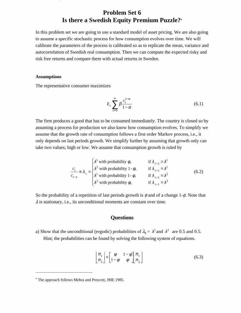
Problem Set 6Is there a Swedish Equity Premium Puzzle?*

In this problem set we are going to use a standard model of asset pricing. We are also going

to assume a specific stochastic process for how consumption evolves over time. We will

calibrate the parameters of the process is calibrated so as to replicate the mean, variance and

autocorrelation of Swedish real consumption. Then we can compute the expected risky and

risk free returns and compare them with actual returns in Sweden.

Assumptions

The representative consumer maximizes

Ec

tt

s

βα

α1

01

−

=

∞

−∑ (6.1)

The firm produces a good that has to be consumed immediately. The country is closed so by

assuming a process for production we also know how consumption evolves. To simplify we

assume that the growth rate of consumption follows a first order Markov process, i.e., it

only depends on last periods growth. We simplify further by assuming that growth only can

take two values; high or low. We assume that consumption growth is ruled by

c

ct

tt

t

t

t

t

−

−

−

−

−

≡ =

====

%

&

KK

'

KK

1

11

1

21

1

11

2

21

2

λ

λ φ λ λλ φ λ λλ φ λ λλ φ λ λ

with probability if

with probability 1- if

with probability 1- if

with probability if

,

,

,

,

(6.2)

So the probability of a repetition of last periods growth is I and of a change 1-I. Note that

O is stationary, i.e., its unconditional moments are constant over time.

Questions

a) Show that the unconditional (ergodic) probabilities of Ot = λ1and λ2 are 0.5 and 0.5.

Hint; the probabilities can be found by solving the following system of equations.

ππ

φ φφ φ

ππ

1

2

1

2

11

�

!

"

$# =

−−

�

! "

$#�

!

"

$# (6.3)

* The approach follows Mehra and Prescott, JME 1985.

John Hassler, Spring 1994 2

where the S's are the wanted probabilities. Try to understand why these equations give you

the unconditional probabilities.

b) Parameterize by setting

λ µ δλ µ δ

1

2

1

1

= + −= + +

(6.4)

Show that the unconditional mean, variance and autocorrelation of Ot are

1 2 12+ −µ δ φ, ,> C . Hint; Use the relation

E m E m E mt t t t t= = + =− −λ λ π λ λ π11

1 12

2 (6.5)

where mt is the moment you are looking for.

c) Estimate the sample mean, variance and autocorrelation of Ot from the Swedish data on

consumption. Use the results calibrate the model, that is to assign numbers to µ δ φ, ,; @ .

Now we can also compute the process for the price of the firm in the model. The price will

generally depend on the current level of consumption and on expectations about future

consumption growth. With the simple Markov process for consumption, expectations only

depend on last periods growth. Furthermore the CRRA utility function implies that the price

is homogeneous of degree 1 in the current level of consumption. This means that the price

of the firm only depends on current consumption and on last periods growth, and that it is

linear in current consumption. Let P(c,O) denote the price of the firm. We can then write

standard pricing function for assets as

P c p c EU c

U cp c c

P c p c EU c

U cp c c

t t tt

t

it t t

t t tt

t

it t t

,

,

λ β λ λ

λ β λ λ

1 1 11 1

1

2 2 11 1

2

4 92 72 7 4 9

4 92 72 7 4 9

≡ =′

′+ =

�

!

"

$##

≡ =′

′+ =

�

!

"

$##

++ +

++ +

(6.9)

pi can now be interpreted as the price of the firm relative to the current level of consump-

tion, given that the growth from last to current period was Oi.

d) Divide both sides of the pricing function with ct, substitute to get rid of ct and ct+1.

Derive a two equation system that (implicitly) defines pi in terms of {E, I,O1,O2,D}.

e) If Ot=Oi and Ot+1 happens to be Oj, the return on equity from t to t+1 can be written

John Hassler, Spring 1994 3

~rp c c p c

p cij

jt t

it

it

=+ −+ +1 1 (6.13)

Get rid of consumption in the last equation and derive an expression for the unconditional

expected return on equity.

Plug in the estimated values of µ δ φ, ,; @ and set E = 0.95 and D = 1,5 and 10. Compute the

unconditional expected return on equity.

f) Show that the unconditional risk less rate of return equals

Er =+ −�

���

++ −�

���

−− − − −

1

2 1

1

2 11

1 2 2 1β φ λ φ λ β φ λ φ λα α α α

4 9 1 64 9 4 9 1 64 9(6.16)

g) Compute the models predicted equity premium for the three different risk aversion

coefficients.

h) Estimate average real return on equity and on bonds from the Swedish financial data.

What is the average equity premium in the sample?

i) Compare the sample equity premium with the predictions of the model. What do you

conclude?

John Hassler, Spring 1994 4

John Hassler, Spring 1994 5

John Hassler, Macro 1994 1

Problem Set 7A Simple Real Business Cycle Model*

In this problem set we are going to construct a small real business cycle model and use

Swedish data to calibrate it. Since it is very simple it may not perform perfect but it will

illustrate the main ideas and virtues of this kinds of models. RBC models have some typical

features;

� They build on maximizing agents.

� A maintained hypothesis is that real shocks drive the business cycle.

� They try to model a propagation mechanism such that a simple shock, typically

technological, can cause persistent business cycles.

� Parameter values are as far as possible taken from other "usually reliable sources"

(which in this case will be my pure guesses).

� They choose the rest of the parameter values so that the model replicates some interest-

ing moments of aggregate macro variables, typically relative standard deviations, corre-

lations and autocorrelations. Often the models are analytically unsolvable so the model

moments are generated by simulation.

Constructing the Model

Let there be representative consumer with log utility who owns a firm with CD technology.

At time t the problem for the consumer is then

max ln

. .

E C

s t C K Y

Y Z K

ts

s t

s

t t t

t t t

β

α

+=

∞

+−

∑+ ==

2 70

11

(7.1)

Where Zt is a technological shock that we will specify later. Necessary conditions for an

optimal solution is that

1

1 1 1 1

11

C

E Z K

C K Z K

tt

t t t t t

t t t t

=

= −+ =

+ + +−

+−

Λ

Λ Λα β α

α1 6 (7.2)

where / is a shadow value.

* The approach follows McCallum, 1989, in Modern Business Cycle Theory.

John Hassler, Spring 1994 2

a) Write down a verbal interpretation of each of the necessary conditions.

Now we will try to find one of the possibly infinite solutions and hope that one satisfies the

transversality condition. If so, the solution also satisfies sufficient optimality conditions.

First we start by guessing that consumption is proportional to production, with propor-

tionality 3 so that

C Z Kt t t= −Π 1 α (7.3)

b) Find Kt+1 as a function of 3, Zt and Kt.

c) Show that if our guess is correct

Π = − −1 1 α β1 6 (7.4)

Hint. Use first the optimality condition to eliminate / in the second. Then use the guess and

your answer to b).

From now on we use lower case letters to indicate logs and we assume that the log of the

technology shock is white noise. We can now establish that

k k z

c c z

y y z

t k t t

t c t t

t y t t

+

−

−

= + − += + − += + − +

1

1

1

1

1

1

π απ απ α

1 6

1 6

1 6

(7.5)

where

πππ α π

k

c

y k

= −== −

loglog( ) log

1

1

ΠΠ1 6

(7.6)

d) Is the solution satisfying the transversality condition that

limj t

jt j t jE K

→∞ + + + =β Λ 1 0? (7.7)

e) Using (7.5) it is possible to show that this very simple model gives us perfectly correlated

series for k, c and y. Can you think of a way to break this?

John Hassler, Spring 1994 3

Calibration

Take the following parameter as given from "usually reliable sources" E = 0.95. We now

have two parameters left; the variance of zt, defined as σ z2 and D. These are going to be

chosen so as to match the variance and autocorrelation of consumption.

a) Detrend consumption data by regressing the log of ct on a constant and a time trend.

Define the residuals as the business cycle component. Calculate the variance and

autocorrelation of the consumption business cycle, σ c2 .

b) Use a computer to simulate the model. Generate a series of normally distributed shocks

of suitable length. Generate simulated series for a few values of σ z2 in the range from σ c

2 /5

to σ c2 and for D in the range 0.1 to 0.7. Include at least the four combinations of endpoints.

Set the first observations on simulated c to π αc / . Then choose the set of parameters that

gives you the best match between simulated and sample moments. This is the end of the

calibration.

Simulation

Now we have all the necessary parameters so we can see if the model is able to generate

simulated series with statistical properties similar to data.

a) Simulate the model. Plot the result including the shocks. Also plot the business cycle of

ct. See if you can find some similarities and differences.

c) Compute the autocorrelation for 1,2, and 3 lags in the sample and in the simulated data.

d) Discuss the model's performance and what you think could be done to improve it.

John Hassler, Spring 1994 4