i. endogenous growth in the generalized solow model 1 of 18 the generalized solow model with ......
TRANSCRIPT

Page 1 of 18
The generalized Solow model with endogenous growth
December 2015
Alecos Papadopoulos
PhD Candidate
Department of Economics
Athens University of Economics and Business
This sprung out of the Graduate Macro I class 2015-2016. I decided to elaborate on a
short section of the main textbook's chapter on Endogenous Growth models, in order to clarify
the properties of the long-run equilibrium, the issue of transitional dynamics in endogenous
growth models, and how one can simulate them.
I. Endogenous Growth in the generalized Solow model
"Solow" growth model implies that the investment rate(s) are fixed."Generalized"
Solow model means that both physical and human capitals are present. The model was
introduced by Mankiw et al. (1992) in order to enhance the basic Solow model of growth so
that it fits better the available data. In their version growth was not endogenous. Specifically
they considered a model of the form
1
( ) ( ) ( ) ( )aY t A t L tK t
1
( ) (( ) ) ( ), ) (gth t h t ta e H Lt t
0 1
,K KK s Y K H s Y H
where notation should be obvious. gte is the exogenous technical progress term that
augments the efficiency of labor, with its initial level normalized to unity, and we also

Page 2 of 18
assume that population ( )L t grows at constant rate n . The initial values of technical
progress and labor are normalized to unity.
When 1 the production functions exhibits constant returns to scale in , ,K H L :
1
1 (1 )(1 )(1 ) (1 )(1 )( ) ( ) ( )( ) ( ) ( ) ( ) ( )gt gtY t AK t H t L t AKe L t H t L t et
In fact this is the critical issue as to whether the model will exhibit capability for
endogenous growth or not. If you see an abstract production function , ,F K H L for which
it is assumed that , , , ,F K H L F K H L , i.e. constant returns to scale in all three
factors, then the per capita production function
, ,1 ( , )Y LF K L H L Y L y f k h
will exhibit diminishing returns to scale in ,k h and the model won't be capable for
endogenous growth (so such an abstract formulation is equivalent to assuming 1 ). If
exogenous technical progress exists, the per capita magnitudes will grow but only because of
it.
We are interested in the "endogenous growth" case, for which we need to impose 1
. Here, the term gte disappears from the production function. If you want to be very
pedantic, 1 does not imply that labor efficiency is fixed: we have every right to assume that
labor's "productive potential" is increasing but somehow, it does not find its way into the
production function, and so it does not contribute to output: in fact the case 1, 0g
could be used to model organizational failure: firms employ people that increase their
individual efficiency, but the production function in place (the work processes, the
organizational structure, the production system in general) fails to let this increased
efficiency produce results (leading thus to a declining output per efficiency unit and
reasonably to disappointed workers that feel that they are being wasted).
But in our model, when assuming 1 , we also assume 0g , and the only source of
exogenous growth remaining is the population growth. So at the very least, in the balanced
Page 3 of 18
growth path, total magnitudes will grow at rate n, while per capita variables will be constant.
But we want more than that. Let's see how we can get it.
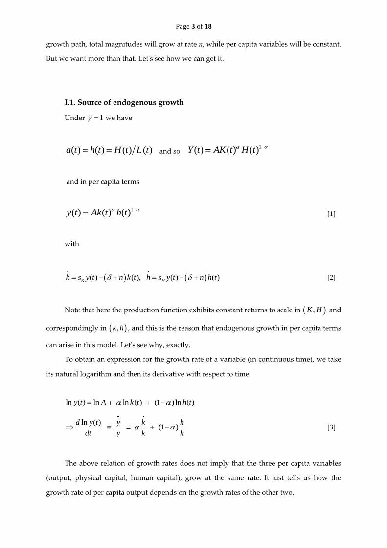
I.1. Source of endogenous growth
Under 1 we have
( ) )) ) (( (a t h t H t L t and so 1( ) ( ) ( )H tY t AK t
and in per capita terms
1( ) ( ) ( )y h tt Ak t [1]
with
( ) ( ), ( ) ( )K Hk s y t n k t h s y t n h t [2]
Note that here the production function exhibits constant returns to scale in ,K H and
correspondingly in ,k h , and this is the reason that endogenous growth in per capita terms
can arise in this model. Let's see why, exactly.
To obtain an expression for the growth rate of a variable (in continuous time), we take
its natural logarithm and then its derivative with respect to time:
ln ( ) ( )ln ln (1 )ln ( )t A k ty h t
ln ( )(1 )
d y y k h
dt y h
t
k [3]
The above relation of growth rates does not imply that the three per capita variables
(output, physical capital, human capital), grow at the same rate. It just tells us how the
growth rate of per capita output depends on the growth rates of the other two.

Page 4 of 18
From the laws of motion of the two capitals we have
( )( ) ( )
( )
( )( ) ( )
( )
K K
H H
k y tk s y t n k t s n
k k t
h y th s y t n h t s n
h h t
Inserting into the expression of the per capita output growth rate,
( ) ( )
(1 ) (1 ) (1 )( ) ( )
K H
y k h y y t y ts n s n
y k h y k t h t
( ) ( )
(1 )( ) ( )
K H
y y t y ts s n
y k t h t [4]
or alternatively
( ), ( ) ( ), ( )K k H h
ys f k t h t s f k t h t n
y [5]
Equation [5] connects the per capita growth rate of output with the marginal
products of the two capitals. We see that what we need for a constant output growth rate is
that the marginal products of the two capitals are constant (not equal).
We know that the reason for zero long-run growth in per capita terms (or in per
efficiency terms, if technical progress is positive), with only physical capital present, is the
fact that the marginal product of capital diminishes as the level of capital accumulates.
What happens in the current model is that because we have two capitals, two
accumulated factors, "the one can help the other maintain a constant and positive marginal
product", even though both their levels increase, and thus leading (possibly) to positive
growth rate of per capita output.

Page 5 of 18
I.2 Economic models and the long run growth rate
Our models should bear some resemblance with the real world, no matter how abstract
they are. The real world data tells us that a) per capita growth is observed b) it is relatively
stable, per economy, in most economies c) ratios of basic macroeconomic variables, like
consumption or capital over output, although not stable over time, they do not appear to
tend to extremes (to "zero" or to "infinity"). Our models should be able to replicate broadly
these empirical regularities (and others of course, see "stylized facts of growth").
The first empirical regularity demands from us some source of per capita growth. We
initially came up with an exogenous source (technical progress), and now we are examining
endogenous sources. The second regularity, demands that in the long-run the model leads to
these growth rates being eventually constant. The third one demands that these growth rates
are equal, at least in the long-run.
In economics speak, we codify this by saying that we need to obtain a "balanced
growth path" in per capita terms, i.e. that we need to have
0B B
k h yg g
k h y [6]
Note that the requirement that the common growth rate is positive is a separate one.
Mathematically the model does not exclude the case
0k h y
k h y
1) Equal growth rates
From (1 )y k h
y k h

Page 6 of 18
the condition for an equal growth rate for all three variables is
( ) ( )
( ) ( )
KK H
H
sk h y t y t ks n s n
k h k t h t h s [7]
Note how the constant-returns-to-scale property is critical here). Also, remember Note
that the above says only that the growth rates will be equal, not that they will also be constant
through time. And certainly, this condition does not imply that this growth rate (of the per
capita magnitudes, i.e. over and above n) will also be positive.
2) Constant (and equal) growth rate
To obtain a constant growth rate, it must be the case that it is expressed in terms of
parameters that are considered fixed. We have already obtained the expression (eq. [4])
( ) ( )
(1 )( ) ( )
K H
y y t y ts s n
y k t h t
Writing the per capita production function explicitly we have
1 1( ) ( ) ( ) ( )
(1 )( ) ( )
K H
Ak t Ay h t h ts s n
y k t
k t
h t
1
( ) ( ) (1 ) ( ) ( )K H
ys A h t s A h tk t t n
yk
[8]
Imposing the condition for an equal growth rate we have

Page 7 of 18
1
1 1
(1 )
(1 )
B K H K H K H
K H K H
g s A s s s A s s n
As s s s n
1
B K Hg As s n [9]
and now we see that the common growth rate will also be constant.
Still, the above do not imply that the growth rate will be positive.
3) Positive (as well as constant and equal) growth rate
The way to obtain a positive growth rate (that is also constant and common) for the per
capita magnitudes is simple (and unique): We assume that the values of the parameters are such
that they lead to 0Bg .
This is what "endogenous growth" models do: they allow for the possibility of an
endogenous constant and equal growth rate, and then, the parameters must be such as to
deliver it as positive also. In contrast, the standard Solow model, does not allow for
endogenous positive growth rate.
Isn't this fixing of parameters "to our liking" totally arbitrary? No, because we are doing
it in order to replicate real-world experience.
We see that the approach to solve and characterize endogenous growth models is
different. Assume that you attempted a "standard" approach, meaning, "when you see a
differential equation, put it equal to zero to see what happens". So set 0k h , and proceed from
there... you will find that in such a case, 1 0K H BAs s n g . But this only gives
us the condition on the parameters under which the per capita growth rate will be zero,
because by assuming 0k h we essentially impose a priori exactly that, so this is not a
proof that the model is such that it leads to zero per capita growth rate. Moreover, the goal of
Page 8 of 18
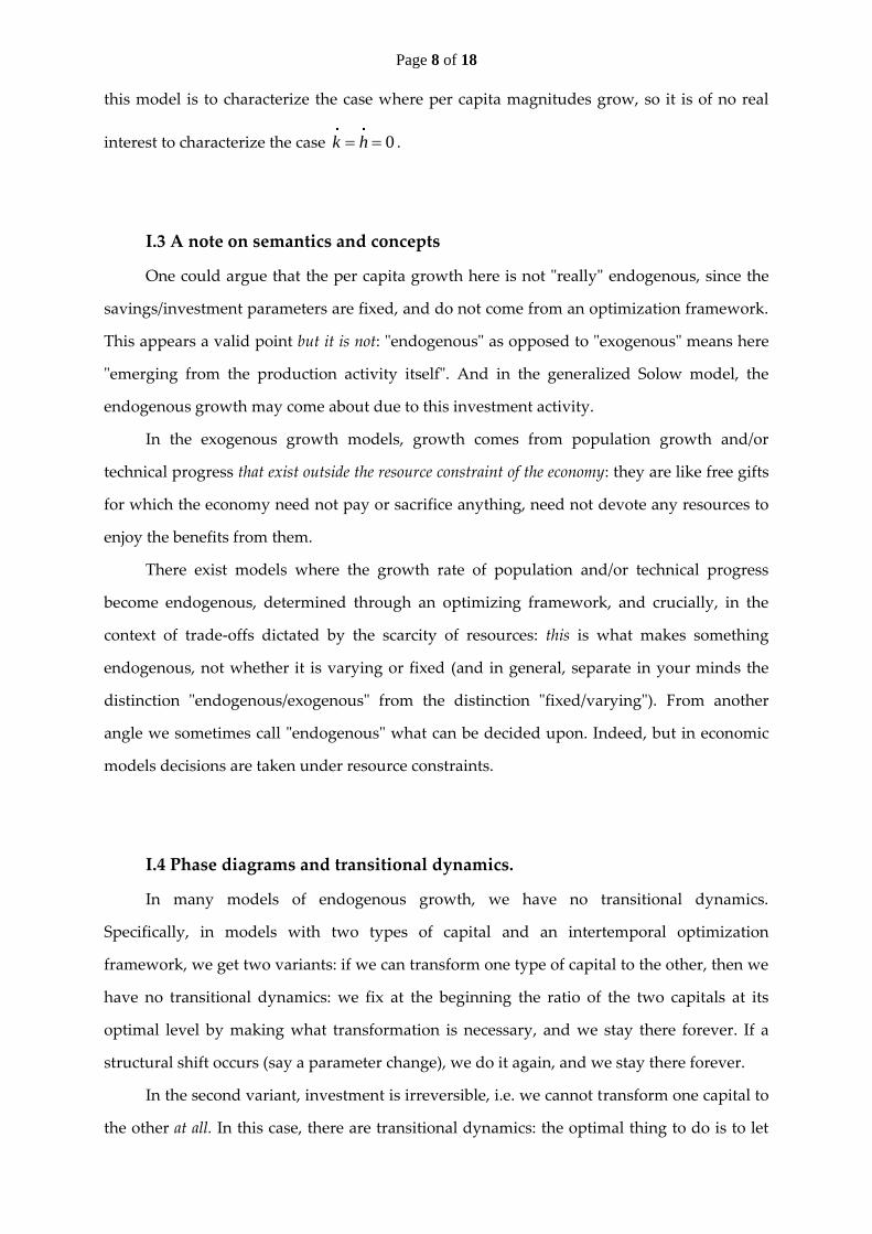
this model is to characterize the case where per capita magnitudes grow, so it is of no real
interest to characterize the case 0k h .
I.3 A note on semantics and concepts
One could argue that the per capita growth here is not "really" endogenous, since the
savings/investment parameters are fixed, and do not come from an optimization framework.
This appears a valid point but it is not: "endogenous" as opposed to "exogenous" means here
"emerging from the production activity itself". And in the generalized Solow model, the
endogenous growth may come about due to this investment activity.
In the exogenous growth models, growth comes from population growth and/or
technical progress that exist outside the resource constraint of the economy: they are like free gifts
for which the economy need not pay or sacrifice anything, need not devote any resources to
enjoy the benefits from them.
There exist models where the growth rate of population and/or technical progress
become endogenous, determined through an optimizing framework, and crucially, in the
context of trade-offs dictated by the scarcity of resources: this is what makes something
endogenous, not whether it is varying or fixed (and in general, separate in your minds the
distinction "endogenous/exogenous" from the distinction "fixed/varying"). From another
angle we sometimes call "endogenous" what can be decided upon. Indeed, but in economic
models decisions are taken under resource constraints.
I.4 Phase diagrams and transitional dynamics.
In many models of endogenous growth, we have no transitional dynamics.
Specifically, in models with two types of capital and an intertemporal optimization
framework, we get two variants: if we can transform one type of capital to the other, then we
have no transitional dynamics: we fix at the beginning the ratio of the two capitals at its
optimal level by making what transformation is necessary, and we stay there forever. If a
structural shift occurs (say a parameter change), we do it again, and we stay there forever.
In the second variant, investment is irreversible, i.e. we cannot transform one capital to
the other at all. In this case, there are transitional dynamics: the optimal thing to do is to let
Page 9 of 18
the capital that it is relatively higher than optimal depreciate (zero investment in it) for as
long as it is needed to reach the optimal capitals ratio (see Barro and Sala-i-Martin 2004, ch
5.1.1 and 5.1.2)
In the generalized Solow model with endogenous growth, there is no optimizing
framework: investment rates are fixed.
This creates the following issue: if the initial stocks of the two capitals do not satisfy the
ratio required for long-run equilibrium (eq. [7]), will the model nevertheless converge to the
steady-state? Isn't it possible, with fixed and strictly investment rates, for it to diverge?
We will show that the steady state of the model is globally stable, i.e. even if we start
with an unbalanced capitals ratio, and even if we continue investing in both capitals, we will
end up at the steady-state.
We will show this through the assumption of a structural shift in one of the investment
rates: if such a thing happens, the economy (currently assumed to be on the steady-state
given the previous set for parameter values), is now characterized by a capitals ratio that it is
not equal to the one implied by the new set of values. Still, it will converge to the new one.
This is equivalent to starting from a situation where the initial value of the capitals
ratio is not equal to K Hs s .
We need to consider issues of stability of equilibrium, and related characterizations of
the balanced growth path. Stability relates to fixed points, and to have a fixed point, one
needs variables that become constant in the long run.
An obvious approach is to use growth rates (of per capita magnitudes), and not levels
of variables. Another is to define ratios that will be constant in the balanced growth path, like
the capitals ratio.
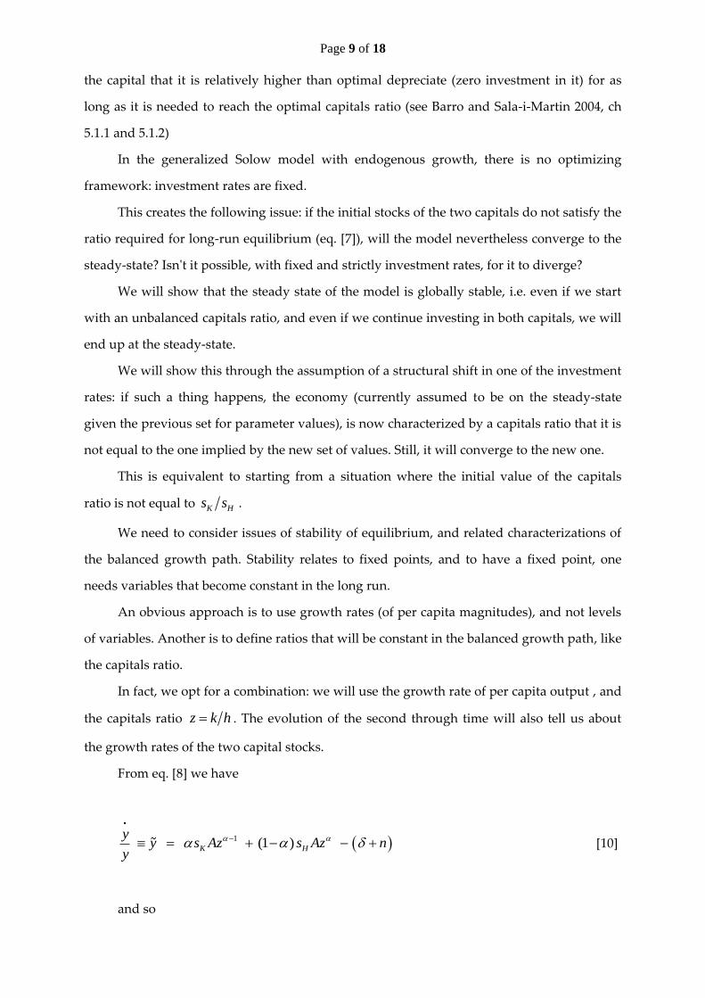
In fact, we opt for a combination: we will use the growth rate of per capita output , and
the capitals ratio z k h . The evolution of the second through time will also tell us about
the growth rates of the two capital stocks.
From eq. [8] we have
1 (1 )K H
yy s Az s Az n
y
[10]
and so

Page 10 of 18
2 1(1 ) (1 )K Hy s Az z s Az z
1 1(1 ) K Hy Az s z s z [11]
Also
1( ) ( )
( ) ( )K H K H
y t y tz z k h z s n s n z s Az s Az
k t h t
1 1
K Hz Az s z s [12]
Inserting [12] into [11] we can write
1 1 1 1(1 ) K H K Hy Az s z s Az s z s
2
1(1 ) K HAz s z s
[13]
Manipulating eq. [10]
1
1 1
(1 )
(1 )
K H
K H K H H
y s Az s Az n
y n Az s z s Az s z s s
11H K Hy n s Az Az s z s
Inserting this in [13] we get the system of differential equations

Page 11 of 18
2
1 1
(1 )H
K H
y y n s Az
z Az s z s
[14]
The zero change loci are
0
0
H
K H
y y s Az n
z z s s
[15]
Note that outside its zero-change locus, the output growth rate is everywhere
declining. So we have the following phase diagram:

Page 12 of 18
What we learn from the above phase diagram is that the output growth rate can
approach its steady-state value only from above. So in an adjustment process, if y is below
the new steady state value, we expect to see it jump up, overshooting its long-term value,
and then to decline.
We turn now to consider structural shifts in the form of an increase in the investment
rates.
I.4.1 An increase in the rate of investment in physical capital Ks
An increase in Ks moves the 0z locus to the right, but leaves the other one
unaffected, since it does not appear explicitly in the related equation [15]. The phase
diagram in this case is
The output growth rate jumps from point E to point D and then starts to decline
towards E . During the transition, the ratio k h increases which means that the physical
capital grows at a higher rate than the human capital.

Page 13 of 18
Moreover, we have the following as regards the growth rates of the two capitals:
( ) ( )
( ) ( )K K
k y t y tk s n k s y k
k k t k t
( ) ( )
(1 ) (1 )( ) ( )
K K
y t y tk s k h k s h k
k t k t [16]
Analogously we get
( ) ( )
(1 )( ) ( )
H H
k h y t y th s n h s k h h
k h h t h t
( )
( )K
y th s k h
k t [17]
Since k h during the transition, we also get 0k meaning that the growth rate of
physical capital is above its new long-run value and falls, while 0h meaning that the
growth rate of human capital is below the new steady-state value and increases.
I.4.2 An increase in the rate of investment in human capital Hs
An increase in Hs will shift the 0z locus to the left, and it will also increase the slope
of the 0y locus. The new fixed point is above the previous one. The phase diagram in
this case becomes

Page 14 of 18
The output growth rate jumps from point E to point D and then starts to decline
towards E . During the transition, the ratio k h decreases which means that the physical
capital grows at a lower rate than the human capital. This also means that 0k so the
growth rate of physical capital is below the steady state value and increases, while also
0h , meaning that the growth rate of human capital is above the steady state value and
decreases.

Page 15 of 18
II. Discrete version and simulation of the model
The discrete version of the model we examine is
1
t ttY AK H
1 1(1 ) , (1 )t K t t t K t tK s Y K H s Y H
In per capita terms, these become
(1 )
t t ty Ak h
1
1
1
1 1
1
1 1
Kt t t
t t tH
k y k
h y
s
n n
nh
s
n
The growth rate of per capita output is defined as
1
1 1 1 1
1
1
11 1 1t t t tt t
t t t
t
t t
Ak hy yy
y
k h
Ak h k h
From the laws of motion of the two capitals, we have
1
1
1
1
1
1
11
K
H
t t
t t
t t
t t
k y
k n k
h
s
y
h n hs

Page 16 of 18
So
1
1 1 1 11
1
t t
t t
t K H
y y
n k hy s s
1
1
11
1 1 11
t K t t H t ty s A k h s A k hn
1
1
11
1 1 11
t K t H ty s Az s Azn
[18]
For the variable z we have
1
1
1
11
1 1
KK
H H
t tt tt tt
t t t tt t
y ky kk kz
h y h
ss
s hhs y
1
1
1t
K t
H t
ts Az
Azz
s
z
[19]
Finally we have
11
111 1
11K
tt
t
ts Ak
kk n
z
[20]
11
111 1
11H
tt
t
ts Ah
hh n
z
[21]
These last four equations will be used in a Dynare script to simulate the model.
Page 17 of 18
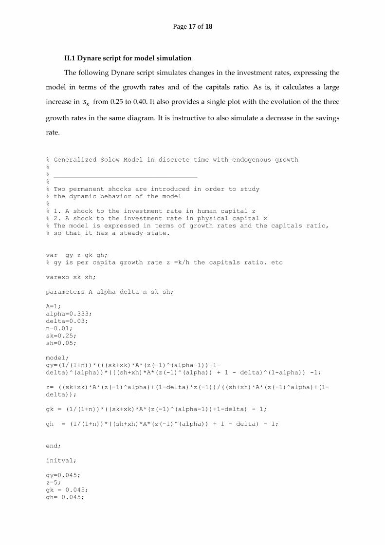
II.1 Dynare script for model simulation
The following Dynare script simulates changes in the investment rates, expressing the
model in terms of the growth rates and of the capitals ratio. As is, it calculates a large
increase in Ks from 0.25 to 0.40. It also provides a single plot with the evolution of the three
growth rates in the same diagram. It is instructive to also simulate a decrease in the savings
rate.
% Generalized Solow Model in discrete time with endogenous growth
%
% _____________________________________
%
% Two permanent shocks are introduced in order to study
% the dynamic behavior of the model
%
% 1. A shock to the investment rate in human capital z
% 2. A shock to the investment rate in physical capital x
% The model is expressed in terms of growth rates and the capitals ratio,
% so that it has a steady-state.
var gy z gk gh;
% gy is per capita growth rate z =k/h the capitals ratio. etc
varexo xk xh;
parameters A alpha delta n sk sh;
A=1;
alpha=0.333;
delta=0.03;
n=0.01;
sk=0.25;
sh=0.05;
model;
gy=(1/(1+n))*(((sk+xk)*A*(z(-1)^(alpha-1))+1-
delta)^(alpha))*(((sh+xh)*A*(z(-1)^(alpha)) + 1 - delta)^(1-alpha)) -1;
z= ((sk+xk)*A*(z(-1)^alpha)+(1-delta)*z(-1))/((sh+xh)*A*(z(-1)^alpha)+(1-
delta));
gk = (1/(1+n))*((sk+xk)*A*(z(-1)^(alpha-1))+1-delta) - 1;
gh = (1/(1+n))*((sh+xh)*A*(z(-1)^(alpha)) + 1 - delta) - 1;
end;
initval;
gy=0.045;
z=5;
gk = 0.045;
gh= 0.045;
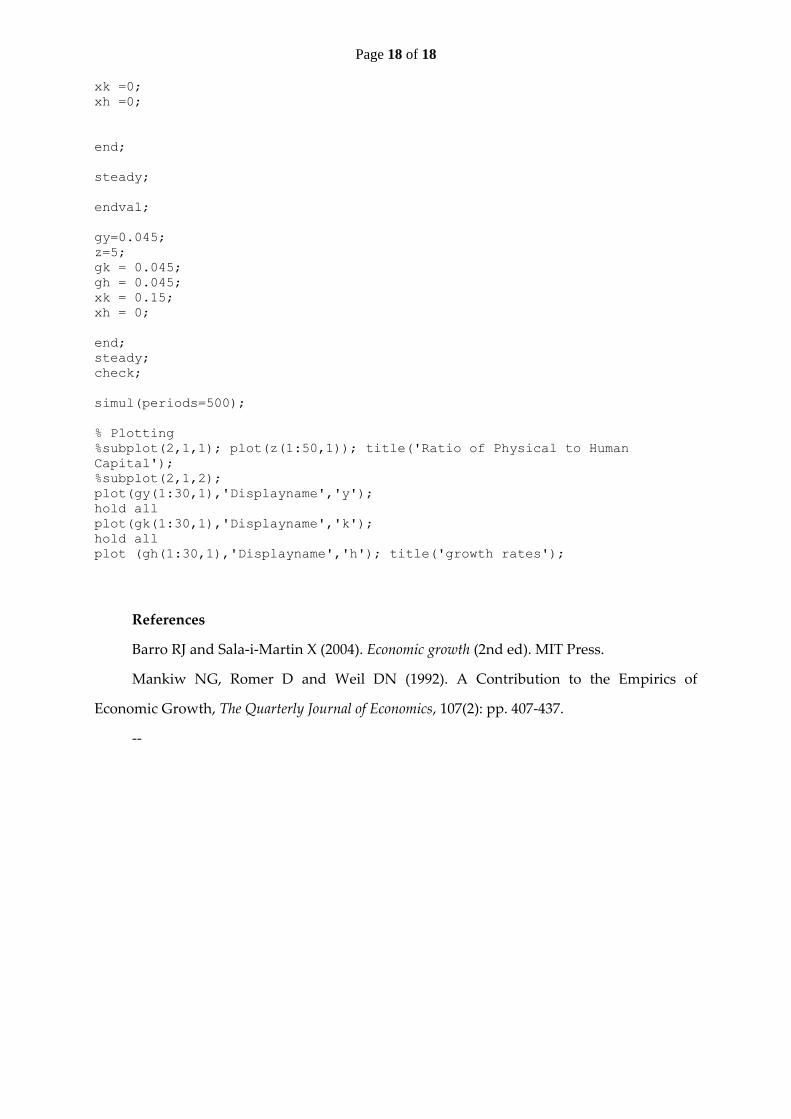
Page 18 of 18
xk =0;
xh =0;
end;
steady;
endval;
gy=0.045;
z=5;
gk = 0.045;
gh = 0.045;
xk = 0.15;
xh = 0;
end;
steady;
check;
simul(periods=500);
% Plotting
%subplot(2,1,1); plot(z(1:50,1)); title('Ratio of Physical to Human
Capital');
%subplot(2,1,2);
plot(gy(1:30,1),'Displayname','y');
hold all
plot(gk(1:30,1),'Displayname','k');
hold all
plot (gh(1:30,1),'Displayname','h'); title('growth rates');
References
Barro RJ and Sala-i-Martin X (2004). Economic growth (2nd ed). MIT Press.
Mankiw NG, Romer D and Weil DN (1992). A Contribution to the Empirics of
Economic Growth, The Quarterly Journal of Economics, 107(2): pp. 407-437.
--