Probabilistic Modelling of the Joint Labour Decisions of Husband and Wife in Farm Households

By Hild-Marte Bjørnsen

Norwegian Institute for Urban and Regional Research

Paper Presented at Workshop on the Farm Household-Firm Unit:

Its importance in agriculture and implications for statistics 12-13 April 2002

Wye Campus Imperial College, University of London

Probabilistic Modelling of the Joint Labour Decisions of

Husband and Wife in Farm Households

Hild-Marte Bjørnsen

Norwegian Institute for Urban and Regional Research

P.O.Box 44 Blindern, N-0313 Oslo, Norway

Tel: +47 22 95 89 65

Fax: +47 22 60 77 74

Email: marte.bjornsen@nibr.no

Web: www.nibr.no

Abstract When working with micro data one sometimes encounters situations involving

qualitative choices in addition to the continuous choices that are the traditional focus

of empirical analysis. One such situation arises when we study the increase in

multiple job-holdings among farm operators in western economies. In these analyses

we are both interested in the qualitative choice of entering the off-farm labour market

and the continuous choice of determining labour supply in all occupations. This paper

presents a unified framework for formulating such a discrete/continuous choices that

include randomness within the decision-making process. We consider the joint labour

decisions of operator and spouse through an agricultural household model that

combines the agricultural production, consumption, and labour supply decisions in a

single framework. We develop a probabilistic decision rule for participating in off-

farm work and derive the demand functions in farm production and labour supply

functions in off-farm sector.

1

Introduction Most articles concerning labour decisions of farm households are based on

neoclassical theory. The central assumption of the theory is that of optimisation and

the individuals/households are assumed to maximize their utility, which is a function

of consumption goods and leisure time, subject to constraints on time, income and

farm production. For an individual to be able to rank all his alternative allocations

there are certain key assumptions that must be satisfied to give the desired properties

to an individual’s preference ordering. First of all, we must assume that the individual

has unlimited information of all possible alternative allocations. Secondly, we must

assume that he is able to rank all alternatives in a consistent and well-defined order,

however alike or unlike they may be. This includes the assumption of transitivity

which states that if a is preferred to b and b is preferred to c, then a must be preferred

to c, and the assumption of reflexivity which states that all alternatives are preferred or

indifferent to itself. These assumptions allow us to partition any given allocation into

non-intersecting indifference curves that can be illustrated in a two-dimensional

diagram where consumption of consumer goods is represented along the x-axis and

consumption of leisure along the y-axis1. To give these indifference curves a

particular structure we usually add assumptions of non-satiation (alternative a is

preferred to alternative b if a contains more of at least one good and no less of any

other), continuity of the indifference curves (changes in consumption of purchased

goods can be fully compensated by changes in consumption of leisure), and strict

convexity (the set of alternatives that are preferred to alternative a is strictly convex).

The neoclassical approach can be criticized for not giving a very adequate description

of human behaviour. People don’t usually have perfect information of the alternatives

they can choose among and the choices they make are not necessarily consistent with

their previous behaviour. It is not difficult to picture a situation where we get

problems with ranking the alternatives we face. Even the simplest comparisons may

cause uncertainties; given that I am feeling a bit peckish, do I prefer a sandwich or

would I be better off by spending my last money on a pint of lager? Often we find that 1 We treat the vector of all purchased consumption goods as one argument of the utility function and the household’s leisure as a second argument. The household’s preferences can then be presented as indifference curves in a two-dimensional diagram.

2

the choice alternatives are much more complex than this example. It is also highly

probable that our preferences change over time. They may even change within a few

minutes depending on what new information or shock that occurs. I may go from

peckish to hungry within a short while and actually go for the sandwich! A

household’s preferences for leisure may be dependent on household characteristics

like number and age of children, with personal characteristics like age and education,

and with local labour market characteristics. In this case there exists exogenous

variables that affect the choices the household makes.

Some argue that choice behaviour should be modelled as a probabilistic process to

account for the individuals’ uncertainty and for the observed inconsistency (Tversky

1972). This approach implies that we associate probabilities with either of the

alternatives. If we are going to introduce probabilistic processes in our model, we

need to consider what factors determine the probabilities. Shall we focus on the

inconsistencies in the individuals’ behaviour or are the measurement problems and

inappropriate model specifications of greater concern? We must also distinguish

between models with stochastic decision rules (and deterministic utility) and models

with stochastic utility (and deterministic decision rule), respectively. In the first case

we have a situation where an individual don’t necessarily choose the alternative that

brings him the higher utility, while in the second case the individual will choose the

alternative that he expects will bring him the higher utility The second alternative is

thus closer to the neoclassical models.

We can think of several reasons why we may not be able to model the labour

decisions of the multiple-job holding households correctly. A common, and more or

less unavoidable, problem is that we can’t fully observe all the factors that enter into

the individuals’ utility functions. We may i.e. have insufficient knowledge of

preferences for farming and attachment to the farm property (maintenance of family

traditions ect). This kind of heterogeneity in preferences will lead to greater variance

in our estimates. Another source of uncertainty may stem from insufficient recordings

of observable variables like farm characteristics, household/individual characteristics,

and regional characteristics. A seemingly important explanatory variable when

estimating off-farm labour supply that more often than not seems to be absent from

the reaserchers’ data sets, is the individuals level of education. The lack of such

3

variables contributes to increase the unexplained part of the model. According to

Manski (1977) the different sources of uncertainty can be listed in four groups: Non-

observable characteristics (when the vector of characteristics affecting the choice of

the individual is only partially known by the modeler), non-observable variations in

individual utilities (when the variance in preferences increase with increasing

preference heterogeneity), measurement errors (when the amount of the observable

characteristics is not perfectly known) and functional misspecifications (when the

functional form of utility is not known with certainty).

Theoretical Model We view the decision to participate in off-farm wage work by farm operators (O) and

their spouses (S) through an agricultural household model that combines agricultural

production, consumption and labour supply decisions into a single framework. The

model bear resemblance to models used by Huffman and Lange (1989), Gould and

Saupe (1989), Lass and Gempesaw (1992), and Weersink, Nicholson and Weerhewa

(1997).

The population of farm household face the same choice set of alternative occupations.

We assume that they are statistically identical and independently distributed. This

assumption implies that their choices are governed by the same mulitnominal

distribution and that the choices made by one household are independent of the

choices made by others. The actual time allocations are allowed to vary between

households.

I was planning to choose a random utility approach to model the off-farm labour

decisions based on McFadden’s conditional logit model. My aim was to let the

households maximize utility by choosing among four alternative allocations:

D1 both operator and spouse participate in wage work: M MO S> >0 0,

D2 only operator participates in wage work: M MO S> =0 0,

D3 only spouse participates in wage work: M MO S= >0 0,

D4 neither of them participates in wage work: M MO S= =0 0,

4

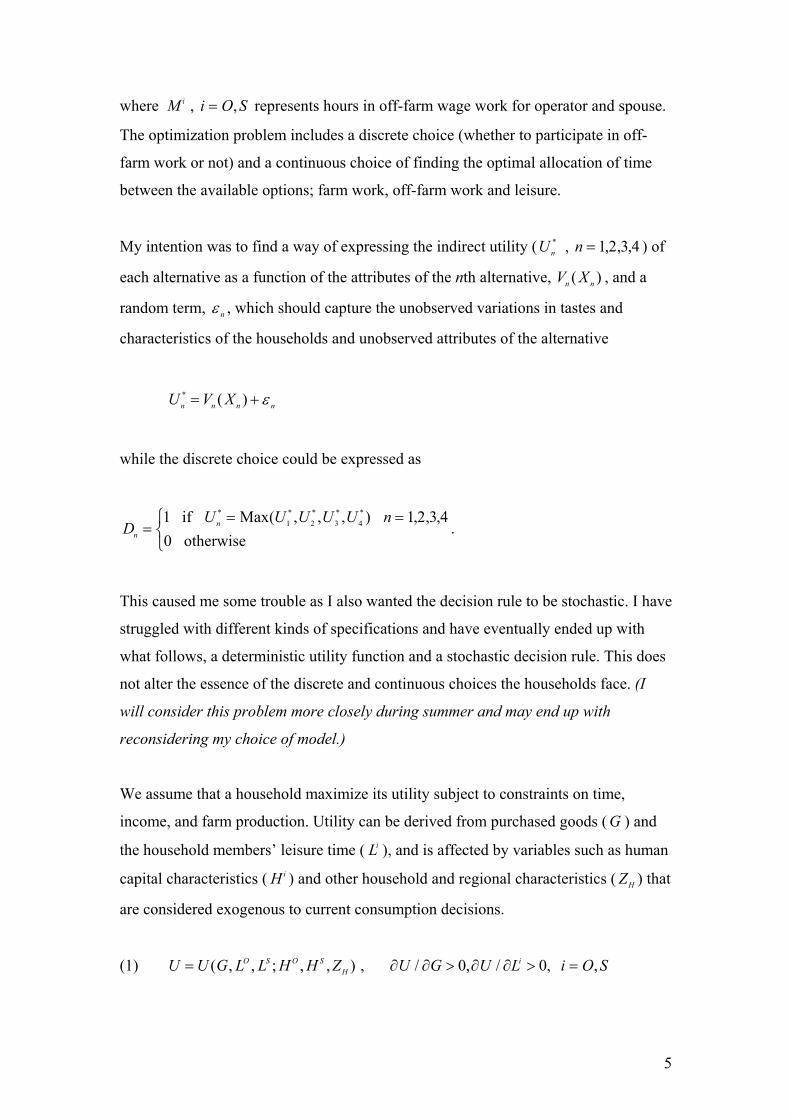
where represents hours in off-farm wage work for operator and spouse.

The optimization problem includes a discrete choice (whether to participate in off-

farm work or not) and a continuous choice of finding the optimal allocation of time

between the available options; farm work, off-farm work and leisure.

M i O Si , = ,

My intention was to find a way of expressing the indirect utility (U n ) of

each alternative as a function of the attributes of the nth alternative, V X , and a

random term,

n* , , , , = 1 2 3 4

n n( )

ε n , which should capture the unobserved variations in tastes and

characteristics of the households and unobserved attributes of the alternative

U V Xn n n* ( )= + nε

while the discrete choice could be expressed as

DU U U U U n

nn== =RST

1 10

1 2 3 4 if Max otherwise

* * * * *( , , , ) , , ,2 3 4.

This caused me some trouble as I also wanted the decision rule to be stochastic. I have

struggled with different kinds of specifications and have eventually ended up with

what follows, a deterministic utility function and a stochastic decision rule. This does

not alter the essence of the discrete and continuous choices the households face. (I

will consider this problem more closely during summer and may end up with

reconsidering my choice of model.)

We assume that a household maximize its utility subject to constraints on time,

income, and farm production. Utility can be derived from purchased goods ( G ) and

the household members’ leisure time ( ), and is affected by variables such as human

capital characteristics (

Li

Hi ) and other household and regional characteristics ( ) that

are considered exogenous to current consumption decisions.

ZH

(1) U U G L L H H Z U G U L i O SO S O SH

i= ∂ ∂ > ∂ ∂ > =( , , ; , , ) / , / , , , 0 0

5

The utility function is assumed to be ordinal and strictly concave and is maximized

subject to constraints on time, income and farm productivity. We let 24 hours be the

total time endowment ( T ) in this model and assume that time for operator and spouse

are heterogeneous. Time can be spent on leisure (home work, sleep, leisure time ect.)

denoted , farm work ( ), and wage work (Li F i M i ), all measured in number of hours.

By definition all farm households supply a positive amount of on-farm labour hours

and we assume that both operator and spouse work on the farm. We also assume that

all individuals enjoy a strictly positive number of non-working hours. Time spent in

off-farm sector is a non-negative variable for both operator and spouse.

(2) T F M L F L M i O Si i i i i i= + + > ≥ = , , , , ,0 0

The consumption of market goods at price will be limited by available income

earned from farm profits, net income from wage work, and other household income,

. The farm households are assumed to be competitive in input and output markets

and farm profit is set equal to the price of farm output ( ) multiplied with output

( Q ) less the variable cost of production (

PG

V

PQ

RX ), where R is the input price vector and

X is the quantity of purchased farm inputs. Off-farm work is paid at the wage rate

. For simplicity, we don’t include taxes in the model. The budget constraint of a

household can then be represented by the following equation.

W i

(3) P G P Q RX W M W M VG QO O S S= − + + +

In the following we will treat consumer goods ( G ) as numeraire and set equal to

one.

PG

The wage rates the operator and spouse face are assumed to depend on their

respective human capital characteristics ( Hi ) and the local labour market conditions

( ). ZM

(4) W W H Z i Oi i iM= =( , ) , , S

6

We assume flexible work schedules in off farm employment so the household

members can maximize utility by offering an optimal number of off farm work hours

and that the wage rates are independent of the hours worked.

The properties of the farm production function represent a third and final constraint

on the household’s consumption abilities. Farm output is a function of the labour

hours put down in farm production ( ) and a vector of purchased farm inputs (F i X ),

and is dependent on human capital characteristics ( Hi ) and farm specific

characteristics ( ). While off farm wages were assumed to be independent of hours

worked, marginal returns to farm labour are assumed to be diminishing. The

production function is assumed to be strictly concave.

ZF

(5) Q f F F X H H ZO S O SF= ( , , ; , , )

The discrete choice of the maximization problem is to choose the alternative

( i ) that gives the household the highest utility while the continuous choice is

to find optimal labour supply in farm and off farm sector.

= 1 2 3 4, , ,

The discrete choices of the utility maximizing problem can be expressed as four

binary choice variables

(6)

D if and otherwise

D if and otherwise

D if and otherwise

D if and otherwise

1

2

3

4

=≥ ≥RST

UVW=

≥ <RSTUVW

=< ≥RST

UVW=

< <RSTUVW

10

10

10

10

W W W W

W W W W

W W W W

W W W W

O OR S SR

O OR S SR

O OR S SR

O OR S SR

where W is individual i’s reservation wage. i=O,S. iR

7

These four alternatives are mutually exclusive. The household can only choose one of

the above alternatives at a time. We can add another constraint to the maximization

problem.

(7) D D n m n mn m = ≠ =0 1 for all , , , , ,2 3 4

Let us first assume that the utility function is deterministic, i.e. the household has full

information on all arguments that’s included in the maximization problem. We get the

optimal quantities of off-farm labour supply ( M i ), the variables in household

consumption ( and ), and the variable inputs in production ( and G Li F i X ) by

maximizing utility (1) subject to constraints on time (2), budget (3) and farm

productivity (5). The Lagrange function can be expressed like

(8) + −

£ ( , , ; , , )

( , , ; , , ) ( , )

( , )

= + − −

+

+ + −

=∑U G L L H H Z T F M L

P f F F X H H Z RX W H Z M

W H Z M V G

O S O SH i

i i i

i

QO S O S

FO O

MO

S SM

S

λ

γ

c hm

r

1

2

−

Which gives the following first order conditions for an interior solution

(9) ∂∂

= − =£G

UG γ 0

(10) ∂∂

= − =£L

Ui L ii λ 0

(11) ∂∂

= − + =£ '

FP fi i Q iλ γ 0

(12) ∂∂

= − + ≤£

MWi i

iλ γ 0

(13) ∂∂

= −£ ( )'

XP f RQ Xγ 0=

We find the optimal solution by simultaneously solving the first-order conditions. We

will have an interior solution for all choice variables with a possible exception of off-

farm work hours that may be zero for either operator, spouse, or both. Neither

8

operator nor spouse will work off the farm unless the wage rate they receive exceeds

the marginal value of farm labour evaluated at the point of optimal allocation between

farm work and leisure when no off-farm hours are supplied.

Equation (13) states that the marginal value of use of purchased input factors shall

equal the marginal cost of these factors in optimum. From equations (9) to (12) we get

that, assuming interior solution, in optimum the marginal value of farm work must

equal the marginal value of off-farm work and equal the marginal rate of substitution

between leisure and consumption, i.e. marginal value of time is equal in all

employments. Consumption goods are set as numeraire ( PG = 1).

(14) P f WUUQ i

i L

G

i' = = i=O,S

If W < the individual will not supply off-farm hours and time is divided

between farm work and leisure. If W > the individual will increase his/her off-

farm hours, thereby increasing the marginal value of farm work until the marginal

returns to both kinds of employment equal the marginal rate of substitution between

the consumption goods.

i P fQ i'

i P fQ i'

Given the assumption that the farm household acts as price taker in input and output

markets, the household model is recursive if an interior solution exists for all choice

variables. Decisions on farm labour and purchased inputs are made first, and then

consumption decisions on consumption goods and leisure.

Equations (11)-(13) are then the conditions for profit maximizing usage of farm inputs

and can be solved independently of the other equations to obtain demand functions for

farm inputs:

(15) F D W W R P H H Z Z i OiF

O SQ

O SM F

* ( , , , , , , ) ,= S=

(16) X D W W R P H H Z ZXO S

QO S

M F* ( , , , , , ,= )

9

To obtain the demand functions for leisure time we need equations (2), (3), (5), (9),

and (10) conditional on (11)-(13):

(17) L D W W H H Z Z V i OiL

O S O SM H

*,( , , , , , , , ) ,= S=π

where π = − − −P Q RX W F W FQM M S S* * * *

The off-farm labour supply functions are derived residually from the time constraint

and will contain all exogenous variables in the constrained optimisation problem.

(18) M T F L

D W W P R V H H Z Z Z i O S

i i i

MO S

QO S

H F M

* * *

, , , , , , , , , ,

= − −

= = c h

If however optimal hours of off-farm work are zero for either operator or spouse,

household decisions regarding production and consumption decisions must be made

jointly, rather than recursively. Off-farm labour supply will still be made residually,

but the unobservable wage rate for an individual not working off the farm will not be

a determinant of the hours work by the other partner. Still, the supply function for this

partner is conditional upon the participation decision by the partner without off-farm

employment.

The reservation wage for participation in off-farm work for individual i is equal to the

marginal value of his/her time when all time is allocated between farm work and

leisure ( T F Li= + i

S

). This gives us the participation rule

(19) yW W P f

W W P fi O Si

i iRQ i M

i iRQ i M

i

i

=≥ =

< =

RS|T|

==

=

1

00

0

if

if

'

'

|

|,

We assume that the off-farm labour demand equations for the operator and spouse can

be expressed as a linear function of its arguments

(20) W b H b Z v W W i OiiH

iiZ M i

i iR

M i= + + > ==

if | ,0

10

where v is some random disturbance. The wage rate is observed only when the

decision to work off the farm is made which occurs if the market wage exceeds the

reservation rate. As the reservation wage equals the marginal value of farm work

when zero off-farm work hours is supplied it will depend on non-wage and non-price

variables exogenous to the household consumption ( ), production ( ) and labour

supply ( ) decisions represented by the aggregate

i

Z

ZH ZF

M Z .

The supply of off-farm labour depends on the exogenous variables Z , the price

variables P (where P is a vector P P R VQ= ( , , ) ), and the wage rates as shown in

equation (18). As mentioned, the unobservable wage rate of an individual who is not

participating in off-farm work will not be a determinant of the spouse’s supply

function. The off-farm labour supply functions of the four alternatives can be

expressed as;

(21) MM a W a W a Z a P W W W WM a W a Z a P W W W WM

O

OOO

OOS

SZO PO

O OR S

OOO

OZO PO

O OR S

O

=

= + + + ≥ ≥

= + + ≥ <

=

RS|T|

11 1 1 1

22 2 2

4 0

if if

otherwise

,,

SR

SR

SR

R

(22) MM a W a W a Z a P W W W WM a W a Z a P W W W WM

S

SSO

OSS

SZS PS

O OR S

SSS

SZS PS

O OR S S

S

=

= + + + ≥ ≥

= + + < ≥

=

RS|T|

11 1 1 1

33 3 3

4 0

if if

otherwise

,,

By inserting for W from (20) we get the labour supply equations as functions of only

the exogenous variables,

i

H i , , PQ R , V , and , where Zk k H F M= , , . We simplify

the equations by letting all exogenous variables be represented by an aggregate Y, and

get:

(21’) M

M a Y W W W W

M a Y W W W W

M

O

O O OR

O O OR

O

=

= + ≥ ≥

= + ≥ <

=

RS|

T|1

1 11

22 2

2

4 0

υ

υ

if

if

otherwise

,

,

S SR

S SR

11

(22’) M

M a Y W W W W

M a Y W W W W

M

S

S O OR

S O OR

S

=

= + ≥ ≥

= + < ≥

=

RS|

T|1

4 44

33 3

3

4 0

υ

υ

if

if

otherwise

,

,

S SR

S SR

where υ n , n={1,2,3,4}, is a random disturbance that stems from the off-farm labour

demand equations. We assume that υ is logistically distributed with distribution

function 1+ −exp( )Y1

, zero mean and variance equal to π 2 3/ .

Each individual chooses his/her course of action on the principle that the other’s

behaviour is given. The probability of participating in off-farm work will then be

defined by four conditional distributions.

(23)

Pr |exp

Pr |exp

Pr |exp

Pr |exp

y ya Y

y ya Y

y ya Y

y ya Y

O S

O S

S O

S O

= = =+

= = =+

= = =+

= = =+

1 1 11

1 0 11

1 0 11

1 1 11

1 1

2 2

3 3

4 4

m r c hm r c hm r c hm r c h

This kind of conditional behaviour is not necessarily compatible. In order to make

these conditional distributions unambiguously define a course of action, the condition

a Y a Y a Y a Y1 1 3 3 2 2 4 4+ = + must be satisfied (Gourieroux 2000:57).

When each variable can take on only two values (0,1) the conditional probabilities can

be expressed as functions of the joint probabilities as follows:

12

Pr |Pr ,

Pr , Pr ,Pr |

Pr |Pr ,

Pr , Pr ,Pr |

Pr |Pr ,

Pr ,

y yy y

y y y yP

P Py y

y yy y

y y y yP

P Py y

y yy y

y y

O SO S

O S O SO S

O SO S

O S O SO S

S OS O

S O

= = == =

= = + = ==

+= − = =

= = == =

= = + = ==

+= − = =

= = == =

= =

1 01 0

0 0 1 01 0

1 11 1

0 1 1 11 0

1 01 0

0

10

00 10

11

01 11

m r m rm r m r m r

m r m rm r m r m r

m r m r

0

1

0 1 01 0

1 11 1

0 1 1 11 0

01

00 01

11

10 11

m r m r m r

m r m rm r m r m r

+ = ==

+= − = =

= = == =

= = + = ==

+= − = =

Pr ,Pr |

Pr |Pr ,

Pr , Pr ,Pr |

y yP

P Py y

y yy y

y y y yP

P Py y

S OS O

S OS O

S O S OS O

0

1

To prove that a Y a Y a Y a Y1 1 3 3 2 2 4 4+ = + is a necessary condition we start with the

lemma:

(*) Pr | Pr |Pr | Pr |

Pr | Pr |Pr | Pr |

y y y yy y y y

y y y yy y y y

O S S O

O S S O

O S S O

O S S O

= = = =

= = = ==

= = = =

= = = =

0 0 0 11 0 1 1

0 1 01 1 1 0

m r m rm r m r

m r mm r m

0rr

This equality can be proven by replacing the conditional probabilities with the joint

probabilities:

PP P

PP P

PP P

PP P

PP P

PP P

PP P

PP P

00

00 10

10

10 11

10

00 10

11

10 11

01

01 11

00

00 01

11

01 11

01

00 01

+ +

+ +

=+ +

+ +

We can now easily see that both the left and the right hand side of the equality equals

PP

y yy y

O S

O S00

11

0 01 1

== =

= =

Pr ,Pr ,m rm r .

By replacing the conditional probabilities in (*) with the conditional logit distribution

in (23) we obtain:

1 1 0 1 1 11 0 1 1

1 1 1 1 11 1 1 0

− = = − = =

= = = ==

− = = − = =

= = = =

Pr | Pr |Pr | Pr |

Pr | Pr |Pr | Pr |

y y y yy y y y

y y y yy y y y

O S S O

O S S O

O S S O

O S S O

m rn s m rn sm r m r

m rn s m rn sm r m r

0

(**) exp( ) exp( ) exp( ) exp( )a Y a Y a Y a Ya Y a Y a Y a Y

2 2 4 4 1 1 3 3

2 2 4 4 1 1 3 3

=

+ = +

13

Which is the compatability condition.

We can now utilize this condition to express the joint probabilities. We know that the

left hand side of (**) equals PP

00

11

which implies

P a Y a Y002 2 4 4

11= +exp( )P

and from the relations between the conditional and joint probabilities we get

Pa Y

P a Y a Ya Y

P a Y10 2 2 00

2 2 4 4

2 2 114 4

11

1= =

+=

exp( )exp( )

exp( )exp( )P

P

P

P a Y011 1

11= exp( )

while can be expressed as P11

P P P11 00 10 011= − + +( )

This gives us the following probabilities for the four alternatives the household are

faced with:

Alternative : both operator and spouse work off-farm: D1

(24) Pr ,exp( ) exp( ) exp( )

y ya Y a Y a Y

O S= = =+ + +

1 1 11 11 1 4 4 2 2m r

Alternative : only operator works off-farm: D2

(25) Pr , exp( )exp( ) exp( ) exp( )

y y a Ya Y a Y a Y

O S= = =+ + +

1 01 1

4 4

1 1 4 4 2 2m r

Alternative : only the spouse works off-farm: D3

14

(26) Pr , exp( )exp( ) exp( ) exp( )

y y a Ya Y a Y a Y

O S= = =+ + +

0 11 1

1 1

1 1 4 4 2 2m r

Alternative : neither operator nor spouse works off-farm: D4

(27) Pr , exp( )exp( ) exp( ) exp( )

y y a Y a Ya Y a Y a Y

O S= = =+

+ + +0 0

1 1

2 2 4 4

1 1 4 4 2 2m r

Estimation Let Y j , represent the J possible values of the vector of explanatory

variables in (22’) and (23’), and call a “trial of type j” a run of the experiment

performed under the conditions Y Y

Jj , = 1 2, ,...,

nnj= = , ( 1 2 3 4, , , ) . Let there be such trials

(Gourieroux 2000:20).

mj

In the bivariate case as outlined above we have observations on the pairs

y y y j J iij ijO

ijS

j= = =, ,..., ,...m r , , 1 1 m

,

which assumes the values with probabilities (as given in

(24)-(27):

k k k k1 2 1 20 1 0 1, ,l q , , = =

(24’) Pa Y a Y a Y

F a Y a Y a Yj j j jj j j

11 1 1 4 4 2 211 1 1 2 2 4 41

1 1=

+ + +=

exp( ) exp( ) exp( ), ,c h

(25’) P a Ya Y a Y a Y

F a Y a Y a Yj

j

j j jj j j

10

4 4

1 1 4 4 2 210 1 1 2 2 4 4

1 1=

+ + +=

exp( )exp( ) exp( ) exp( )

, ,c h

15

(26’) P a Ya Y a Y a Y

F a Y a Y a Yj

j

j j jj j j

01

1 1

1 1 4 4 2 201 1 1 2 2 4 4

1 1=

+ + +=

exp( )exp( ) exp( ) exp( )

, ,c h

(27’) P a Y a Ya Y a Y a Y

F a Y a Y a Yooj

j j

j j jj j j=

++ + +

=exp( )

exp( ) exp( ) exp( ), ,

2 2 4 4

1 1 4 4 2 200 1 1 2 2 4 4

1 1c h

The probability distribution functions are all strictly positive, F kk k1 2 0 1 2> ∀, , k

and constrained by

F k k

kk

1 2

21 0

1

0

1

1==∑∑ =

and the compatability constraint a Y a Y a Y a Y1 1 3 3 2 2 4 4+ = + .

The log of the likelihood function is then given by

(28) log ( ; ) log[ ( )]L y a m P ak k jkkj

J

k k j=

===∑∑∑ 1 2 1 2

21 0

1

0

1

1

The maximum likelihood estimator is obtained by writing the first-order conditions

0

01 2

1 2

1 221 0

1

0

1

1

=∂∂

====∑∑∑

log( )

( )( )

La

m F jF j

Y

n

k k jnk k

k k jn

kkj

J

where indicates the partial derivative of with respect to the n-th

coordinate.

Fnk k1 2 ( )j jF k k1 2 ( )

16

The maximum likelihood estimator α ML

)j

which solves the equation system converges

asymptotically ( ,J mj fixed, →∞ ∀ to a ,

a =

F

H

GGGG

I

K

JJJJ

aaaa

1

2

3

4

and is asymptotically normally distributed α MLasy

nN E La a

→ −∂∂ ∂LNM

OQP

RS|T|UV|W|

−

a; log( )'

2 1

l.

We find the asymptotic covariance matrix of α ML by taking the second derivatives of

the log likelihood function

∂∂ ∂

=∂

∂LNM

OQP

=−

+LNM

OQP

===

===

∑∑∑

∑∑∑

2

0

1

0

1

1

20

1

0

1

1

1 2

1 2

1 221

1 2

1 2 1 2

1 2

1 2

1 221

log( )( )' ( )'

( )( )

( ) ( )( ) ( )

( )( )

( )'

La a

ma

F jF j

Y

m F j F jF j

F jF j

Y Y

n k k jnk k

k kk

jn

kj

J

k k jnk k k k

k knk k

k kk

jn

kj

J

j

l l

l l l

According to Gourieroux (2000:93) a much simpler estimation method for the

conditional logit model is given as follows:

If we let π k k jj

mm

k k j

1 2

1 2= be the observed frequencies for each trial of type j, a we can

be estimated simply by calculating the conditional frequency

1

ππ π

11

01 11

j

j j+ and applying

the Berkson’s method. Then the observed frequencies π k k j1 2 asymptotically converges

to the true probabilities . I will not explain the Berkson method in any further

detail.

P ak k j1 2

( )

17

Data The data for my analysis can mainly be obtained from a yearly survey of Norwegian

farm households (Account Results in Agriculture and Forestry) collected by the

Norwegian Agricultural Economics Research Institute (NILF). The survey is one of

the more comprehensive sources of farm statistics in Norway, but has so far had little

widespread use in applied research. The survey dates back to the beginning of the

20th century and has since 1950 included approximately 1000 farm households

representing different regions and principal productions (grain, dairy, livestock etc.).

Participation in the survey is voluntary but restricted to farmers younger than the age

of 67 (retirement age) and to farm households working at least 400 on-farm hours on

a yearly basis. Farms that produce both grain and swine products, and dairy farms

(pure dairy farms or dairy in combination with livestock production) have the highest

representation both in absolute numbers and as share of the total population. Most

farm households in the survey report between 1800 and 6000 on-farm work hours

yearly, while a standard man-labour year in the agricultural sector is set like 1875

hours. There is no specific decision rule used for entering new households, but one

aims to enter farm households that hold more or less the same characteristics

(region/size/production) as the exiting farms. Somewhere between five and ten

percent of the farm households are replaced each year, most commonly because the

exiting households don’t wish to continue being part of the survey.

The Account Results in Agriculture and Forestry is the most elaborate source of

information on Norwegian farm households financial matters both in a regional and a

production type of context. The survey includes data on daily or weekly labour hours

for all household members, family members, and hired help and in all employments.

On-farm labour compensation is calculated using the cost of hired help, added holiday

allowances and social security payments, and off-farm income is divided between

wage work and other income. The survey also includes data on total area of cultivated

land and the division of land into different uses and the yield of and income from

different agricultural crops, fruit, garden berries and vegetables. To allow for

calculation of obtained prices from farm sales, the turnover from all farm products are

registered. Also the household’s consumption of own production is registered. All

costs of production are reported in total figures for each and every production input.

18

Finally, the survey includes detailed balance sheets information and profit and loss

accounts for all households, including information on production grants, interest

payments, tax payments, and investment grants. The data set does not contain

information on personal and family characteristics such as education, martial status,

and family size which have been found to be important explanatory variables in

estimating farmers’ off-farm work participation and off-farm labour supply (see e.g.

Huffman 1980 and Weersink 1992).

Sample selection I have not yet tried to estimate my model on the data described above. I will need to

decide on what empirical model best suits my purpose and I plan to run some

estimations during summer. I plan to extract a ten-year panel, 1991-2000, from the

Account Results survey and to account for the lacking variables of this survey by

matching the data with statistics from Statistics Norway to be able to include at least

the household members’ level of education and family size. I have not yet decided

exactly what variables will be included in the estimations.

Comments and further challenges As I mentioned at the beginning of this paper my intention was to specify a random

utility model inspired by the work of Hanemann (1984) though probably following

the outline of McFaddens conditional logit model. This proved to be a rather complex

problem and the main obstacle is that my problem is to derive labour supply equations

that does not directly enter the utility function.

My confusion was based on the selection of discrete choice variable, either:

Choose the alternative that generates the higher utility:

DU U U U U n

nn== =RST

1 10

1 2 3 4 if Max otherwise

* * * * *( , , , ) , , ,2 3 4

or

choose the participation rule:

yW W P f

W W P fi O Si

i iRQ i M

i iRQ i M

i

i

=≥ =

< =

RS|T|

==

=

1

00

0

if

if

'

'

|

|,

19

I am uncertain whether these discrete choices can be integrated within a single

framework for a two-stage estimation or not, where

Stage one: Calculate the probability of choosing alternative n

Stage two: Choose the alternative that yields the higher utility

A matter that needs further investigation is my choice of participation rule for off-

farm labour supply. I doubt the definition of the reservation wage I have used is very

adequate, particularly for the spouses. Another question is whether it is relevant for

my problem to include the joint decisions of husband and wife if the off-farm labour

decisions of the spouses are independent of the farm production decisions. I have been

considering whether the tobit model might better serve my purpose, and I also have to

extend the model framework to account for the panel structure of my data.

20

Literature

Anderson, S.P., A. De Palma, and J.-F. Thisse. (1992): Discrete Chioce Theory of

Product Differentiation. Cambridge: MIT Press.

Gould, B.W, and W.E. Saupe. (1989): “Off farm labor market entry and exit.” Amer.

J. Agr. Econ. 71, 960-967.

Gourieroux, C. (2000): Econometrics of Qualitative Dependent Variables. Cambridge

University Press.

Greene, W.H. (1997): Econometric Analysis. Prentice-Hall, New Jersey.

Hanemann, W.M. (1984): “Discrete/Continuous Models of Consumer Demand.”

Econometrica Vol. 52, Issue 3, 541-562.

Huffman, W.E., and H. El-Osta. (1998): “Off-Farm Work Participation, Off-Farm

Labor Supply and On-Farm Labor Demand of U.S. Farm Operators.”

American Journal of Agricultural Economics. 80, 1180-.

Huffman, W.E., and M.D. Lange. (1989): “Off-farm work decisions of husbands and

wives: joint decision making.” Review of Economics and Statistics. 71, 471-

480.

Lass, D.A., and C.M. Gempesaw II. (1992): “The Supply of Off-Farm Labor: A

Random Coefficient Approach.” Amer. J. Agr. Econ. 74, 400-411.

Maddala, G.S. (1983): Limited-dependent and qualitative variables in econometrics.

Cambridge University Press.

Manski, C. F. (1977): ”The Structure of Random Utility Models.” Theory and

Decision 8: 229-254.

21

Tversky, A. (1972): “Elimination by Aspects: A Theory of Choice.” Psychological

Rewiev 79: 281-299.

Weersink, A., Nicholson, C., and J. Weerhewa. (1998): “Multiple job holdings among

dairy farm families in New York and Ontario.” Agricultural Economics. 18,

127-143.

22